Physics at the $e^+ e^-$ linear collider

Abstract

A comprehensive review of physics at an $e^+e^-$ linear collider in the energy range of $\sqrt{s}=92$ GeV–3 TeV is presented in view of recent and expected LHC results, experiments from low-energy as well as astroparticle physics. The report focusses in particular on Higgs-boson, top-quark and electroweak precision physics, but also discusses several models of beyond the standard model physics such as supersymmetry, little Higgs models and extra gauge bosons. The connection to cosmology has been analysed as well.

1 Executive summary

1.1 Introduction

With the discovery of a Higgs boson with a mass of about $m_H= 125$ GeV based on data runs at the large hadron collider in its first stage at $\sqrt{s}=7$ and 8 TeV, the striking concept of explaining ‘mass’ as consequence of a spontaneously broken symmetry received a decisive push forward. The significance of this discovery was acknowledged by the award of the Nobel prize for physics to Higgs and Englert in 2013 [1–4]. The underlying idea of the Brout–Englert–Higgs (BEH) mechanism is the existence of a self-interacting Higgs field with a specific potential. The peculiar property of this Higgs field is that it is non-zero in the vacuum. In other words the Higgs field provides the vacuum with a structure. The relevance of such a field not only for our understanding of matter but also for the history of the universe is obvious.

The discovery of a Higgs boson as the materialisation of the Higgs field was the first important step in accomplishing our present level of understanding of the fundamental interactions of nature and the structure of matter that is adequately described by the standard model (SM). In the SM the constituents of matter are fermions, leptons and quarks, classified in three families with identical quantum properties. The electroweak and strong interactions are transmitted via the gauge bosons described by gauge field theories with the fundamental symmetry group $SU(3)_C\times SU(2)_L\times U(1)_Y$.

However, the next immediate steps are to answer the following questions:

• Is there just one Higgs?

• Does the Higgs field associated to the discovered particle really cause the corresponding couplings with all particles? Does it provide the right structure of the vacuum?

• Is it a SM Higgs (width, couplings, spin)? Is it a pure ${\textit{CP}}$-even Higgs boson as predicted in the SM, or is it a Higgs boson from an extended Higgs sector, possibly with some admixture of a ${\textit{CP}}$-odd component? To which model beyond the standard model (BSM) does it point?

In order to definitively establish the mechanism of electroweak symmetry breaking (EWSB), all Higgs-boson properties (mass, width, couplings, quantum numbers) have to be precisely measured and compared with the mass of the corresponding particles.

The LHC has excellent prospects for the future runs¹ 2 and 3 where proton–proton beams collide with an energy of $\sqrt{s}=13$ TeV starting in spring 2015, continued by runs with a foreseen high luminosity upgrade in the following decade [6]. High-energy $e^+e^-$-colliders have already been essential instruments in the past to search for the fundamental constituents of matter and establish their interactions. The most advanced design for a future lepton collider is the International Linear Collider (ILC) that is laid out for the energy range of $\sqrt{s}=90$ GeV–1 TeV [7, 8]. In case a drive beam accelerator technology can be applied, an energy frontier of about 3 TeV might be accessible with the Compact Linear Collider (CLIC) [9, 10].

At an $e^+e^-$ linear collider (LC) one expects rather clean experimental conditions compared to the conditions at the LHC where one has many overlapping events due to the QCD background from concurring events. A direct consequence is that one does not need any trigger at an LC but can use all data for physics analyses. Due to the collision of point-like particles the physics processes take place at the precisely and well-defined initial energy $\sqrt{s}$, both stable and measurable up to the per-mille level. The energy at the LC is tunable which offers to perform precise energy scans and to optimise the kinematic conditions for the different physics processes, respectively. In addition, the beams can be polarised: the electron beam up to about 90 %, the positron beam up to about 60 %. With such a high degree of polarisation, the initial state is precisely fixed and well known. Due to all these circumstances the final states are generally fully reconstructable so that numerous observables as masses, total cross sections but also differential energy and angular distributions are available for data analyses.

The quintessence of LC physics at the precision frontier is high luminosity and beam polarisation, tunable energy, precisely defined initial state and clear separation of events via excellent detectors. The experimental conditions that are necessary to fulfil the physics requirements have been defined in the LC scope documents [11].

Such clean experimental conditions for high-precision measurements at a LC are the ‘sine qua non’ for resolving the current puzzles and open questions. They allow one to analyse the physics data in a particularly model-independent approach. The compelling physics case for a LC has been described in numerous publications as, for instance [7, 8, 12–16], a short and compact overview is given in [17].

Although the SM has been tremendously successful and its predictions experimentally been tested with accuracies at the quantum level, i.e. significantly below the 1-per-cent level, the SM cannot be regarded as the final theory describing all aspects of nature. Astro-physical measurements [18, 19] are consistent with a universe that contains only 4 % of the total energy composed of ordinary mass but hypothesise the existence of dark matter (DM) accounting for 22 % of the total energy that is responsible for gravitational effects although no visible mass can be seen. Models accounting for DM can easily be embedded within BSM theories as, for instance, supergravity [20]. The strong belief in BSM physics is further supported by the absence of gauge coupling unification in the SM as well as its failure to explain the observed existing imbalance between baryonic and antibaryonic matter in our universe. Such facets together with the experimental data strongly support the interpretation that the SM picture is not complete but constitutes only a low-energy limit of an all-encompassing ‘theory of everything’, embedding gravity and quantum theory to describe all physical aspects of the universe. Therefore experimental hints for BSM physics are expected to manifest themselves at future colliders and model-independent strategies are crucial to determine the underlying structure of the model.

A priori there are only two approaches to reveal signals of new physics and to manifest the model of BSM at future experiments. Since the properties of the matter and gauge particles in the SM may be affected by the new energy scales, a ‘bottom-up’ approach consists in performing high precision studies of the top, Higgs and electroweak gauge bosons. Deviations from those measurements to SM predictions reveal hints to BSM physics. Under the assumption that future experiments can be performed at energies high enough to cross new thresholds, a ‘top-down’ approach becomes also feasible where the new particles or interactions can be produced and studied directly.

Obviously, the complementary search strategies at lepton and hadron colliders are predestinated for such successful dual approaches. A successful high-energy LC was already realised in the 1990s with the construction and running of the SLAC Linear Collider (SLC) that delivered up to $5\times 10^{10}$ particles per pulse. Applying in addition highly polarised electrons enabled the SLC to provide the best single measurement of the electroweak mixing angle with $\delta \sin ^2\theta _W \sim 0.00027$.

However, such a high precision manifests a still-existing inconsistency, namely the well-known discrepancy between the left–right polarisation asymmetry at the Z-pole measured at SLC and the forward–backward asymmetry measured at LEP [21]. Both values lead to measured values of the electroweak mixing angle $\sin ^2\theta _\mathrm{eff}$ that differ by more than 3$\sigma$ and point to different predictions for the Higgs mass, see Sect. 4 for more details. Clarifying the central value as well as improving the precision is essential for testing the consistence of the SM as well as BSM models.

Another example for the relevance of highest precision measurements and their interplay with most accurate theoretical predictions at the quantum level is impressively demonstrated in the interpretation of the muon anomalous moment $g_{\mu }-2$ [22]. The foreseen run of the $g_{\mu }-2$ experiment at Fermilab, starting in 2017 [23, 24], will further improve the current experimental precision by about a factor of 4 and will set substantial bounds to many new physics models via their high sensitivity to virtual effects of new particles.

The LC concept has been proposed already in 1965 [25] for providing electron beams with high enough quality for collision experiments. In [26] this concept has been proposed for collision experiments at high energies in order to avoid the energy loss via synchrotron radiation: this energy loss per turn scales with $E^4/r$, where E denotes the beam energy and r the bending radius. The challenging problems at the LC compared to circular colliders, however, are the luminosity and the energy transfer to the beams. The luminosity is given by

$$\begin{aligned} {\mathscr {L}}\sim \frac{\eta P N_e}{\sigma _{xy} E_{\mathrm{c.m.}}}, \end{aligned}$$

(1)

where P denotes the required power with efficiency $\eta$, $N_e$ the charge per bunch, $E_{\mathrm{c.m.}}$ the centre-of-mass energy and $\sigma _{xy}$ the transverse geometry of the beam size. From Eq. (1), it is obvious that flat beams and a high bunch charge allow high luminosity with lower required beam power $P_b=\epsilon P$. The current designs for a high-luminosity $e^+e^-$ collider, ILC or CLIC, is perfectly aligned with such arguments. One expects an efficiency factor of about $\eta \sim 20\,\%$ for the discussed designs.

The detectors are designed to improve the momentum resolution from tracking by a factor 10 and the jet-energy resolution by a factor 3 (in comparison with the CMS detector) and excellent $\tau ^{\pm }$-, b-, $\bar{b}$- and c, $\bar{c}$-tagging capabilities [8], are expected.

As mentioned before, another novelty is the availability of the polarisation of both beams, which can precisely project out the interaction vertices and can analyse its chirality directly.

The experimental conditions to achieve such an unprecedented precision frontier at high energy are high luminosity (even about three orders of magnitude more particles per pulse, $5\times 10^{13}$ than at the SLC), polarised electron/positron beams, tunable energy, luminosity and beam-energy stability below $0.1\,\%$ level [11]. Assuming a finite total overall running time it is a critical issue to divide up the available time between the different energies, polarisations and running options in order to maximise the physical results. Several running scenarios are thoroughly studied [27].

In the remainder of this chapter we summarise the physics highlights of this report. The corresponding details can be found in the following chapters. Starting with the three safe pillars of LC physics – Higgs-, top- and electroweak high precision physics – Sect. 2 provides a comprehensive overview about the physics of EWSB. Recent developments in LHC analyses as well as on the theory side are included, alternatives to the Higgs models are discussed. Section 3 covers QCD and in particular top-quark physics. The LC will also set a new frontier in experimental precision physics and has a striking potential for discoveries in indirect searches. In Sect. 4 the impact of electroweak precision observables (EWPO) and their interpretation within BSM physics are discussed. Supersymmetry (SUSY) is a well-defined example for physics beyond the SM with high predictive power. Therefore in Sect. 5 the potential of a LC for unravelling and determining the underlying structure in different SUSY models is discussed. Since many aspects of new physics have strong impact on astroparticle physics and cosmology, Sect. 6 provides an overview in this regard.

The above-mentioned safe physics topics can be realised at best at different energy stages at the linear collider. The possible staged energy approach for a LC is therefore ideally suited to address all the different physics topics. For some specific physics questions very high luminosity is required and in this context also a high-luminosity option at the LC is discussed, see [27] for technical details. The expected physics results of the high-luminosity LC was studied in different working group reports [28, 29], cf. Sect. 2.3.

Such an optimisation of the different running options of a LC depends on the still awaited physics demands. The possible physics outcome of different running scenarios at the LC are currently under study [27], but fixing the final running strategy is not yet advisable.

One should note, however, that such a large machine flexibility is one of the striking features of a LC.

1.2 Physics highlights

Many of the examples shown in this review are based on results of [8–10, 30, 31] and references therein.

1.2.1 Higgs physics

The need for precision studies of the new boson, compatible with a SM-like Higgs, illuminates already the clear path for taking data at different energy stages at the LC.

For a Higgs boson with a mass of 125 GeV, the first envisaged energy stage is at about $\sqrt{s}=250$ GeV: the dominant Higgs-strahlung process peaks at $\sqrt{s}=240$ GeV. This energy stage allows the model-independent measurement of the cross section $\sigma (HZ)$ with an accuracy of about 2.6 %, cf. Sect. 2.3. This quantity is the crucial ingredient for all further Higgs analyses, in particular for deriving the total width via measuring the ratio of the partial width and the corresponding branching ratio. Already at this stage many couplings can be determined with high accuracy in a model-independent way: a striking example is the precision of 1.3 % that can be expected for the coupling $g_{HZZ}$, see Sect. 2.3 for more details.

The precise determination of the mass is of interest in its own right. However, it has also high impact for probing the Higgs physics, since $m_H$ is a crucial input parameter. For instance, the branching ratios $H\rightarrow ZZ^*$, $WW^*$ are very sensitive to $m_H$: a change in $m_H$ by 200 MeV shifts $\mathrm{BR}(H\rightarrow ZZ^*$ by 2.5 %. Performing accurate threshold scans enables the most precise mass measurements of $\delta m_H=40$ MeV. Furthermore and – of more fundamental relevance – such threshold scans in combination with measuring different angular distributions allow a model-independent and unique determination of the spin.

Another crucial quantity in the Higgs sector is the total width ${\varGamma }_H$ of the Higgs boson. The prediction in the SM is ${\varGamma }_H=4.07$ MeV for $m_H=125$ GeV [32]. The direct measurement of such a small width is neither possible at the LHC nor at the LC since it is much smaller than any detector resolution. Nevertheless, at the LC a model-independent determination of ${\varGamma }_H$ can be achieved using the absolute measurement of Higgs branching ratios together with measurements of the corresponding partial widths. An essential input quantity in this context is again the precisely measured total cross section of the Higgs-strahlung process. At $\sqrt{s}=500$ GeV, one can derive the total width ${\varGamma }_H$ with a precision of 5 % based on a combination of the $H\rightarrow ZZ^*$ and $WW^*$ channels. Besides this model-independent determination, which is unique to the LC, constraints on the total width can also be obtained at the LC from a combination of on- and off-shell Higgs contributions [33] in a similar way as at the LHC [34]. The latter method, however, relies on certain theoretical assumptions, and also in terms of the achievable accuracy it is not competitive with the model-independent measurement based on the production cross section $\sigma (ZH)$ [33].

At higher energy such off-shell decays of the Higgs boson to pairs of W and Z bosons offer access to the kinematic dependence of higher-dimensional operators involving the Higgs boson. This dependence allows for example the test of unitarity in BSM models [35, 36].

In order to really establish the mechanism of EWSB it is not only important to measure all couplings but also to measure the Higgs potential:

$$\begin{aligned} V=\frac{1}{2} m_H^2 \Phi ^2_H + \lambda v \Phi _H^3+\frac{1}{4} \kappa \Phi _H^4, \end{aligned}$$

where $v=246$ GeV. It is essential to measure the tri-linear coupling rather accurate in order to test whether the observed Higgs boson originates from a field that is in concordance with the observed particle masses and the predicted EWSB mechanism.² Since the cross section for double Higgs-strahlung is small but has a maximum of about 0.2 fb at $\sqrt{s}=500$ GeV for $m_H=125$ GeV, this energy stage is required to enable a first measurement of this coupling. The uncertainty scales with ${\varDelta } \lambda {/}\lambda =1.8 {\varDelta } \sigma {/}\sigma$. New involved analyses methods in full simulations aim at a precision of 20 % at $\sqrt{s}= 500$ GeV. Better accuracy one could get applying the full LC programme and going also to higher energy, $\sqrt{s}=1$ TeV.

Another very crucial quantity is accessible at $\sqrt{s}=500$ GeV: the $t\bar{t}H$-coupling. Measuring the top-Yukawa coupling is a challenging endeavour since it is overwhelmed from $t\bar{t}$-background. At the LHC one expects an accuracy of 25 % on basis of 300 fb$^{-1}$ and under optimal assumptions and neglecting the error from theory uncertainties. At the LC already at the energy stage of $\sqrt{s}=500$ GeV, it is expected to achieve an accuracy of ${\varDelta } g_{ttH}/g_{ttH}\sim 10$ %, see Sect. 2. This energy stage is close to the threshold of ttH production, therefore the cross section for this process should be small. But thanks to QCD-induced threshold effects the cross section gets enhanced and such an accuracy should be achievable with 1 ab$^{-1}$ at the LC. It is of great importance to measure this Yukawa coupling with high precision in order to test the Higgs mechanism and verify the measured top mass $m_t=y_{ttH} v/\sqrt{2}$. The precise determination of the top Yukawa coupling opens a sensitive window to new physics and admixtures of non-SM contributions. For instance, in the general two-Higgs-doublet model the deviations with respect to the SM value of this coupling can typically be as large as $\sim 20\,\%$.

Since for a fixed $m_H$ all Higgs couplings are specified in the SM, it is not possible to perform a fit within this model. In order to test the compatibility of the SM Higgs predictions with the experimental data, the LHC Higgs Cross Section Group proposed ‘coupling scale factors’ [37, 38]. These scale factors $\kappa _i$ ($\kappa _i=1$ corresponds to the SM) dress the predicted Higgs cross section and partial widths. Applying such a $\kappa$-framework, the following assumptions have been made: there is only one 125 GeV state responsible for the signal with a coupling structure identical to the SM Higgs, i.e. a pure ${\textit{CP}}$-even state, and the zero width approximation can be applied. Usually, in addition the theory assumption $\kappa _{W,Z}<1$ (corresponds to an assumption on the total width) has to be made. Using, however, LC data and exploiting the precise measurement of $\sigma (HZ)$, this theory assumption can be dropped and all couplings can be obtained with an unprecedented precision of at least 1–2 %, see Fig. 1 [39] and Sect. 2 for further details.

Fig. 1

The achievable precision in the different Higgs couplings at the LHC on bases of $3 ab^{-1}$ and 50 % improvement in the theoretical uncertainties in comparison with the different energy stages at the ILC. In the final LC stage all couplings can be obtained in the 1–2 % range, some even better [39]

Another important property of the Higgs boson that has to be determined is the ${\textit{CP}}$ quantum number. In the SM the Higgs should be a pure ${\textit{CP}}$-even state. In BSM models, however, the observed boson state a priori can be any admixture of ${\textit{CP}}$-even and ${\textit{CP}}$-odd states, it is of high interest to determine limits on this admixture. The HVV couplings project out only the ${\textit{CP}}$-even components, therefore the degree of ${\textit{CP}}$ admixture cannot be tackled via analysing these couplings. The measurements of ${\textit{CP}}$-odd observables are mandatory to reveal the Higgs ${\textit{CP}}$-properties: for instance, the decays of the Higgs boson into $\tau$ leptons provides the possibility to construct unique ${\textit{CP}}$-odd observables via the polarisation vector of the $\tau$s, see further details in Sect. 2.

1.2.2 Top-quark physics

Top-quark physics is another rich field of phenomenology. It opens at $\sqrt{s}=350$ GeV. The mass of the top quark itself has high impact on the physics analysis. In BSM physics $m_t$ is often the crucial parameter in loop corrections to the Higgs mass. In each model where the Higgs-boson mass is not a free parameter but predicted in terms of the other model parameters, the top-quark mass enters the respective loop diagrams to the fourth power, see Sect. 4 for details. Therefore the interpretation of consistency tests of the EWPO $m_W$, $m_Z$, $\sin ^2\theta _\mathrm{eff}$ and $m_H$ require the most precise knowledge on the top-quark mass. The top quark is not an asymptotic state and $m_t$ depends on the renormalisation scheme. Therefore a clear definition of the used top quark mass is needed. Measuring the mass via a threshold scan allows to relate the measured mass uniquely to the well-defined $m_t^{\overline{\mathrm{MS}}}$ mass, see Fig. 2. Therefore, this procedure is advantageous compared to measurements via continuum observables. It is expected to achieve an unprecedented accuracy of ${\varDelta } m_{t}^{\overline{\mathrm{MS}}}=100$ MeV via threshold scans. This uncertainty contains already theoretical as well as experimental uncertainties. Only such a high accuracy enables sensitivity to loop corrections for EWPO. Furthermore the accurate determination is also decisive for tests of the vacuum stability within the SM.

Fig. 2

Simulated measurement of the background-subtracted $t\bar{t}$ cross section with 10 fb$^{-1}$ per data point, assuming a top-quark mass of 174 GeV in the 1S scheme with the ILC luminosity spectrum for the CLIC-ILD detector [40]

A sensitive window to BSM physics is opened by the analysis of the top quark couplings. Therefore a precise determination of all SM top-quark couplings together with the search for anomalous couplings is crucial and can be performed very accurately at $\sqrt{s}=500$ GeV. Using the form-factor decomposition of the electroweak top quark couplings, it has been shown that one can improve the accuracy for the determination of the couplings [41] by about one order of magitude at the LC compared to studies at the LHC, see Fig. 3 and Sect. 3.

Fig. 3

Statistical precision on ${\textit{CP}}$-conserving form factors expected at the LHC [42] and at the ILC [41]. The LHC results assume an integrated luminosity of ${\mathscr {L}}=300$ fb$^{-1}$. The results for the ILC are based on an integrated luminosity of ${\mathscr {L}}=500$ fb$^{-1}$ at $\sqrt{s}=500$ GeV and a beam polarisation of $P_{e^-}=\pm 80\,\%$, $P_{e^+}=\mp 30\,\%$ [41]

1.2.3 Beyond standard model physics – “top-down”

Supersymmetry The SUSY concept is one of the most popular extensions of the SM since it can close several open questions of the SM: achieving gauge unification, providing DM candidates, stabilising the Higgs mass, embedding new sources for ${\textit{CP}}$-violation and also potentially neutrino mixing. However, the symmetry has to be broken and the mechanism for symmetry breaking is completely unknown. Therefore the most general parametrisation allows around 100 new parameters. In order to enable phenomenological interpretations, for instance, at the LHC, strong restrictive assumptions on the SUSY mass spectrum are set. However, as long as it is not possible to describe the SUSY breaking mechanism within a full theory, data interpretations based on these assumptions should be regarded as a pragmatic approach. Therefore the rather high limits obtained at the LHC for some coloured particles exclude neither the concept of SUSY as such, nor do they exclude light electroweak particles, nor relatively light scalar quarks of the third generation.

Already the energy stage at $\sqrt{s}=350$ GeV provides a representative open window for the direct production of light SUSY particles, for instance, light higgsino-like scenarios, leading to signatures with only soft photons. The resolution of such signatures will be extremely challenging at the LHC but is feasible at the LC via the ISR method, as discussed in Sect. 5.

Another striking feature of the LC physics potential is the capability to test predicted properties of new physics candidates. For instance, in SUSY models one essential paradigm is that the coupling structure of the SUSY particle is identical to its SM partner particle. That means, for instance, that the SU(3), SU(2) and U(1) gauge couplings $g_S$, g and $g^{\prime }$ have to be identical to the corresponding SUSY Yukawa couplings $g_{\tilde{g}}$, $g_{\tilde{W}}$ and $g_{\tilde{B}}$. These tests are of fundamental importance to establish the theory. Testing, in particular, the SUSY electroweak Yukawa coupling is a unique feature of LC physics. Under the assumption that the SU(2) and U(1) parameters have been determined in the gaugino/higgsino sector (see Sect. 5.7), the identity of the Yukawa and the gauge couplings via measuring polarised cross sections can be successfully performed: depending on the electron (and positron) beam polarisation and on the luminosity, a per-cent-level precision can be achieved; see Fig. 4.

Fig. 4

Equivalence of the SUSY electroweak Yukawa couplings $g_{\tilde{W}}$, $g_{\tilde{B}}$ with the SU(2), U(1) gauge couplings g, $g^{\prime }$. Shown are the contours of the polarised cross sections $\sigma _L(e^+e^-\rightarrow \tilde{\chi }^0_1\tilde{\chi }^0_2)$ and $\sigma _R(e^+e^-\rightarrow \tilde{\chi }^0_1\tilde{\chi }^0_2)$ in the plane of the SUSY electroweak Yukawa couplings normalised to the gauge couplings, $Y_L=g_{\tilde{W}}/g$, $Y_R=g_{\tilde{B}}/g^{\prime }$ [43, 44] for a scenario with the electroweak spectrum similar to the reference point SPS1a

Another important and unique feature of the LC potential is to test experimentally the quantum numbers of new physics candidates. For instance, a particularly challenging measurement is the determination of the chiral quantum numbers of the SUSY partners of the fermions. These partners are predicted to be scalar particles and to carry the chiral quantum numbers of their standard model partners. In $e^+e^-$ collisions, the associated production reactions $e^+e^-\rightarrow \tilde{e}_L^+\tilde{e}_R^-$, $\tilde{e}_R^+\tilde{e}_L^-$ occur only via t-channel exchange, where the $e^\pm$ are directly coupled to their SUSY partners $\tilde{e}^{\pm }$. Separating the associated pairs, the chiral quantum numbers can be tested via the polarisation of $e^\pm$ since chirality corresponds to helicity in the high-energy limit. As can be seen in Fig. 5, the polarisation of both beams is absolutely essential to separate the pair $\tilde{e}_L\tilde{e}_R$ [45] and to test the associated quantum numbers.

Fig. 5

Polarised cross sections versus $P_{e^-}$ (bottom panel) and $P_{e^+}$ (top panel) for $e^+e^-\rightarrow \tilde{e}\tilde{e}$-production with direct decays in $\tilde{\chi }^0_1 e$ in a scenario where the non-coloured spectrum is similar to a SPS1a-modified scenario but with $m_{\tilde{e}_L}=200$ GeV, $m_{\tilde{e}_R}=195$ GeV. The associated chiral quantum numbers of the scalar SUSY partners $\tilde{e}_{L,R}$ can be tested via polarised $e^{\pm }$-beams

Dark matter physics Weakly interacting massive particles (WIMPs) are the favourite candidates as components of the cold DM. Neutral particles that interact only weakly provide roughly the correct relic density in a natural way. Since there are no candidates for DM in the SM, the strong observational evidence for DM clearly points to physics beyond the SM. Due to precise results from cosmological observations, for instance [46, 47], bounds on the respective cross section and the mass of the DM candidates can be set in the different models. Therefore, in many models only rather light candidates are predicted, i.e. with a mass around the scale of EWSB or even lighter. That means, for instance for SUSY models with R-parity conservation, that the lightest SUSY particle, should be within the kinematical reach of the ILC. The lowest threshold for such processes is pair production of the WIMP particle. Since such a final state, however, escapes detection, the process is only visible if accompanied by radiative photons at the LC that recoil against the WIMPs, for instance, the process $e^+e^-\rightarrow \gamma \chi \chi$ [48], where $\chi$ denotes the WIMP particle in general with a spin $S_{\chi }=0,\frac{1}{2},1$. Such a process can be realised in SUSY models, in universal extra dimensions, little Higgs theories etc. The dominant SM background is radiative neutrino production, which can, efficiently be suppressed via the use of beam polarisation.

The present DM density depends strongly on the cross section for WIMP annihilation into SM particles (assuming that there exist only one single WIMP particle $\chi$ and ignoring coannihilation processes between the WIMP and other exotic particles) in the limit when the colliding $\chi$s are non-relativistic [48], depending on s- or p-wave contributions and on the WIMP mass. Due to the excellent resolution at the LC the WIMP mass can be determined with relative accuracy of the order of 1 %, see Fig. 6.

Fig. 6

WIMP mass as a function of the mass for p-wave ($J_0=1$) annihilation and under the assumption that WIMP couplings are helicity- and parity-conserving in the process $e^+e^-\rightarrow \gamma \chi \chi$ [48]. With an integrated luminosity of ${\mathscr {L}}=500$ fb$^{-1}$ and polarised beams with $P_{e^-}=+80\,\%$, $P_{e^+}=-60\,\%$ with ${\varDelta } P/P=0.25\,\%$ the reconstructed WIMP mass can be determined with a relative accuracy of the order of 1 % [49]. The blue area shows the systematic uncertainty and the red bands the additional statistical contribution. The dominant sources of systematic uncertainties are ${\varDelta } P/P$ and the shape of the beam-energy spectrum

Following another approach and parametrising DM interactions in the form of effective operators, a non-relativistic approximation is not required and the derived bounds can be compared with experimental bounds from direct detection. Assuming that the DM particles only interact with SM fields via heavy mediators that are kinematically not accessible at the ILC, it was shown in [50, 51] that the ILC could nevertheless probe effective WIMP couplings $G^\mathrm{ILC}_{\max }=g_ig_j/M^2 = 10^{-7}$ GeV$^{-2}$ (vector or scalar mediator case), or $G^\mathrm{ILC}_{\max }=g_ig_j/M = 10^{-4}$ GeV$^{-1}$ (fermionic mediator case). The direct detection searches give much stronger bounds on spin-independent (‘vector’) than on spin-dependent (‘axial-vector’) interactions under the simplifying assumption that all SM particles couple with the same strength to the DM candidate (‘universal coupling’). If the WIMP particle is rather light ($<$10 GeV) the ILC offers a unique opportunity to search for DM candidates beyond any other experiment, even for spin-independent interactions, cf. Fig. 7 (upper panel). In view of spin-dependent interactions the ILC searches are also superior for heavy WIMP particles, see Fig. 7 (lower panel).

Fig. 7

Combined limits for fermionic dark matter models. The process $e^+e^-\rightarrow \chi \chi \gamma$ is assumed to be detected only by the hard photon. The analysis has been modelled correspondingly to [49] and is based on ${\mathscr {L}}=500$ fb$^{-1}$ at $\sqrt{s}=500$ GeV and $\sqrt{s}=1$ TeV and different polarisations [50, 51]

Neutrino mixing angle Another interesting question is how to explain the observed neutrino mixing and mass patterns in a more complete theory. SUSY with broken R-parity allows one to embed and to predict such an hierarchical pattern. The mixing between neutralinos and neutrinos puts strong relations between the LSP branching ratios and neutrino mixing angles. For instance, the solar neutrino mixing angle $\sin ^2\theta _{23}$ is accessible via measuring the ratio of the branching fractions for $\tilde{\chi }^0_1 \rightarrow W^\pm \mu ^\mp$ and $W^\pm \tau ^\mp$. Performing an experimental analysis at $\sqrt{s}=500$ GeV allows one to determine the neutrino mixing angle $\sin ^2 \theta _{23}$ up to a per-cent-level precision, as illustrated in Fig. 8 [52].

Fig. 8

Achievable precision on $\sin ^2\theta _{23}$ from bi-linear R-parity-violating decays of the $\tilde{\chi }^0_1$ as a function of the produced number of neutralino pairs compared to the current precision from neutrino oscillation measurements [52]

This direct relation between neutrino physics and high-energy physics is striking. It allows one to directly test whether the measured neutrino mixing angles can be embedded within a theoretical model of high predictive power, namely a bi-linear R-parity violation model in SUSY, based on precise measurements of neutralino branching ratios [53, 54] at a future $e^+e^-$ linear collider.

1.2.4 Beyond standard model physics – “bottom-up”

Electroweak precision observables Another compelling physics case for the LC can be made for the measurement of EWPO at $\sqrt{s}\approx 92$ GeV (Z-pole) and $\sqrt{s}\approx 160$ GeV (WW threshold), where a new level of precision can be reached. Detecting with highest precision any deviations from the SM predictions provides traces of new physics which could lead to groundbreaking discoveries. Therefore, particularly in case no further discovery is made from the LHC data, it will be beneficial to perform such high-precision measurements at these low energies. Many new physics models, including those of extra large dimensions, of extra gauge bosons, of new leptons, of SUSY, etc., can lead to measurable contributions to the electroweak mixing angle even if the scale of the respective new physics particles are in the multi-TeV range, i.e. out of range of the high-luminosity LHC. Therefore the potential of the LC to measure this quantity with an unprecedented precision, i.e. of about one order of magnitude better than at LEP/SLC offers to enter a new precision frontier. With such a high precision – mandatory are high luminosity and both beams to be polarised – one gets sensitivity to even virtual effects from BSM where the particles are beyond the kinematical reach of the $\sqrt{s}=500$ GeV LC and the LHC. In Fig. 9 the prediction for $\sin ^2\theta _\mathrm{eff}$ as a function of the lighter chargino mass $m_{\tilde{\chi }^{+}_1}$ is shown. The MSSM prediction is compared with the prediction in the SM assuming the experimental resolution expected at GigaZ. In this scenario no coloured SUSY particles would be observed at the LHC but the LC could resolve indirect effects of SUSY up to $m_{\tilde{\chi }^{+}_1}\le 500$ GeV via the measurement of $\sin ^2\theta _\mathrm{eff}$ with unprecedented precision at the low energy option GigaZ, see Sect. 4 for details. The possibility to run with high luminosity and both beam polarised on these low energies is essential in these regards.

Fig. 9

Theoretical prediction for $\sin ^2\theta _\mathrm{eff}$ in the SM and the MSSM (including prospective parametric theoretical uncertainties) compared to the experimental precision at the LC with GigaZ option. A SUSY inspired scenario SPS 1a’ has been used, where the coloured SUSY particles masses are fixed to 6 times their SPS 1a’ values. The other mass parameters are varied with a common scale factor

Extra gauge bosons One should stress that not only SUSY theories can be tested via indirect searches, but also other models, for instance, models with large extra dimensions or models with extra $Z'$, see Fig. 10, where the mass of the $Z'$ boson is far beyond the direct kinematical reach of the LHC and the LC and therefore is assumed to be unknown. Because of the clean LC environment, one even can determine the vector and axial-vector coupling of such a $Z'$ model.

Fig. 10

New gauge bosons in the $\mu ^+\mu ^-$ channel. The plot shows the expected resolution at CLIC with $\sqrt{s}=3$ TeV and ${\mathscr {L}}=1$ ab$^{-1}$ on the ‘normalised’ vector $v_f^n=v'_f\sqrt{s/(m_Z'^2-s)}$ and axial-vector $a_f^n=a'_f\sqrt{s/(m_Z'^2-s)}$ couplings to a 10 TeV $Z'$ in terms of the SM couplings $v'_f$, $a'_f$. The mass of $Z'$ is assumed to be unknown, nevertheless the couplings can be determined up to a two-fold ambiguity. The colours denote different $Z'$ models [9, 10]

1.2.5 Synopsis

The full Higgs and top-quark physics programme as well as the promising programme on DM and BSM physics should be accomplished with the higher energy LC set-up at 1 TeV. Model-independent parameter determination is essential for the crucial identification of the underlying model. Accessing a large part of the particle spectrum of a new physics model would nail down the structure of the underlying physics. But measuring already only the light part of the spectrum with high precision and model-independently can provide substantial information. Table 1 gives an overview of the different physics topics and the required energy stages. The possibility of a tunable energy in combination with polarised beams, is particularly beneficial to successfully accomplish the comprehensive physics programme at high-energy physics collider and to fully exploit the complete physics potential of the future Linear Collider.

Table 1 Physics topics where the $e^+e^-$-linear collider provides substantial results at the different energy stages that are complementary to the LHC. The examples are described in the following chapters as well as in [7–10, 12–17, 27, 28, 30, 31, 55, 56]

2 Higgs and electroweak symmetry breaking

Editors: K. Fujii, S. Heinemeyer, P.M. Zerwas⁴

Contributing authors: M. Asano, K. Desch, U. Ellwanger, C. Englert, I. Ginzburg, C. Grojean, S. Kanemura, M. Krawczyk, J. Kroseberg, S. Matsumoto, M.M. Mühlleitner, M. Stanitzki.

After a brief description of the physical basis of the Higgs mechanism, we summarise the crucial results for Higgs properties in the standard model as expected from measurements at LHC and ILC/CLIC, based on the respective reports. Extensions of the SM Higgs sector are sketched thereafter, discussed thoroughly in the detailed reports which follow: portal models requiring analyses of invisible Higgs decays, supersymmetry scenarios as generic representatives of weakly coupled Higgs sectors, and finally strong interaction elements as suggested by Little Higgs models and composite models motivated by extended space dimensions.

2.1 Résumé⁵

The Brout–Englert–Higgs mechanism [1–4, 57] is a central element of particle physics. Masses are introduced consistently in gauge theories for vector bosons, leptons and quarks, and the Higgs boson itself, by transformation of the interaction energy between the initially massless fields and the vacuum expectation value of the Higgs-field. The non-zero value of the Higgs field in the vacuum, at the minimum of the potential breaking the electroweak symmetry, is generated by self-interactions of the Higgs field. The framework of the SM [58–60] demands the physical Higgs boson as a new scalar degree of freedom, supplementing the spectrum of vectorial gauge bosons and spinorial matter particles.

This concept of mass generation has also been applied, mutatis mutandis, to extended theories into which the SM may be embedded. The new theory may remain weakly interacting up to the grand-unification scale, or even the Planck scale, as familiar in particular from supersymmetric theories, or novel strong interactions may become effective already close to the TeV regime. In such theories the Higgs sector is enlarged compared with the SM. A spectrum of several Higgs particles is generally predicted, the lightest particle often with properties close to the SM Higgs boson, and others with masses typically in the TeV regime.

A breakthrough on the path to establishing the Higgs mechanism experimentally has been achieved by observing at LHC [61, 62] a new particle with a mass of about 125 GeV and couplings to electroweak gauge bosons and matter particles compatible, cum grano salis, with expectations for the Higgs boson in the (SM) [63–66].

2.1.1 Zeroing in on the Higgs particle of the SM

Within the SM the Higgs mechanism is realised by introducing a scalar weak-isospin doublet. Three Goldstone degrees of freedom are absorbed for generating the longitudinal components of the massive electroweak $W^\pm ,Z$ bosons, and one degree of freedom is realised as a scalar physical particle unitarising the theory properly. After the candidate particle has been found, three steps are necessary to establish the relation with the Higgs mechanism:

• The mass, the lifetime (width) and the spin/${\textit{CP}}$ quantum numbers must be measured as general characteristics of the particle;

• The couplings of the Higgs particle to electroweak gauge bosons and to leptons/quarks must be proven to rise (linearly) with their masses;

• The self-coupling of the Higgs particle, responsible for the potential which generates the non-zero vacuum value of the Higgs field, must be established.

When the mass of the Higgs particle is fixed, all its properties are pre-determined. The spin/${\textit{CP}}$ assignement $J^{{\textit{CP}}} = 0^{+\!+}$ is required for an isotropic and C, P-even vacuum. Gauge interactions of the vacuum Higgs-field with the electroweak bosons and Yukawa interactions with the leptons/quarks generate the masses which in turn determine the couplings of the Higgs particle to all SM particles. Finally, the self-interaction potential, which leads to the non-zero vacuum value v of the Higgs field, being responsible for breaking the electroweak symmetries, is determined by the Higgs mass, and, as a result, the tri-linear and quadri-linear Higgs self-interactions are fixed.

Since the Higgs mechanism provides the closure of the SM, the experimental investigation of the mechanism, connected with precision measurements⁶ of the properties of the Higgs particle, is mandatory for the understanding of the microscopic laws of nature as formulated at the electroweak scale. However, even though the SM is internally consistent, the large number of parameters, notabene mass and mixing parameters induced in the Higgs sector, suggests the embedding of the SM into a more comprehensive theory (potentially passing on the way through even more complex structures). Thus observing specific patterns in the Higgs sector could hold essential clues to this underlying theory.

The SM Higgs boson can be produced through several channels in pp collisions at LHC, with gluon fusion providing by far the maximum rate for intermediate masses. In $e^+ e^-$ collisions the central channels [67–71] are

$$\begin{aligned}&{\text {Higgs-strahlung}} :e^+ e^- \rightarrow Z + H \end{aligned}$$

(2)

$$\begin{aligned}&W {\text {-boson fusion}} :e^+ e^- \rightarrow {\bar{\nu }}_e \nu _e + H \,, \end{aligned}$$

(3)

with cross sections for a Higgs mass $M_H = 125$ GeV as shown in Table 2 for the LC target energies of 250, 500 GeV, 1 and 3 TeV. By observing the Z-boson in Higgs-strahlung, cf. Fig. 11, the properties of the Higgs boson in the recoil state can be studied experimentally in a model-independent way.

Table 2 Cross sections in units of fb for Higgs-strahlung and W-boson fusion of Higgs bosons in the SM for a set of typical ILC/CLIC energies with beam polarisations: $P(e^-,e^+)=(-0.8,+0.3)$ for ILC at 250 and 500 GeV, $(-0.8,+0.2)$ for ILC at 1 TeV, and $(-0.8,0)$ for CLIC at 3 TeV

Fig. 11

Upper plot Event in Higgs-strahlung $e^+ e^- \rightarrow ZH \rightarrow (\mu ^+ \mu ^-)(\mathrm{jet}\; \mathrm{jet})$ for a Higgs mass of 125 GeV at a collider energy of 500 GeV; lower plot Distribution of the recoiling Higgs decay jets

(a) Higgs particle: mass and $J^{{\textit{CP}}}$

Already for quite some time, precision analyses of the electroweak parameters, like the $\rho$-parameter, suggested an SM Higgs mass of less than 161 GeV in the intermediate range [21], above the lower LEP2 limit of 114.4 GeV [72] (for a review see [73]). The mass of the new particle observed close to 125 GeV at LHC, agrees nicely with this expectation.

The final accuracy for direct measurements of an SM Higgs mass of 125 GeV is predicted at LHC/HL-LHC and LC in the bands

$$\begin{aligned}&{\text {LHC/HL-LHC}}:M_H = 125\pm 0.1 / 0.05\;\mathrm{GeV} \end{aligned}$$

(4)

$$\begin{aligned}&\mathrm{LC}:M_H = 125\pm 0.03\;\mathrm{GeV}. \end{aligned}$$

(5)

Extrapolating the Higgs self-coupling associated with this mass value to the Planck scale, a value remarkably close to zero emerges [74–76].

Various methods can be applied for confirming the $J^{{\textit{CP}}} = 0^{+\!+}$ quantum numbers of the Higgs boson. While $C = +$ follows trivially from the $H \rightarrow \gamma \gamma$ decay mode, correlations among the particles in decay final states and between initial and final states, as well as threshold effects in Higgs-strahlung [77], cf. Fig. 12 (upper plot), can be exploited for measuring these quantum numbers.

Fig. 12

Upper plot Threshold rise of the Cross section for Higgs-strahlung $e^+ e^- \rightarrow ZH$ corresponding to Higgs spin $= 0, 1, 2$, complemented by the analysis of angular correlations; lower plot Measurements of Higgs couplings as a function of particle masses

(b) Higgs couplings to SM particles

Since the interaction between SM particles x and the vacuum Higgs-field generates the fundamental SM masses, the coupling between SM particles and the physical Higgs particle, defined dimensionless, is determined by their masses:

$$\begin{aligned} g_{Hxx} = [\sqrt{2} G_F]^\frac{1}{2}\, M_x, \end{aligned}$$

(6)

the coefficient fixed in the SM by the vacuum field $v = [\sqrt{2} G_F]^\frac{-1}{2}$. This fundamental relation is a cornerstone of the Higgs mechanism. It can be studied experimentally by measuring production cross sections and decay branching ratios.

At hadron colliders the twin observable $\sigma \times \mathrm{BR}$ is measured for narrow states, and ratios of Higgs couplings are accessible directly. Since in a model-independent analysis $\mathrm{BR}$ potentially includes invisible decays in the total width, absolute values of the couplings can only be obtained with rather large errors. This problem can be solved in $e^+ e^-$ colliders where the invisible Higgs decay branching ratio can be measured directly in Higgs-strahlung. Expectations for measurements at LHC (HL-LHC) and linear colliders are collected in Table 3. The rise of the Higgs couplings with the masses is demonstrated for LC measurements impressively in Fig. 12 (lower plot).

Table 3 Expected accuracy with which fundamental and derived Higgs couplings can be measured; the deviations are defind as $\kappa :=g/g_{\mathrm{SM}}=1\pm {\varDelta }$ compared to the SM at the LHC/HL-LHC, LC and in combined analyses of the HL-LHC and LC [29]. The fit assumes generation universality: $\kappa _u\equiv \kappa _c\equiv \kappa _t$, $\kappa _d\equiv \kappa _s\equiv \kappa _b$, and $\kappa _\mu \equiv \kappa _\tau$. The 95 % CL upper limit of potential couplings to invisible channels is also given

A special role is played by the loop-induced $\gamma \gamma$ width which can most accurately be measured by Higgs fusion-formation in a photon collider.

From the cross section measured in WW-fusion the partial width ${\varGamma }[WW^*]$ can be derived and, at the same time, from the Higgs-strahlung process the decay branching ratio $\mathrm{BR}[WW^*]$ can be determined so that the total width follows immediately from

$$\begin{aligned} {\varGamma }_{\mathrm{tot}}[H] = {\varGamma }[WW^*] / \mathrm{BR}[WW^*]. \end{aligned}$$

(7)

Based on the expected values at LC, the total width of the SM Higgs particle at 125 GeV is derived as ${\varGamma }_{\mathrm{tot}}[H] = 4.1\,\mathrm{MeV}\,[1\pm 5\,\%]$. Measurements based on off-shell production of Higgs bosons provide only a very rough upper bound on the total width.

Potential deviations of the couplings from the SM values can be attributed to the impact of physics beyond the SM. Parameterizing these effects, as naturally expected in dimensional operator expansions, by $g_H = g_H^{\mathrm{SM}} [1 + v^2 / {{\Lambda }}^2_*]$, the BSM scale is estimated to ${\Lambda }_*>$ 550 GeV for an accuracy of 20 % in the measurement of the coupling, and 2.5 TeV for 1 %, see also [78]. The shift in the coupling can be induced either by mixing effects or by loop corrections to the Higgs vertex. Such mixing effects are well known in the supersymmetric Higgs sector where in the decoupling limit the mixing parameters in the Yukawa vertices approach unity as $\sim v^2/m^2_A$. Other mixing effects are induced in Higgs-portal models and strong interaction Higgs models with either universal or non-universal shifts of the couplings at an amount $\xi = (v/f)^2$, which is determined by the Goldstone scale f of global symmetry breaking in the strong-interaction sector; with $f \sim 1$ TeV, vertices may be modified up to the level of 10 %. Less promising is the second class comprising loop corrections of Higgs vertices. Loops, generated for example by the exchange of new $Z'$-bosons, are suppressed by the numerical coefficient $4\pi ^2$ (reduced in addition by potentially weak couplings). Thus the accessible mass range, $M < {\Lambda }_*/ 2\pi \sim$ 250 GeV, can in general be covered easily by direct LHC searches.

(c) Higgs self-couplings

The self-interaction of the Higgs field,

$$\begin{aligned} V = \lambda [|\phi |^2 - v^2 /2]^2, \end{aligned}$$

(8)

is responsible for EWSB by shifting the vacuum state of minimal energy from zero to $v/\sqrt{2} \simeq$ 174 GeV. The quartic form of the potential, required to render the theory renormalisable, generates tri-linear and quadri-linear self-couplings when $\phi \rightarrow [v+H]/\sqrt{2}$ is shifted to the physical Higgs field H. The strength of the couplings are determined uniquely by the Higgs mass, with $M_H^2 = 2 \lambda v^2$:

$$\begin{aligned} \lambda _3 = M_H^2 / 2 v, \quad \lambda _4 = M_H^2 / 8 v^2 \quad {\text {and}} \quad \lambda _{n > 4} = 0. \end{aligned}$$

(9)

The tri-linear Higgs coupling can be measured in Higgs pair-production [79]. Concerning the LHC, the cross section is small and thus the high luminosity of HL-LHC is needed to achieve some sensitivity to the coupling. Prospects are brighter in Higgs pair-production in Higgs-strahlung and W-boson fusion of $e^+ e^-$ collisions, i.e. $e^+ e^- \rightarrow Z + H^*\rightarrow Z + HH$, etc. In total, a precision of

$$\begin{aligned} {\text {LC}}:\lambda _3 = 10-13\,\% \end{aligned}$$

(10)

may be expected. On the other hand, the cross section for triple Higgs production is so small, $\mathscr {O}$(ab), that the measurement of $\lambda _4$ values near the SM prediction will not be feasible at either type of colliders.

(d) Invisible Higgs decays

The observation of cold DM suggests the existence of a hidden sector with a priori unknown, potentially high complexity. The Higgs field of the SM can be coupled to a corresponding Higgs field in the hidden sector, $\tilde{\mathscr {V}} = \eta |\phi _{\mathrm{SM}}|^2 |\phi _{hid}|^2$, in a form compatible with all standard symmetries. Thus a portal could be opened from the SM to the hidden sector [80, 81]. Analogous mixing with radions is predicted in theories incorporating extra-space dimensions. The mixing of the Higgs fields in the two sectors induces potentially small universal changes in the observed Higgs couplings to the SM particles and, moreover, Higgs decays to invisible hidden states (while this channel is opened in the canonical SM only indirectly by neutrino decays of Z pairs). Both signatures are a central target for experimentation at LC, potentially allowing the first sighting of a new world of matter in the Higgs sector.

In summary, essential elements of the Higgs mechanism in the SM can be determined at $e^+ e^-$ linear colliders in the 250 to 500 GeV and 1 to 3 TeV modes at high precision. Improvements on the fundamental parameters by nearly an order of magnitude can be achieved in such a faciliy. Thus a fine-grained picture of the Higgs sector as third component of the SM can be drawn at a linear collider, completing the theory of matter and forces at the electroweak scale. First glimpses of a sector beyond the SM are possible by observing deviations from the SM picture at scales far beyond those accessible at colliders directly.

2.1.2 Supersymmetry scenarios

The hypothetical extension of the SM to a supersymmetric theory [82, 83] is intimately connected with the Higgs sector. If the SM is embedded in a grand unified scenario, excessive fine tuning in radiative corrections would be needed to keep the Higgs mass near the electroweak scale, i.e. 14 orders of magnitude below the grand-unification scale. A stable bridge can be constructed, however, in a natural way if matter and force fields are assigned to fermion–boson symmetric multiplets with masses not spread more than order TeV. In addition, by switching the mass (squared) of a scalar field from positive to negative value when evolved from high to low scales, supersymmetry offers an attractive physical explication of the Higgs mechanism. It should be noted that supersymmetrisation of the SM is not the only solution of the hierarchy problem, however, it joins in nicely with arguments of highly precise unification of couplings, the approach to gravity in local supersymmetry, and the realisation of cold DM. Even though not yet backed at present by the direct experimental observation of supersymmetric particles, supersymmetry remains an attractive extension of the SM, offering solutions to a variety of fundamental physical problems.

To describe the Higgs interaction with matter fields by a superpotential, and to keep the theory anomaly-free, at least two independent Higgs iso-doublets must be introduced, coupling separately to up- and down-type matter fields. They are extended eventually by additional scalar superfields, etc.

(a) Minimal supersymmetric model MSSM

Extending the SM fields to super-fields and adding a second Higgs doublet defines the minimal supersymmetric standard model (MSSM). After gauge symmetry breaking, three Goldstone components out of the eight scalar fields are aborbed to provide masses to the electroweak gauge bosons while five degrees of freedom are realised as new physical fields, corresponding to two neutral ${\textit{CP}}$-even scalar particles $h^0,H^0$; one neutral ${\textit{CP}}$-odd scalar particle $A^0$; and a pair of charged $H^\pm$ scalar particles [84–87].

Since the quadri-linear Higgs couplings are pre-determined by the (small) gauge couplings, the mass of the lightest Higgs particle is small. The bound, $M_{h^0} < M_Z | \cos 2\beta |$ at lowest order, with $\tan \beta$ accounting for Goldstone–Higgs mixing, is significantly increased, however, to $\sim$130 GeV by radiative corrections, adding a contribution of order $3 M^4_t/2 \pi ^2 v^2\, \log M^2_{\tilde{t}}/M^2_t + mix$ for large top and stop masses. To reach a value of 125 GeV, large stop masses and/or large tri-linear couplings are required in the mixings.

Predictions for production and decay amplitudes deviate, in general, from the SM not only because of modified tree couplings but also due to additional loop contributions, as $\tilde{\tau }$ loops in the $\gamma \gamma$ decay mode of the lightest Higgs boson.

To accommodate a 125-GeV Higgs boson in minimal supergravity the quartet of heavy Higgs particles $H^0,A^0,H^\pm$ is shifted to the decoupling regime with order TeV masses. The properties of the lightest Higgs boson $h^0$ are very close in this regime to the properties of the SM Higgs boson.

The heavy Higgs-boson quartet is difficult to search for at LHC. In fact, these particles cannot be detected in a blind wedge which opens at 200 GeV for intermediate values of the mixing parameter $\tan \beta$ and which covers the parameter space for masses beyond 500 GeV. At the LC, Higgs-strahlung $e^+ e^- \rightarrow Z\,h^0$ is supplemented by Higgs pair-production:

$$\begin{aligned} e^+\,e^- \rightarrow A^0\,H^0\quad {\text {and}}\quad H^+\,H^- \end{aligned}$$

(11)

providing a rich source of heavy Higgs particles in $e^+ e^-$ collisions for masses $M < \sqrt{s}/2$, cf. Fig. 13. Heavy Higgs masses come with ZAH couplings of the order of gauge couplings so that the cross sections are large enough for copious production of heavy neutral ${\textit{CP}}$ even/odd and charged Higgs-boson pairs.

Fig. 13

Upper plot reconstructed 2-jet invariant mass for associated production: $e^+ e^- \rightarrow AH \rightarrow b\bar{b}b\bar{b}$ for a Higgs mass of 900 GeV at a collider energy of 3 TeV; lower plot similar plot for $e^+ e^- \rightarrow H^+H^- \rightarrow t\bar{b}\bar{t}b$

Additional channels open in single Higgs production $\gamma \gamma \rightarrow A^0,H^0$, completely exhausting the multi-TeV energy potential ${\sqrt{s}}_{\gamma \gamma }$ of a photon collider.

(b) Extended supersymmetry scenarios

The minimal supersymmetry model is quite restrictive by connecting the quadri-linear couplings with the gauge couplings, leading naturally to a small Higgs mass, and grouping the heavy Higgs masses close to each other. The simplest extension of the system introduces an additional iso-scalar Higgs field [88, 89], the next-to-minimal model (NMSSM). This extension augments the Higgs spectrum by two additional physical states, ${\textit{CP}}$-even and ${\textit{CP}}$-odd, which mix with the corresponding MSSM-type states.

The bound on the mass of the lightest MSSM Higgs particle is alleviated by contributions from the tri-linear Higgs couplings in the superpotential (reducing the amount of ‘little fine tuning’ in this theory). Loop contributions to accommodate a 125-GeV Higgs boson are reduced so that the bound on stop masses is lowered to about 100 GeV as a result.

The additional parameters in the NMSSM render the predictions for production cross sections and decay branching ratios more flexible, so that an increased rate of $pp \rightarrow \mathrm{Higgs} \rightarrow \gamma \gamma$, for instance, can be accomodated more easily than within the MSSM.

Motivations for many other extensions of the Higgs sector have been presented in the literature. Supersymmetry provides an attractive general framework in this context. The new structures could be so rich that the clear experimental environment of $e^+ e^-$ collisions is needed to map out this Higgs sector and to unravel its underlying physical basis.

2.1.3 Composite Higgs bosons

Not long after pointlike Higgs theories had been introduced to generate the breaking of the electroweak symmetries, alternatives have been developed based on novel strong interactions [90, 91]. The breaking of global symmetries in such theories gives rise to massless Goldstone bosons which can be absorbed by gauge bosons to generate their masses. This concept had been expanded later to incorporate also light Higgs bosons with mass in the intermediate range. Generic examples for such theories are Little Higgs Models and theories formulated in higher dimensions, which should be addressed briefly as generic examples.

(a) Little Higgs models

If new strong interactions are introduced at a scale of a few 10 TeV, the breaking of global symmetries generates a Goldstone scale f typically reduced by one order of magnitude, i.e. at a few TeV. The spontaneous breaking of large global groups leads to an extended scalar sector with Higgs masses generated radiatively at the Goldstone scale. The lightest Higgs mass is delayed, by contrast, acquiring mass at the electroweak scale only through collective symmetry breaking at higher oder.

Such a scenario [92] can be realised, for instance, in minimal form as a non-linear sigma model with a global SU(5) symmetry broken down to SO(5). After separating the Goldstone modes which provide masses to gauge bosons, ten Higgs bosons emerge in this scenario which split into an isotriplet $\Phi$, including a pair of doubly charged $\Phi ^{\pm \pm }$ states with TeV-scale masses, and the light standard doublet h. The properties of h are affected at the few per-cent level by the extended spectrum of the fermion and gauge sectors. The new TeV triplet Higgs bosons with doubly charged scalars can be searched for very effectively in pair production at LC in the TeV energy range.

(b) Relating to higher dimensions

An alternative approach emerges out of gauge theories formulated in five-dimensional anti-de-Sitter space. The AdS/CFT correspondence relates this theory to a four-dimensional strongly coupled theory, the fifth components of the gauge fields interpreted as Goldstone modes in the strongly coupled four-dimensional sector. In this picture the light Higgs boson appears as a composite state with properties deviating to order $(v/f)^2$ from the standard values [93], either universally or non-universally with alternating signs for vector bosons and fermions.

2.2 The SM Higgs at the LHC: status and prospects⁷

In July 2012 the ATLAS and CMS experiments at the LHC announced the discovery of a new particle with a mass of about 125 GeV that provided a compelling candidate for the Higgs boson in the framework of the standard model of particle physics (SM). Both experiments found consistent evidence from a combination of searches for three decay modes, $H\rightarrow \gamma \gamma$, $H\rightarrow ZZ\rightarrow 4l$ and $H\rightarrow WW\rightarrow 2 l2\nu$ ($l=e,\mu$), with event rates and properties in agreement with SM predictions for Higgs-boson production and decay. These findings, which were based on proton–proton collision data recorded at centre-of-mass energies of 7 and 8 TeV and corresponding to an integrated luminosity of about 10 fb$^{-1}$ per experiment, received a lot of attention both within and outside the particle physics community and were eventually published in [62, 94–96].

Since then, the LHC experiments have concluded their first phase of data taking (“Run1”) and significantly larger datasets corresponding to about 25 fb$^{-1}$ per experiment have been used to perform further improved analyses enhancing the signals in previously observed decay channels, establishing evidence of other decays and specific production modes as well as providing more precise measurements of the mass and studies of other properties of the new particle. Corresponding results, some of them still preliminary, form the basis of the first part of this section, which summarises the status of the ATLAS and CMS analyses of the Higgs boson candidate within the SM.

The second part gives an outlook on Higgs-boson studies during the second phase (“Run2”) of the LHC operation scheduled to start later this year and the long-term potential for an upgraded high-luminosity LHC.

While the following discussion is restricted to analyses within the framework of the SM, the consistency of the observed Higgs-boson candidate with SM expectations (as evaluated in [38, 97, 98] and references therein) does not exclude that extensions of the SM with a richer Higgs sector are realised in nature and might show up experimentally at the LHC. Thus, both the ATLAS and the CMS Collaborations have been pursuing a rich programme of analyses that search for deviations from the SM predictions and for additional Higgs bosons in the context of models beyond the SM. A review of this work is, however, beyond the scope of this section.

Fig. 14

Displays of example Higgs-boson candidate events. Top $H\rightarrow ZZ\rightarrow 2\mu 2e$ candidate in the ATLAS detector; bottom VBF $H\rightarrow \gamma \gamma$ candidate in the CMS detector

2.2.1 Current status

The initial SM Higgs-boson searches at the LHC were designed for a fairly large Higgs mass window between 100 and 600 GeV, most of which was excluded by the ATLAS and CMS results based on the data sets recorded in 2011 [99, 100]. In the following we focus on the analyses including the full 2012 data and restrict the discussion to decay channels relevant to the discovery and subsequent study of the 125 GeV Higgs boson.

Relevant decay channels For all decay channels described below, the analysis strategies have evolved over time in similar ways. Early searches were based on inclusive analyses of the Higgs-boson decay products. With larger datasets, these were replaced by analyses in separate categories corresponding to different event characteristics and background composition. Such categorisation significantly increases the signal sensitivity and can also be used to separate different production processes, which is relevant for the current and future studies of the Higgs-boson couplings discussed below. Also, with larger data sets and higher complexity of the analyses, it became increasingly important to model the background contributions from data control regions instead of relying purely on simulated events. Another common element is the application of multivariate techniques in more recent analyses. Still, the branching ratios, detailed signatures and relevant background processes for different decays differ substantially; two example Higgs-boson production and decay candidate event displays are shown in Fig. 14. Therefore, the experimental approaches and resulting information on the 125-GeV Higgs boson vary as well:

• $H\rightarrow \gamma \gamma$: the branching fraction is very small but the two high-energy photons provide a clear experimental signature and a good mass resolution. Relevant background processes are diphoton continuum production as well as photon-jet and dijet events. The most recent ATLAS [101] and CMS [104] analyses yield signals with significances of $5.2\sigma$ and $5.7\sigma$, respectively, where $4.6\sigma$ and $5.2\sigma$ are expected.

• $H\rightarrow ZZ\rightarrow 4\ell$: also this decay combines a small branching fraction with a clear experimental signature and a good mass resolution. The selection of events with two pairs of isolated, same-flavour, opposite-charge electrons or muons results in the largest signal-to-background ratio of all currently considered Higgs-boson decay channels. The remaining background originates mainly from continuum ZZ, Z+jets and $t\bar{t}$ production processes. ATLAS [105] and CMS [102] report observed (expected) signal significances of $8.1\sigma$ ($6.2\sigma$) and $6.8\sigma$ ($6.7\sigma$).

• $H\rightarrow WW\rightarrow 2\ell 2\nu$: the main advantage of this decay is its large rate, and the two oppositely charged leptons from the W decays provide a good experimental handle. However, due to the two undetectable final-state neutrinos it is not possible to reconstruct a narrow mass peak. The dominant background processes are WW, Wt, and $t\bar{t}$ production. The observed (expected) ATLAS [103] and CMS [106] signals have significances of $6.1\sigma$ ($5.8\sigma$) and $4.3\sigma$ ($5.8\sigma$).

Fig. 15

Reconstructed distributions of the Higgs boson candidate decay products for the complete 2011/2012 data, expected backgrounds, and simulated signal from top the ATLAS $H\rightarrow \gamma \gamma$ [101], centre the CMS $H\rightarrow ZZ\rightarrow 4\ell$ [102], and bottom the ATLAS $H\rightarrow WW\rightarrow 2\ell 2\nu$ [103] analyses

Figure 15 shows reconstructed Higgs candidate mass distributions from ATLAS and CMS searches for $H\rightarrow \gamma \gamma$ and $H\rightarrow ZZ\rightarrow 4\ell$, respectively, as well as the ATLAS $H\rightarrow WW\rightarrow 2\ell 2\nu$ transverse mass distribution. Other bosonic decay modes are searched for as well but these analyses are not yet sensitive to a SM Higgs boson observation.

• $H\rightarrow bb$: for a Higgs-boson mass of 125 GeV this is the dominant Higgs-boson decay mode. The experimental signature of b quark jets alone is difficult to exploit at the LHC, though, so that current analyses focus on the Higgs production associated with a vector boson Z or W. Here, diboson, vector boson+jets and top production processes constitute the relevant backgrounds.

• $H\rightarrow \tau \tau$: all combinations of hadronic and leptonic $\tau$-lepton decays are used to search for a broad excess in the $\tau \tau$ invariant mass spectrum. The dominant and irreducible background is coming from $Z\rightarrow \tau \tau$ decays; further background contributions arise from processes with a vector boson and jets, top and diboson production.

While searches for $H\rightarrow bb$ decays [107, 108] have not yet resulted in significant signals, first evidence for direct Higgs-boson decays to fermions has been reported by both ATLAS and CMS following analyses of $\tau \tau$ final states. The CMS results [109] are predominantly based on fits to the reconstructed $\tau \tau$ invariant mass distributions, whereas the ATLAS analysis [110] uses the output of boosted decision trees (BDTs) throughout for the statistical analysis of the selected data. ATLAS (CMS) find signals with a significance of 4.5$\sigma$ (3.5$\sigma$), where 3.4$\sigma$ (3.7$\sigma$) are expected, cf. Fig. 16. In [111] CMS present the combination of their $H\rightarrow \tau \tau$ and $H\rightarrow bb$ analyses yielding an observed (expected) signal significance of $3.8\sigma$ ($4.4\sigma$). Searches for other fermionic decays are performed as well but are not yet sensitive to the observation of the SM Higgs boson.

Fig. 16

Evidence for the decay $H\rightarrow \tau \tau$. Top CMS observed and predicted $m_{\tau \tau }$ distributions [109]. The distributions obtained in each category of each channel are weighted by the ratio between the expected signal and signal-plus-background yields in the category. The inset shows the corresponding difference between the observed data and expected background distributions, together with the signal distribution for a SM Higgs boson at $m_H=125$ GeV; bottom ATLAS event yields as a function of $\log (S/B)$, where S (signal yield) and B (background yield) are taken from the corresponding bin in the distribution of the relevant BDT output discriminant [110]

In the following, we summarise the status of SM Higgs boson analyses of the full 2011/2012 datasets with ATLAS and CMS. The discussion is based on preliminary combinations of ATLAS and published CMS results collected in [112, 113], respectively; an ATLAS publication of Higgs-boson mass measurements [114]; ATLAS [115] and CMS [116] constraints on the Higgs boson width; studies of the Higgs boson spin and parity by CMS [117] and ATLAS [65, 118, 119]; and other results on specific aspects or channels referenced later in this section.

Signal strength For a given Higgs-boson mass, the parameter $\mu$ is defined as the observed Higgs-boson production strength normalised to the SM expectation. Thus, $\mu =1$ reflects the SM expectation and $\mu =0$ corresponds to the background-only hypothesis.

Fig. 17

Higgs boson signal strength as measured by ATLAS for different decay channels [112]

Fig. 18

Higgs-boson production strength, normalised to the SM expectation, based on CMS analyses [113], for a combination of analysis categories related to different production modes.

Fixing the Higgs-boson mass to the measured value and considering the decays $H\rightarrow \gamma \gamma$, $H\rightarrow ZZ\rightarrow 4\ell$, $H\rightarrow WW \rightarrow 2\ell 2\nu$, $H\rightarrow bb$, and $H\rightarrow \tau \tau$, ATLAS report [112] a preliminary overall production strength of

$$\begin{aligned} \mu =1.18^{+0.15}_{-0.14}; \end{aligned}$$

the separate combination of the bosonic and fermionic decay modes yields $\mu =1.35^{+0.21}_{-0.20}$ and $\mu =1.09^{+0.36}_{-0.32}$, respectively. The corresponding CMS result [113] is

$$\begin{aligned} \mu =1.00\pm 0.13. \end{aligned}$$

Good consistency is found, for both experiments, across different decay modes and analyses categories related to different production modes, see Figs. 17 and 18.

Fig. 19

Likelihood for the ratio $\mu _{\text{ VBF }}/\mu _{ggF+ttH}$ obtained by ATLAS for the combination of the $H\rightarrow \gamma \gamma$, $ZZ\rightarrow 4\ell$ and $WW\rightarrow 2\nu 2\ell$ channels and $m_H = 125.5$ GeV [112]

ATLAS and CMS have also studied the relative contributions from production mechanisms mediated by vector bosons (VBF and VH processes) and gluons (ggF and ttH processes), respectively. For example, Fig. 19 shows ATLAS results constituting a 4.3$\sigma$ evidence that part of the Higgs-boson production proceeds via VBF processes [112].

Couplings to other particles The Higgs-boson couplings to other particles enter the observed signal strengths via both the Higgs production and decay. Leaving other SM characteristics unchanged, in particular assuming the observed Higgs-boson candidate to be a single, narrow, ${\textit{CP}}$-even scalar state, its couplings are tested by introducing free parameters $\kappa _X$ for each particle X, such that the SM predictions for production cross sections and decay widths are modified by a multiplicative factor $\kappa ^2_X$. This includes effective coupling modifiers $\kappa _{g}$, $\kappa _\gamma$ for the loop-mediated interaction with gluons and photons. An additional scale factor modifies the total Higgs boson width by $\kappa ^2_H$.

Several different set of assumptions, detailed in [37, 38], form the basis of such coupling analyses. For example, a fit to the ATLAS data [112] assuming common scale factors $\kappa _F$ and $\kappa _V$ for all fermions and bosons, respectively, yields the results depicted in Fig. 20.

Fig. 20

Preliminary ATLAS results of fits for a two-parameter benchmark model that probes different coupling strength scale factors common for fermions ($\kappa _F$) and vector bosons ($\kappa _V$), respectively, assuming only SM contributions to the total width. Shown are 68 and 95 % CL contours of the two-dimensional fit; overlaying the 68 % CL contours derived from the individual channels and their combination. The best-fit result ($\times$) and the SM expectation ($+$) are also indicated [112]

Within the SM, $\lambda _{WZ}=\kappa _W/\kappa _Z=1$ is implied by custodial symmetry. Agreement with this prediction is found by both CMS, see Fig. 21, and ATLAS. Similar ratio analyses are performed for the couplings to leptons and quarks ($\lambda _{lq}$) as well as to down and up-type fermions ($\lambda _{du}$).

Fig. 21

Test of custodial symmetry: CMS likelihood scan of the ratio $\lambda _{WZ}$, where SM coupling of the Higgs bosons to fermions are assumed [113]

Within a scenario where all modifiers $\kappa$ except for $\kappa _{g}$ and $\kappa _{\gamma }$ are fixed to 1, contributions from beyond-SM particles to the loops that mediate the ggH and $H\gamma \gamma$ interactions can be constrained; a corresponding CMS result [113] is shown in Fig. 22.

Fig. 22

Constraining BSM contributions to particle loops: CMS 2d likelihood scan of gluon and photon coupling modifiers $\kappa _{g}$, $\kappa _{\gamma }$ [113]

Summaries of CMS results [113] from such coupling studies are presented in Fig. 23. Within each of the specific sets of assumptions, consistency with the SM expectation is found. Corresponding studies by CMS [113] yield the same conclusions. It should be noted, however, that this does not yet constitute a complete, unconstrained analysis of the Higgs-boson couplings.

For the fit assuming that loop-induced couplings follow the SM structure as in [38] without any BSM contributions to Higgs-boson decays or particle loops, ATLAS, see Fig. 24, and CMS also demonstrate that the results follow the predicted relationship between Higgs-boson couplings and the SM particle masses.

Fig. 23

Summary plot of CMS likelihood scan results [113] for the different parameters of interest in benchmark models documented in [38]. The inner bars represent the 68 % CL confidence intervals, while the outer bars represent the 95 % CL confidence intervals

Fig. 24

ATLAS summary of the fits for modifications of the SM Higgs-boson couplings expressed as a function of the particle mass. For the fermions, the values of the fitted Yukawa couplings for the $Hf\bar{f}$ vertex are shown, while for vector bosons the square-root of the coupling for the HVV vertex divided by twice the vacuum expectation value of the Higgs boson field [112]

Mass Current measurements of the Higgs-boson mass are based on the two high-resolution decay channels $H\rightarrow \gamma \gamma$ and $H\rightarrow ZZ\rightarrow 4\ell$. Based on fits to the invariant diphoton and four-lepton mass spectra, ATLAS measures [114] $m_H=125.98\pm 0.42{\mathrm {(stat)}}\pm 0.28{\mathrm {(sys)}}$ and $m_H=124.51\pm 0.52{\mathrm {(stat)}}\pm 0.06{\mathrm {(sys)}}$, respectively. A combination of the two results, which are consistent within 2.0 standard deviations, yields $m_H=125.36\pm 0.37{\mathrm {(stat)}}\pm 0.18{\mathrm {(sys)}}.$ An analysis [113] of the same decays by CMS finds consistency between the two channels at 1.6$\sigma$; see Fig. 25. The combined result $m_H=125.02^{+0.26}_{-0.27}{\mathrm {(stat)}}^{+0.14}_{-0.15}{\mathrm {(sys)}}$ agrees well with the corresponding ATLAS measurement.

A preliminary combination [120] of both experiments gives a measurement of the Higgs-boson mass of

$$\begin{aligned} m_H=125.09 \pm 0.21{\mathrm {(stat)}}\pm 0.11{\mathrm {(sys)}}, \end{aligned}$$

with a relative uncertainty of 0.2 %.

Fig. 25

CMS mass measurements [113] in the $\gamma \gamma$ and $ZZ\rightarrow 4\ell$ final states and their combinations. The vertical band shows the combined uncertainty. The horizontal bars indicate the $\pm 1$ standard deviation uncertainties for the individual channels

Other decay channels currently do not provide any significant contributions to the overall mass precision but they can still be used for consistency tests. For example, CMS obtains $m_H=128^{+7}_{-5}$ and $m_H=122\pm 7$ GeV from the analysis of WW [106] and $\tau \tau$ [109] final states, respectively.

Width Information on the decay width of the Higgs boson obtained from the above mass measurements is limited by the experimental resolution to about 2 GeV, whereas the SM prediction for ${\varGamma }_H$ is about 4 MeV.

Analyses of ZZ and WW events in the mass range above the 2$m_{Z,W}$ threshold provide an alternative approach [34, 121], which was first pursued by CMS [116] based on the $ZZ\rightarrow 4\ell$ and $ZZ\rightarrow 2\ell 2\nu$ channels; a later ATLAS analysis [115] included also the $WW\rightarrow e\nu \mu \nu$ final state. The studied distributions vary between experiments and channels; for example, Fig. 26 shows the high-mass $ZZ\rightarrow 2\ell 2\nu$ transverse mass distribution observed by ATLAS with the expected background contributions and the predicted signal for different assumptions for the off-shell $H\rightarrow ZZ$ signal strength $\mu _{\mathrm {off-shell}}$. The resulting constraints on $\mu _{\mathrm {off-shell}}$, together with the on-shell $H\rightarrow ZZ\rightarrow 4\ell$ $\mu _{\mathrm {on-shell}}$ measurement, can be interpreted as a limit on the Higgs boson width if the relevant off-shell and on-shell Higgs couplings are assumed to be equal.⁸

Fig. 26

Observed transverse mass distributions for the ATLAS $ZZ\rightarrow 2\ell 2\nu$ analysis [115] in the signal region compared to the expected contributions from ggF and VBF Higgs production with the decay $H^*\rightarrow ZZ$ SM and with $\mu _{\text {off-shell}}=10$ (dashed) in the $2e2\nu$ channel. A relative $gg\rightarrow ZZ$ background K-factor of 1 is assumed

Combining ZZ and WW channels, ATLAS find an observed (expected) 95 % CL limit of

$$\begin{aligned} 5.1(6.7)<\mu _{\text {off-shell}}<8.6(11.0) \end{aligned}$$

when varying the unknown K-factor ratio between the $gg\rightarrow ZZ$ continuum background and the $gg\rightarrow H^*\rightarrow ZZ$ signal between 0.5 and 2.0. This translates into

$$\begin{aligned} 4.5(6.5)<{\varGamma }_H/{\varGamma }^\mathrm{SM}_H<7.5(11.2) \end{aligned}$$

if identical on-shell and off-shell couplings are assumed.

Figure 27 illustrates the results of a corresponding CMS analysis, yielding observed (expected) 95 % CL limit of ${\varGamma }_H/{\varGamma }^\mathrm{SM}_H<22(33)$ MeV or ${\varGamma }_H/{\varGamma }^\mathrm{SM}_H<5.4(8.0)$.

Fig. 27

CMS likelihood scan versus ${\varGamma }_H$. Different colours refer to: combination of $4\ell$ low-mass and high-mass (ochre), combination of $4\ell$ low-mass and $2\ell 2\nu$ high-mass and combination of $4\ell$ low-mass and both channels at high-mass (blue). Solid and dashed lines represent observed and expected limits, respectively [116]

Spin and parity Within the SM, the Higgs boson is a spin-0, ${\textit{CP}}$-even particle. Since the decay kinematics depend on these quantum numbers, the $J^P=0^+$ nature of the SM Higgs boson can be used as constraint to increase the sensitivity of the SM analyses. After dropping such assumptions, however, these analyses can also be used to test against alternative spin–parity hypotheses. These studies are currently based on one or several of the bosonic decays modes discussed above: $H\rightarrow \gamma \gamma$, $H\rightarrow ZZ\rightarrow 4\ell$, and $H\rightarrow WW\rightarrow 2\ell 2\nu$.

In the $H\rightarrow \gamma \gamma$ analysis, the $J^P=0^+$ and $J^P=2^+$ hypothesis can be distinguished via the Collins–Soper angle $\theta ^*$ of the photon system. Since there is a large non-resonant diphoton background, the spin information is extracted from a simultaneous fit to the $|\cos \theta ^*|$ and $m_{\gamma \gamma }$ distributions. The charged-lepton kinematics and the missing transverse energy in $H\rightarrow WW\rightarrow e\nu _e\mu \nu _\mu$ candidate decays are combined in multivariate analyses to compare the data to the SM and three alternative ($J^P=2^+,1^+,1^-$) hypotheses. The $H\rightarrow ZZ\rightarrow 4\ell$ analysis combines a high signal-to-background ratio with a complete final-state reconstruction. This makes it possible to perform a full angular analysis, cf. Fig. 28, albeit currently still with a rather limited number of events. Here, in addition to the spin–parity scenarios discussed above, also the $J^P=0^-$ hypothesis is tested.

Fig. 28

Top final-state observables sensitive to the spin and parity of the decaying resonance in $ZZ^*\rightarrow 4\ell$ final states. Bottom $\cos \theta _1$ distribution for ATLAS data (point with errors), the backgrounds (filled histograms) and several spin hypotheses (SM solid line and alternatives dashed lines) [119]

Fig. 29

Distributions of the test statistic $q=-2\ln (\mathscr {L}_{J^P}/\mathscr {L}_{0^+})$ for the spin-1 and spin-2 JP models tested against the SM Higgs boson hypothesis in the combined $X\rightarrow ZZ$ and WW analyses [117]. The expected median and the 68.3, 95.4, and 99.7 % CL regions for the SM Higgs boson (orange, the left for each model) and for the alternative $J^P$ hypotheses (blue, right) are shown. The observed q values are indicated by the black dots

Including the spin-1 hypotheses in the analyses of the decays into vector bosons provides a test independent of the $H\rightarrow \gamma \gamma$ channel, where $J = 1$ is excluded by the Landau–Yang theorem, and implies the assumptions that the signals observed in the two-photon and VV final states are not originating from a single resonance. A representative sample of spin-2 alternatives to SM hypothesis is considered, also including different assumptions concerning the dominant production mechanisms.

For example, Fig. 29 shows the results obtained from CMS analyses of the $H\rightarrow ZZ\rightarrow 4\ell$ and $H\rightarrow WW\rightarrow 2\ell 2\nu$ channels [117]. Agreement with the SM ($J^P=0^+$) within $1.5\sigma$ and inconsistency with alternative hypotheses at a level of at least $3\sigma$ is found. Corresponding ATLAS studies [65, 118, 119] yield similar conclusions.

Other analyses In addition to the results discussed above, a number of other analyses have been performed, making use of the increase in the available data since the first Higgs boson discovery in different ways. These include, for example, measurements of differential distributions in $H\rightarrow \gamma \gamma$ [123] and $H\rightarrow ZZ$ [124] events and searches for rarer decays, such as $H\rightarrow \mu \mu$ [125, 126], $H\rightarrow ee$ [126], $H\rightarrow Z\gamma$ [127, 128], decays to heavy quarkonia states and a photon [129], and invisible modes [130, 131]. These searches are not expected to be sensitive to a SM Higgs boson signal based on the currently available data and thus are as of now mainly relevant for the preparation for the larger datasets expected from LHC Run2 and/or for using Higgs boson events as a probe for effects beyond the SM.

Additional production modes are searched for as well. Here, top-associated production is of particular interest because it would provide direct access to the top-Higgs Yukawa coupling. While the results from recent analyses [132–135] of these complex final states do not quite establish a significant signal yet, they demonstrate a lot of promise for LHC Run2, where, in addition to larger datasets, an improved signal-to-background ratio is expected due to the increased collision energy.

2.2.2 Future projections

Studies of longer-term Higgs physics prospects currently focus on the scenario of an LHC upgraded during a shutdown starting in 2022 to run at a levelled luminosity of $5\times 10^{34}$ cm$^{-2}$s$^{-1}$, resulting in a typical average of 140 pile-up events per bunch crossing. This so-called HL-LHC is expected to deliver a total integrated luminosity of 3000 fb$^{-1}$ to be compared to a total of 300 fb$^{-1}$ expected by the year 2022.

The following summary of SM Higgs boson analysis prospects for such large datasets is based on preliminary results by the ATLAS and CMS Collaborations documented in [136, 137], respectively. While the prospects for measurements of other Higgs boson properties are being studied as well, the discussion below focusses on projections concerning signal strength measurements and coupling analyses.

Underlying assumptions CMS extrapolates the results of current Run1 measurements to $\sqrt{s}=14$ TeV data samples corresponding to 300 fb$^{-1}$ and 3000 fb$^{-1}$ assuming that the upgraded detector and trigger systems will provide the same performance in the high-luminosity environment as the current experiments during 2012, i.e. the signal and background event yields are scaled according to the increased luminosities and cross sections. Results based on two different assumptions concerning the systematic uncertainties are obtained: a first scenario assumes no changes with respect to 2012, while in a second scenario theoretical uncertainties are reduced by a factor of 2 and other uncertainties scaled according to the square root of the integrated luminosities.

Fig. 30

Projected a diphoton mass distribution for the SM Higgs boson signal and background processes after VBF selection and b background-subtracted dimuon mass distribution based on ATLAS simulations assuming an integrated luminosity of 3000 fb$^{-1}$ [138]

ATLAS investigates the physics prospects for 14 TeV datasets corresponding to the same integrated luminosities as CMS but here the expected detector performance is parameterised based on efficiency and resolution modifications at the detector object level. These are obtained from full simulations corresponding to current and/or upgraded ATLAS detector components assuming values for the number of pile-up events per bunch crossing ranging from 40 to 200. The theoretical uncertainties are assumed to be similar to those used in recent analysis of the Run1 data but some of the experimental systematic uncertainties are re-evaluated taking into account, e.g., the expected improved background estimates due to an increased number of events in data control regions.

Signal strength Both experiments study expectations for the experimentally most significant SM Higgs-boson decay modes $H\rightarrow \gamma \gamma$, $H\rightarrow ZZ\rightarrow 4\ell$, $H\rightarrow WW\rightarrow 2\ell 2\nu$, $H\rightarrow \tau \tau$, and $H\rightarrow bb$ but also include analyses of additional sub-modes as well as rare decays to $Z\gamma$, $\mu \mu$, and invisible final states. Figure 30 shows two examples for expected mass signals based on ATLAS simulations of SM Higgs-boson decays to two photons (after a VBF selection) and two muons, respectively.

Table 4 Relative uncertainty on the determination of the signal strength expected for the CMS experiment for integrated luminosities of 300 fb$^{-1}$ and 3000 fb$^{-1}$ [137] and the two uncertainty scenarios described in the text

Fig. 31

Relative uncertainty on the signal strength determination expected for the ATLAS experiment [136]. Assuming a SM Higgs boson with a mass of 125 GeV and 300 fb$^{-1}$ and 3000 fb$^{-1}$ of 14 TeV data. The uncertainty pertains to the number of events passing the experimental selection, not to the particular Higgs boson process targeted. The hashed areas indicate the increase of the estimated error due to current theory systematic uncertainties

The expected relative uncertainties on the signal strength for CMS and ATLAS are shown in Table 4 and Fig. 31, indicating that for the most sensitive channels, experimental uncertainty around 5 % should be reachable with 3000 fb$^{-1}$. Combining different final states and again assuming SM branching ratios, projections on the sensitivity to individual Higgs-boson production can be obtained; the corresponding ATLAS results are summarised in Table 5. For 3000 fb$^{-1}$, the expected experimental uncertainties on the signal strength range from about 4 % for the dominant ggF production to about 10 % for the rare $t\bar{t}H$ production mode. Figure 31 and Table 5 also indicate the contribution of current theoretical uncertainties, showing that reducing them further will be important to fully exploit the HL-LHC for Higgs boson precision studies.

Table 5 Relative uncertainty on the signal strength projected by ATLAS for different production modes using the combination of Higgs final states based on integrated luminosities of 300 fb$^{-1}$ and 3000 fb$^{-1}$ [136], assuming a SM Higgs boson with a mass of 125 GeV and branching ratios as in the SM

Fig. 32

Expected ATLAS 68 and 95 % CL likelihood contours for $\kappa _V$ and $\kappa _F$ in a minimal coupling fit for an integrated luminosity of 300 fb$^{-1}$ and 3000 fb$^{-1}$ [136]

Fig. 33

CMS projected relative uncertainty on the measurements of $\kappa _\gamma$, $\kappa _V$, $\kappa _g$, $\kappa _b$, $\kappa _t$, and $\kappa _\tau$ assuming $\sqrt{s} = 14$ TeV and an integrated luminosity 300 and 3000 fb$^{-1}$. The results are shown for two uncertainty scenarios described in the text [137]

Couplings to other particles The individual channels are combined to obtain projections on the experimental sensitivity concerning Higgs-boson couplings to other elementary bosons and fermions. Following the same formalism and set of assumptions used for the current Run1 results described above, coupling scale factors $\kappa _X$ are extracted. Figure 32, for example, shows the projected ATLAS results of the minimal coupling fit constrained to common scale factors $\kappa _F$ and $\kappa _V$ for all fermions and bosons, respectively, and assuming SM values for both; cf. Fig. 20 for the corresponding Run1 results. Figure 33 gives an overview of the precision on the extraction of individual coupling scale factors expected for the CMS experiment.

Table 6 Relative uncertainty on the determination of the coupling scale factor ratios expected for the CMS experiment for integrated luminosities of 300 fb$^{-1}$ and 3000 fb$^{-1}$ [137] and the two uncertainty scenarios described in the text

The $\kappa _X$ extraction requires assumptions on the total width of the Higgs boson. Without total width information, only ratios of couplings can be studied. As for the current Run1 analyses, results are obtained for several different sets of assumptions. An overview of the expected CMS precision for the most generic of these scenarios, still with a single, narrow, ${\textit{CP}}$-even scalar Higgs boson but without further assumptions, e.g. on new-particle contributions through loops, is given in Table 6. Results from corresponding ATLAS analyses are shown in Fig. 34, where, for an integrated luminosity of 3000 fb$^{-1}$, the experimental uncertainties range from about 2 % for the coupling scale factors between the electroweak bosons to 5–8 % for the ratios involving gluons and fermions outside the first generation.

Figure 35 gives the ATLAS projection for the precision of the Higgs-boson couplings to other elementary SM particles as a function of the particle masses obtained from fits assuming no BSM contributions to Higgs-boson decays or particle loops; see Fig. 24 for corresponding CMS Run1 results.

Fig. 34

Relative uncertainty expected for the ATLAS experiment on the determination of coupling scale factor ratios $\lambda _{XY}=\kappa _X/\kappa _Y$ from a generic fit [136], assuming a SM Higgs boson with a mass of 125 GeV and 300 fb$^{-1}$ and 3000 fb$^{-1}$ of 14 TeV data. The hashed areas indicate the increase of the estimated error due to current theory uncertainties

Fig. 35

Fit results for the reduced coupling scale factors for weak bosons and fermions as a function of the particle mass, assuming 300/fb or 3000/fb of 14 TeV data and a SM Higgs boson with a mass of 125 GeV [136]

Fig. 36

Projected diphoton mass distribution for signal and background processes based on ATLAS simulations for a search for Higgs boson pair production with subsequent decays $H\rightarrow b\bar{b}$ and $H\rightarrow \gamma \gamma$ assuming an integrated luminosity of 3000 fb$^{-1}$ [139]. The simulated distributions are scaled to match the expected event yields but do not necessarily reflect the corresponding statistical fluctuations

Fig. 37

The origin of XVV coupling and its relation to the mass term of V

Higgs self-coupling One of the most important long-term goals of the SM Higgs physics programme is the measurement of the tri-linear self-coupling $\lambda _{HHH}$, which requires the study of Higgs boson pair production. At the LHC the dominant production mechanism is gluon–gluon fusion with a cross section of about 40 fb at $\sqrt{s}=14$ TeV. Several combinations of Higgs decays can be considered. For example, assuming 3000 fb$^{-1}$ of 14 TeV data [139] presents the ATLAS prospects for the search for Higgs pair production in the channel $H(\rightarrow \gamma \gamma )H(\rightarrow bb)$, which combines the large $H\rightarrow bb$ branching ratio with the good mass resolution of the two-photon final state. The projected diphoton mass distribution for simulated ggF-produced signal and background processes after signal selection requirements is shown in Fig. 36; the statistical analysis gives a signal yield of about eight events and signal significance of 1.3$\sigma$. Although additional observables, the application of more sophisticated analysis techniques and the inclusion of other production modes can be expected to improve on this result, a combination with other decay channels will likely be needed to find evidence for SM Higgs pair production (or to exclude that the Higgs self-coupling strength is close to its SM expectation) with an integrated luminosity of 3000 fb$^{-1}$.

2.3 Higgs at ILC: prospects⁹

2.3.1 Introduction

The success of the SM is a success of the gauge principle. It is the success of the transverse components of W and Z identified as gauge fields of the electroweak (EW) gauge symmetry. Since explicit mass terms for W and Z are forbidden by the gauge symmetry, it must be spontaneously broken by something condensed in the vacuum which carries EW charges ($I_3$ and Y denoting the third component of the weak isospin and the hypercharge, respectively),

$$\begin{aligned} \left\langle {0} \,\right| I_3, Y \left| \, {0} \, \right\rangle \ne 0 \text{ while } \left\langle {0} \,\right| I_3 + Y \left| \, {0} \, \right\rangle = 0. \end{aligned}$$

(12)

We are hence living in a weak-charged vacuum. This something provides three longitudinal modes of W and Z:

$$\begin{aligned} \text{ Goldstone } \text{ modes: } \chi ^+, \chi ^-, \chi _3 \rightarrow W_L^+, W_L^-, Z_L. \end{aligned}$$

(13)

It should be emphasised that we do not know the nature of these longitudinal modes which stem from the something. The gauge symmetry also forbids explicit mass terms for matter fermions, since left- ($f_L$) and right-handed ($f_R$) matter fermions carry different EW charges; hence, as long as the EW charges are conserved, they cannot mix. Their Yukawa interactions with some weak-charged vacuum can compensate the EW-charge difference and hence allow the $f_L$–$f_R$ mixing. In the SM, the same something is responsible for the $f_L$–$f_R$ mixing, thereby generating masses and inducing flavour mixings among generations. To form gauge-invariant Yukawa interaction terms, we need a complex doublet scalar field, which has four real components. In the SM, three of them are identified with the three Goldstone modes and are used to supply the longitudinal modes of W and Z. The remaining one is the physical Higgs boson. There is no reason for this simplicity of the symmetry breaking sector of the SM. The symmetry breaking sector (hereafter called the Higgs sector) can well be much more complicated. The something could be composite instead of being elementary. We know it is there around us with a vacuum expectation value of 246 GeV. But this was about all we knew concerning the something until July 4, 2012.

Since the July 4th, the world has changed! The discovery of the 125 GeV boson (X(125)) at the LHC could be called a quantum jump [142, 143]. The observation of $X(125) \rightarrow \gamma \gamma$ decay implies X is a neutral boson having a spin not equal to 1 (Landau–Yang theorem). We know that the 125 GeV boson decays also to $ZZ^*$ and $WW^*$, indicating the existence of XVV couplings, where $V=W/Z$, gauge bosons. There is, however, no gauge coupling like XVV, see Fig. 37. There are only XXVV and XXV. The XVV coupling is hence most probably from XXVV with one X replaced by its vacuum expectation value $\langle X \rangle \ne 0$, namely $\langle X\rangle XVV$. Then there must be $\langle X\rangle \langle X\rangle VV$, a mass term for V, meaning that X is at least part of the origin of the masses of $V=W/Z$. This is a great step forward to uncover the nature of the something in the vacuum but we need to know whether $\langle X\rangle$ saturates the SM VEV of 245 GeV. The observation of the $X \rightarrow ZZ^*$ decay means that X can be produced via $e^+e^- \rightarrow Z^* \rightarrow ZX$, since by attaching an $e^+e^-$ pair to the $Z^*$ leg and rotate the whole diagram we can get the X-strahlung diagram as shown in Fig. 38. By the same token, $X \rightarrow WW^*$ means that X can be produced via the WW-fusion process: $e^+e^- \rightarrow \nu \bar{\nu }X$. So we now know that the major Higgs production processes in $e^+e^-$ collisions are indeed available at the ILC, which can be regarded as a no lose theorem for the ILC. The 125 GeV is the best place for the ILC, where variety of decay modes are accessible. We need to check the 125 GeV boson in detail to see if it has indeed all the required properties of the something in the vacuum.

Fig. 38

$X \rightarrow ZZ^*$ decay and $e^+e^- \rightarrow ZX$ process

The properties to measure are the mass, width, and $J^{PC}$, its gauge, Yukawa, and self-couplings. The key is to confirm the mass–coupling relation. If the 125 GeV boson is the one to give masses to all the SM particles, coupling should be proportional to mass as shown in Fig. 39. Any deviation from the straight line signals physics beyond the standard model (BSM). The Higgs serves therefore as a window to BSM physics.

Our mission is the bottom-up model-independent reconstruction of the EWSB sector through the coupling measurements. We need to determine the multiplet structure of the Higgs sector by answering questions like: Is there an additional singlet or doublet or triplet? What about the underlying dynamics? Is it weakly interacting or strongly interacting? In other words, is the Higgs boson elementary or composite? We should also try to investigate its possible relation to other questions of particle physics such as DM, electroweak baryogenesis, neutrino masses, and inflation.

Fig. 39

Mass–coupling relation [144]

There are many possibilities and different models predict different deviation patterns in the mass–coupling relation. An example is given in Table 7, where a model with an extra singlet and four types of two-Higgs-doublet models (2HDM) are compared. The four types of 2HDMs differ in the assignment of a $Z_2$ charge to the matter fermions, which protects them from inducing dangerous flavour-changing neutral currents [145, 146].

Table 7 The expected deviation pattern for various Higgs couplings, assuming small deviations for $\cos (\beta -\alpha ) < 0$. The arrows for Yukawa interactions are reversed for 2HDMs with $\cos (\beta -\alpha ) > 0$

Notice that though both singlet mixing and 2HDM-I with $\cos (\beta -\alpha )<0$ give downward deviations, they are quantitatively different: the singlet mixing reduces the coupling constants universally, while 2HDM-I reduces them differently for matter fermions and gauge bosons. In these models, $g_V < 1$ is guaranteed because of the sum rule for the vacuum expectation values of the SM-like Higgs boson and the additional doublet or singlet. When a doubly charge Higgs boson is present, however, $g_V >1$ is possible. The size of any of these deviations is generally written in the following form due to the decoupling theorem:

$$\begin{aligned} \frac{{\varDelta } g}{g} = \mathscr {O} \left( \frac{v^2}{M^2} \right) \end{aligned}$$

(14)

where v is the SM VEV and M is the mass scale for the new physics. Since there is no hint of new physics beyond the SM seen at the LHC, M should be rather large implying small deviations. In order to detect possible deviations and to fingerprint the BSM physics from the deviation pattern, we hence need a % level precision, which in turn requires a 500 GeV linear collider such as the ILC and high precision detectors that match the potential of the collider.

The ILC, being an $e^+e^-$ collider, inherits all of its traditional merits: cleanliness, democracy, detail, and calculability. The two detector concepts proposed for the ILC: ILD and SiD (see Fig. 40) take advantage of these merits.

Fig. 40

Two proposed detector concepts for the ILC: ILD (left) and SiD (right) [147]

Moreover, they are designed with an ambitious goal of reconstructing all the events in terms of fundamental particles such as quarks, leptons, gauge bosons, and Higgs bosons, thereby viewing events as viewing Feynman diagrams. This requires a thin and high resolution vertex detector that enables identification of b- and c-quarks by detecting secondary and tertiary vertices, combination of a high resolution charged particle tracker and high granularity calorimeters optimised for particle flow analysis (PFA) to allow identification of W, Z, t, and H by measuring their jet invariant masses, and hermeticity down to $\mathscr {O} ( 10 \mathrm{mrad})$ or better for indirect detection of a neutrino as missing momentum. Notice that both ILD and SiD put all the calorimeters inside the detector solenoidal magnets to satisfy the requirement of hermeticity and high performance PFA. Furthermore, the power of beam polarisations should be emphasised. Consider the $e^+e^- \rightarrow W^+W^-$ process. At the energies explored by the ILC, $SU(2)_L \otimes U(1)_Y$ symmetry is approximately recovered and hence the process can be regarded as taking place through two diagrams: s-channel $W_3$ exchange and t-channel $\nu _e$ exchange. Since both $W_3$ and $\nu _e$ couple only to a left-handed electron (and right-handed positrons), right-handed electrons will not contribute to the process. This is also the case for one of the most important Higgs production process at the ILC: $e^+e^- \rightarrow \nu _e \bar{\nu }_e H$ (WW-fusion single Higgs production). If we have an 80 % left-handed electron beam and a 30 % right-handed positron beam the Higgs production cross section for this WW-fusion process will be enhanced by a factor of 2.34 as compared to the unpolarised case. Beam polarisation hence plays an essential role.

Fig. 41

Why 250–500 GeV? The three thresholds

Why 250–500 GeV? The ILC is an $e^+e^-$ collider designed primarily to cover the energy range from $\sqrt{s}=250$ to 500 GeV. This is because of the following three very well-known thresholds (Fig. 41). The first threshold is at around $\sqrt{s}=250$ GeV, where the $e^+e^- \rightarrow Zh$ process will reach its cross section maximum. This process is a powerful tool to measure the Higgs mass, width, and $J^{PC}$. As we will see below, this process allows us to measure the hZZ coupling in a completely model-independent manner through the recoil mass measurement. This is a key to perform model-independent extraction of branching ratios for various decay modes such as $h \rightarrow b\bar{b}$, $c\bar{c}$, $\tau \bar{\tau }$, gg, $WW^*$, $ZZ^*$, $\gamma \gamma$, as well as invisible decays.

The second threshold is at around $\sqrt{s}=350$ GeV, which is the well-known $t\bar{t}$ threshold. The threshold scan here provides a theoretically very clean measurement of the top-quark mass, which can be translated into $m_t(\overline{{\mathrm{MS}}})$ to an accuracy of 100 MeV. The precise value of the top mass obtained this way can be combined with the precision Higgs mass measurement to test the stability of the SM vacuum [148, 149]. The $t\bar{t}$ threshold also enables us to indirectly access the top Yukawa coupling through the Higgs exchange diagram. It is also worth noting that with the $\gamma \gamma$ collider option at this energy the double Higgs production: $\gamma \gamma \rightarrow hh$ is possible, which can be used to study the Higgs self-coupling [150]. Notice also that at $\sqrt{s}=350\,$GeV and above, the WW-fusion Higgs production process, $e^+e^- \rightarrow \nu \bar{\nu }h$, becomes sizeable with which we can measure the hWW coupling and accurately determine the total width.

The third threshold is at around $\sqrt{s}=500$ GeV, where the double Higgs-strahlung process, $e^+e^- \rightarrow Zhh$ attains its cross section maximum, which can be used to access the Higgs self-coupling. At $\sqrt{s}=500$ GeV, another important process, $e^+e^- \rightarrow t\bar{t}h$, will also open, though the product cross section is much smaller than its maximum that is reached at around $\sqrt{s}=800$ GeV. Nevertheless, as we will see, QCD threshold correction enhances the cross section and allows us a reasonable measurement of the top Yukawa coupling concurrently with the self-coupling measurement.

By covering $\sqrt{s}=250$–500 GeV, we will hence be able complete the mass–coupling plot. This is why the first phase of the ILC project is designed to cover the energy up to $\sqrt{s}=500$ GeV.

2.3.2 ILC at 250 GeV

The first threshold is at around $\sqrt{s}=250\,$GeV, where the $e^+e^- \rightarrow Zh$ (Higgs-strahlung) process attains its cross section maximum (see Fig. 42).

Fig. 42

Cross sections for the three major Higgs production processes as a function of centre-of-mass energy

Fig. 43

Recoil mass distribution for the process: $e^+e^- \rightarrow Zh$ followed by $Z \rightarrow \mu ^+\mu ^-$ decay for $m_h=125$ GeV with 250 fb$^{-1}$ at $\sqrt{s}=250$ GeV [151]

The most important measurement at this energy is that of the recoil mass for the process: $e^+e^- \rightarrow Zh$ followed by $Z \rightarrow \ell ^+\ell ^- ~(\ell =e,\mu )$ decay. By virtue of the $e^+e^-$ collider, we know the initial-state 4-momentum. We can hence calculate the invariant mass of the system recoiling against the lepton pair from the Z decay by just measuring the momenta of the lepton pair:

$$\begin{aligned} M_X^2 = \left( p_{CM} - (p_{\ell ^+} + p_{\ell ^-})\right) ^2. \end{aligned}$$

(15)

The recoil mass distribution is shown in Fig. 43 for a $m_h=125$ GeV Higgs boson with 250 fb$^{-1}$ at $\sqrt{s}=250$ GeV. A very clean Higgs peak is sticking out from small background. Notice that with this recoil mass technique even invisible decay is detectable since we do not need to look at the Higgs decay at all [152]. This way, we can determine the Higgs mass to ${\varDelta } m_h=30$ MeV and the production cross section to ${\varDelta } \sigma _{Zh} /\sigma _{Zh} = 2.6$ %, and limit the invisible branching ratio to 1 % at the 95 % confidence level [153, 154]. This is the flagship measurement of the ILC at 250 GeV that allows absolute measurement of the hZZ coupling thereby unlocking the door to completely model-independent determinations of various couplings of the Higgs boson as well as its total width as we will see below.

Before moving on to the coupling determinations, let us discuss here the determination of the spin and ${\textit{CP}}$ properties of the Higgs boson. The LHC observed the $h \rightarrow \gamma \gamma$ decay, which fact alone rules out the possibility of spin 1 and restricts the charge conjugation C to be positive. The more recent LHC analyses strongly prefer the $J^P=0^+$ assignment over $0^-$ or $2^\pm$ [155]. By the time of the ILC the discrete choice between different spin and ${\textit{CP}}$-even or -odd assignments will certainly be settled, assuming that the 125 GeV boson is a ${\textit{CP}}$ eigen state. Nevertheless, it is worth noting that the ILC also offers an additional, orthogonal, and clean test of these assignments. The threshold behaviour of the Zh cross section has a characteristic shape for each spin and each possible ${\textit{CP}}$ parity. For spin 0, the cross section rises as $\beta$ near the threshold for a ${\textit{CP}}$-even state and as $\beta ^3$ for a ${\textit{CP}}$-odd state. For spin 2, for the canonical form of the coupling to the energy-momentum tensor, the rise is also $\beta ^3$. If the spin is higher than 2, the cross section will grow as a higher power of $\beta$. With a three-20 fb$^{-1}$-point threshold scan of the $e^+e^- \rightarrow Zh$ production cross section we can separate these possibilities [156] as shown in Fig. 44. The discrimination of more general forms of the coupling is possible by the use of angular correlations in the boson decay; this is discussed in detail in [157].

Fig. 44

Threshold scan of the $e^+e^- \rightarrow Zh$ process for $m_h = 120$ GeV, compared with theoretical predictions for $J^{P}= 0^{+}$, $1^{-}$, and $2^{+}$ [156]

Fig. 45

Determination of ${\textit{CP}}$ mixing with $1\sigma$ bands expected at $\sqrt{s}=350$ GeV and 500 fb$^{-1}$ [158]

The power of the ILC manifests itself when we ask more subtle questions. There is no guarantee that the h is a ${\textit{CP}}$ eigenstate. It can rather be a mixture of ${\textit{CP}}$-even and ${\textit{CP}}$-odd components. This happens if ${\textit{CP}}$ is violated in the Higgs sector. A small ${\textit{CP}}$-odd contribution to the hZZ coupling can affect the threshold behaviour. Figure 45 shows the determination of the small ${\textit{CP}}$-odd component $\eta$ at $\sqrt{s}=350$ GeV from the value of the total cross section and from an appropriately defined optimal observable [158]. The hZZ coupling is probably not the best tool to study possible ${\textit{CP}}$ admixture, since in many scenarios the ${\textit{CP}}$-odd hZZ coupling is only generated through loops. It is, hence, more effective to use a coupling for which the ${\textit{CP}}$-even and ${\textit{CP}}$-odd components are on the same footing as in the h coupling to $\tau ^+\tau ^-$, given by

$$\begin{aligned} {\varDelta } {\mathscr {L}} = - {m_\tau \over v} h\ \bar{\tau }(\cos \alpha + i \sin \alpha \gamma ^5) \tau \end{aligned}$$

(16)

for a Higgs boson with a ${\textit{CP}}$-odd component. The polarisations of the final-state $\tau$s can be determined from the kinematic distributions of their decay products; the ${\textit{CP}}$-even and -odd components interfere in these distributions [159, 160]. In [161], it is estimated that the angle $\alpha$ can be determined at the ILC to an accuracy of 6$^\circ$.

The $e^+e^- \rightarrow Zh$ process can also be used to measure various branching ratios for various Higgs decay modes. For this purpose $Z \rightarrow q\bar{q}$ and $\nu \bar{\nu }$ decays can be included in our analysis to enhance the statistical precision. We should stress here that as with similar Higgs-related measurements at the LHC what we can actually measure is not the branching ratio ($\mathrm{BR}$) itself but the cross section times branching ratio ($\sigma \times \mathrm{BR}$). The crucial difference is the recoil mass measurement at the ILC, which provides $\sigma$ enabling one to extract $\mathrm{BR}$ from $\sigma \times \mathrm{BR}$ model independently. Table 8 summarises the expected precisions for the $\sigma \times \mathrm{BR}$ measurements together with those for the extracted $\mathrm{BR}$s [162–169].

Table 8 Expected relative errors for the $\sigma \times \mathrm{BR}$ measurements at $\sqrt{s}=250\,$GeV with $250\,$fb$^{-1}$ for $m_h=125\,$GeV

Notice that the cross section error, ${\varDelta } \sigma _{Zh}/\sigma _{Zh}=2.5\,\%$, eventually limits the precision of the BR measurements. We hence need more data at $\sqrt{s}=250$ GeV so as to improve the situation. We will return to the possible luminosity upgrade scenario later.

In order to extract couplings from branching ratios, we need the total width, since the coupling of the Higgs boson to a particle A, $g_{hAA}$, squared is proportional to the partial width which is given by the total width times the branching ratio:

$$\begin{aligned} g_{hAA}^2 \propto {\varGamma }(h \rightarrow AA) = {\varGamma }_h \cdot \mathrm{BR}(h \rightarrow AA). \end{aligned}$$

(17)

Solving this for the total width, we can see that we need at least one partial width and the corresponding branching ratio to determine the total width:

$$\begin{aligned} {\varGamma }_h = {\varGamma }(h \rightarrow AA) / \mathrm{BR}(h \rightarrow AA). \end{aligned}$$

(18)

In principle, we can use $A=Z$ or $A=W$, for which we can measure both the $\mathrm{BR}$s and the couplings. In the first case, $A=Z$, we can determine ${\varGamma }(h \rightarrow ZZ^*)$ from the recoil mass measurement and $\mathrm{BR}(h \rightarrow ZZ^*)$ from the $\sigma _{Zh} \times \mathrm{BR}(h \rightarrow ZZ^*)$ measurement together with the $\sigma _{Zh}$ measurement from the recoil mass. This method, however, suffers from the low statistics due to the small branching ratio, $\mathrm{BR}(h \rightarrow ZZ^*)= {\mathscr {O}}(1\,\%)$, A better way is to use $A=W$, where $\mathrm{BR}(h \rightarrow WW^*)$ is subdominant and ${\varGamma }(h \rightarrow WW^*)$ can be determined by the WW-fusion process: $e^+e^- \rightarrow \nu \bar{\nu }h$. The measurement of the WW-fusion process is, however, not easy at $\sqrt{s}=250$ GeV, since the cross section is small. Nevertheless, we can determine the total width to ${\varDelta } {\varGamma }_h /{\varGamma }_h = 11\,\%$ with 250 fb$^{-1}$ [170, 171]. Since the WW-fusion process becomes fully active at $\sqrt{s}=500$ GeV, a much better measurement of the total width is possible there, as will be discussed in the next subsection.

2.3.3 ILC at 500 GeV

At $\sqrt{s}=500$ GeV, the WW-fusion process $e^+e^- \rightarrow \nu \bar{\nu }h$ already starts dominating the Higgs-strahlung process: $e^+e^- \rightarrow Zh$. We can use this WW-fusion process for the $\sigma \times \mathrm{BR}$ measurements as well as to determine the total width to ${\varDelta } {\varGamma }_h / {\varGamma }_h = 5\,\%$ [171]. Table 9 summarises the $\sigma \times \mathrm{BR}$ measurements for various modes. We can see that the $\sigma _{\nu \bar{\nu }h} \times \mathrm{BR}(h \rightarrow b\bar{b})$ can be very accurately measured to better than $1\%$ and the $\sigma _{\nu \bar{\nu }h} \times \mathrm{BR}(h \rightarrow WW^*)$ to a reasonable precision with $500\,$fb$^{-1}$ at $\sqrt{s}=500\,$GeV. The last column of the table shows the results of ${\varDelta } \mathrm{BR}/ \mathrm{BR}$ from the global analysis combining all the measurements including the total cross section measurement using the recoil mass at $\sqrt{s}=250\,$GeV (2.6%) and $500\,$GeV (3%). The numbers in the parentheses are with the $250\,$GeV data alone. We can see that the ${\varDelta } \mathrm{BR}(h \rightarrow b\bar{b})/\mathrm{BR}(h \rightarrow b\bar{b})$ is already limited by the recoil mass measurements.

Table 9 Expected relative errors for the $\sigma \times \mathrm{BR}$ measurements at $\sqrt{s}=250$ GeV with $250\,$fb$^{-1}$ and at $\sqrt{s}=500\,$GeV with 500 fb$^{-1}$ for $m_h=125$ GeV and $(e^{-}, e^{+})=(-0.8, +0.3)$ beam polarisation. The last column of the table shows the relative errors on the branching ratios. Then the numbers in the parentheses are for 250 fb$^{-1}$ at $\sqrt{s}=250$ GeV alone

Perhaps more interesting than the branching ratio measurements is the measurement of the top Yukawa coupling using the $e^+e^- \rightarrow t\bar{t}h$ process [172–174], since it is the largest among matter fermions and not yet directly observed. Although its cross section maximum is reached at around $\sqrt{s}=800$ GeV as seen in Fig. 46, the process is accessible already at $\sqrt{s}=500$ GeV, thanks to the QCD bound-state effects (non-relativistic QCD correction) that enhance the cross section by a factor of 2 [173, 175–180]. Since the background diagram where a Higgs boson is radiated off the s-channel Z boson makes negligible contribution to the signal process, we can measure the top Yukawa coupling by simply counting the number of signal events. The expected statistical precision for the top Yukawa coupling is then ${\varDelta } g_Y(t) / g_Y(t) = 9.9\%$ for $m_h=125\,$GeV with 1ab$^{-1}$ at $\sqrt{s}=500\,$GeV [42, 181–185]. Notice that if we increase the centre-of-mass energy by $20\,$GeV, the cross section doubles. Moving up a little bit hence helps significantly.

Fig. 46

Cross sections for the signal $t\bar{t}h$ process with and without the non-relativistic QCD (NRQCD) correction together with those for the background processes: $t\bar{t}Z, t\bar{t}g (g \rightarrow b\bar{b})$ and $t\bar{t}$ (upper plot). The invariant mass distribution for the $t\bar{t}$ subsystem with and without the NRQCD correction (lower plot)

Even more interesting is the measurement of the trilinear Higgs self-coupling, since it is to observe the force that makes the Higgs boson condense in the vacuum, which is an unavoidable step to uncover the secret of the EW symmetry breaking. In other words, we need to measure the shape of the Higgs potential. There are two ways to measure the tri-linear Higgs self-coupling. The first method is to use the double Higgs-strahlung process: $e^+e^- \rightarrow Zhh$ and the second is by the double Higgs production via WW-fusion: $e^+e^- \rightarrow \nu \bar{\nu }hh$. The first process attains its cross section maximum at around $\sqrt{s}=500$ GeV, while the second is negligible there but starts to dominate at energies above $\sqrt{s}\simeq 1.2$ TeV, as seen in Fig. 47. In any case the signal cross sections are very small (0.2 fb or less) and as seen in Fig. 48 irreducible background diagrams containing no self-coupling dilute the contribution from the self-coupling diagram, thereby degrading the sensitivity to the self-coupling, even if we can control the relatively huge SM backgrounds from $e^+e^- \rightarrow t\bar{t}$, WWZ, ZZ, $Z\gamma$, ZZZ, and ZZh. See Fig. 49 for the sensitivity factors for $e^+e^- \rightarrow Zhh$ at $\sqrt{s}=500$ GeV and $e^+e^- \rightarrow \nu \bar{\nu }hh$ at $\sqrt{s}=1$ TeV, which are 1.66 (1.80) and 0.76 (0.85), respectively, with (without) weighting to enhance the contribution from the signal diagram. Notice that if there were no background diagrams, the sensitivity factor would be 0.5. The self-coupling measurement is very difficult even in the clean environment of the ILC and requires a new flavour tagging algorithm that precedes jet-clustering, sophisticated neural-net-based data selection, and the event weighting technique [79, 186–191]. The current state of the art for the Zhh data selection is summarised in Table 10.

Fig. 47

Cross sections for the double Higgs production processes, $e^+e^- \rightarrow Zhh$ and $e^+e^- \rightarrow \nu \bar{\nu }hh$, as a function of $\sqrt{s}$ for $m_h=120$ GeV

Fig. 48

Diagrams contributing to a $e^+e^- \rightarrow Zhh$ and b $e^+e^- \rightarrow \nu \bar{\nu }hh$

Fig. 49

(Upper plot) cross section for $e^+e^- \rightarrow Zhh$ at $\sqrt{s}=500$ GeV normalised by that of the SM as a function of the self-coupling normalised by that of the SM. (Lower plot) a similar plot for $e^+e^- \rightarrow \nu \bar{\nu }hh$ at $\sqrt{s}=1$ TeV

Combining all of these three modes, we can achieve Zhh excess significance of $5\sigma$ and measure the production cross section to ${\varDelta } \sigma / \sigma = 27\%$, which translates to a relative precision of $44 (48)\%$ for the self-coupling with (without) the event weighting for $m_h=120\,$GeV at $\sqrt{s}=500\,$GeV with $2\,$ab$^{-1}$ and $(e^{-}, e^{+})=(-0.8, +0.3)$ beam polarisation [186]. The expected precision is significantly worse than that of the cross section because of the background diagrams. Since the sensitivity factor for the $e^+e^- \rightarrow \nu \bar{\nu }hh$ process is much closer to the ideal 0.5 and since the cross section for this WW-fusion double Higgs production process increases with the centre-of-mass energy, $\sqrt{s} = 1 {\text {TeV}}$ is of particular interest, as will be discussed in the next subsection.

Table 10 The number of remaining events for the three event selection modes: $Zhh \rightarrow (\ell \bar{\ell })(b\bar{b})(b\bar{b})$, $(\nu \bar{\nu })(b\bar{b})(b\bar{b})$, and $(q\bar{q})(b\bar{b})(b\bar{b})$ and corresponding excess and measurement sensitivities for $m_h=120$ GeV at $\sqrt{s}=500$ GeV with $2\,$ab$^{-1}$ and $(e^{-}, e^{+})=(-0.8, +0.3)$ beam polarisation

2.3.4 ILC at 1000 GeV

As we already pointed out the WW-fusion processes become more and more important at higher energies. In addition the machine luminosity usually scales with the centre-of-mass energy. Together with the better sensitivity factor we can hence improve the self-coupling measurement significantly at $\sqrt{s}=1\,$TeV, using the $e^+e^- \rightarrow \nu \bar{\nu }hh$ process. Table 11 summarises a full simulation result for the numbers of expected signal and background events before and after selection cuts with corresponding measurement significance values.

Table 11 The numbers of signal and background events before and after selection cuts and measurement significance for $m_h=120\,$GeV at $\sqrt{s}=1\,$TeV with 2 ab$^{-1}$ and $(e^{-}, e^{+})=(-0.8, +0.2)$ beam polarisation

With 2 ab$^{-1}$ and $(e^{-}, e^{+})=(-0.8, +0.2)$ beam polarisation at $\sqrt{s}=$ TeV, we would be able to determine the cross section for the $e^+e^- \rightarrow \nu \bar{\nu }hh$ process to ${\varDelta } \sigma / \sigma = 23~\%$, corresponding to the self-coupling precision of $\varDelta \lambda / \lambda = 18 (20)~\%$ with (without) the event weighting to enhance the contribution from the signal diagram for $m_h=120$ GeV [186]. According to preliminary results from a on-going full simulation study [192], adding $hh \rightarrow WW^*b\bar{b}$ would improve the self-coupling measurement precision by about 20 % relatively, which means $\varDelta \lambda / \lambda = 21\,\%$ for $m_h=125$ GeV with the baseline integrated luminosity of $1 ab^{-1}$ at 1 TeV.

At $\sqrt{s}=1\,$TeV, the $e^+e^- \rightarrow t\bar{t}h$ process is also near its cross section maximum, making concurrent measurements of the self-coupling and top Yukawa coupling possible. We will be able to observe the $e^+e^- \rightarrow t\bar{t}h$ events with $12\sigma$ significance in 8-jet mode and $8.7\sigma$ significance in lepton-plus-6-jet mode, corresponding to the relative error on the top Yukawa coupling of $\varDelta g_Y(t) / g_Y(t) = 3.1~\%$ with $1ab^{-1}$ and $(e^{-}, e^{+})=(-0.8, +0.2)$ beam polarisation at $\sqrt{s}=1\,$TeV for $m_h=125\,$GeV [193].

However, an obvious but most important advantage of higher energies in terms of Higgs physics is its higher mass reach to extra Higgs bosons expected in extended Higgs sectors and higher sensitivity to $W_LW_L$ scattering to decide whether the Higgs sector is strongly interacting or not. In any case thanks to the higher cross section for the WW-fusion $e^+e^- \rightarrow \nu \bar{\nu }h$ process at $\sqrt{s}=1\,$TeV, we can expect significantly better precisions for the $\sigma \times \mathrm{BR}$ measurements (see Table 12), which also allows us to access very rare decays such as $h \rightarrow \mu ^+\mu ^-$ [191, 194].

Table 12 Independent Higgs measurements using the Higgs-strahlung (Zh) and the WW-fusion ($\nu \bar{\nu }h$) processes for $m_h=125\,$GeV at three energies: $\sqrt{s}=250\,$GeV with $250\,$fb$^{-1}$, $500\,$GeV with $500\,$fb$^{-1}$ both with $(e^{-}, e^{+})=(-0.8, +0.3)$ beam polarisation, $\sqrt{s}=1\,$TeV with $1ab^{-1}$ and $(e^{-}, e^{+})=(-0.8, +0.2)$ beam polarisation

2.3.5 ILC 250 + 500 + 1000: global fit for couplings

The data at $\sqrt{s}=250$, 500, and $1000\,$GeV can be combined to perform a global fit to extract various Higgs couplings [195]. We have 33 $\sigma \times \mathrm{BR}$ measurements: 31 shown in Table 12 plus two $\sigma (t\bar{t}h) \times \mathrm{BR}(h\rightarrow b\bar{b})$ measurements at $\sqrt{s}=500$ and $1000\,$GeV. The key is the recoil mass measurement that unlocks the door to a fully model-independent analysis. Notice that such a fully model-independent analysis is impossible at the LHC. As shown in Table 12, we can measure the recoil mass cross section at $\sqrt{s}=250$ and $500\,$GeV. Altogether we have 35 independent measurements: 33 $\sigma \times \mathrm{BR}$ measurements ($Y_i : i=1\ldots 33$) and 2 $\sigma (Zh)$ measurements ($Y_{34,35}$). We can then define a $\chi ^2$ function:

$$\begin{aligned} \chi ^2= & {} \sum _{i=1}^{35} \left( \frac{Y_i - Y'_i}{\varDelta Y_i}\right) ^2 \end{aligned}$$

(19)

where

$$\begin{aligned} Y'_i := F_i \cdot \frac{g^2_{hA_i A_i} g^2_{hB_i B_i}}{{\varGamma }_0} \quad (i=1, \ldots , 33) \end{aligned}$$

(20)

with $A_i$ being Z, W, or t, and $B_i$ being b, c, $\tau$, $\mu$, g, $\gamma$, Z, and W, $\varGamma _0$ denoting the total width and

$$\begin{aligned} F_i= & {} S_i G_i \end{aligned}$$

(21)

with

$$\begin{aligned}&S_i = \left( \frac{\sigma _{Zh}}{g^2_{hZZ}}\right) , ~ \left( \frac{\sigma _{\nu \bar{\nu }h}}{g^2_{hWW}}\right) , ~\mathrm{or} ~ \left( \frac{\sigma _{t\bar{t}h}}{g^2_{htt}}\right) \nonumber \\&G_i = \left( \frac{\varGamma _i}{g^2_i} \right) . \end{aligned}$$

(22)

Cross section calculations ($S_i$) do not involve QCD ISR unlike with the LHC. Partial width calculations ($G_i$), being normalised by the coupling squared, do not need quark mass as input. We are hence confident that the goal theory errors for $S_i$ and $G_i$ will be at the 0.1% level at the time of ILC running. The free parameters are 9 coupling constants: $g_{hbb}$, $g_{gcc}$, $g_{h\tau \tau }$, $g_{h\mu \mu }$, $g_{hgg}$, $g_{h\gamma \gamma }$, $g_{hZZ}$, $g_{hWW}$, and 1 total width: ${\varGamma }_0$. Table 13 summarises the expected coupling precisions for $m_h=125\,$GeV with the baseline integrated luminosities of 250 fb$^{-1}$ at $\sqrt{s}=250\,$GeV, 500 fb$^{-1}$ at 500 GeV both with $(e^{-}e^{+})=(-0.8, +0.3)$ beam polarisation, and 1 ab$^{-1}$ at 1 TeV with $(e^{-}e^{+})=(-0.8, +0.2)$ beam polarisation. The expected coupling precisions are plotted in the mass–coupling plot expected for the SM Higgs sector in Fig. 50. The error bars for most couplings are almost invisible in this logarithmic plot.

Table 13 Expected precisions for various couplings of the Higgs boson with $m_h=125\,$GeV from a model-independent fit to observables listed in Table 12 at three energies: $\sqrt{s}=250$ GeV with 250 fb$^{-1}$, 500 GeV with 500 fb$^{-1}$ both with $(e^{-}, e^{+})=(-0.8, +0.3)$ beam polarisation, $\sqrt{s}=1$ TeV with $2ab^{-1}$ and $(e^{-}, e^{+})=(-0.8, +0.2)$ beam polarisation, cf. [29] and Scen. ’Snow’ in [27]. $^\mathrm{a}$Values assume inclusion of $hh\rightarrow WW^*b\bar{b}$ decays

2.3.6 Synergy: LHC + ILC

So far we have been discussing the precision Higgs physics expected at the ILC. It should be emphasised, however, that the LHC is expected to impose significant constraints on possible deviations of the Higgs-related couplings from their SM values by the time the ILC will start its operation, even though fully model-independent analysis is impossible with the LHC alone. Nevertheless, Refs. [196, 197] demonstrated that with a reasonably weak assumption such as the hWW and hZZ couplings will not exceed the SM values the LHC can make reasonable measurements of most Higgs-related coupling constants except for the hcc coupling. Figure 51 shows how the coupling measurements would be improved by adding, cumulatively, information from the ILC with $250\,$fb$^{-1}$ at $\sqrt{s}=250$, $500\,$fb$^{-1}$ at $500\,$GeV, and $1\,$ab$^{-1}$ at $1\,$TeV to the LHC data with $300\,$fb$^{-1}$ at $14\,$TeV.

Fig. 50

Expected mass–coupling relation for the SM case after the full ILC programme

Fig. 51

Comparison of the capabilities of the LHC and the ILC, when the ILC data in various stages: ILC1 with 250 fb$^{-1}$ at $\sqrt{s}=250$, ILC: 500 fb$^{-1}$ at 500 GeV, and ILCTeV: $1ab^{-1}$ at 1 TeV are cumulatively added to the LHC data with 300 fb$^{-1}$ at 14 TeV [197]

The figure tells us that the addition of the $250\,$GeV data, the hZZ coupling in particular, from the ILC allows the absolute normalisation and significantly improves all the couplings. It is interesting to observe the synergy for the measurement of the $h\gamma \gamma$ coupling, whose precision significantly exceeds that of the ILC alone. This is because the LHC can precisely determine the ratio of the $h\gamma \gamma$ coupling to the hZZ coupling, while the ILC provides a precision measurement of the hZZ coupling from the recoil mass measurement. The addition of the $500\,$GeV data from the ILC further improves the precisions, this time largely due to the better determination of the Higgs total width. Finally as we have seen above, the addition of the $1\,$TeV data from the ILC improves the top Yukawa coupling drastically with even further improvements of all the other couplings except for the hWW and hZZ couplings which are largely limited by the cross section error from the recoil mass measurement at $\sqrt{s}=250\,$GeV. This way we will be able to determine these couplings to ${\mathscr {O}}(1~\%)$ or better. The SFitter group performed a similar but more model-independent analysis and obtained qualitatively the same conclusions [198]. This level of precision matches what we need to fingerprint different BSM scenarios, when nothing but the 125 GeV boson would be found at the LHC (see Table 14). These numbers can be understood from the following formulae for the three different models in the decoupling limit (see [147] for definitions and details):

$$\begin{aligned}&\text{ Mixing } \text{ with } \text{ singlet: } \\&\frac{g_{hVV}}{g_{h_\mathrm{SM} VV}} = \frac{g_{hff}}{g_{h_\mathrm{SM} ff}} = \cos \theta \simeq 1 - \frac{\delta ^2}{2} \\&\text{ Composite } \text{ Higgs: } \\&\frac{g_{hVV}}{g_{h_\mathrm{SM}VV}} \simeq 1 - 3\% \left( \frac{1~\mathrm{TeV}}{f} \right) ^2 \\&\frac{g_{hff}}{g_{h_\mathrm{SM}ff}} \simeq \left\{ \begin{array}{l@{\quad }l} \textstyle 1 - 3\% \left( \frac{1~\mathrm{TeV}}{f} \right) ^2 &{} \mathrm{(MCHM4)} \\ \textstyle 1 - 9\% \left( \frac{1~\mathrm{TeV}}{f} \right) ^2 &{} \mathrm{(MCHM5).} \end{array} \right. \\&\text{ Supersymmetry: } \\&\frac{g_{hbb}}{g_{h_\mathrm{SM} bb}} = \frac{g_{h \tau \tau }}{g_{h_\mathrm{SM} \tau \tau }} \simeq 1 + 1.7\% \left( \frac{1 \ \mathrm{TeV}}{m_A} \right) ^2. \end{aligned}$$

Table 14 Maximum possible deviations when nothing but the 125 GeV boson would be found at the LHC [199]

Table 15 Expected Higgs precisions on normalised Higgs couplings ($\kappa _i := g_i / g_i (\mathrm{SM})$) for $m_h=125\,$GeV from model-dependent 7-parameter fits for the LHC and the ILC, where $\kappa _c = \kappa _t =: \kappa _u$, $\kappa _s = \kappa _b =: \kappa _d$, $\kappa _\mu = \kappa _\tau =: \kappa _\ell$, and ${\varGamma }_\mathrm{tot} = \sum {\varGamma }_i^\mathrm{SM} \, \kappa _i^2$ are assumed

The different models predict different deviation patterns. The ILC together with the LHC will be able to fingerprint these models or set the lower limit on the energy scale for BSM physics.

2.3.7 Model-dependent global fit: example of fingerprinting

As mentioned above, the LHC needs some model assumption to extract Higgs couplings. If we use stronger model assumptions we may have higher discrimination power at the cost of loss of generality. As an example of such a model-dependent analysis, let us consider here a 7-parameter global fit with the following assumptions:

$$\begin{aligned}&\kappa _c = \kappa _t =: \kappa _u , \nonumber \\&\kappa _s = \kappa _b =: \kappa _d , \nonumber \\&\kappa _\mu = \kappa _\tau =: \kappa _\ell , \nonumber \\&\text{ and } \nonumber \\&{\varGamma }_\mathrm{tot} = \sum _{i \in \text {SM decays}} \, {\varGamma }_i^\mathrm{SM} \, \kappa _i^2 , \end{aligned}$$

(23)

where $\kappa _i :\,= g_i / g_i (\mathrm{SM})$ is a Higgs coupling normalised by its SM value. The first three of these constrain the relative deviations of the up-type and down-type quark Yukawa couplings as well as that of charged leptons to be common in each class, while the last constraint restricts unknown decay modes to be absent. The results of the global fits assuming projected precisions for the LHC and the ILC are summarised in Table 15 [195]. Figures 52 and 53 compare the model discrimination power of the LHC and the ILC in the $\kappa _\ell$–$\kappa _d$ and $\kappa _\ell (\kappa _d)$–$\kappa _u$ planes for the four types of two-Higgs-doublet model discussed in Sect. 2.3.1 [141, 200]. Figure 54 is a similar plot in the $\kappa _V$–$\kappa _F$ plane showing the discrimination power for four models: doublet-singlet model, 2HDM-I, Georgi–Machacek model, and doublet–septet model, all of which naturally realise $\rho = 1$ at the tree level [141, 200].

Fig. 52

Comparison of the model-discrimination capabilities of the LHC and the ILC [200]

Fig. 53

Comparison of the model-discrimination capabilities of the LHC and the ILC [200]

Fig. 54

Comparison of the model-discrimination capabilities of the LHC and the ILC [200]

2.3.8 High luminosity ILC?

We have seen the crucial role played by the recoil mass measurement for the model-independent coupling extraction. We have also pointed out that because of this the recoil mass measurement would eventually limit the coupling precisions achievable with the ILC. Given the situation, let us now consider the possibility of luminosity upgrade. As a matter of fact, the ILC technical design report (TDR) [201] describes some possible luminosity and energy upgrade scenarios, which are sketched in Fig. 55 as blue boxes.

Fig. 55

Possible machine upgrade scenarios for the ILC [141, 201]

In order to improve the recoil mass measurement significantly a new luminosity upgrade option (doubling of the number of bunches plus 10 Hz collisions instead of nominal 5 Hz) was proposed for the 250 GeV running in the Snowmass 2013 process [141] (see the red box in Fig. 55). It should be noted that the number of bunches was 2625 in the original ILC design given in the reference design report [202], which was reduced to 1312 in the TDR so as to reduce the construction cost. The 10 Hz operation is practical at 250 GeV, since the needed wall plug power is lower at the lower energy. The upgrade would hence allow a factor of 4 luminosity upgrade at $\sqrt{s}=250$ GeV. Let us now assume that after the baseline programme at $\sqrt{s}=250$, 500, and 1000 GeV we will run at the same three energies with the luminosity upgrade, thereby achieving $1150\,$fb$^{-1}$ at 250 GeV, $1600\,$fb$^{-1}$ at 500 GeV, and $2500\,$fb$^{-1}$ at 1000 GeV.

The expected precisions for the independent Higgs-related measurements are summarised in Table 16 for the full data after the luminosity upgraded running. Corresponding expected precisions for various Higgs couplings are tabulated in Table 17. The table shows that with the luminosity upgrade we can achieve sub-% level precisions for most of the Higgs couplings even with the completely model-independent analysis.

Table 16 Similar table to Table 12 but with the luminosity upgrade described in the text: 1150 fb$^{-1}$ at 250 GeV, 1600 fb$^{-1}$ at 500 GeV, and 2500 fb$^{-1}$ at 1 TeV

2.3.9 Conclusions

The primary goal for the next decades is to uncover the secret of the EWSB. This will open up a window to BSM and set the energy scale for the energy frontier machine that will follow the LHC and the ILC 500. Probably the LHC will hit systematic limits at O(5–10 %) for most of $\sigma \times \mathrm{BR}$ measurements, being insufficient to see the BSM effects if we are in the decoupling regime. The recoil mass measurements at the ILC unlocks the door to a fully model-independent analysis. To achieve the primary goal we hence need a 500 GeV linear collider for self-contained precision Higgs studies to complete the mass–coupling plot, where we start from $e^+e^- \rightarrow Zh$ at $\sqrt{s}=250\,$GeV, then $t\bar{t}$ at around $350\,$GeV, and then Zhh and $t\bar{t}h$ at $500\,$GeV. The ILC to cover up to $\sqrt{s}=500\,$GeV is an ideal machine to carry out this mission (regardless of BSM scenarios) and we can do this completely model-independently with staging starting from $\sqrt{s}\simeq 250\,$GeV. We may need more data at this energy depending on the size of the deviation, since the recoil mass measurement eventually limits the coupling precisions. Luminosity upgrade possibility should be always kept in our scope. If we are lucky, some extra Higgs boson or some other new particle might be within reach already at the ILC 500. Let us hope that the upgraded LHC will make another great discovery in the next run from 2015. If not, we will most probably need the energy scale information from the precision Higgs studies. Guided by the energy scale information, we will go hunt direct BSM signals, if necessary, with a new machine. Eventually we will need to measure $W_L W_L$ scattering to decide if the Higgs sector is strongly interacting or not.

Table 17 Similar table to Table 13 but with the luminosity upgrade described in the text: 1150 fb$^{-1}$ at 250 GeV, 1600 fb$^{-1}$ at 500 GeV, and 2500 fb$^{-1}$ at 1 TeV, cf. [29] and Scen. ’Snow’ in [27]. $^\mathrm{a}$ Values assume inclusion of $hh\rightarrow WW^*b\bar{b}$ decays

2.4 Higgs at CLIC: prospects¹⁰

2.4.1 Introduction

The CLIC accelerator [203] offers the possibility to study $e^+e^-$ collisions at centre-of-mass energies from 350 GeV up to 3 TeV. The novel CLIC acceleration schemes uses a two-beam acceleration scheme and normal conducting cavities, which operate at room temperature. A high-intensity drive beam generates the necessary RF power at 12 GHz, which is then used to accelerate the main beam. Compared to the ILC [204], the pulse length is significantly shorter (150 ns) with a bunch spacing of just 0.5 ns and a repetition rate of 50 Hz.

The detectors used for the CLIC physics and detector studies [9, 10] are based on the SiD [205, 206] and ILD [206, 207] detectors proposed for the ILC. They have been adapted for the more challenging environment of running at $\sqrt{s}=3$ TeV. The most significant changes for both CLIC_SID and CLIC_ILD (see Fig. 56) is the use of tungsten in the hadronic calorimeter and an increase of the depth of hadronic calorimeter to 7.5 ${\varLambda }_{\mathrm {int}}$.

Fig. 56

Longitudinal cross section of the top quadrant of CLIC_SiD (left) and CLIC_ILD (right) [9, 10]

Running in the multi-TeV regime and with small intense bunches means that the CLIC detectors experience much higher backgrounds from beamstrahlung. This also leads to a long tail of the luminosity spectrum. To cope with these harsh backgrounds, the CLIC detectors plan to use highly granular detectors with time-stamping on the 10 ns level in for the tracking detectors and 1 ns level for the calorimeters in order to suppress these backgrounds [9, 10].

An entire bunch train at CLIC roughly deposits around 20 TeV in the detector, which is predominantly coming from $\gamma \gamma \rightarrow \text{ hadrons }$ events. By applying tight cuts on the reconstructed particles this number can be reduced to about 100 GeV. Using hadron-collider type jet-clustering algorithms, which treat the forward particles in a similar way to an underlying event this can be even further improved [9, 10]. The impact of this approach is illustrated with a reconstructed $e^+e^-\rightarrow H^+H^- \rightarrow t\bar{b}\bar{t}b$ event in the CLIC_ILD detector (see Fig. 57).

Fig. 57

Reconstructed particles in a simulated $e^+e^-\rightarrow H^+H^- \rightarrow t\bar{b}\bar{t}b$ event at $\sqrt{s}$=3 TeV in the CLIC_ILD detector including the background from $\gamma \gamma \rightarrow \text{ hadrons }$ before (left) and after (right) applying tight timing cuts on the reconstructed cluster times [9, 10]

This section focusses on the production of heavy Higgs bosons ($H, A, H^\pm$), which are predicted in extended models like the 2HDM or supersymmetric models. The CLIC capabilities for studying light, SM-like Higgs bosons are summarised elsewhere [9, 10, 208].

2.4.2 Searches for heavy Higgs Bosons

In many supersymmetric scenarios, the Higgs sector consists of one light Higgs boson h, consistent with a SM Higgs boson, while the remaining four Higgs bosons are almost mass degenerate and have masses way beyond 500 GeV, see Sect. 2.5. These scenarios are consistent with current results from ATLAS and CMS on the Higgs boson [209, 210]. If this scenario for the Higgs sector has been realised, it will be extremely challenging to discover these additional final states at the LHC, especially in the low $\tan \beta$ regime, where e.g. the reach for the pseudoscalar A can be as low as 200 GeV (see Fig. 58).

Fig. 58

Search reach in the $m_{\mathrm {A}}-\tan \beta$ plane for LHC and CLIC. The left-most coloured regions are current limits from the Tevatron with $\sim$7.5 $\mathrm {fb}^{-1}$ of data at $\sqrt{s}=1.96$ TeV and from $\sim$1 $\mathrm {fb}^{-1}$ of LHC data at $\sqrt{s}=7$ TeV. The black line is projection of search reach at LHC with $\sqrt{s}=14$ TeV and 300 $\mathrm {fb}^{-1}$ of luminosity [211]. The right-most red line is search reach of CLIC in the HA mode with $\sqrt{s}=3$ TeV. This search capacity extends well beyond the LHC [9, 10]

The pair production processes $e^+e^-\rightarrow H^+H^-$ and $e^+e^-\rightarrow HA$ will give access to these heavy Higgs bosons almost up to the kinematic limit [212, 213]. Two separate scenarios have recently been studied [9, 10], with a mass of the pseudoscalar Higgs boson A of $m_A$=902 GeV (Model I) or $m_A$=742 GeV (Model II). In both scenarios, the dominant decay modes are $HA\rightarrow b\bar{b}b\bar{b}$ and $H^{+}H^{-}\rightarrow t\bar{b}\bar{t}b$. As already mentioned above, the analyses use the anti-$k_T$ algorithm that has been developed for the LHC in order to suppress the background originating from $\gamma \gamma \rightarrow \mathrm{hadrons}$.

The resulting di-jet mass distributions including the background processes are shown in Figs. 59 (Model I) and 60 (Model II). The achievable accuracy on the Higgs-boson mass using a dataset of 2 $ab^{-1}$ at $\sqrt{s}=3$ TeV is about 0.3 % [9, 10] and the width can be determined with an accuracy of 17–31 % for the $b\bar{b}b\bar{b}$ final state and 23–27 % for the $t\bar{b}\bar{t}b$ final state, showing the excellent physics capabilities of CLIC for studying heavy Higgs bosons.

Fig. 59

Di-jet invariant mass distributions for the $e^+e^-\rightarrow HA\rightarrow b\bar{b}b\bar{b}$ (left) and the $e^+e^-\rightarrow H^{+}H^{-}\rightarrow t\bar{b}\bar{t}b$ (right) signal together with the individual background contributions for model I [9, 10].

Fig. 60

Di-jet invariant mass distributions for the $e^+e^-\rightarrow HA\rightarrow b\bar{b}b\bar{b}$ (left) and the $e^+e^-\rightarrow H^{+}H^{-}\rightarrow t\bar{b}\bar{t}b$ (right) signal together with the individual background contributions for model II [9, 10]

2.5 Prospects for MSSM Higgs bosons¹¹

We will briefly review the MSSM Higgs sector, the relevance of higher-order corrections and the implications of the recent discovery of a Higgs-like state at the LHC at $\sim 125\ \mathrm {GeV}\,$. Finally we look at the prospects in view of this discovery for MSSM Higgs physics at the LC. We will concentrate on the MSSM with real parameters.¹² The NMSSM will be covered in Sect. 2.9.

2.5.1 The Higgs sector of the MSSM at tree level

Contrary to the SM, in the MSSM [216–218] two Higgs doublets are required (since the superpotential is a holomorphic function of the superfields). The Higgs potential

$$\begin{aligned} V= & {} m_{1}^2 |{\mathscr {H}}_{1}|^2 + m_{2}^2 |{\mathscr {H}}_{2}|^2 - m_{12}^2 (\epsilon _{ab} {\mathscr {H}}_{1}^a{\mathscr {H}}_{2}^b + \text{ h.c. }) \nonumber \\&+ \frac{1}{8}(g_1^2+g_2^2) \left[ |{\mathscr {H}}_{1}|^2 - |{\mathscr {H}}_{2}|^2 \right] ^2 + \frac{1}{2} g_2^2|{\mathscr {H}}_{1}^{\dag } {\mathscr {H}}_{2}|^2 , \end{aligned}$$

(24)

contains $m_1, m_2, m_{12}$ as soft SUSY-breaking parameters; $g_2$ and $g_1$ are the SU(2) and U(1) gauge couplings, respectively, and $\epsilon _{12} = -1$.

The doublet fields ${\mathscr {H}}_{1}$ and ${\mathscr {H}}_{2}$ are decomposed in the following way:

$$\begin{aligned} {\mathscr {H}}_{1}= & {} \left( \begin{array}{c}{\mathscr {H}}_{1}^0 \\ {\mathscr {H}}_{1}^- \end{array} \right) = \left( \begin{array}{c}\textstyle v_1 + \frac{1}{\sqrt{2}}(\phi _1^0 - i\chi _1^0) \\ -\phi _1^- \end{array} \right) , \nonumber \\ {\mathscr {H}}_{2}= & {} \left( \begin{array}{c}{\mathscr {H}}_{2}^+ \\ {\mathscr {H}}_{2}^0 \end{array} \right) = \left( \begin{array}{c}\phi _2^+ \\ \textstyle v_2 + \frac{1}{\sqrt{2}}(\phi _2^0 + i\chi _2^0) \end{array} \right) , \end{aligned}$$

(25)

where $\phi ^0_{1,2}$ denote the ${\mathscr {CP}}$-even fields, $\chi ^0_{1,2}$ the ${\mathscr {CP}}$-odd fields and $\phi ^\pm _{1,2}$ the charged field components. The potential (24) can be described with the help of two independent parameters (besides $g_2$ and $g_1$): $\tan \beta = v_2/v_1$ [with $v_1^2 + v_2^2 =: v^2 \approx (246\, \mathrm {GeV}\,)^2$] and $M_A^2 = -m_{12}^2(\tan \beta +\cot \beta )$, where $M_A$ is the mass of the ${\mathscr {CP}}$-odd Higg boson A.

The diagonalisation of the bilinear part of the Higgs potential, i.e. of the Higgs mass matrices, is performed via orthogonal transformations, introducing the mixing angle $\alpha$ for the ${\mathscr {CP}}$-even part (with $m_h$ denoting the tree-level value of the light ${\mathscr {CP}}$-even Higgs, see below),

$$\begin{aligned} \tan \,\alpha= & {} \left[ \frac{-(M_A^2 + M_Z^2) \sin \beta \cos \beta }{M_Z^2 \cos ^2\!\beta + M_A^2 \sin ^2\!\beta - m_h^2} \right] ,\nonumber \\&-\frac{\pi }{2} < \alpha < 0. \end{aligned}$$

(26)

One gets the following Higgs spectrum:

$$\begin{aligned}&\text{2 } \text{ neutral } \text{ bosons },\, {\mathscr {CP}} = +1 : h, H \nonumber \\&\text{1 } \text{ neutral } \text{ boson },\, {\mathscr {CP}} = -1 : A \nonumber \\&\text{2 } \text{ charged } \text{ bosons } : H^+, H^- \nonumber \\&\text{3 } \text{ unphysical } \text{ Goldstone } \text{ bosons } : G, G^+, G^- . \end{aligned}$$

(27)

At tree level the masses squares are given by

$$\begin{aligned} m^2_{H, h}= & {} \frac{1}{2} \bigg [ M_A^2 + M_Z^2 \nonumber \\&\pm \sqrt{(M_A^2 + M_Z^2)^2 - 4 M_Z^2 M_A^2 \cos ^2 2\beta } \bigg ] \end{aligned}$$

(28)

$$\begin{aligned} m_{H^\pm }^2= & {} M_A^2 + M_W^2. \end{aligned}$$

(29)

In the decoupling limit [219, 220], $M_A\gg M_Z$, the light ${\mathscr {CP}}$-even Higgs becomes SM-like, i.e. all its couplings approach their SM value.

2.5.2 The relevance of higher-order corrections

Higher-order corrections give large contributions to the Higgs sector predictions in the MSSM [221, 222]. Most prominently, they affect the prediction of the Higgs-boson masses in terms of the other model parameters. In the MSSM, in particular, the light ${\mathscr {CP}}$-even Higgs-boson mass receives higher-order contributions up to ${\mathscr {O}}(100~\%)$ [223–225]. The very leading one-loop correction reads

$$\begin{aligned} {\varDelta }M_h^2 = \frac{3\, g_2^2\, m_{t}\,^4}{8 \,\pi ^2\,M_W^2} \, \left[ \log \left( \frac{M_S^2}{m_{t}\,^2} \right) + \frac{X_t^2}{M_S^2} \left( 1 - \frac{X_t^2}{12\,M_S^2} \right) \right] , \end{aligned}$$

(30)

where $M_S = (m_{\tilde{t}_1}+ m_{\tilde{t}_2})/2$ denotes the average of the two scalar top masses, and $m_{t}\,X_t$ is the off-diagonal element in the scalar top mass matrix. Via this kind of higher-order corrections the light Higgs mass is connected to all other sectors of the model and can serve as a precision observable. The missing higher-order uncertainties have been estimated to be at the level of $\sim$2–3 GeV [226, 227].

Higher-order corrections also affect the various couplings of the Higgs bosons and thus the production cross sections and branching ratios. Focusing on the light ${\mathscr {CP}}$-even Higgs boson, the couplings to down-type fermions are modified with respect to the SM coupling by an additional factor $-\sin \alpha /\cos \beta$, and higher-order corrections can be absorbed into the ${\mathscr {CP}}$-even mixing angle, $\alpha \rightarrow \alpha _\mathrm{eff}$ [228]. For large higher-order corrections which drive $\alpha _\mathrm{eff}\rightarrow 0$ the decay widths ${\varGamma }(h \rightarrow b \bar{b})$ and ${\varGamma }(h \rightarrow \tau ^+\tau ^-)$ could be substantially smaller than in the SM [229], altering the available search modes for such a Higgs boson.

The relation between the bottom-quark mass and the Yukawa coupling $h_b$, which controls also the interaction between the Higgs fields and the sbottom quarks, is also affected by higher-order corrections, summarised in the quantity ${\varDelta }_b$ [230–234]. These, often called threshold corrections, are generated either by gluino–sbottom one-loop diagrams [resulting in ${\mathscr {O}}(\alpha _b\alpha _s)$ corrections], or by chargino–stop loops [giving ${\mathscr {O}}(\alpha _b\alpha _t)$ corrections]. Analytically one finds ${\varDelta }_b\propto \mu \tan \beta$. The effective Lagrangian is given by [233].

$$\begin{aligned}&{\mathscr {L}}= \frac{g_2}{2M_W} \frac{\overline{m}_b}{1 + {\varDelta }_b} \Bigg [ \tan \beta \; A \, i \, \bar{b} \gamma _5 b + \sqrt{2}\, V_{tb} \, \tan \beta \; H^+ \bar{t}_L b_R \\&\qquad + \left( \frac{\sin \alpha }{\cos \beta } - {\varDelta }_b\frac{\cos \alpha }{\sin \beta } \right) h \bar{b}_L b_R - \left( \frac{\cos \alpha }{\cos \beta } + {\varDelta }_b\frac{\sin \alpha }{\sin \beta } \right) H \bar{b}_L b_R \Bigg ]\\&\qquad +\,\mathrm{h.c.} \end{aligned}$$

Large positive (negative) values of ${\varDelta }_b$ lead to a strong suppression (enhancement) of the bottom Yukawa coupling. For large $M_A$ the decoupling of the light ${\mathscr {CP}}$-even Higgs boson to the SM bottom Yukawa coupling is ensured in Eq. (31). Effects on the searches for heavy MSSM Higgs bosons via ${\varDelta }_b$ have been analysed in Refs. [235, 236].

Deviations from the SM predictions can also be induced by the appearance of light virtual SUSY particles in loop-induced processes. Most promiently a light scalar top can have a strong impact on the prediction of $gg \rightarrow h$. The additional contributions can interfere negatively with the top loop contribution, leading to a strong suppression of the production cross section [229, 237, 238]. Similarly, it was shown that light scalar taus can lead to an enhancement of up to $\sim$50 % of the decay width of the light ${\mathscr {CP}}$-even Higgs to photons, ${\varGamma }(h \rightarrow \gamma \gamma )$ [239, 240].

2.5.3 Implicatios of the discovery at $\sim$125 GeV

The discovery of a new state with a mass around $M_H\simeq 125\ \mathrm {GeV}\,$, which has been announced by ATLAS [241] and CMS [242], marks a milestone of an effort that has been on-going for almost half a century and opens a new era of particle physics. Both ATLAS and CMS reported a clear excess around $\sim$125 GeV in the two photon channel as well as in the $ZZ^{(*)}$ channel, supported by data in the $WW^{(*)}$ channel. The combined sensitivity in each of the experiments reaches by now far beyond $5 \sigma$. Also the final Tevatron results [243] show a broad excess in the region around $M_H\sim 125 \, \mathrm {GeV}\,$ that reaches a significance of nearly $3\,\sigma$. Within theoretical and experimental uncertainties the newly observed boson behaves SM-like [244–247]. Several types of investigations have analysed the compatibility of the newly observed state around $\sim$125 GeV with the MSSM.

• Looking into pre-defined benchmark scenarios it was shown that the light ${\mathscr {CP}}$-even Higgs boson can be interpreted as the new boson around $125\ \mathrm {GeV}\,$. On the other hand, also the heavy ${\mathscr {CP}}$-even Higgs boson can in principle be interpreted as the newly discovered state [248]. The latter option, however, is challenged by the latest ATLAS results on charged Higgs-boson searches [249].

  Here we briefly discuss the results in two of the new benchmark scenarios [238], devised for the search for heavy MSSM Higgs bosons. In the upper plot of Fig. 61 the $m_h^{\max }$ scenario is shown. The red area is excluded by LHC searches for the heavy MSSM Higgs bosons, the blue area is excluded by LEP Higgs searches, and the light shaded red area is excluded by LHC searches for a SM-like Higgs boson. The bounds have been obtained with HiggsBounds [250–252] (where an extensive list of original references can be found). The green area yields $M_h= 125 \pm 3$ GeV, i.e. the region allowed by the experimental data, taking into account the theoretical uncertainty in the $M_h$ calculation as discussed above. The left plot also allows one to extract new lower limits on $M_A$ and $\tan \beta$. From this analysis it can be concluded that if the light ${\mathscr {CP}}$-even Higgs is interpreted as the newly discovered state at $\sim$125 GeV, then $\tan \beta \gtrsim 4$, $M_A\gtrsim 200 \, \mathrm {GeV}\,$ and $M_{H^\pm }\gtrsim 220 \, \mathrm {GeV}\,$ [238].

  Fig. 61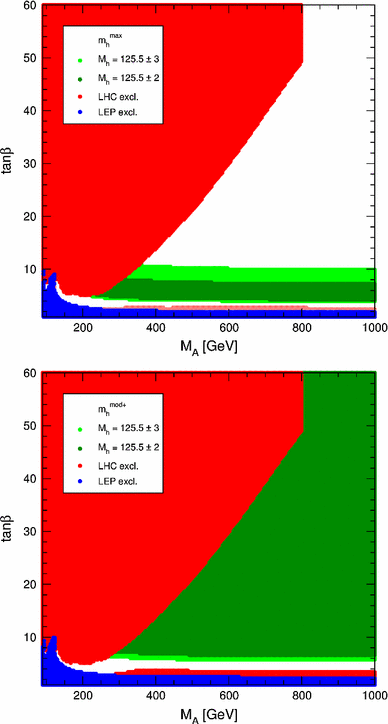

  

  $M_A$–$\tan \beta$ plane in the $m_h^{\max }$ scenario (upper) and in the $m_h^\mathrm{mod+}$ scenario (lower plot) [238]. The green-shaded area yields $M_h\sim 125 \pm 3 \,\mathrm {GeV}\,$, the red area at high $\tan \beta$ is excluded by LHC heavy MSSM Higgs-boson searches, the blue area is excluded by LEP Higgs searches, and the red strip at low $\tan \beta$ is excluded by the LHC SM Higgs searches

  In the lower plot of Fig. 61 we show the $m_h^\mathrm{mod+}$ scenario that differs from the $m_h^{\max }$ scenario in the choice of $X_t$. While in the $m_h^{\max }$ scenario $X_t/M_\mathrm{SUSY} = +2$ had been chosen to maximise $M_h$, in the $m_h^\mathrm{mod+}$ scenario $X_t/M_\mathrm{SUSY} = +1.5$ is used to yield a “good” $M_h$ value over the nearly the entire $M_A$–$\tan \beta$ plane, which is visible as the extended green region.

  Fig. 62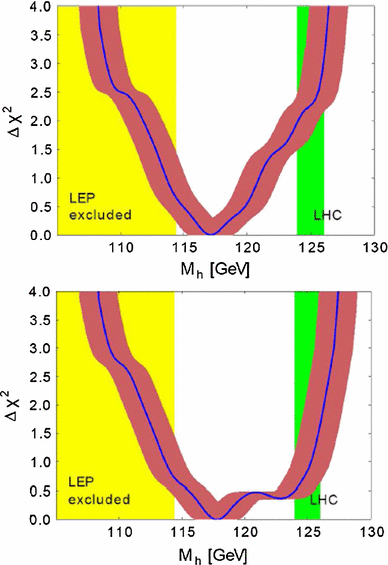

  

  Fit for the light ${\mathscr {CP}}$-even Higgs mass in the CMSSM (left) and NUHM1 (right) [254]. Direct searches for the light Higgs boson are not included

• In GUT based scenarios such as the CMSSM and the NUHM1¹³  it was shown that a light ${\mathscr {CP}}$-even Higgs boson around or slightly below $125\ \mathrm {GeV}\,$ is a natural prediction of these models [254]. These predictions take into account the current SUSY search limits (but no direct light Higgs search limits), as well as the relevant EWPO, B-physics observables and the relic Dark Matter density. In Fig. 62 we show the predictions in the CMSSM (upper) and the NUHM1 (lower plot). The red bands indicate a theory uncertainty of $\sim$1.5 GeV on the evaluation of $M_h$. The green columns indicate the range of the newly discovered particle mass.

• Parameter scans in the MSSM with 19 free parameters (pMSSM–19 [253]) are naturally compatible with a light Higgs boson around $M_h\sim 125\ \mathrm {GeV}\,$, as has been analysed in Refs. [255, 256] (see also Ref. [257] for a more recent analysis in the pMSSM–15 and Ref. [258] for an analysis in the pMSSM–19). Taking into account the available constraints from SUSY searches, Higgs searches, low-energy observables, B-physics observables and the relic abundance of Dark Matter viable scenarios can be identified that can be analysed in the upcoming LHC runs. Also the effects on the various production cross sections and branching ratios were analysed, where it was confirmed that light particles can modify in particular the decay rate to photons [239, 240].

  Fig. 63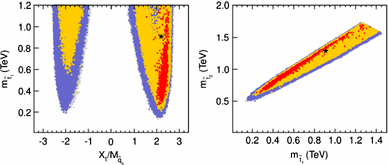

  

  Stop mixing parameter $X_t/m_{\tilde{q}_3}$ vs. the light stop mass (left), and the light vs. heavy stop masses (right), see text

• Parameter scans in the MSSM with seven free parameters (pMSSM–7) in comparison to the pMSSM–19 have the advantage of a full sampling of the parameter space with ${\mathscr {O}}(10^7)$ points; but they have the disadvantage of potentially not including all relevant phenomenogy of the MSSM. The pMSSM–7 fits to the full set of Higgs data (and several low-energy observables) [259] allow one to show an enhancement of the $\mathrm{BR}(h \rightarrow \gamma \gamma )$, correlated to a suppression of the decays to $b \bar{b}$ and $\tau ^+\tau ^-$ via the mechanisms outlined in Sect. 2.5.2 (see also Ref. [260]). In particular, these scans (while not incorporating the latest data) demonstrate that light scalar top masses are compatible with $M_h\sim 125\ \mathrm {GeV}\,$ (see also Ref. [248]). In Fig. 63 we show $X_t/m_{\tilde{q}_3}$ vs. the light stop mass (left plot, where $X_t= A_t- \mu /\tan \beta$ denotes the off-diagonal entry in the scalar top mass matrix, $A_t$ is the tri-linear Higgs-stop coupling, and $m_{\tilde{q}_3}$ denotes the (common) diagonal soft SUSY-breaking parameter in the scalar top and bottom sector) and the light vs. the heavy stop mass (right plot) in the case that the light ${\mathscr {CP}}$-even Higgs boson corresponds to the new state at $\sim$125 GeV. The coloured points passed the Higgs exclusion bounds (obtained using HiggsBounds [250–252]). The red (yellow) points correspond to the best-fit points with a ${\varDelta }\chi ^2 < 2.3 (5.99)$, see Ref. [259] for details. In the left plot one can see that the case of zero stop mixing in the MSSM is excluded by the observation of a light Higgs at $M_h\sim 125\ \mathrm {GeV}\,$ (unless $m_{\tilde{q}_3}$ is extremely large, see, e.g., Ref. [261]), and that values of $|X_t/m_{\tilde{q}_3}|$ between $\sim$1 and $\sim$2.5 must be realised. For the most favoured region we find $X_t/m_{\tilde{q}_3}= 2$– 2.5. Concerning the value of the lightest scalar top mass, the overall smallest values are found at $m_{\tilde{t}_1}\sim 200 \, \mathrm {GeV}\,$, where also the regions favoured by the fit to the Higgs rates start, in the case of $X_t$ positive. Such a light $\tilde{t}_{1}$ is accompanied by a somewhat heavier $\tilde{t}_{2}$, as can be seen in the right plot of Fig. 63. Values of $m_{\tilde{t}_1}\sim 200 \mathrm {GeV}\,$ are realised for $m_{\tilde{t}_2}\sim 600 \mathrm {GeV}\,$, which would mean that both stop masses are rather light, offering interesting possibilities for the LHC. The highest favoured $m_{\tilde{t}_1}$ values we find are $\sim$1.4 TeV. These are the maximal values reached in the scan in Ref. [259], but from Fig. 63 it is obvious that the favoured region extends to larger values of both stop masses. Such a scenario would be extremely difficult to access at the LHC.

Searches for the other Higgs bosons of the MSSM have so far not been successful. This applies to the heavy Higgs bosons of the MSSM as well as to a potentially light ${\mathscr {CP}}$-even Higgs bosons in the MSSM in the case that the new state at $\sim$125 GeV is interpreted as the heavy ${\mathscr {CP}}$-even Higgs boson, see Sect. 2.2.

2.5.4 Prospects for the MSSM Higgs bosons at the LHC

The prime task now is to study the properties of the discovered new particle and in particular to test whether the new particle is compatible with the Higgs boson of the SM or whether there are significant deviations from the SM predictions, which would point towards physics beyond the SM. A large part of the current and future LHC physics programme is devoted to this kind of analyses.

The prospects for the SM Higgs boson in this respect are the following [262–264]:

• The Higgs-boson mass can be determined down to a level of ${\mathscr {O}}(200\, \mathrm {MeV}\,)$.

• For the coupling determination the following has to be kept in mind. Since it is not possible to measure the Higgs production cross sections independently from the Higgs decay (or, equivalently, the Higgs boson width¹⁴), a determination of couplings is only possible if certain (theory) assumptions on the Higgs width are made, see, e.g. Ref. [196, 266]. For instance, it can be assumed that no new particles contribute to the decay width. Under this kind of assumption, going to the HL-LHC, precisions on couplings at the $\sim$10 % level can be achieved. Without any assumptions only ratios of couplings can be determined (see also Ref. [78] for a recent review).

• Studies in the context of the HL-LHC indicate that there might be some sensitivity on the tri-linear Higgs self-coupling; however, this will require a careful estimate of background contributions. Further studies to clarify these issues are currently in progress, see Ref. [267] for a discussion.

• It can be expected that the spin 2 hypothesis can be rejected using LHC data.

• A pure ${\mathscr {CP}}$-even state can be discarded at the $2\,\sigma$ level already from current data (assuming that the coupling strength to gauge bosons is the same one as in the ${\mathscr {CP}}$-even case). However, the prospects for the LHC to determine a certain level of ${\mathscr {CP}}$-odd admixture to the Higgs state are less clear [268].

In the case that the light ${\mathscr {CP}}$-even MSSM Higgs boson is identified with the new state at $\sim$125 GeV, as can be seen in Fig. 61, the decoupling region, $M_A\gg M_Z$ is a viable option. In this case the SM Higgs analyses can be taken over directly to the MSSM case – and will yield (nearly) identical results. Only light SUSY particles in the loops mediating the gluon fusion process or the decay to two photons might result in somewhat different predictions. However, depending on the actual values of the SUSY mass scales, these differences might easily remain unobservable with the anticipated LHC precision. Furthermore, in the decoupling regime the heavy MSSM Higgs bosons can easily be too heavy to be discovered at the LHC, in particular for medium or lower values of $\tan \beta$.

Only in the lower allowed range for $M_A$ in this scenario larger deviations from the phenomenology of the light ${\mathscr {CP}}$-even MSSM Higgs with respect to the SM Higgs can be expected. Depending on the level of decoupling, the LHC might be able to detect this kind of deviations, e.g. in enhanced rates involving the decay to two photons or in suppressed rates in the decay to $\tau$ leptons or b quarks.

2.5.5 Prospects for the MSSM Higgs bosons at the LC

As outlined in the previous subsection, identifying the light ${\mathscr {CP}}$-even Higgs with the new state at $\sim$125 GeV can easily result in a scenario where the LHC can neither distinguish the h from the SM Higgs boson, nor be able to discover additional Higgs bosons. In this case the analyses at an LC offer good prospects to reveal the non-SM nature of the Higgs particle. The anticipated experimental precisions for couplings to SM particles, the self-coupling etc., as given in detail in Sect. 2.3. In particular, the following improvements over the anticipated LHC precision/potential can be expected:

• The mass of a SM-like Higgs boson at $\sim$125 GeV can be determined at the level of $50 \mathrm {MeV}\,$.

• Using the Z recoil method the production cross section of a SM-like Higgs can be determined independently of the decay products, see Sect. 2.3. This allows for a model-independent measurement of the Higgs couplings at the per-cent level; see Table 18. In particular, a determination of the tri-linear Higgs self-coupling at the level of 15 % can be expected.

• The spin can be determined unambiguously from a production cross section threshold scan.

• The ${\mathscr {CP}}$ decomposition can be determined, in particular, using the channel $e^+e^- \rightarrow t \bar{t} H$ [270, 271].

• The reach for the heavy Higgs bosons can be extended to higher masses in particular for lower and intermediate values of $\tan \beta$ up to $M_A\lesssim \sqrt{s}/2$ (and possibly beyond, depending on the SUSY parameters [272]).

  An indirect determination of $M_A$ can be performed via a precise measurement of the Higgs couplings, where a sensitivity up to $800 \mathrm {GeV}\,$ was found [273].

  In the $\gamma \gamma$ option of the LC the Higgs bosons can be produced in the s-channel, and a reach up to $M_A\lesssim 0.8 \sqrt{s}$ can be realised [274] (see also Refs. [275, 276]).

Another measurement at the LC can turn out to be crucial for Higgs physics in the MSSM: the determination of $m_{t}\,$ from a threshold scan. As can be seen in Eq. (30), the theory prediction of $M_h$ depends strongly on $m_{t}\,$. Only the LC determination of a well-defined top-quark mass can yield a theory prediction that matches the LHC precision in $M_h$. More details can be found in Sect. 4.4.

2.6 General multi-Higgs structures¹⁵

2.6.1 Introduction

We here give a review of extended Higgs sectors and their collider phenomenology. In the SM, one isospin doublet scalar field $\Phi$ is simply introduced as the minimum form. Under the requirement of the renormalisability its potential can be uniquely written as

$$\begin{aligned} V(\Phi ) = + \mu ^2 |\Phi |^2 + \lambda |\Phi |^4. \end{aligned}$$

(31)

Table 18 Examples of the precision of SM-like Higgs observables at a $\sqrt{s}=500 \mathrm {GeV}\,$ LC assuming a Higgs-boson mass of $125 \, \mathrm {GeV}\,$. The results are based on the ILC set-up. For the direct measurements, an integrated luminosity of ${\mathscr {L}}^\mathrm{int} = 500~\mathrm {fb}^{-1}$ is assumed. For the indirect measurements at GigaZ, a running time of approximately one year is assumed, corresponding to ${\mathscr {L}}=$ ${\mathscr {O}}(10~\mathrm {fb}^{-1})$. Taken from Ref. [269]

By putting an assumption of $\mu ^2 < 0$ (and $\lambda > 0$), the shape of the potential becomes like a Mexican hat, and the electroweak symmetry is broken spontaneously at the vacuum $\langle \Phi \rangle = (0, v/\sqrt{2})^T$. Consequently, weak gauge bosons, quarks and charged leptons obtain their masses from the unique vacuum expectation value (VEV) v ($=(\sqrt{2}G_F)^{-1/2} \simeq 246$ GeV). However, there is no theoretical principle for the SM Higgs sector, and there are many possibilities for non-minimal Higgs sectors. While the current LHC data do not contradict the predictions of the SM, most of the extended Higgs sectors can also satisfy current data. These extended Higgs sectors are often introduced to provide physics sources to solve problems beyond the SM, such as baryogenesis, DM and tiny neutrino masses. Each scenario can predict a specific Higgs sector with additional scalars.

It is also known that the introduction of the elementary scalar field is problematic from the theoretical viewpoint, predicting the quadratic divergence in the radiative correction to the mass of the Higgs boson. Such a quadratic divergence causes the hierarchy problem. There are many scenarios proposed to solve the hierarchy problem such as supersymmetry, dynamical symmetry breaking, Extra dimensions and so on. Many models based on these new paradigms predict specific Higgs sectors in their low-energy effective theories.

Therefore, experimental determination of the structure of the Higgs sector is essentially important to deeply understand EWSB and also to find direction to new physics beyond the SM. The discovery of the 125-GeV Higgs boson at the LHC in 2012 is a big step to experimentally investigate the structure of the Higgs sector. From the detailed study of the Higgs sector, we can determine the model of new physics.

What kind of extended Higgs sectors can we consider? As the SM Higgs sector does not contradict the current data within the errors, there should be at least one isospin doublet field which looks like the SM Higgs boson. An extended Higgs sector can then contain additional isospin multiplets. There can be infinite kinds of extended Higgs sectors. These extended Higgs sectors are subject to constraints from the current data of many experiments including those of the electroweak $\rho$-parameter and for flavour changing neutral currents (FCNCs).

The electroweak $\rho$-parameter is calculated at the tree level for a Higgs sector with N multiplets by

$$\begin{aligned} \rho = \frac{m_W^2}{m_Z^2 \cos ^2\theta _W} = \frac{\sum _i \left\{ 4 T_i (T_i+1)- Y_i^2 \right\} |v_i|^2 c_i}{\sum _i 2 Y_i^2 |v_i|^2}, \end{aligned}$$

(32)

where $T_i$ and $Y_i$ ($i=1, \ldots , N$) are isospin and hypercharges of the ith multiplet field ($Q_i=T_i+Y_i/2$), and $c_i =1/2$ for real fields ($Y_i=0$) and 1 for complex fields. The data shows that $\rho =1.0004^{+0.0003}_{-0.0004}$ [277]. Higgs sectors with additional doublets $(T_i, Y_i) = (1/2, 1)$ (and singlets with $Y_i=0$) predict $\rho =1$ at the tree level, like the SM Higgs sector. Thus, multi-doublet structures would be a natural extension of the Higgs sector. The introduction of higher representation fields generally causes a tree-level deviation in the $\rho$- parameter from unity. For example, in the model with a triplet field ${\varDelta }$(1, 2) with the VEV $v_{\varDelta }$, $\rho \sim 1 - 2(v_{\varDelta }/v)^2$ is given, so that in such a model a tuning $(v_{\varDelta }/v)^2 \ll 1$ is required to satisfy the data. We note that there are exceptional Higgs sectors with larger isospin representations which predict $\rho =1$ at the tree level. In the model proposed by Georgi and Machacek [278], the Higgs sector is composed of an isospin doublet field with additional a complex (1, 2) and a real (1, 0) triplet fields, which satisfies $\rho =1$ at the tree level. Addition of the septet field (3, 2) to the SM Higgs sector also predicts $\rho =1$ at the tree level.

Extended Higgs sectors with a multi-doublet structure, in general, receive a severe constraint from the results of FCNC experiments. The data show that FCNC processes such as $K^0 \rightarrow \mu ^+\mu ^-$, $B^0-\bar{B}^0$ and so on are highly suppressed [277]. In the SM with a doublet Higgs field, the suppression of FCNC processes is perfectly explained by the so-called Glashow–Illiopoulos–Miani mechanism [

References

F. Englert, R. Brout, Phys. Rev. Lett. 13, 321 (1964)
P.W. Higgs, Phys. Lett. 12, 132 (1964)
P.W. Higgs, Phys. Rev. Lett. 13, 508 (1964)
G.S. Guralnik, C.R. Hagen, T.W.B. Kibble, Phys. Rev. Lett. 13, 585 (1964)
T. Schörner-Sadenius, The Large Hadron Collider: Harvest of Run 1 (Springer, New York, 2015). ISBN-10:3319150006, ISBN-13:978–3319150000
M. Lamont, EPS, in LHC, HL-LHC and Beyond, Proceedings, Stockholm (2013)
J.A. Aguilar-Saavedra et al. [ECFA/DESY LC Physics Working Group Collaboration]. arXiv:hep-ph/0106315
H. Baer et al., Physics Chapter of the ILC Detailed Baseline Design Report. ILC-INT-2012-053. arXiv:1306.6352
L. Linssen, A. Miyamoto, M. Stanitzki, H. Weerts. arXiv:1202.5940 [physics.ins-det]
P. Lebrun, L. Linssen, A. Lucaci-Timoce, D. Schulte, F. Simon, S. Stapnes, N. Toge, H. Weerts et al. arXiv:1209.2543
R.D. Heuer et al., Parameters for the Linear Collider. http://ilc-edmsdirect.desy.de/ilc-edmsdirect/file.jsp?edmsid=*948205. Accessed 20 Nov 2006. (Prepared by the parameters sub-panel of the International Linear Collider Steering Committee)
T. Abe et al. [American Linear Collider Working Group Collaboration]. arXiv:hep-ex/0106056
T. Abe et al. [American Linear Collider Working Group Collaboration]. arXiv:hep-ex/0106055
T. Abe et al. [American Linear Collider Working Group Collaboration]. arXiv:hep-ex/0106057
T. Abe et al. [American Linear Collider Working Group Collaboration]. arXiv:hep-ex/0106058
K. Abe et al. [ACFA Linear Collider Working Group Collaboration]. arXiv:hep-ph/0109166
J. Brau, R. Godbole, F. LeDiberder, M. Thomson, H. Weerts, G. Weiglein, J. Wells, H. Yamamoto, LC-REP-2012-071. http://www-flc.desy.de/lcnotes/. arXiv:1210.0202
E. Avrile et al., Dark matter results from 225 live days of XENON100 data. Phys. Rev. Lett. 109, 181301 (2012)
N. Okabe et al., LoCuSS: The mass density profile of massive galaxy clusters at \(z = 0.2\). 769(2) (2013). (Article ID 35)
R. Kallosh, A. Linde, A. Westphal. arXiv:1405.0270 [hep-th]
S. Schael et al., Phys. Rept. 427, 257 (2006). http://lepewwg.web.cern.ch/LEPEWWG/. arXiv:hep-ex/0509008
G.W. Bennett et al. [Muon \((g-2)\) Collaboration], Phys. Rev. D 73, 072003 (2006)
D.W. Hertzog, B. Lee Roberts et al., Fermilab proposal P-989 (2009). http://www.fnal.gov/directorate/program_planning/Mar2009PACPublic/PACMarch09AgendaPublic.htm. Accessed March 2009
T. Mibe, Chin. Phys. C 34, 745–748 (2010)
M. Tigner, Nuovo Cim. 37, 1228 (1965)
U. Amaldi, Phys. Lett. B 61, 313 (1976)
LCC Parameter Group, ILC Running Scenarios, T. Barklow, J. Brau, K. Fujii, J. Gao, J. List, N. Walker, K. Yokoya. arXiv:1506.07830
K. Fujii et al. arXiv:1506.05992 [hep-ex]
S. Dawson, A. Gritsan, H. Logan, J. Qian, C. Tully, R.V. Kooten et al., Snowmass Higgs working group report (2013). arXiv:1310.8361
G. Moortgat-Pick, I. Fleck, S. Riemann, F. Simon, O.S. Adeyemi, G. Alexander, M.S. Amjad, V.V. Andreev et al., DESY 12–123H (2013). doi:10.3204/DESY_12-123H
Linear Collider Notes. http://www-flc.desy.de/lcnotes/
A. Denner, S. Heinemeyer, I. Puljak, D. Rebuzzi, M. Spira, Eur. Phys. J. C 71, 1753 (2011).arXiv:1107.5909 [hep-ph]
S. Liebler, G. Moortgat-Pick, G. Weiglein, Off-shell effects in Higgs processes at a linear collider and implications for the LHC, DESY 14–133. arXiv:1502.07970 [hep-ph]
F. Caola, K. Melnikov, Phys. Rev. D 88, 054024 (2013)
J.S. Gainer, J. Lykken, K.T. Matchev, S. Mrenna, M. Park, Phys. Rev. D 91(3), 035011 (2015). arXiv:1403.4951 [hep-ph]
M. Ghezzi, G. Passarino, S. Uccirati, PoS LL 2014, 072 (2014).arXiv:1405.1925 [hep-ph]
A. David et al. [LHC Higgs Cross Section Working Group Collaboration]. arXiv:1209.0040 [hep-ph]
S. Heinemeyer et al. [LHC Higgs Cross Section Working Group Collaboration]. arXiv:1307.1347 [hep-ph]
P. Bechtle, S. Heinemeyer, O. Stål, T. Stefaniak, G. Weiglein, JHEP 1411, 039 (2014).arXiv:1403.1582 [hep-ph]
K. Seidel, F. Simon, M. Tesar, S. Poss, Eur. Phys. J. C 73, 2530 (2013).arXiv:1303.3758 [hep-ex]
M.S. Amjad, T. Frisson, E. Kou, R. Poschl, F. Richard, J. Rouene, Nuovo Cim. C 037(02), 55 (2014)
A. Juste et al. [Report of the 2005 Snowmass Top/QCD Working Group], econf/C0508141:PLEN0043 (2005). arXiv:hep-ph/0601112
S.Y. Choi, J. Kalinowski, G.A. Moortgat-Pick, P.M. Zerwas, Eur. Phys. J. C 22, 563 (2001)
S.Y. Choi, J. Kalinowski, G.A. Moortgat-Pick, P.M. Zerwas, Eur. Phys. J. C 23, 769 (2002). arXiv:hep-ph/0108117
G. Moortgat-Pick, T. Abe, G. Alexander, B. Ananthanarayan, A.A. Babich, V. Bharadwaj, D. Barber, A. Bartl et al., Phys. Rep. 460, 131 (2008). arXiv:hep-ph/0507011
G. Hinshaw et al. [WMAP Collaboration], Astrophys. J. Suppl. 208, 19 (2013). arXiv:1212.5226 [astro-ph.CO]
P.A.R. Ade et al. [Planck Collaboration]. arXiv:1303.5076 [astro-ph.CO]
A. Birkedal, K. Matchev, M. Perelstein, Phys. Rev. D 70, 077701 (2004). arXiv:hep-ph/0403004
C. Bartels, M. Berggren, J. List, Eur. Phys. J. C 72, 2213 (2012).arXiv:1206.6639 [hep-ex]
H. Dreiner, M. Huck, M. Krämer, D. Schmeier, J. Tattersall, Phys. Rev. D 87(7), 075015 (2013). arXiv:1211.2254 [hep-ph]
D. Schmeier. arXiv:1308.4409 [hep-ph]
B. Vormwald, J. List, Eur. Phys. J. C 74, 2720 (2014).arXiv:1307.4074 [hep-ex]
W. Porod, M. Hirsch, J. Romao, J.W.F. Valle, Phys. Rev. D 63, 115004 (2001). arXiv:hep-ph/0011248
M. Hirsch, W. Porod, Phys. Rev. D 68, 115007 (2003). arXiv:hep-ph/0307364
J. Brau (ed.) [ILC Collaboration]. arXiv:0712.1950 [physics.acc-ph]
G. Aarons et al. [ILC Collaboration], The ILC. arXiv:0709.1893 [hep-ph]
P.W. Higgs, Phys. Rev. 145, 1156 (1966)
S.L. Glashow, Nucl. Phys. 22, 579 (1961)
A. Salam, Conf. Proc. C 680519, 367 (1968)
S. Weinberg, Phys. Rev. Lett. 19, 1264 (1967)
ATLAS Collaboration, Phys. Lett. B 716, 1 (2012). arXiv:1207.7214 [hep-ex]
CMS Collaboration, Phys. Lett. B 716, 30 (2012). arXiv:1207.7235 [hep-ex]
ATLAS Collaboration, ATLAS-CONF-2014-009
CMS Collaboration, CMS-PAS-HIG-14-009
ATLAS Collaboration, Phys. Lett. B 726, 120 (2013). arXiv:1307.1432 [hep-ex]
CMS Collaboration, Phys. Rev. Lett. 110, 081803 (2013). arXiv:1212.6639 [hep-ex]
J.R. Ellis, M.K. Gaillard, D.V. Nanopoulos, Nucl. Phys. B 106, 292 (1976)
B.L. Ioffe, V.A. Khoze, Sov. J. Part. Nucl. 9, 50 (1978). [Fiz. Elem. Chast. Atom. Yadra 9, 118 (1978)]
D.R.T. Jones, S.T. Petcov, Phys. Lett. B 84, 440 (1979)
R.N. Cahn, S. Dawson, Phys. Lett. B 136, 196 (1984). [Erratum-ibid. B 138, 464 (1984)]
W. Kilian, M. Kramer, P.M. Zerwas, Phys. Lett. B 373, 135 (1996). arXiv:hep-ph/9512355
ALEPH, DELPHI, L3 and OPAL Collaborations, The LEP working group for Higgs boson searches. Phys. Lett. B 565, 61 (2003)
W.D. Schlatter, P.M. Zerwas, Eur. Phys. J. H 36, 579 (2012).arXiv:1112.5127 [physics.hist-ph]
N. Cabibbo, L. Maiani, G. Parisi, R. Petronzio, Nucl. Phys. B 158, 295 (1979)
M. Sher, Phys. Rep. 179, 273 (1989)
G. Degrassi, S. Di Vita, J. Elias-Miro, J.R. Espinosa, G.F. Giudice, G. Isi dori, A. Strumia, JHEP 1208, 098 (2012). arXiv:1205.6497 [hep-ph]
V.D. Barger, K.-M. Cheung, A. Djouadi, B.A. Kniehl, P.M. Zerwas, Phys. Rev. D 49, 79 (1994). arXiv:hep-ph/9306270
C. Englert, A. Freitas, M. Muhlleitner, T. Plehn, M. Rauch, M. Spira, K. Walz, Physics scales. J. Phys. G 41, 113001 (2014).arXiv:1403.7191 [hep-ph]
A. Djouadi, W. Kilian, M. Muhlleitner, P.M. Zerwas, Eur. Phys. J. C 10, 27 (1999). arXiv:hep-ph/9903229
T. Binoth, J.J. van der Bij, Z. Phys. C 75, 17 (1997). arXiv:hep-ph/9608245
B. Patt, F. Wilczek. arXiv:hep-ph/0605188
Y.A. Golfand, E.P. Likhtman, JETP Lett. 13, 323 (1971). [Pisma Zh. Eksp. Teor. Fiz. 13, 452 (1971)]
J. Wess, B. Zumino, Nucl. Phys. B 70, 39 (1974)
J.F. Gunion, H.E. Haber, Nucl. Phys. B 272, 1 (1986). [Erratum-ibid. B 402, 567 (1993)]
J.F. Gunion, H.E. Haber, Nucl. Phys. B 278, 449 (1986)
J.F. Gunion, H.E. Haber, G.L. Kane, S. Dawson, Front. Phys. 80, 1 (2000)
A. Djouadi, Phys. Rep. 459, 1 (2008). arXiv:hep-ph/0503173
P. Fayet, S. Ferrara, Phys. Rep. 32, 249 (1977)
U. Ellwanger, C. Hugonie, A.M. Teixeira, Phys. Rep. 496, 1 (2010).arXiv:0910.1785 [hep-ph]
S. Weinberg, Phys. Rev. D 13, 974 (1976)
L. Susskind, Phys. Rev. D 20, 2619 (1979)
T. Han, H.E. Logan, L.-T. Wang, JHEP 0601, 099 (2006). arXiv:hep-ph/0506313
J.R. Espinosa, C. Grojean, M. Muhlleitner, EPJ Web Conf. 28, 08004 (2012).arXiv:1202.1286 [hep-ph]
ATLAS Collaboration, Phys. Lett. B 716, 1 (2012)
ATLAS Collaboration, Science, 338(6114), 1576–1582 (2012)
CMS Collaboration, JHEP 1306, 081 (2013)
S. Dittmaier et al. [LHC Higgs Cross Section Working Group Collaboration]. arXiv:1101.0593 [hep-ph]
S. Dittmaier et al. [LHC Higgs Cross Section Working Group Collaboration]. arXiv:1201.3084 [hep-ph]
ATLAS Collaboration, Phys. Lett. B 710, 49 (2012)
C.M.S. Collaboration, Phys. Lett. B 710, 26 (2012)
ATLAS Collaboration, Phys. Rev. D 90, 112015 (2014)
CMS Collaboration, Phys. Rev. D 89, 092007 (2014)
ATLAS Collaboration. arXiv:1412.2641 [hep-ex]. (submitted to Phys. Rev. D)
C.M.S. Collaboration, Eur. Phys. J. C 74(10), 3076 (2014)
ATLAS Collaboration, Phys. Rev. D 91, 012006 (2015)
CMS Collaboration, JHEP 1401, 096 (2014)
ATLAS Collaboration, JHEP 01, 069 (2015)
CMS Collaboration, Phys. Rev. D 89(1), 012003 (2014)
CMS Collaboration, JHEP 1405, 104 (2014)
ATLAS Collaboration. arXiv:1501.04943 [hep-ex]. (submitted to JHEP)
CMS Collaboration, Nat. Phys. 10, 557 (2014)
ATLAS Collboration, ATLAS-CONF-2015-007
CMS Collaboration. arXiv:1412.8662 [hep-ex]. (submitted to Eur. Phys. J. C)
ATLAS Collaboration, Phys. Rev. D 90, 052004 (2014)
ATLAS Collaboration. arXiv:1503.01060 [hep-ex]. (submitted to Eur. Phys. J. C)
CMS Collaboration, Phys. Lett. B 736, 64 (2014)
CMS Collaboration. arXiv:1411.3441 [hep-ex]. (submitted to Phys. Rev. D)
ATLAS Collaboration. arXiv:1503.03643 [hep-ex]. (submitted to Eur. Phys. J. C)
ATLAS Collaboration, ATLAS-CONF-2015-008
ATLAS and CMS Collaborations, Contribution to Rencontres de Moriond 2015 – EW Interactions and Unified Theories
N. Kauer, G. Passarino, JHEP 1208, 116 (2012)
C. Englert, M. Spannowsky, Phys. Rev. D 90, 053003 (2014)
ATLAS Collaboration, JHEP 1409, 112 (2014)
ATLAS Collaboration, Phys. Lett. B 738, 234 (2014)
ATLAS Collaboration, Phys. Lett. B 738, 68 (2014)
CMS Collaboration. arXiv:1410.6679 [hep-ex]. (submitted to Phys. Lett. B)
ATLAS Collaboration, Phys. Lett. B 732, 8 (2014)
CMS Collaboration, Phys. Lett. B 726, 587 (2013)
ATLAS Collaboration. arXiv:1501.03276 [hep-ex]
ATLAS Collaboration, Phys. Rev. Lett. 112, 201802 (2014)
CMS Collaboration, Eur. Phys. J. C 74(8), 2980 (2014)
ATLAS Collaboration, Phys. Lett. B 740, 222 (2015)
CMS Collaboration, JHEP 1409, 087 (2014). [Erratum-ibid. 1410, 106 (2014)]
CMS Collaboration. arXiv:1502.02485 [hep-ex]. (submitted to Eur. Phys. J. C)
ATLAS Collaboration. arXiv:1503.05066 [hep-ex]. (submitted to Eur. Phys. J. C)
ATLAS Collaboration, ATL-PHYS-PUB-2014-016
CMS Collaboration, CMS-NOTE-2013-002. arXiv:1307.7135 [hep-ex]
ATLAS Collaboration, ATL-PHYS-PUB-2013-014
ATLAS Collaboration, ATL-PHYS-PUB-2014-019
http://www-jlc.kek.jp/subg/physics/ilcphys/. Accessed 20 July 2015
D.M. Asner et al. (2013). arXiv:1310.0763 [hep-ph]. arXiv:hep-ph/0406323
ATLAS, Phys. Lett. B 716, 1–29 (2012)
CMS, Phys. Lett. B 716, 30–61 (2012)
ACFA Liner Collider WG, K. Abe et al. (2002). arXiv:hep-ph/0109166
L.J. Hall, M.B. Wise, Nucl. Phys. B 187, 397 (1981)
M. Aoki, S. Kanemura, K. Tsumura, K. Yagyu, Phys. Rev. D 80, 015017 (2009)
Physics Volume of the ILC Technical Design Report (2013)
G. Degrassi et al., JHEP 1208, 098 (2012). arXiv:1205.6497 [hep-ph]
F. Bezrukov et al., JHEP 1210, 140 (2012).arXiv:1205.2893 [hep-ph]
S. Kawada et al., Phys. Rev. D 85, 113009 (2012)
S. Watanuki, in Presentation at LCWS’13, Tokyo, 2013
C. Englert, T. Plehn, D. Zerwas, P.M. Zerwas, Phys. Lett. B 703, 298–305 (2011)
A. Yamamoto, A. Ishikawa, in Presentation at the Asian Physics and Software Meeting (2012)
A. Yamamoto, A. Ishikawa [ATLAS Collabration], Phys. Lett. B 726, 120–144 (2013)
A. Yamamoto, A. Ishikawa [CMS], Phys. Rev. D 89, 092007 (2014)
M.T. Dova, P. Garcia-Abia, W. Lohmann (2003). arXiv:hep-ph/0302113
D.J. Miller, S.Y. Choi, B. Eberle, M.M. Muhlleitner, P.M. Zerwas, Phys. Lett. B 505, 149 (2001). arXiv:hep-ph/0102023
M. Schumacher, LC-PHSM-2001-003 (2001)
M. Kramer, J.H. Kuhn, M.L. Stong, P.M. Zerwas, Z. Phys. C 64, 21 (1994). arXiv:hep-ph/9404280
S. Berge, W. Bernreuther, H. Spiesberger (2012). arXiv:1208.1507 [hep-ph]
K. Desch, A. Imhof, Z. Was, M. Worek, Phys. Lett. B 579, 157 (2004). arXiv:hep-ph/0307331
H. Ono, A. Miyamoto, Eur. Phys. J. C73, 2343 (2013)
Y. Banda, T. Lastovicka, A. Nomerotski, Phys. Rev. D 82, 033013 (2010)
H. Ono, in Presentation at KILC2012 Workshop (Daegu, 2012)
S. Kawada, K. Fujii, T. Suehara, T. Takahashi, T. Tanabe, LC-REP-2013-001 (2013)
S. Kawada, K. Fujii, T. Suehara, T. Takahashi, T. Tanabe (2013).arXiv:1308.5489 [hep-ph]
E. Boos, J.C. Brient, D.W. Reid, H.J. Schreiber, R. Shanidze, Eur. Phys. J. C 19, 455–461 (2001)
T. Kuhl, K. Desch, LC-PHSM-2007-2 (2007)
C. Calancha, in Presentation at LCWS2013, Tokyo, 2013
C. Dürig, in Presentation at LCWS12, Arlington, 2012
J. Tian, C. Duerig, K. Fujii, J. List, LC-REP-2013-022 (2013)
A. Djouadi, J. Kalinowski, P.M. Zerwas, Z. Phys. C 54, 255 (1992)
S. Dittmaier, M. Kramer, Y. Liao, M. Spira, P.M. Zerwas, Phys. Lett. B 441, 383 (1998). arXiv:hep-ph/9808433
H. Baer, S. Dawson, L. Reina, Phys. Rev. D 61, 013002 (2000)
S. Dawson, L. Reina, Phys. Rev. D 59, 054012 (1999). arXiv:hep-ph/9808443
G. Belanger, F. Boudjema, J. Fujimoto, T. Ishikawa, T. Kaneko, K. Kato, Y. Shimizu, Y. Yasui, Phys. Lett. B 571, 163 (2003). arXiv:hep-ph/0307029
A. Denner, S. Dittmaier, M. Roth, M.M. Weber, Nucl. Phys. B 680, 85 (2004). arXiv:hep-ph/0309274
Y. You, W.G. Ma, H. Chen, R.Y. Zhang, S. Yan-Bin, H.S. Hou, Phys. Lett. B 571, 85 (2003). arXiv:hep-ph/0306036
C. Farrell, A.H. Hoang, Phys. Rev. D 72, 014007 (2005). arXiv:hep-ph/0504220
C. Farrell, A.H. Hoang, Phys. Rev. D 74, 014008 (2006). arXiv:hep-ph/0604166
R. Yonamine et al., Phys. Rev. D 84, 014033 (2011)
H. Tabassam, V. Martin (2012). arXiv:hep-ph/1202.6013
ILD and SiD Analyses in Detailed Baseline Design Report in ILC TDR (2013)
A. Juste, G. Merino (1999). arXiv:hep-ph/9910301
A. Gay, Eur. Phys. J. C 49, 489 (2007). arXiv:hep-ph/0604034
J. Tian, Higgs self-coupling, contribution to the ‘Helmholtz Alliance Linear Collider Forum: Proceedings of the Workshops Hamburg, Munich, Hamburg 2010-2012, Germany’, LC note LC-REP-2013-003 (2013). http://flc.desy.de/lcnotes/index_eng.html
C. Castanier, P. Gay, P. Lutz, J. Orloff (2001). arXiv:hep-ex/0101028
M. Battaglia, E. Boos, W.M. Yao, eConf C 010630, E3016 (2001). arXiv:hep-ph/0111276
Y. Yasui, S. Kanemura, S. Kiyoura, K. Odagiri, Y. O kada, E. Senaha, S. Yamashita (2002). arXiv:hep-ph/0211047
S. Yamashita, in Presentation at LCWS04 (2004)
T.L. Barklow (2003). arXiv:hep-ph/0312268
M. Kurata, T. Tanabe, J. Tian, K. Fujii, T. Suehara, LC-REP-2013-025 (2013)
T. Price, T. Tanabe, K. Fujii, V. Martin, N. Watson, LC-REP-2013-004 (2013)
M. Battaglia, A. De Roeck, eConf C 010630, E3066 (2001). arXiv:hep-ph/0111307
J. Tian, K. Fujii, LC-REP-2013-021 (2013)
M. Dührssen, S. Heinemeyer, H. Logan, D. Rainwater, G. Weiglein, D. Zeppenfeld, Phys. Rev. D 70, 113009 (2004). arXiv:hep-ph/0406323
M. Peskin. arXiv:1207.2516 [hep-ph]
D. Zerwas, in The presentation at LCWS12, Texas, 2012
R.S. Gupta et al. arXiv:1206.3560 [hep-ph]
S. Kanemura, K. Tsumura, K. Yagyu, H. Yokoya (2014). arXiv:1406.3294 [hep-ph]
ILC Technical Design Report (2013)
ILC, RDR (2007). http://www.linearcollider.org/ILC/Publications/Reference-Design-Report. arXiv:0712.2361
M. Aicheler, P. Burrows, M. Draper, T. Garvey, P. Lebrun, K. Peach, N. Phinney et al., gn Report, CERN-2012-007
T. Behnke, J.E. Brau, B. Foster, J. Fuster, M. Harrison, J.M. Paterson, M. Peskin, M. Stanitzki et al. arXiv:1306.6327
H. Aihara et al. [SiD Collaboration], SiD Letter of Intent, SLAC-R-944
T. Behnke, J.E. Brau, P.N. Burrows, J. Fuster, M. Peskin, M. Stanitzki, Y. Sugimoto, S. Yamada et al. arXiv:1306.6329 [physics.ins-det]
T. Abe et al. [ILD Concept Group - Linear Collider Collaboration],arXiv:1006.3396 [hep-ex]
H. Abramowicz et al. [CLIC Detector and Physics Study Collaboration], arXiv:1307.5288 [hep-ex]
[ATLAS Collaboration], ATLAS-CONF-2013-014
[CMS Collaboration], CMS-PAS-HIG-13-005
F. Gianotti, M.L. Mangano, T. Virdee, S. Abdullin, G. Azuelos, A. Ball D. Ba rberis and A. Belyaev et al. D. Ba rberis and A. Belyaev, et al., Eur. Phys. J. C 39, 293 (2005). arXiv:hep-ph/0204087
E. Coniavitis and A. Ferrari, Phys. Rev. D 75 (2007) 015004. Combined measurements of the mass and signal strength of the Higgs-like boson with the ATLAS detector using up to 25 fb\(^{-1}\) of proton-proton collision data, ATLAS-CONF-2013-014
M. Battaglia, N. Kelley, B. Hooberman, Phys. Rev. D 78, 015021 (2008)
A. Pilaftsis, C. Wagner, Nucl. Phys. B 553, 3 (1999). arXiv:hep-ph/9902371
M. Frank, T. Hahn, S. Heinemeyer, W. Hollik, R. Rzehak, G. Weiglein, JHEP 0602, 047 (2007). arXiv:hep-ph/0611326
H.P. Nilles, Phys. Rept. 110, 1 (1984)
H.E. Haber, G.L. Kane, Phys. Rept. 117, 75 (1985)
R. Barbieri, Riv. Nuovo Cim. 11, 1 (1988)
H. E. Haber, arXiv:hep-ph/9501320
J.F. Gunion, H.E. Haber, Phys. Rev. D 67, 075019 (2003). arXiv:hep-ph/0207010
A. Djouadi, Phys. Rept. 459, 1 (2008). arXiv:hep-ph/0503173
S. Heinemeyer, Int. J. Mod. Phys. A 21, 2659 (2006). arXiv:hep-ph/0407244
J. Ellis, G. Ridolfi, F. Zwirner, Phys. Lett. B 257, 83 (1991)
Y. Okada, M. Yamaguchi, T. Yanagida, Prog. Theor. Phys. 85, 1 (1991)
H. Haber, R. Hempfling, Phys. Rev. Lett. 66, 1815 (1991)
G. Degrassi, S. Heinemeyer, W. Hollik, P. Slavich, G. Weiglein, Eur. Phys. J. C 28, 133 (2003). arXiv:hep-ph/0212020
O. Buchmueller et al., Eur. Phys. J. C 74, 2809 (2014).arXiv:1312.5233 [hep-ph]
S. Heinemeyer, W. Hollik, G. Weiglein, Eur. Phys. J. C 16, 139 (2000). arXiv:hep-ph/0003022
M. Carena, S. Heinemeyer, C. Wagner, G. Weiglein, Eur. Phys. J. C 26, 601 (2003). arXiv:hep-ph/0202167
R. Hempfling, Phys. Rev. D 49, 6168 (1994)
L. Hall, R. Rattazzi, U. Sarid, Phys. Rev. D 50, 7048 (1994). arXiv:hep-ph/9306309
M. Carena, M. Olechowski, S. Pokorski, C. Wagner, Nucl. Phys. B 426, 269 (1994). arXiv:hep-ph/9402253
M. Carena, D. Garcia, U. Nierste, C. Wagner, Nucl. Phys. B 577, 577 (2000). arXiv:hep-ph/9912516
D. Noth, M. Spira, Phys. Rev. Lett. 101, 181801 (2008).arXiv:0808.0087 [hep-ph]
M. Carena, S. Heinemeyer, C. Wagner, G. Weiglein, Eur. Phys. J. C 45, 797 (2006). arXiv:hep-ph/0511023
S. Gennai, S. Heinemeyer, A. Kalinowski, R. Kinnunen, S. Lehti, A. Nikitenko, G. Weiglein, Eur. Phys. J. C 52, 383 (2007).arXiv:0704.0619 [hep-ph]
A. Djouadi, Phys. Lett. B 435, 101 (1998). arXiv:hep-ph/9806315
M. Carena, S. Heinemeyer, O. Stål, C. Wagner, G. Weiglein, Eur. Phys. J. C 73, 2552 (2013).arXiv:1302.7033 [hep-ph]
M. Carena, S. Gori, N.R. Shah, C.E.M. Wagner, JHEP 1203, 014 (2012).arXiv:1112.3336 [hep-ph]
M. Carena, S. Gori, N. R. Shah, C. E. M. Wagner and L. -T. Wang, arXiv:1205.5842 [hep-ph]
G. Aad et al., ATLAS Collaboration. Phys. Lett. B 716, 1 (2012).arXiv:1207.7214 [hep-ex]
S. Chatrchyan et al., CMS Collaboration. Phys. Lett. B 716, 30 (2012).arXiv:1207.7235 [hep-ex]
CDF Collaboration, DØ Collaboration, arXiv:1207.0449 [hep-ex]
E. Gross, talk given at Moriond Electroweak, March 2014, see: URL: https://indico.in2p3.fr/event/9116
P. Musella, talk given at Moriond Electroweak, March 2014, see: URL: https://indico.in2p3.fr/event/9116
B. de Micco, talk given at Moriond QCD, March 2014, see: URL: http://moriond.in2p3.fr/QCD/2014
N. de Filippis, talk given at Moriond QCD, March 2014, see: URL: http://moriond.in2p3.fr/QCD/2014
S. Heinemeyer, O. Stål, G. Weiglein, Phys. Lett. B 710, 201 (2012).arXiv:1112.3026 [hep-ph]
ATLAS Collaboration, ATLAS-CONF-2013-090
P. Bechtle, O. Brein, S. Heinemeyer, G. Weiglein, K.E. Williams, Comput. Phys. Commun. 181, 138 (2010).arXiv:0811.4169 [hep-ph]
P. Bechtle, O. Brein, S. Heinemeyer, G. Weiglein, K.E. Williams, Comput. Phys. Commun. 182, 2605 (2011).arXiv:1102.1898 [hep-ph]
P. Bechtle, O. Brein, S. Heinemeyer, O. Stål, T. Stefaniak, G. Weiglein, K. Williams, Eur. Phys. J. C 74, 2693 (2014).arXiv:1311.0055 [hep-ph]
S.S. AbdusSalam et al., Eur. Phys. J. C 71, 1835 (2011).arXiv:1109.3859 [hep-ph]
O. Buchmueller et al., Eur. Phys. J. C 72, 2243 (2012).arXiv:1207.7315 [hep-ph]
A. Arbey, M. Battaglia, F. Mahmoudi, Eur. Phys. J. C 72, 2169 (2012).arXiv:1205.2557 [hep-ph]
A. Arbey, M. Battaglia, A. Djouadi, F. Mahmoudi, JHEP 1209, 107 (2012).arXiv:1207.1348 [hep-ph]
C. Strege et al., arXiv:1405.0622 [hep-ph]
J. Cao, C. Han, J. Ren, L. Wu, J. M. Yang and Y. Zhang,arXiv:1410.1018 [hep-ph]
P. Bechtle et al., Eur. Phys. J. C 73, 2354 (2013).arXiv:1211.1955 [hep-ph]
R. Benbrik, M.G. Bock, S. Heinemeyer, O. Stål, G. Weiglein, L. Zeune, Eur. Phys. J. C 72, 2171 (2012).arXiv:1207.1096 [hep-ph]
T. Hahn, S. Heinemeyer, W. Hollik, H. Rzehak, G. Weiglein, Phys. Rev. Lett. 112, 141801 (2014).arXiv:1312.4937 [hep-ph]
ATLAS Collaboration, ATL-PHYS-PUB-2012-001
CMS Collaboration, see: URL: https://indico.cern.ch/contributionDisplay.py?contribId=144&confId=175067
LHC2TSP Working Group 1 (EWSB) report, see: URL: https://indico.cern.ch/contributionDisplay.py?contribId=131&confId=175067
CMS Collaboration [CMS Collaboration], CMS-PAS-HIG-14-002
LHC Higgs Cross Section Working Group, A. David et al., arXiv:1209.0040 [hep-ph]
K. Jakobs, Eur. Phys. J. C 59, 463 (2009)
S. Dawson, A. Gritsan, H. Logan, J. Qian, C. Tully, R. Van Kooten, A. Ajaib a nd A. Anastassov et al., ’ arXiv:1310.8361 [hep-ex]. S. Dawson et al., arXiv:1310.8361 [hep-ex]
H. Baer et al., arXiv:1306.6352 [hep-ph]
P. Bhupal Dev, A. Djouadi, R. Godbole, M. Muhlleitner and S. Rindani, Phys. Rev. Lett. 100 (2008) 051801arXiv:0707.2878 [hep-ph]
R. Godbole, C. Hangst, M. Muhlleitner, S. Rindani, P. Sharma, Eur. Phys. J. C 71, 1681 (2011).arXiv:1103.5404 [hep-ph]
T. Hahn, S. Heinemeyer, G. Weiglein, Nucl. Phys. B 652, 229 (2003). arXiv:hep-ph/0211204
K. Desch, E. Gross, S. Heinemeyer, G. Weiglein, L. Zivkovic, JHEP 0409, 062 (2004). arXiv:hep-ph/0406322
M. Muhlleitner, M. Krämer, M. Spira, P. Zerwas, Phys. Lett. B 508, 311 (2001). arXiv:hep-ph/0101083
A. Arhrib, R. Benbrik, C.-H. Chen, R. Santos, Phys. Rev. D 80, 015010 (2009).arXiv:0901.3380 [hep-ph]
N. Bernal, D. Lopez-Val, J. Sola, Phys. Lett. B 677, 39 (2009).arXiv:0903.4978 [hep-ph]
Beringer et al., Particle Data Group. PRD 86, 010001 (2012)
H. Georgi, M. Machacek, Nucl. Phys. B 262, 463 (1985)
S.L. Glashow, J. Iliopoulos, L. Maiani, Phys. Rev. D 2, 1285 (1970)
S.L. Glashow, S. Weinberg, Phys. Rev. D 15, 1958 (1977)
E.A. Paschos, Phys. Rev. D 15, 1966 (1977)
H.E. Haber, G.L. Kane, T. Sterling, Nucl. Phys. B 161, 493 (1979)
J.F. Donoghue, L.F. Li, Phys. Rev. D 19, 945 (1979)
S. Kanemura, Y. Okada, E. Senaha, C.-P. Yuan, Phys. Rev. D 70, 115002 (2004)
V.D. Barger, J.L. Hewett, R.J.N. Phillips, Phys. Rev. D 41 (1990) 3421. Y. Grossman. Nucl. Phys. B 426, 355 (1994). arXiv:hep-ph/9401311
E. Ma, Phys. Rev. Lett. 86, 2502 (2001). arXiv:hep-ph/0011121
M. Aoki, S. Kanemura, O. Seto, Phys. Rev. Lett. 102, 051805 (2009)
M. Aoki, S. Kanemura, O. Seto, Phys. Rev. D 80, 033007 (2009)
M. Aoki, S. Kanemura, K. Yagyu, Phys. Rev. D 83, 075016 (2011)
J. Guasch, W. Hollik, S. Penaranda, Phys. Lett. B 515, 367 (2001)
W. Hollik, S. Penaranda, Eur. Phys. J. C 23, 163 (2002)
A. Dobado, M.J. Herrero, W. Hollik, S. Penaranda, Phys. Rev. D 66, 095016 (2002)
S. Kanemura, M. Kikuchi, K. Yagyu, Phys. Lett. B 731, 27 (2014).arXiv:1401.0515 [hep-ph]
S. Kanemura, M. Kikuchi and K. Yagyu, arXiv:1502.07716 [hep-ph]
S. Kanemura, H. Yokoya, Y.-J. Zheng, Nucl. Phys. B 886, 524 (2014).arXiv:1404.5835 [hep-ph]
B.W. Lee, C. Quigg, H.B. Thacker, Phys. Rev. Lett. 38, 883 (1977)
B.W. Lee, C. Quigg, H.B. Thacker, Phys. Rev. D 16, 1519 (1977)
S. Kanemura, T. Kubota, E. Takasugi, Phys. Lett. B 313, 155 (1993)
A.G. Akeroyd, A. Arhrib, E.-M. Naimi, Phys. Lett. B 490, 119 (2000)
I.F. Ginzburg, I.P. Ivanov, Phys. Rev. D 72, 115010 (2005)
N.G. Deshpande, E. Ma, Phys. Rev. D 18, 2574 (1978)
S. Nie, M. Sher, Phys. Lett. B 449, 89 (1999)
S. Kanemura, T. Kasai, Y. Okada, Phys. Lett. B 471, 182 (1999)
M.E. Peskin, T. Takeuchi, Phys. Rev. D 46, 381 (1992)
D. Toussaint, Phys. Rev. D 18, 1626 (1978)
S. Bertolini, Nucl. Phys. B 272, 77 (1986)
H.E. Haber, D. O’Neil, Phys. Rev. D 83, 055017 (2011)
S. Kanemura, Y. Okada, H. Taniguchi, K. Tsumura, Phys. Lett. B 704, 303 (2011)
H.E. Logan, D. MacLennan, Phys. Rev. D 79, 115022 (2009)
S. Su, B. Thomas, Phys. Rev. D 79, 095014 (2009)
F. Mahmoudi, O. Stål, Phys. Rev. D 81, 035016 (2010)
F. J. Botella, G. C. Branco, A. Carmona, M. Nebot, L. Pedro and M. N. Rebelo, arXiv:1401.6147 [hep-ph]
X. -D. Cheng, Y. -D. Yang and X. -B. Yuan, arXiv:1401.6657 [hep-ph]
G. Bhattacharyya, D. Das and A. Kundu, arXiv:1402.0364 [hep-ph]
Y. Amhis et al. [Heavy Flavor Averaging Group Collaboration], arXiv:1207.1158 [hep-ex]
T. Hermann, M. Misiak, M. Steinhauser, JHEP 1211, 036 (2012)
M. Misiak, M. Steinhauser, Nucl. Phys. B 764, 62 (2007)
W.-S. Hou, Phys. Rev. D 48, 2342 (1993)
A.G. Akeroyd, F. Mahmoudi, JHEP 0904, 121 (2009)
J. Abdallah et al., DELPHI Collaboration. Eur. Phys. J. C 38, 1 (2004). arXiv:hep-ex/0410017
S. Schael et al., ALEPH and DELPHI and L3 and OPAL and LEP Working Group for Higgs Boson Searches Collaborations. Eur. Phys. J. C 47, 547 (2006). arXiv:hep-ex/0602042
P. Achard et al., L3 Collaboration. Phys. Lett. B 575, 208 (2003). arXiv:hep-ex/0309056
J. Abdallah et al., DELPHI Collaboration. Eur. Phys. J. C 34, 399 (2004)
G. Abbiendi et al., ALEPH, DELPHI, L3 and OPAL Collaborations. Eur. Phys. J. C 73, 2463 (2013)
T. Aaltonen et al., CDF Collaboration. Phys. Rev. D 85, 032005 (2012)
V.M. Abazov et al., D0 Collaboration. Phys. Lett. B 710, 569 (2012)
T. Aaltonen et al., CDF and D0 Collaborations. Phys. Rev. D 86, 091101 (2012)
V.M. Abazov et al., D0 Collaboration. Phys. Rev. Lett. 102, 191802 (2009)
V.M. Abazov et al., D0 Collaboration. Phys. Lett. B 682, 278 (2009)
T. Aaltonen et al., CDF Collaboration. Phys. Rev. Lett. 103, 101803 (2009)
CMS Collaboration, CMS PAS HIG-13-021
G. Aad et al., ATLAS Collaboration. JHEP 1302, 095 (2013)
S. Chatrchyan et al., CMS Collaboration. Phys. Lett. B 722, 207 (2013)
G. Aad et al., ATLAS Collaboration. JHEP 1206, 039 (2012)
G. Aad et al., ATLAS Collaboration. Eur. Phys. J. C 73, 2465 (2013)
ATLAS Collaboration, ATLAS-CONF-2013-027
CMS Collaboration, CMS-PAS-HIG-13-025
ATLAS: Detector and physics performance technical design report. Volume 2, CERN-LHCC-99-15
D. M. Asner, T. Barklow, C. Calancha, K. Fujii, N. Graf, H. E. Haber, A. Ishikawa and S. Kanemura et al., ILC Higgs White Paper, arXiv:1310.0763 [hep-ph]
S. Kanemura, K. Tsumura, K. Yagyu and H. Yokoya, arXiv:1406.3294 [hep-ph]
S. Kanemura, K. Tsumura, H. Yokoya, Phys. Rev. D 85, 095001 (2012)
J. Baglio, A. Djouadi, JHEP 1103, 055 (2011)
J. Dai, J.F. Gunion, R. Vega, Phys. Lett. B 345, 29. Phys. Lett. B 387(1996), 801 (1995)
J.L. Diaz-Cruz, H.-J. He, T.M.P. Tait, C.P. Yuan, Phys. Rev. Lett. 80, 4641 (1998)
C. Balazs, J.L. Diaz-Cruz, H.J. He, T.M.P. Tait, C.P. Yuan, Phys. Rev. D 59, 055016 (1999)
F. Borzumati, J.-L. Kneur, N. Polonsky, Phys. Rev. D 60, 115011 (1999)
T. Plehn, Phys. Rev. D 67, 014018 (2003)
J. Liu, B. Shuve, N. Weiner, I. Yavin, JHEP 1307, 144 (2013)
J. Pumplin et al., JHEP 0207, 012 (2002)
A. Djouadi, Phys. Rept. 457, 1 (2008)
R. Harlander, M. Mühlleitner, J. Rathsman, M. Spira and O. Stål, arXiv:1312.5571 [hep-ph]
S.D. Rindani, R. Santos, P. Sharma, JHEP 1311, 188 (2013)
J.F. Gunion, H.E. Haber, J. Wudka, Phys. Rev. D 43, 904 (1991)
N. Craig, J. Galloway and S. Thomas, arXiv:1305.2424 [hep-ph]
J. Baglio, O. Eberhardt, U. Nierste and M. Wiebusch, arXiv:1403.1264 [hep-ph]
S. Kanemura, S. Moretti, K. Odagiri, JHEP 0102, 011 (2001)
S. Moretti, Eur. Phys. J. direct C 4, 15 (2002)
S. Kiyoura et al., arXiv:hep-ph/0301172
S. Kanemura, K. Tsumura and H. Yokoya, arXiv:1201.6489 [hep-ph]
H. Baer, T. Barklow, K. Fujii, Y. Gao, A. Hoang, S. Kanemura, J. List and H. E. Logan et al., arXiv:1306.6352 [hep-ph]
P. P. Giardino, K. Kannike, I. Masina, M. Raidal and A. Strumia, The universal Higgs fit, arXiv:1303.3570 [hep-ph]
CMS Collaboration CMS at the High-Energy Frontier: Contribution to the Update of the European Strategy for Particle Physics, CMS-NOTE-2012-006
The revision of [340] from \(m_h=120\) GeV to \(m_h=125\) GeV has recently been done
S. Kanemura, Y. Okada and E. Senaha, in preparation
F. Boudjema, A. Semenov, Phys. Rev. D 66, 095007 (2002). arXiv:hep-ph/0201219
A. Dobado, M.J. Herrero, W. Hollik, S. Penaranda, Phys. Rev. D 66, 095016 (2002). arXiv:hep-ph/0208014
V. Barger, T. Han, P. Langacker, B. McElrath, P. Zerwas, Phys. Rev. D 67, 115001 (2003). arXiv:hep-ph/0301097
S. Kanemura, S. Kiyoura, Y. Okada, E. Senaha, C.P. Yuan, Phys. Lett. B 558, 157 (2003). arXiv:hep-ph/0211308
S. Kanemura, Y. Okada, E. Senaha, coupling. Phys. Lett. B 606, 361 (2005). arXiv:hep-ph/0411354
V.A. Kuzmin, V.A. Rubakov, M.E. Shaposhnikov, Phys. Lett. B 155, 36 (1985)
A.G. Cohen, D.B. Kaplan, A.E. Nelson, Ann. Rev. Nucl. Part. Sci. 43, 27 (1993). arXiv:hep-ph/9302210
D.E. Morrissey, M.J. Ramsey-Musolf, New J. Phys. 14, 125003 (2012).arXiv:1206.2942 [hep-ph]
L. Fromme, S.J. Huber, M. Seniuch, JHEP 0611, 038 (2006). arXiv:hep-ph/0605242
C. Grojean, G. Servant, J.D. Wells, Phys. Rev. D 71, 036001 (2005). arXiv:hep-ph/0407019
K. Yagyu, arXiv:1405.5149 [hep-ph]
T.P. Cheng, L.F. Li, Phys. Rev. D 22, 2860 (1980)
J. Schechter, J.W.F. Valle, Phys. Rev. D 22, 2227 (1980)
G. Lazarides, Q. Shafi, C. Wetterich, Nucl. Phys. B 181, 287 (1981)
R.N. Mohapatra, G. Senjanovic, Phys. Rev. D 23, 165 (1981)
M. Magg, C. Wetterich, Phys. Lett. B 94, 61 (1980)
M. Muhlleitner, M. Spira, Phys. Rev. D 68, 117701 (2003)
M. Kakizaki, Y. Ogura, F. Shima, Phys. Lett. B 566, 210 (2003)
M. Kadastik, M. Raidal, L. Rebane, Phys. Rev. D 77, 115023 (2008)
J. Garayoa, T. Schwetz, JHEP 0803, 009 (2008)
A.G. Akeroyd, M. Aoki, H. Sugiyama, Phys. Rev. D 77, 075010 (2008)
A.G. Akeroyd, C.W. Chiang, Phys. Rev. D 80, 113010 (2009)
F. del Aguila, J.A. Aguilar, Saavedra. Nucl. Phys. B 813, 22 (2009)
A.G. Akeroyd, C.W. Chiang, N. Gaur, JHEP 1011, 005 (2010)
A.G. Akeroyd, C.-W. Chiang, Phys. Rev. D 81, 115007 (2010)
T. Han, B. Mukhopadhyaya, Z. Si, K. Wang, Phys. Rev. D 76, 075013 (2007)
P. Fileviez Perez, T. Han, G. -y. Huang, T. Li, K. Wang, Phys. Rev. D 78, 015018 (2008)
E.J. Chun, K.Y. Lee, S.C. Park, Phys. Lett. B 566, 142 (2003)
A.G. Akeroyd, M. Aoki, Phys. Rev. D 72, 035011 (2005)
A.G. Akeroyd, H. Sugiyama, Phys. Rev. D 84, 035010 (2011)
A. Arhrib, R. Benbrik, M. Chabab, G. Moultaka, M.C. Peyranere, L. Rahili, J. Ramadan, Phys. Rev. D 84, 095005 (2011)
P. Fileviez Perez, T. Han, G. -y. Huang, T. Li and K. Wang, Phys. Rev. D 78 (2008) 015018arXiv:0805.3536 [hep-ph]
M. Aoki, S. Kanemura, K. Yagyu, Phys. Rev. D 85, 055007 (2012).arXiv:1110.4625 [hep-ph]
S. Chatrchyan et al., CMS Collaboration. Eur. Phys. J. C 72, 2189 (2012)
S. Kanemura, K. Yagyu, H. Yokoya, Phys. Lett. B 726, 316 (2013)
C.-W. Chiang, T. Nomura, K. Tsumura, Phys. Rev. D 85, 095023 (2012)
G. Aad et al., ATLAS Collaboration. JHEP 1212, 007 (2012)
S. Kanemura, M. Kikuchi, K. Yagyu and H. Yokoya, Phys. Rev. D 90 (2014) 11, 115018arXiv:1407.6547 [hep-ph]
D. Zeppenfeld, R. Kinnunen, A. Nikitenko, E. Richter-Was, Phys. Rev. D 62, 013009 (2000)
D. Zeppenfeld, eConf C 010630, P123 (2001)
A. Belyaev, L. Reina, JHEP 0208, 041 (2002)
M. Duhrssen, S. Heinemeyer, H. Logan, D. Rainwater, G. Weiglein, D. Zeppenfeld, Phys. Rev. D 70, 113009 (2004)
R. Lafaye, T. Plehn, M. Rauch, D. Zerwas, M. Duhrssen, JHEP 0908, 009 (2009)
P. Fileviez Perez, H. H. Patel, M. J. Ramsey-Musolf and K. Wang, Phys. Rev. D 79, 055024 (2009)
A. Alves et al., Phys. Rev. D 84, 115004 (2011)
A. Arhrib, R. Benbrik, M. Chabab, G. Moultaka, L. Rahili, JHEP 1204, 136 (2012)
A.G. Akeroyd, S. Moretti, Phys. Rev. D 86, 035015 (2012)
E.J. Chun, H.M. Lee, P. Sharma, JHEP 1211, 106 (2012)
M. Aoki, S. Kanemura, M. Kikuchi, K. Yagyu, Phys. Lett. B 714, 279 (2012)
M. Aoki, S. Kanemura, M. Kikuchi, K. Yagyu, Phys. Rev. D 87, 015012 (2013)
J. Hisano, K. Tsumura, Phys. Rev. D 87, 053004 (2013)
S. Kanemura, M. Kikuchi, K. Yagyu, Phys. Rev. D 88, 015020 (2013)
G.F. Giudice, C. Grojean, A. Pomarol, R. Rattazzi, JHEP 0706, 045 (2007). arXiv:hep-ph/0703164
R. Contino, C. Grojean, M. Moretti, F. Piccinini, R. Rattazzi, JHEP 1005, 089 (2010).arXiv:1002.1011 [hep-ph]
R. Grober, M. Muhlleitner, JHEP 1106, 020 (2011).arXiv:1012.1562 [hep-ph]
J.R. Espinosa, C. Grojean, M. Muhlleitner, JHEP 1005, 065 (2010).arXiv:1003.3251 [hep-ph]
D.B. Kaplan, H. Georgi, Phys. Lett. B 136, 183 (1984)
S. Dimopoulos, J. Preskill, Nucl. Phys. B 199, 206 (1982)
T. Banks, Nucl. Phys. B 243, 125 (1984)
H. Georgi, D.B. Kaplan, P. Galison, Phys. Lett. B 143, 152 (1984)
H. Georgi, D.B. Kaplan, Phys. Lett. B 145, 216 (1984)
M.J. Dugan, H. Georgi, D.B. Kaplan, Nucl. Phys. B 254, 299 (1985)
R. Barbieri, B. Bellazzini, V.S. Rychkov, A. Varagnolo, Phys. Rev. D 76, 115008 (2007).arXiv:0706.0432 [hep-ph]
K. Agashe, R. Contino, Nucl. Phys. B 742, 59 (2006). arXiv:hep-ph/0510164
M. Gillioz, Phys. Rev. D 80, 055003 (2009).arXiv:0806.3450 [hep-ph]
C. Anastasiou, E. Furlan, J. Santiago, Phys. Rev. D 79, 075003 (2009).arXiv:0901.2117 [hep-ph]
M. Ciuchini, E. Franco, S. Mishima, L. Silvestrini, Higgs Boson. JHEP 1308, 106 (2013).arXiv:1306.4644 [hep-ph]
C. Grojean, O. Matsedonskyi, G. Panico, JHEP 1310, 160 (2013).arXiv:1306.4655 [hep-ph]
R. Contino, Y. Nomura, A. Pomarol, Nucl. Phys. B 671, 148 (2003). arXiv:hep-ph/0306259
K. Agashe, R. Contino, A. Pomarol, Nucl. Phys. B 719, 165 (2005). arXiv:hep-ph/0412089
R. Contino, L. Da Rold, A. Pomarol, Phys. Rev. D 75, 055014 (2007). arXiv:hep-ph/0612048
R. Contino, M. Ghezzi, C. Grojean, M. Muhlleitner, M. Spira, JHEP 1307, 035 (2013).arXiv:1303.3876 [hep-ph]
M. E. Peskin, arXiv:1207.2516 [hep-ph]
H. Baer, T. Barklow, K. Fujii, Y. Gao, A. Hoang, S. Kanemura, J. List and H. E. Logan et al., ics, arXiv:1306.6352 [hep-ph]
S. Dawson, A. Gritsan, H. Logan, J. Qian, C. Tully, R. Van Kooten, A. Ajaib a nd A. Anastassov et al’. arXiv:1310.8361 [hep-ex]
S. Bock, R. Lafaye, T. Plehn, M. Rauch, D. Zerwas, P.M. Zerwas, Phys. Lett. B 694, 44 (2010).arXiv:1007.2645 [hep-ph]
R. Contino, C. Grojean, D. Pappadopulo, R. Rattazzi and A. Thamm, arXiv:1309.7038 [hep-ph]
R. Grober, Higgs pair production in the Composite Higgs model (Diplomarbeit, Karlsruhe, 2011)
R. Grober and M. Muhlleitner, LC-REP-2012-005
CMS Collaboration, vector-like T quark by CMS, CMS-PAS-B2G-12-015. CMS-PAS-B2G-12-015
M. Gillioz, R. Grober, C. Grojean, M. Muhlleitner, E. Salvioni, JHEP 1210, 004 (2012).arXiv:1206.7120 [hep-ph]
S. Dawson, E. Furlan and I. Lewis, arXiv:1210.6663 [hep-ph]
K. Agashe et al. [Top Quark Working Group Collaboration], arXiv:1311.2028 [hep-ph]
A. Falkowski, D. Krohn, L.-T. Wang, J. Shelton, A. Thalapillil, decay into gluons. Phys. Rev. D 84, 074022 (2011).arXiv:1006.1650 [hep-ph]
C.-R. Chen, M.M. Nojiri, W. Sreethawong, JHEP 1011, 012 (2010).arXiv:1006.1151 [hep-ph]
C. Englert, T.S. Roy, M. Spannowsky, Phys. Rev. D 84, 075026 (2011).arXiv:1106.4545 [hep-ph]
C. Englert, M. Spannowsky and C. Wymant, arXiv:1209.0494 [hep-ph]
C. Englert, J. Jaeckel, E. Re, M. Spannowsky, Phys. Rev. D 85, 035008 (2012).arXiv:1111.1719 [hep-ph]
R.E. Shrock, M. Suzuki, Phys. Lett. B 110, 250 (1982)
C. Englert, T. Plehn, M. Rauch, D. Zerwas, P.M. Zerwas, Phys. Lett. B 707, 512 (2012).arXiv:1112.3007 [hep-ph]
R. Schabinger, J.D. Wells, physics at the large hadron collider. Phys. Rev. D 72, 093007 (2005). arXiv:hep-ph/0509209
S. Kanemura, S. Matsumoto, T. Nabeshima, N. Okada, Phys. Rev. D 82, 055026 (2010)
A. Djouadi, O. Lebedev, Y. Mambrini, J. Quevillon, Phys. Lett. B 709, 65 (2012).arXiv:1112.3299 [hep-ph]
M. Schumacher, LC-PHSM-2003-096
R. Lafaye, T. Plehn, M. Rauch, D. Zerwas, M. Duhrssen, JHEP 0908, 009 (2009).arXiv:0904.3866 [hep-ph]
C. Englert, T. Plehn, D. Zerwas, P.M. Zerwas, Phys. Lett. B 703, 298 (2011).arXiv:1106.3097 [hep-ph]
L. B. Okun, Sov. Phys. JETP 56 (1982) 502 [Zh. Eksp. Teor. Fiz. 83 (1982) 892]
B. Holdom, Phys. Lett. B 166, 196 (1986)
S. Dodelson, L.M. Widrow, Phys. Rev. Lett. 72, 17 (1994). arXiv:hep-ph/9303287
J. March-Russell, S.M. West, D. Cumberbatch, D. Hooper, JHEP 0807, 058 (2008).arXiv:0801.3440 [hep-ph]
R. Barbieri, T. Gregoire and L. J. Hall, arXiv:hep-ph/0509242
A. De Roeck, J. Ellis, C. Grojean, S. Heinemeyer, K. Jakobs, G. Weiglein, G. Azuelos, S. Dawson et al., Eur. Phys. J. C 66, 525 (2010)
O.J.P. Eboli, D. Zeppenfeld, Phys. Lett. B 495, 147 (2000). arXiv:hep-ph/0009158
R.M. Godbole, M. Guchait, K. Mazumdar, S. Moretti, D.P. Roy, gauge bosons. Phys. Lett. B 571, 184 (2003). arXiv:hep-ph/0304137
H. Davoudiasl, T. Han, H.E. Logan, Phys. Rev. D 71, 115007 (2005). arXiv:hep-ph/0412269
A. Djouadi, A. Falkowski, Y. Mambrini, J. Quevillon, Eur. Phys. J. C 73, 2455 (2013).arXiv:1205.3169 [hep-ph]
U. Baur, T. Plehn, D.L. Rainwater, Phys. Rev. D 67, 033003 (2003). arXiv:hep-ph/0211224
M. J. Dolan, C. Englert and M. Spannowsky, arXiv:1206.5001 [hep-ph]
A.L. Read, J. Phys. G 28, 2693 (2002)
J. H. Collins and J. D. Wells, arXiv:1210.0205 [hep-ph]
U. Ellwanger, C. Hugonie, Eur. Phys. J. C 25, 297 (2002). arXiv:hep-ph/9909260
U. Ellwanger, Phys. Lett. B 698, 293 (2011).arXiv:1012.1201 [hep-ph]
L.J. Hall, D. Pinner, J.T. Ruderman, JHEP 1204, 131 (2012).arXiv:1112.2703 [hep-ph]
U. Ellwanger, JHEP 1203, 044 (2012).arXiv:1112.3548 [hep-ph]
S.F. King, M. Muhlleitner, R. Nevzorov, Nucl. Phys. B 860, 207 (2012).arXiv:1201.2671 [hep-ph]
J.-J. Cao, Z.-X. Heng, J.M. Yang, Y.-M. Zhang, J.-Y. Zhu, S SM and NMSSM. JHEP 1203, 086 (2012).arXiv:1202.5821 [hep-ph]
D. A. Vasquez, G. Belanger, C. Boehm, J. Da Silva, P. Richardson and C. Wyman t, n straints, Phys. Rev. D 86 (2012) 035023arXiv:1203.3446 [hep-ph]
U. Ellwanger and C. Hugonie, ’ AHEP vol. 2012, Article ID 625389, 2012.arXiv:1203.5048 [hep-ph]
J. Cao, Z. Heng, J. M. Yang and J. Zhu, Status of low energy SUSY models confronted with the LHC 125 GeV Higgs data, arXiv:1207.3698 [hep-ph]
J. F. Gunion, Y. Jiang and S. Kraml, Could two NMSSM Higgs bosons be present near 125 GeV?, arXiv:1207.1545 [hep-ph]
K. Schmidt-Hoberg and F. Staub, Enhanced \(h\rightarrow \gamma \gamma \) rate in MSSM singlet extensions, arXiv:1208.1683 [hep-ph]
J. i. Kamoshita, Y. Okada and M. Tanaka, Phys. Lett. B 328 (1994) 67 arXiv:hep-ph/9402278
S.W. Ham, H. Genten, B.R. Kim, S.K. Oh, Phys. Lett. B 383, 179 (1996). arXiv:hep-ph/9606361
J.R. Espinosa, J.F. Gunion, Phys. Rev. Lett. 82, 1084 (1999). arXiv:hep-ph/9807275
J. F. Gunion, H. E. Haber and R. J. Van Kooten, Higgs physics at the linear collider, arXiv:hep-ph/0301023
U. Ellwanger, J. F. Gunion, C. Hugonie and S. Moretti, Towards a no-lose theorem for NMSSM Higgs discovery at the LHC, arXiv:hep-ph/0305109
G. Weiglein et al., LHC/LC Study Group. Phys. Rept. 426, 47 (2006). arXiv:hep-ph/0410364
G. Belanger, U. Ellwanger, J. F. Gunion, Y. Jiang, S. Kraml and J. H. Schwarz, Higgs Bosons at 98 and 125 GeV at LEP and the LHC,arXiv:1210.1976 [hep-ph]
G. Belanger, U. Ellwanger, J. F. Gunion, Y. Jiang and S. Kraml, Two Higgs Bosons at the Tevatron and the LHC?, arXiv:1208.4952 [hep-ph]
R. Dermisek, J.F. Gunion, Phys. Rev. D 79, 055014 (2009).arXiv:0811.3537 [hep-ph]
J. F. Gunion and M. Szleper, NMSSM Higgs detection: LHC, LC, gamma C collider complementarity and Higgs- t o-Higgs decays, arXiv:hep-ph/0409208
D. Das, U. Ellwanger, P. Mitropoulos, JCAP 1208, 003 (2012).arXiv:1206.2639 [hep-ph]
U. Ellwanger, J.F. Gunion, C. Hugonie, JHEP 0502, 066 (2005). arXiv:hep-ph/0406215
U. Ellwanger, C. Hugonie, Comput. Phys. Commun. 175, 290 (2006). arXiv:hep-ph/0508022
F. Franke, H. Fraas, Z. Phys, C 72, 309 (1996). arXiv:hep-ph/9511275
F. Franke, S. Hesselbach, Phys. Lett. B 526, 370 (2002). arXiv:hep-ph/0111285
S.Y. Choi, D.J. Miller, 2 and P. M. Zerwas. Nucl. Phys. B 711, 83 (2005). arXiv:hep-ph/0407209
G.A. Moortgat-Pick, S. Hesselbach, F. Franke, H. Fraas, JHEP 0506, 048 (2005). arXiv:hep-ph/0502036
R. Basu, P.N. Pandita, C. Sharma, Phys. Rev. D 77, 115009 (2008).arXiv:0711.2121 [hep-ph]
N. Arkani-Hamed, A.G. Cohen, H. Georgi, Phys. Lett. B 513, 232 (2001). arXiv:hep-ph/0105239
N. Arkani-Hamed, A.G. Cohen, E. Katz, A.E. Nelson, T. Gregoire, J.G. Wacker, JHEP 0208, 021 (2002). arXiv:hep-ph/0206020
N. Arkani-Hamed, A.G. Cohen, E. Katz, A.E. Nelson, JHEP 0207, 034 (2002). arXiv:hep-ph/0206021
R. Barbieri, A. Strumia, Phys. Lett. B 433, 63 (1998). arXiv:hep-ph/9801353
R. Barbieri and A. Strumia, arXiv:hep-ph/0007265
M. Schmaltz, JHEP 0408, 056 (2004). arXiv:hep-ph/0407143
H.-C. Cheng, I. Low, JHEP 0309, 051 (2003). arXiv:hep-ph/0308199
H.-C. Cheng, I. Low, JHEP 0408, 061 (2004). arXiv:hep-ph/0405243
I. Low, JHEP 0410, 067 (2004). arXiv:hep-ph/0409025
M. Schmaltz, D. Stolarski, J. Thaler, JHEP 1009, 018 (2010).arXiv:1006.1356 [hep-ph]
E. Katz, A.E. Nelson, D.G.E. Walker, JHEP 0508, 074 (2005). arXiv:hep-ph/0504252
C.T. Hill, R.J. Hill, Phys. Rev. D 75, 115009 (2007). arXiv:hep-ph/0701044
C.T. Hill, R.J. Hill, Phys. Rev. D 76, 115014 (2007).arXiv:0705.0697 [hep-ph]
D. Krohn, I. Yavin, JHEP 0806, 092 (2008).arXiv:0803.4202 [hep-ph]
C. Csaki, J. Heinonen, M. Perelstein, C. Spethmann, Phys. Rev. D 79, 035014 (2009).arXiv:0804.0622 [hep-ph]
A. Freitas, P. Schwaller and D. Wyler, JHEP 0912 (2009) 027 [Erratum-ibid. 1102 (2011) 032]arXiv:0906.1816 [hep-ph]
D. Pappadopulo, A. Vichi, JHEP 1103, 072 (2011).arXiv:1007.4807 [hep-ph]
T. Brown, C. Frugiuele, T. Gregoire, JHEP 1106, 108 (2011).arXiv:1012.2060 [hep-ph]
V. Barger, W.-Y. Keung, Y. Gao, Phys. Lett. B 655, 228 (2007).arXiv:0707.3648 [hep-ph]
A. Freitas, P. Schwaller, D. Wyler, JHEP 0809, 013 (2008).arXiv:0806.3674 [hep-ph]
T. Han, H. E. Logan, B. McElrath and L. -T. Wang, Phys. Lett. B 563, 191 (2003) [Erratum-ibid. B 603, 257 (2004)] arXiv:hep-ph/0302188
G.A. Gonzalez-Sprinberg, R. Martinez, J.A. Rodriguez, Phys. Rev. D 71, 035003 (2005). arXiv:hep-ph/0406178
C.-R. Chen, K. Tobe, C.-P. Yuan, Phys. Lett. B 640, 263 (2006). arXiv:hep-ph/0602211
J. Berger, J. Hubisz, M. Perelstein, JHEP 1207, 016 (2012).arXiv:1205.0013 [hep-ph]
I. Low, A. Vichi, Phys. Rev. D 84, 045019 (2011).arXiv:1010.2753 [hep-ph]
H.E. Logan, Phys. Rev. D 70, 115003 (2004). arXiv:hep-ph/0405072
L. Wang, F. Xu, J.M. Yang, JHEP 1001, 107 (2010).arXiv:0911.2897 [hep-ph]
C.-X. Yue, W. Wang, F. Zhang, Commun. Theor. Phys. 45, 511 (2006). arXiv:hep-ph/0503260
L. Wang, W. Wang, J.M. Yang, H. Zhang, Phys. Rev. D 75, 074006 (2007). arXiv:hep-ph/0609200
P. Kai, Z. Ren-You, M. Wen-Gan, S. Hao, H. Liang, J. Yi, Phys. Rev. D 76, 015012 (2007).arXiv:0706.1358 [hep-ph]
T. Han, H.E. Logan, B. McElrath, L.-T. Wang, Phys. Rev. D 67, 095004 (2003). arXiv:hep-ph/0301040
C.-X. Yue, W. Wang, Z.-J. Zong, F. Zhang, Eur. Phys. J. C 42, 331 (2005). arXiv:hep-ph/0504253
X. -l. Wang, Y. -b. Liu, J. -h. Chen and H. Yang, Eur. Phys. J. C 49, 593 (2007) arXiv:hep-ph/0607131
Y. Liu, L. Du, X. Wang, Commun. Theor. Phys. 48, 699 (2007). arXiv:hep-ph/0608289
M. Asano, S. Matsumoto, N. Okada, Y. Okada, Phys. Rev. D 75, 063506 (2007). arXiv:hep-ph/0602157
R.S. Hundi, B. Mukhopadhyaya, A. Nyffeler, Phys. Lett. B 649, 280 (2007). arXiv:hep-ph/0611116
K. Cheung, J. Song, Phys. Rev. D 76, 035007 (2007). arXiv:hep-ph/0611294
W. Kilian, D. Rainwater and J. Reuter, Phys. Rev. D 74, 095003 (2006) [Erratum-ibid. D 74, 099905 (2006)] arXiv:hep-ph/0609119
W. Kilian, D. Rainwater, J. Reuter, Phys. Rev. D 71, 015008 (2005). arXiv:hep-ph/0411213
J. Han, D.-P. Yang, X. Wang, Mod. Phys. Lett. A 26, 1577 (2011)
C.-X. Yue, S. Zhao, W. Ma, Nucl. Phys. B 784, 36 (2007).arXiv:0706.0232 [hep-ph]
A. Cagil, M.T. Zeyrek, Phys. Rev. D 80, 055021 (2009).arXiv:0908.3581 [hep-ph]
A. Cagil, Nucl. Phys. B 843, 46 (2011).arXiv:1010.0102 [hep-ph]
A. Cagil, M.T. Zeyrek, Acta Phys. Polon. B 42, 45 (2011).arXiv:1010.4139 [hep-ph]
Y.-B. Liu, L.-L. Du, X.-L. Wang, at the ILC. J. Phys. G G 33, 577 (2007). arXiv:hep-ph/0609208
E. Asakawa, D. Harada, S. Kanemura, Y. Okada, K. Tsumura, Phys. Rev. D 82, 115002 (2010).arXiv:1009.4670 [hep-ph]
J.A. Conley, J.L. Hewett, M.P. Le, Phys. Rev. D 72, 115014 (2005). arXiv:hep-ph/0507198
C.-X. Yue, L. Wang, Y.-Q. Di, S. Yang, Phys. Lett. B 624, 39 (2005). arXiv:hep-ph/0508006
C.-X. Yue, F. Zhang, L.-N. Wang, L. Zhou, Phys. Rev. D 72, 055008 (2005). arXiv:hep-ph/0508228
S.R. Choudhury, A.S. Cornell, N. Gaur, A. Goyal, Phys. Rev. D 73, 115002 (2006). arXiv:hep-ph/0604162
P. Batra, T.M.P. Tait, Phys. Rev. D 74, 054021 (2006). arXiv:hep-ph/0606068
C.-X. Yue, S. Zhao, Eur. Phys. J. C 50, 897 (2007). arXiv:hep-ph/0701017
H. Hong-Sheng, Phys. Rev. D 75, 094010 (2007). arXiv:hep-ph/0703067
X. Wang, H. Jin, Y. Zhang, Y. Xi, with T parity at the ILC. Nucl. Phys. B 807, 210 (2009).arXiv:0803.3011 [hep-ph]
W. Bernreuther, P. Gonzalez, M. Wiebusch, Eur. Phys. J. C 60, 197 (2009).arXiv:0812.1643 [hep-ph]
J. Huang, G. Lu, X. Wang, Phys. Rev. D 80, 015019 (2009).arXiv:0906.0662 [hep-ph]
E.L. Berger, Q.-H. Cao, I. Low, Phys. Rev. D 80, 074020 (2009).arXiv:0907.2191 [hep-ph]
S. Riemann, Rept. Prog. Phys. 73, 126201 (2010)
A. Moyotl, G. Tavares-Velasco, J. Phys. G G 37, 105012 (2010).arXiv:1003.3230 [hep-ph]
Y. Zhang, G. Lu, X. Wang, Phys. Rev. D 83, 074016 (2011).arXiv:1011.0552 [hep-ph]
J.-Z. Han, X.-L. Wang, B.-F. Yang, Nucl. Phys. B 843, 383 (2011).arXiv:1101.3598 [hep-ph]
J. Han, B. Li, X. Wang, Phys. Rev. D 83, 034032 (2011).arXiv:1102.4402 [hep-ph]
B. Yang, X. Wang, J. Han, Nucl. Phys. B 847, 1 (2011).arXiv:1103.2506 [hep-ph]
B. Yang, J. Han, L. Wang, X. Wang, Phys. Rev. D 83, 094020 (2011)
Y.-B. Wang, X.-D. Li, J.-Z. Han, B.-F. Yang, Chin. Phys. Lett. 28, 101202 (2011)
B.-Z. Li, J.-Z. Han, B.-F. Yang, Commun. Theor. Phys. 56, 703 (2011)
L. Wang, X.-F. Han, Phys. Rev. D 85, 013011 (2012)
B. Yang, Commun. Theor. Phys. 57, 849 (2012).arXiv:1204.0845 [hep-ph]
P. Langacker, Rev. Mod. Phys. 81, 1199 (2009).arXiv:0801.1345 [hep-ph]
S. C. Park and J. -h. Song, Phys. Rev. D 69, 115010 (2004) arXiv:hep-ph/0306112
G.-C. Cho, A. Omote, Phys. Rev. D 70, 057701 (2004). arXiv:hep-ph/0408099
C.-X. Yue, L. Wang, J.-X. Chen, Eur. Phys. J. C 40, 251 (2005). arXiv:hep-ph/0501186
C.-X. Yue, L. Ding, W. Ma, Eur. Phys. J. C 55, 615 (2008).arXiv:0802.0325 [hep-ph]
Y.B. Liu, X.L. Wang, Q. Chang, tion at \(e^{+} e^{-}\) colliders. Europhys. Lett. 82, 11002 (2008)
B. Ananthanarayan, M. Patra, P. Poulose, JHEP 0911, 058 (2009).arXiv:0909.5323 [hep-ph]
Y.-B. Liu, S.-W. Wang, W.-Q. Zhang, Commun. Theor. Phys. 51, 299 (2009)
J.I. Aranda, F. Ramirez-Zavaleta, J.J. Toscano, E.S. Tututi, J. Phys. G G 38, 045006 (2011).arXiv:1007.3326 [hep-ph]
C. -x. Yue and W. Wang, Phys. Rev. D 71, 015002 (2005) arXiv:hep-ph/0411266
X. Wang, J. Chen, Y. Liu, S. Liu, H. Yang, Phys. Rev. D 74, 015006 (2006). arXiv:hep-ph/0606093
X. -l. Wang, Q. -g. Zeng, Z. -l. Jin and S. -z. Liu, arXiv:hep-ph/0702064 [HEP-PH]
X. Wang, S. Liu, Q. Zeng, Z. Jin, Commun. Theor. Phys. 49, 421 (2008). arXiv:hep-ph/0702164
C.-X. Yue, L. Ding, J.-Y. Liu, Phys. Rev. D 77, 115003 (2008).arXiv:0803.4313 [hep-ph]
C.-X. Yue, N. Zhang, S.-H. Zhu, Eur. Phys. J. C 53, 215 (2008).arXiv:0707.0729 [hep-ph]
Q.-H. Cao, C.-R. Chen, Phys. Rev. D 76, 075007 (2007).arXiv:0707.0877 [hep-ph]
E. Asakawa, M. Asano, K. Fujii, T. Kusano, S. Matsumoto, R. Sasaki, Y. Takubo, H. Yamamoto, Phys. Rev. D 79, 075013 (2009).arXiv:0901.1081 [hep-ph]
M. Asano, T. Saito, T. Suehara, K. Fujii, R.S. Hundi, H. Itoh, S. Matsumoto, N. Okada et al., Phys. Rev. D 84, 115003 (2011).arXiv:1106.1932 [hep-ph]
Q.-G. Zeng, C.-X. Yue, J. Zhang, Nucl. Phys. B 860, 152 (2012).arXiv:1203.1168 [hep-ph]
E. Kato, M. Asano, K. Fujii, S. Matsumoto, Y. Takubo and H. Yamamoto, arXiv:1203.0762 [hep-ph]
Y.-B. Liu, X.-L. Wang, Y.-H. Cao, Chin. Phys. Lett. 24, 57 (2007). arXiv:hep-ph/0609166
K. Kong, S.C. Park, JHEP 0708, 038 (2007). arXiv:hep-ph/0703057
K. Harigaya, S. Matsumoto, M.M. Nojiri, K. Tobioka, JHEP 1201, 135 (2012).arXiv:1109.4847 [hep-ph]
G. Aad et al. [ATLAS Collaboration], arXiv:1210.5468 [hep-ex]
G. Aad et al. [ATLAS Collaboration], Phys. Rev. Lett. 108, 041805 (2012)arXiv:1109.4725 [hep-ex]
J. Reuter, M. Tonini, M. de Vries, JHEP 1402, 053 (2014).arXiv:1310.2918 [hep-ph]
L. Wang, J. M. Yang and J. Zhu, Phys. Rev. D 88 (2013) 7, 075018arXiv:1307.7780 [hep-ph]
C.R. Chen, M.C. Lee, H.C. Tsai, JHEP 1406, 074 (2014).arXiv:1402.6815 [hep-ph]
I.F. Ginzburg, G.L. Kotkin, V.G. Serbo, V.I. Telnov, Sov. ZhETF Pis’ma. 34, 514 (1981)
I.F. Ginzburg, G.L. Kotkin, V.G. Serbo and V.I. Telnov, Nucl. Instr. and Methods in Physics Research (NIMR) 205 (1983) 47
I.F. Ginzburg, G.L. Kotkin, S.L. Panfil, V.G. Serbo, V.I. Telnov, NIMR 219, 5 (1983)
V.I. Telnov, High energy photon colliders. Nucl. Instrum. Meth. A 455, 63 (2000). arXiv:hep-ex/0001029
B. Badelek et al. [ECFA/DESY Photon Collider Working Group Collaboration], TESLA Technical Design Report, Part VI, Chapter 1: Photon collider at TESLA, Int. J. Mod. Phys. A 19 (2004) 5097 arXiv:hep-ex/0108012
G. Aad et al., ATLAS Collaboration. Phys. Lett. B 726, 88 (2013).arXiv:1307.1427 [hep-ex]
CMS-PAS-HIG-13-005, Combination of standard model Higgs boson searches and measurements of the properties of the new boson with a mass near 125 GeV CMS Collaboration, 2013–04-17
I. F. Ginzburg, M. Krawczyk and P. Osland, Standard-model-like scenarios in the 2HDM and photon collider potential, arXiv:hep-ph/0101331
I. F. Ginzburg, M. Krawczyk and P. Osland, Identifying an SM-like Higgs particle at future colliders, LC-TH-2003-089
G. Belanger, B. Dumont, U. Ellwanger, J.F. Gunion, S. Kraml, JHEP 1302, 053 (2013).arXiv:1212.5244 [hep-ph]
I.F. Ginzburg. Higgs boson production at \(\gamma \gamma \) - colliders (Standard model and beyond). Inst. of Mathematics, Novosibirsk TP-28(182) (1990)
I.F. Ginzburg, Physical potential of photon and electron photon colliders in TeV region. Proc. 9th Int. Workshop on Photon - Photon Collisions, San Diego, 474–501 (World Sc, Singapore, 1992)
V. Telnov View on photon colliders at ILC, CLIC, Higgs factory SAPPHIRE and super gamma gamma factory, talk at LCWS2012 (LCWS 2012, Arlington, US, October 24, 2012)
P. Niezurawski, In the Proceedings of 2005 International Linear Collider Workshop (LCWS 2005), Stanford, California, 18–22 Mar 2005, pp 0503 arXiv:hep-ph/0507004
M. Melles, W.J. Stirling, V.A. Khoze, Phys. Rev. D 61, 054015 (2000)
M. Melles, W.J. Stirling, V.A. Khoze, Nucl. Phys. B (Proc. Suppl.) 82 (2000) 379
G. Jikia, S. Söldner-Rembold, Nucl. Phys. B (Proc. Suppl.) 82 (2000) 373
D. Asner, H. Burkhardt, A. De Roeck, J. Ellis, J. Gronberg, S. Heinemeyer, M. Schmitt, D. Schulte et al., Eur. Phys. J. C 28, 27 (2003). arXiv:hep-ex/0111056
G. Aad et al. [ATLAS Collaboration], arXiv:1408.7084 [hep-ex]
P. Posch, Phys. Lett. B 696, 447 (2011).arXiv:1001.1759 [hep-ph]
A. Arhrib, R. Benbrik, N. Gaur, Phys. Rev. D 85, 095021 (2012).arXiv:1201.2644 [hep-ph]
B. Swiezewska and M. Krawczyk, arXiv:1212.4100 [hep-ph]
S. Biswas, E. Gabrielli, F. Margaroli and B. Mele,arXiv:1304.1822 [hep-ph]
B. Grzadkowski, J.F. Gunion, Phys. Lett. B 294, 361 (1992). arXiv:hep-ph/9206262
S.Y. Choi, J.S. Lee, Phys. Rev. D 62, 036005 (2000)
E. Asakawa, J. Kamoshita, A. Sugamoto, I. Watanabe, Eur. Phys. J. C 14, 335 (2000)
M. Kramer, J. Kuhn, M.L. Stong, P. Zerwas, Z. Phys, C 64, 21 (1994)
G.J. Gounaris, F.M. Renard, Z. Phys, C 69, 513 (1996)
I.F. Ginzburg, I.P. Ivanov. CP odd anomalous interactions of Higgs boson in its production at Photon Colliders. Eur. Phys. J. C 22, 411 (2001). arXiv:hep-ph/0004069
S.Y. Choi, J. Kalinowski, Y. Liao, P.M. Zerwas, Eur. Phys. J. C 40, 555 (2005). arXiv:hep-ph/0407347
J.R. Ellis, J.S. Lee, A. Pilaftsis, Nucl. Phys. B 718, 247 (2005). arXiv:hep-ph/0411379
A. F. Zarnecki, P. Niezurawski and M. Krawczyk, eConf C 0705302 (2007) GG01arXiv:0710.3843 [hep-ph]
R. Belusevic, G. Jikia, Phys. Rev. D 70, 073017 (2004). arXiv:hep-ph/0403303
K. Tsumura, Nuovo Cim. C 034S1 (2011) 77
S. -i. Kawada, N. Maeda, T. Takahashi, K. Ikematsu, K. Fujii, Y. Kurihara, K. Tsumura and D. Harada et al., Phys. Rev. D 85 (2012) 113009arXiv:1205.5292 [hep-ph]
I.F. Ginzburg, M.V. Vychugin, Phys. At. Nucl. 67, 281–286 (2004)
I.F. Ginzburg, M. Krawczyk, Phys. Rev. D 72, 115013 (2005). arXiv:hep-ph/0408011
B. Grzadkowski, J.F. Gunion, J. Kalinowski, Phys. Lett. B 480, 287 (2000). arXiv:hep-ph/0001093
I. F. Ginzburg and M. Krawczyk, in preparation
I. F. Ginzburg, M. Krawczyk and P. Osland, In *2nd ECFA/DESY Study 1998–2001* 1705–1733 arXiv:hep-ph/0101208
I. F. Ginzburg, M. Krawczyk and P. Osland, arXiv:hep-ph/0211371
B. Grzadkowski, J.F. Gunion, J. Kalinowski, Phys. Rev. D 60, 075011 (1999). arXiv:hep-ph/9902308
D.M. Asner, J.B. Gronberg, J.F. Gunion, Phys. Rev. D 67, 035009 (2003). arXiv:hep-ph/0110320
P. Niezurawski, A. F. Zarnecki and M. Krawczyk, In the Proceedings of 2005 International Linear Collider Workshop (LCWS 2005), Stanford, California, 18–22 Mar 2005, pp 0112 arXiv:hep-ph/0507006
S. Heinemeyer, A. Nikitenko, and G. Weiglein arXiv:0710.3109 [hep-ph]
M. Carena, S. Heinemeyer, O. Stål, C. E. M. Wagner and G. Weiglein, arXiv:1302.7033 [hep-ph]
M. Spira, P. Niezurawski, M. Krawczyk and A. F. Zarnecki, arXiv:hep-ph/0612369
I.F. Ginzburg, I.P. Ivanov, Phys. Lett. B 408, 325 (1997). arXiv:hep-ph/970422
P. Niezurawski, A.F. Zarnecki, M. Krawczyk, Study of the Higgs-boson decays into W+ W- and Z Z at the photon collider. JHEP 0211, 034 (2002). arXiv:hep-ph/0207294
E. Asakawa, K. Hagiwara, Eur. Phys. J. C 31, 351 (2003). arXiv:hep-ph/0305323
S.Y. Choi, D.J. Miller, 2, M. M. Muhlleitner and P. M. Zerwas. Phys. Lett. B 553, 61 (2003). arXiv:hep-ph/0210077
P. Niezurawski, A.F. Zarnecki, M. Krawczyk, Acta Phys. Polon. B 36, 833 (2005). arXiv:hep-ph/0410291
R. M. Godbole, S. Kraml, S. D. Rindani and R. K. Singh, Phys. Rev. D 74, 095006 (2006) [Erratum-ibid. D 74, 119901 (2006)] hep-ph/0609113
E. Asakawa, S.Y. Choi, K. Hagiwara, J.S. Lee, Phys. Rev. D 62, 115005 (2000). arXiv:hep-ph/0005313
I.F. Ginzburg, V.G. Serbo. The new physics on \(\gamma \gamma \) and \(\gamma e\) colliders. Hadron structure ’89. (Proc. Smolenice Chechoslovacia) Physics and Applications v. 15; Bratislava (1989) 183–202
R. Martinez, J.A. Rodriguez, S. Sanchez, Braz. J. Phys. 38, 507 (2008).arXiv:0810.4303 [hep-ph]
M. Cannoni and O. Panella, Phys. Rev. D 79, 056001 (2009).arXiv:0812.2875 [hep-ph]
S. Heinemeyer and M. Velasco, In the Proceedings of 2005 International Linear Collider Workshop (LCWS 2005), Stanford, California, 18–22 Mar 2005, pp 0508 arXiv:hep-ph/0506267
P. Niezurawski, A.F. Zarnecki, M. Krawczyk, Acta Phys. Polon. B 37, 1173 (2006)
P.A. Baikov, K.G. Chetyrkin, J.H. Kuhn, Phys. Rev. Lett. 88, 012001 (2002). arXiv:hep-ph/0108197
P.A. Baikov, K.G. Chetyrkin, J.H. Kuhn, Phys. Lett. B 559, 245 (2003). arXiv:hep-ph/0212303
P.A. Baikov, K.G. Chetyrkin, J.H. Kuhn, Phys. Rev. Lett. 101, 012002 (2008).arXiv:0801.1821 [hep-ph]
P.A. Baikov, K.G. Chetyrkin, J.H. Kuhn, J. Rittinger, Phys. Rev. Lett. 108, 222003 (2012).arXiv:1201.5804 [hep-ph]
L.W. Garland, T. Gehrmann, E.W.N. Glover, A. Koukoutsakis, E. Remiddi, Nucl. Phys. B 627, 107 (2002). arXiv:hep-ph/0112081
L.W. Garland, T. Gehrmann, E.W.N. Glover, A. Koukoutsakis, E. Remiddi, Nucl. Phys. B 642, 227 (2002). arXiv:hep-ph/0206067
S. Moch, P. Uwer, S. Weinzierl, Phys. Rev. D 66, 114001 (2002). arXiv:hep-ph/0207043
A. Gehrmann-De Ridder, T. Gehrmann, E. W. N. Glover and G. Heinrich, Phys. Rev. Lett. 99 (2007) 132002arXiv:0707.1285 [hep-ph]
A. Gehrmann-De Ridder, T. Gehrmann, E. W. N. Glover and G. Heinrich, JHEP 0712 (2007) 094arXiv:0711.4711 [hep-ph]
A. Gehrmann-De Ridder, T. Gehrmann, E. W. N. Glover and G. Heinrich, Phys. Rev. Lett. 100 (2008) 172001arXiv:0802.0813 [hep-ph]
S. Weinzierl, Phys. Rev. Lett. 101, 162001 (2008).arXiv:0807.3241 [hep-ph]
A. Gehrmann-De Ridder, T. Gehrmann, E. W. N. Glover and G. Heinrich, JHEP 0905 (2009) 106arXiv:0903.4658 [hep-ph]
S. Weinzierl, JHEP 0906, 041 (2009).arXiv:0904.1077 [hep-ph]
S. Weinzierl, Phys. Rev. D 80, 094018 (2009).arXiv:0909.5056 [hep-ph]
S. Weinzierl, Eur. Phys. J. C 71 (2011) 1565 [Erratum-ibid. C 71 (2011) 1717]arXiv:1011.6247 [hep-ph]
G. Dissertori, A. Gehrmann-De Ridder, T. Gehrmann, E. W. N. Glover, G. Heinrich and H. Stenzel, JHEP 0802 (2008) 040arXiv:0712.0327 [hep-ph]
G. Dissertori, A. Gehrmann-De Ridder, T. Gehrmann, E. W. N. Glover, G. Heinrich, G. Luisoni and H. Stenzel, JHEP 0908 (2009) 036arXiv:0906.3436 [hep-ph]
R. Frederix, S. Frixione, K. Melnikov, G. Zanderighi, JHEP 1011, 050 (2010).arXiv:1008.5313 [hep-ph]
R.K. Ellis, W.T. Giele, Z. Kunszt, K. Melnikov, G. Zanderighi, JHEP 0901, 012 (2009).arXiv:0810.2762 [hep-ph]
R. Frederix, S. Frixione, F. Maltoni, T. Stelzer, JHEP 0910, 003 (2009).arXiv:0908.4272 [hep-ph]
S. Frixione, Z. Kunszt, A. Signer, Nucl. Phys. B 467, 399 (1996). arXiv:hep-ph/9512328
Z. Bern, G. Diana, L.J. Dixon, F. Febres, S. Cordero, D.A. Hoeche, H.Ita Kosower, D. Maitre et al., Phys. Rev. Lett. 109, 042001 (2012).arXiv:1112.3940 [hep-ph]
S. Badger, B. Biedermann, P. Uwer, V. Yundin, Phys. Lett. B 718, 965 (2013).arXiv:1209.0098 [hep-ph]
S. Badger, B. Biedermann, P. Uwer and V. Yundin, arXiv:1309.6585 [hep-ph]
D.E. Soper, Phys. Rev. D 62, 014009 (2000). arXiv:hep-ph/9910292
D.E. Soper, Phys. Rev. D 64, 034018 (2001). arXiv:hep-ph/0103262
Z. Nagy, D.E. Soper, JHEP 0309, 055 (2003). arXiv:hep-ph/0308127
Z. Nagy, D.E. Soper, Phys. Rev. D 74, 093006 (2006). arXiv:hep-ph/0610028
C. Anastasiou, S. Beerli, A. Daleo, JHEP 0705, 071 (2007). arXiv:hep-ph/0703282
W. Gong, Z. Nagy, D.E. Soper, Phys. Rev. D 79, 033005 (2009).arXiv:0812.3686 [hep-ph]
M. Assadsolimani, S. Becker, S. Weinzierl, Phys. Rev. D 81, 094002 (2010).arXiv:0912.1680 [hep-ph]
S. Becker, C. Reuschle, S. Weinzierl, JHEP 1012, 013 (2010).arXiv:1010.4187 [hep-ph]
S. Becker, D. Goetz, C. Reuschle, C. Schwan, S. Weinzierl, Phys. Rev. Lett. 108, 032005 (2012).arXiv:1111.1733 [hep-ph]
G. Passarino, M.J.G. Veltman, Nucl. Phys. B 160, 151 (1979)
G.J. van Oldenborgh, J.A.M. Vermaseren, Z. Phys, C 46, 425 (1990)
R.K. Ellis, G. Zanderighi, JHEP 0802, 002 (2008).arXiv:0712.1851 [hep-ph]
A. van Hameren, Comput. Phys. Commun. 182, 2427 (2011).arXiv:1007.4716 [hep-ph]
T. Binoth, J.P. Guillet, G. Heinrich, Nucl. Phys. B 572, 361 (2000). arXiv:hep-ph/9911342
W.T. Giele, E.W.N. Glover, JHEP 0404, 029 (2004). arXiv:hep-ph/0402152
W. Giele, E.W.N. Glover, G. Zanderighi, Nucl. Phys. Proc. Suppl. 135, 275 (2004). arXiv:hep-ph/0407016
A. Denner, S. Dittmaier, Nucl. Phys. B 734, 62 (2006). arXiv:hep-ph/0509141
T. Binoth, J.-P. Guillet, G. Heinrich, E. Pilon, T. Reiter, to six external legs. Comput. Phys. Commun. 180, 2317 (2009).arXiv:0810.0992 [hep-ph]
J. Fleischer, T. Riemann, Phys. Rev. D 83, 073004 (2011).arXiv:1009.4436 [hep-ph]
G. Heinrich, G. Ossola, T. Reiter, F. Tramontano, JHEP 1010, 105 (2010).arXiv:1008.2441 [hep-ph]
J. Fleischer, T. Riemann, Phys. Lett. B 701, 646 (2011).arXiv:1104.4067 [hep-ph]
J. Fleischer, T. Riemann, Phys. Lett. B 707, 375 (2012).arXiv:1111.5821 [hep-ph]
J.P. Guillet, E. Pilon, M. Rodgers, M.S. Zidi, JHEP 1311, 154 (2013).arXiv:1310.4397 [hep-ph]
G. Ossola, C.G. Papadopoulos, R. Pittau, Nucl. Phys. B 763, 147 (2007). arXiv:hep-ph/0609007
R.K. Ellis, Z. Kunszt, K. Melnikov, G. Zanderighi, Phys. Rept. 518, 141 (2012).arXiv:1105.4319 [hep-ph]
F.A. Berends, W.T. Giele, Nucl. Phys. B 306, 759 (1988)
R. Britto, F. Cachazo, B. Feng, E. Witten, Phys. Rev. Lett. 94, 181602 (2005). arXiv:hep-th/0501052
S. Badger, B. Biedermann, P. Uwer, Comput. Phys. Commun. 182, 1674 (2011).arXiv:1011.2900 [hep-ph]
V. Hirschi, R. Frederix, S. Frixione, M.V. Garzelli, F. Maltoni, R. Pittau, JHEP 1105, 044 (2011).arXiv:1103.0621 [hep-ph]
G. Bevilacqua, M. Czakon, M.V. Garzelli, A. van Hameren, A. Kardos, C.G. Papadopoulos, R. Pittau, M. Worek, Comput. Phys. Commun. 184, 986 (2013).arXiv:1110.1499 [hep-ph]
G. Cullen, N. Greiner, G. Heinrich, G. Luisoni, P. Mastrolia, G. Ossola, T. Reiter, F. Tramontano, Eur. Phys. J. C 72, 1889 (2012).arXiv:1111.2034 [hep-ph]
S. Badger, B. Biedermann, P. Uwer, V. Yundin, Comput. Phys. Commun. 184, 1981 (2013).arXiv:1209.0100 [hep-ph]
Z. Bern, L. J. Dixon, F. F. Cordero, S. Hoeche, H. Ita, D. A. Kosower, D. Maitre and K. J. Ozeren, arXiv:1310.2808 [hep-ph]
F. Cascioli, P. Maierhofer, S. Pozzorini, Phys. Rev. Lett. 108, 111601 (2012).arXiv:1111.5206 [hep-ph]
S. Actis, A. Denner, L. Hofer, A. Scharf, S. Uccirati, JHEP 1304, 037 (2013).arXiv:1211.6316 [hep-ph]
S. Catani, M.H. Seymour, Phys. Lett. B 378, 287 (1996). arXiv:hep-ph/9602277
T. Gleisberg, F. Krauss, Eur. Phys. J. C 53, 501 (2008).arXiv:0709.2881 [hep-ph]
M. H. Seymour and C. Tevlin, arXiv:0803.2231 [hep-ph]
R. Frederix, T. Gehrmann, N. Greiner, JHEP 0809, 122 (2008).arXiv:0808.2128 [hep-ph]
K. Hasegawa, S. Moch, P. Uwer, Comput. Phys. Commun. 181, 1802 (2010).arXiv:0911.4371 [hep-ph]
J. Beringer et al. (Particle Data Group), Phys. Rev. D 86 (2012) 010001 and 2013 partial update for the 2014 edition
T. Aaltonen et al., CDF and D0 Collaborations. Phys. Rev. D 86, 092003 (2012).arXiv:1207.1069 [hep-ex]
S. Chatrchyan et al., CMS Collaboration. JHEP 1212, 105 (2012).arXiv:1209.2319 [hep-ex]
A. Denner, T. Sack, Nucl. Phys. B 358, 46 (1991)
G. Eilam, R.R. Mendel, R. Migneron, A. Soni, Phys. Rev. Lett. 66, 3105 (1991)
A. Czarnecki, K. Melnikov, Nucl. Phys. B 544, 520 (1999). arXiv:hep-ph/9806244
K.G. Chetyrkin, R. Harlander, T. Seidensticker, M. Steinhauser, Phys. Rev. D 60, 114015 (1999). arXiv:hep-ph/9906273
A. Czarnecki, J.G. Korner, J.H. Piclum, Phys. Rev. D 81, 111503 (2010).arXiv:1005.2625 [hep-ph]
J.A. Aguilar-Saavedra, J. Bernabeu, Nucl. Phys. B 840, 349 (2010).arXiv:1005.5382 [hep-ph]
J. Gao, C.S. Li, H.X. Zhu, Phys. Rev. Lett. 110, 042001 (2013).arXiv:1210.2808 [hep-ph]
M. Brucherseifer, F. Caola, K. Melnikov, JHEP 1304, 059 (2013).arXiv:1301.7133 [hep-ph]
The LEP collaborations ALEPH, DELPHI, L3, OPAL, the LEP Electroweak Working Group, and the SLD Heavy Flavour Group, A Combination of Preliminary Electroweak Measurements and Constraints on the Standard Model, report LEPEWWG/2003-01, April 2003
W. Bernreuther, R. Bonciani, T. Gehrmann, R. Heinesch, T. Leineweber, P. Mastrolia, E. Remiddi, Nucl. Phys. B 706, 245 (2005). arXiv:hep-ph/0406046
W. Bernreuther, R. Bonciani, T. Gehrmann, R. Heinesch, T. Leineweber, P. Mastrolia, E. Remiddi, Nucl. Phys. B 712, 229 (2005). arXiv:hep-ph/0412259
W. Bernreuther, R. Bonciani, T. Gehrmann, R. Heinesch, T. Leineweber, E. Remiddi, Nucl. Phys. B 723, 91 (2005). arXiv:hep-ph/0504190
W. Bernreuther, C. Bogner, O. Dekkers, JHEP 1106, 032 (2011).arXiv:1105.0530 [hep-ph]
W. Bernreuther, C. Bogner, O. Dekkers, JHEP 1310, 161 (2013).arXiv:1309.6887 [hep-ph]
V. S. Fadin and V. A. Khoze, JETP Lett. 46 (1987) 525 [Pisma Zh. Eksp. Teor. Fiz. 46 (1987) 417]
V. S. Fadin and V. A. Khoze, Sov. J. Nucl. Phys. 48 (1988) 309 [Yad. Fiz. 48 (1988) 487]
M.J. Strassler, M.E. Peskin, Phys. Rev. D 43, 1500 (1991)
Y. Sumino, K. Fujii, K. Hagiwara, H. Murayama, C.K. Ng, Phys. Rev. D 47, 56 (1993)
M. Jezabek, J.H. Kuhn, T. Teubner, Z. Phys, C 56, 653 (1992)
K. Fujii, T. Matsui, Y. Sumino, Phys. Rev. D 50, 4341 (1994)
A.H. Hoang, T. Teubner, Phys. Rev. D 58, 114023 (1998). arXiv:hep-ph/9801397
A.H. Hoang, T. Teubner, Phys. Rev. D 60, 114027 (1999). arXiv:hep-ph/9904468
K. Melnikov, A. Yelkhovsky, Nucl. Phys. B 528, 59 (1998). arXiv:hep-ph/9802379
O.I. Yakovlev, Phys. Lett. B 457, 170 (1999). arXiv:hep-ph/9808463
A.A. Penin, A.A. Pivovarov, Nucl. Phys. B 550, 375 (1999). arXiv:hep-ph/9810496
M. Beneke, A. Signer, V.A. Smirnov, Phys. Lett. B 454, 137 (1999). arXiv:hep-ph/9903260
T. Nagano, A. Ota, Y. Sumino, Phys. Rev. D 60, 114014 (1999). arXiv:hep-ph/9903498
A.H. Hoang, M. Beneke, K. Melnikov, T. Nagano, A. Ota, A.A. Penin, A.A. Pivovarov, A. Signer et al., Eur. Phys. J. direct C 2, 1 (2000). arXiv:hep-ph/0001286
A.H. Hoang, A.V. Manohar, I.W. Stewart, T. Teubner, Phys. Rev. Lett. 86, 1951 (2001). arXiv:hep-ph/0011254
A.H. Hoang, A.V. Manohar, I.W. Stewart, T. Teubner, Phys. Rev. D 65, 014014 (2002). arXiv:hep-ph/0107144
A. Pineda, A. Signer, Nucl. Phys. B 762, 67 (2007). arXiv:hep-ph/0607239
A.H. Hoang, M. Stahlhofen, JHEP 1106, 088 (2011).arXiv:1102.0269 [hep-ph]
A.H. Hoang, M. Stahlhofen, JHEP 1405, 121 (2014).arXiv:1309.6323 [hep-ph]
M. Beneke, Y. Kiyo, K. Schuller, Nucl. Phys. B 714, 67 (2005). arXiv:hep-ph/0501289
M. Beneke, Y. Kiyo, K. Schuller, Phys. Lett. B 658, 222 (2008).arXiv:0705.4518 [hep-ph]
M. Beneke, Y. Kiyo, K. Schuller, PoS RADCOR 2007, 051 (2007).arXiv:0801.3464 [hep-ph]
M. Beneke, Y. Kiyo, A.A. Penin, Phys. Lett. B 653, 53 (2007).arXiv:0706.2733 [hep-ph]
P. Marquard, J. H. Piclum, D. Seidel and M. Steinhauser, Phys. Rev. D 89 (2014) 3, 034027arXiv:1401.3004 [hep-ph]
R.J. Guth, J.H. Kuhn, Nucl. Phys. B 368, 38 (1992)
A.H. Hoang, C.J. Reisser, Phys. Rev. D 74, 034002 (2006). arXiv:hep-ph/0604104
A.H. Hoang, C.J. Reisser, Phys. Rev. D 71, 074022 (2005). arXiv:hep-ph/0412258
A.H. Hoang, C.J. Reisser, P. Ruiz-Femenia, Nucl. Phys. Proc. Suppl. 186, 403 (2009).arXiv:0810.2934 [hep-ph]
A.H. Hoang, C.J. Reisser, P. Ruiz-Femenia, Phys. Rev. D 82, 014005 (2010).arXiv:1002.3223 [hep-ph]
M. Beneke, A.P. Chapovsky, A. Signer, G. Zanderighi, Phys. Rev. Lett. 93, 011602 (2004). arXiv:hep-ph/0312331
M. Beneke, A.P. Chapovsky, A. Signer, G. Zanderighi, Nucl. Phys. B 686, 205 (2004). arXiv:hep-ph/0401002
M. Beneke, P. Falgari, C. Schwinn, A. Signer, G. Zanderighi, Nucl. Phys. B 792, 89 (2008).arXiv:0707.0773 [hep-ph]
S. Actis, M. Beneke, P. Falgari, C. Schwinn, Nucl. Phys. B 807, 1 (2009).arXiv:0807.0102 [hep-ph]
M. Beneke, B. Jantzen, P. Ruiz-Femenia, Nucl. Phys. B 840, 186 (2010). arXiv:1004.2188 [hep-ph]
A.A. Penin, J.H. Piclum, JHEP 1201, 034 (2012).arXiv:1110.1970 [hep-ph]
B. Jantzen and P. Ruiz-Femenia, Phys. Rev. D 88 (2013) 054011 arXiv:1307.4337 [hep-ph]
K. Melnikov, O.I. Yakovlev, Phys. Lett. B 324, 217 (1994). arXiv:hep-ph/9302311
M. Peter, Y. Sumino, Phys. Rev. D 57, 6912 (1998). arXiv:hep-ph/9708223
D. Eiras, M. Steinhauser, Nucl. Phys. B 757, 197 (2006). arXiv:hep-ph/0605227
A. Juste, Y. Kiyo, F. Petriello, T. Teubner, K. Agashe, P. Batra, U. Baur and C. F. Berger et al., arXiv:hep-ph/0601112
K.G. Chetyrkin, J.H. Kuhn, M. Steinhauser, Nucl. Phys. B 505, 40 (1997). arXiv:hep-ph/9705254
A.H. Hoang, T. Teubner, Nucl. Phys. B 519, 285 (1998). arXiv:hep-ph/9707496
R. Harlander, M. Steinhauser, Eur. Phys. J. C 2, 151 (1998). arXiv:hep-ph/9710413
K.G. Chetyrkin, A.H. Hoang, J.H. Kuhn, M. Steinhauser, T. Teubner, Eur. Phys. J. C 2, 137 (1998). arXiv:hep-ph/9711327
K. G. Chetyrkin, R. V. Harlander and J. H. Kuhn, Nucl. Phys. B 586 (2000) 56 [Erratum-ibid. B 634 (2002) 413] arXiv:hep-ph/0005139
S. Fleming, A.H. Hoang, S. Mantry, I.W. Stewart, Phys. Rev. D 77, 074010 (2008). arXiv:hep-ph/0703207
S. Fleming, A.H. Hoang, S. Mantry, I.W. Stewart, Phys. Rev. D 77, 114003 (2008).arXiv:0711.2079 [hep-ph]
M. Martinez, R. Miquel, Eur. Phys. J. C 27, 49 (2003). arXiv:hep-ph/0207315
S. Dittmaier, P. Uwer, S. Weinzierl, Phys. Rev. Lett. 98, 262002 (2007). arXiv:hep-ph/0703120
S. Dittmaier, P. Uwer, S. Weinzierl, Eur. Phys. J. C 59, 625 (2009).arXiv:0810.0452 [hep-ph]
G. Bevilacqua, M. Czakon, C.G. Papadopoulos, M. Worek, Phys. Rev. D 84, 114017 (2011).arXiv:1108.2851 [hep-ph]
K. Melnikov, A. Scharf, M. Schulze, Phys. Rev. D 85, 054002 (2012).arXiv:1111.4991 [hep-ph]
G. Rodrigo, A. Santamaria, M.S. Bilenky, Phys. Rev. Lett. 79, 193 (1997). arXiv:hep-ph/9703358
W. Bernreuther, A. Brandenburg, P. Uwer, Phys. Rev. Lett. 79, 189 (1997). arXiv:hep-ph/9703305
A. Brandenburg, P. Uwer, Nucl. Phys. B 515, 279 (1998). arXiv:hep-ph/9708350
P. Nason, C. Oleari, Nucl. Phys. B 521, 237 (1998). arXiv:hep-ph/9709360
G. Rodrigo, M.S. Bilenky, A. Santamaria, Nucl. Phys. B 554, 257 (1999). arXiv:hep-ph/9905276
A. Brandenburg, Eur. Phys. J. C 11, 127 (1999). arXiv:hep-ph/9904251
V.M. Abazov et al., D0 Collaboration. Phys. Rev. Lett. 106, 022001 (2011).arXiv:1009.5686 [hep-ex]
T. Aaltonen et al., CDF Collaboration. Phys. Rev. D 87, 031104 (2013).arXiv:1211.4523 [hep-ex]
G. Aad et al., ATLAS Collaboration. JHEP 1206, 088 (2012).arXiv:1205.2484 [hep-ex]
[CMS Collaboration], CMS-PAS-TOP-12-015
G. Aad et al., ATLAS Collaboration. JHEP 1311, 031 (2013).arXiv:1307.4568 [hep-ex]
T. Aaltonen et al., CDF Collaboration. Phys. Rev. D 84, 031104 (2011).arXiv:1106.3970 [hep-ex]
[ATLAS Collaboration], ATLAS-CONF-2011-153
M. S. Amjad, M. Boronat, T. Frisson, I. Garcia, R. Poschl, E. Ros, F. Richard and J. Rouene et al., arXiv:1307.8102 [hep-ex]
R. Goncalo, S. Guindon and V. Jain, arXiv:1310.0292 [hep-ex]
M. Farina, C. Grojean, F. Maltoni, E. Salvioni, A. Thamm, JHEP 1305, 022 (2013).arXiv:1211.3736 [hep-ph]
J.G. Korner, A. Pilaftsis, M.M. Tung, Z. Phys, C 63, 575 (1994). arXiv:hep-ph/9311332
M.M. Tung, Phys. Rev. D 52, 1353 (1995). arXiv:hep-ph/9403322
W. Bernreuther, J.P. Ma, T. Schroder, Phys. Lett. B 297, 318 (1992)
S. Groote and J. G. Korner, Z. Phys. C 72 (1996) 255 [Erratum-ibid. C 70 (2010) 531] arXiv:hep-ph/9508399
S.J. Parke, Y. Shadmi, Phys. Lett. B 387, 199 (1996). arXiv:hep-ph/9606419
M.M. Tung, J. Bernabeu, J. Penarrocha, Phys. Lett. B 418, 181 (1998). arXiv:hep-ph/9706444
S. Groote, J.G. Korner, J.A. Leyva, Phys. Lett. B 418, 192 (1998). arXiv:hep-ph/9708367
R. Harlander, M. Jezabek, J.H. Kuhn, T. Teubner, Phys. Lett. B 346, 137 (1995). arXiv:hep-ph/9411395
A. Brandenburg, M. Flesch, P. Uwer, Phys. Rev. D 59, 014001 (1999). arXiv:hep-ph/9806306
S. Groote, J.G. Korner, B. Melic, S. Prelovsek, Phys. Rev. D 83, 054018 (2011).arXiv:1012.4600 [hep-ph]
G. W. Bennett et al. [Muon G-2 Collaboration], Phys. Rev. D 73, 072003 (2006) arXiv:hep-ex/0602035
S. Heinemeyer, W. Hollik, G. Weiglein, Phys. Rept. 425, 265 (2006). arXiv:hep-ph/0412214
M. Peskin, T. Takeuchi, Phys. Rev. D 46, 381 (1992)
J. Beringer et al., Particle Data Group Collaboration. Phys. Rev. D 86, 010001 (2012)
Tevatron Electroweak Working Group [CDF and D0 Collaborations], arXiv:1204.0042 [hep-ex]
J. Alcaraz et al. [ALEPH and DELPHI and L3 and OPAL and LEP Electroweak Working Group Collaborations], arXiv:hep-ex/0612034
S. Schael et al. [ALEPH and DELPHI and L3 and OPAL and LEP Electroweak Collaborations], Phys. Rept. 532, 119 (2013)arXiv:1302.3415 [hep-ex]
G. Wilson, In *2nd ECFA/DESY Study 1998–2001* 1498–1505
G. Altarelli, T. Sjostrand and F. Zwirner, CERN-96-01
S. Jadach et al., Phys. Lett. B 523, 117 (2001). arXiv:hep-ph/0109072
F. Cossutti, DELPHI note 2004–050 PHYS 944
S. Jadach, W. Placzek, M. Skrzypek, B.F.L. Ward, Z. Was, Comput. Phys. Commun. 140, 432 (2001). arXiv:hep-ph/0103163
A. Denner, S. Dittmaier, M. Roth, D. Wackeroth, Nucl. Phys. B 587, 67 (2000). arXiv:hep-ph/0006307
A. Denner, S. Dittmaier, M. Roth and L. H. Wieders, Phys. Lett. B 612 (2005) 223 [Erratum-ibid. B 704 (2011) 667] arXiv:hep-ph/0502063
A. Denner, S. Dittmaier, M. Roth and L. H. Wieders, Nucl. Phys. B 724 (2005) 247 [Erratum-ibid. B 854 (2012) 504] arXiv:hep-ph/0505042
J. H. Kuhn, F. Metzler and A. A. Penin, Nucl. Phys. B 795 (2008) 277 [Erratum-ibid. 818 (2009) 135]arXiv:0709.4055 [hep-ph]
U. Baur, R. Clare, J. Erler, S. Heinemeyer, D. Wackeroth, G. Weiglein and D. R. Wood, eConf C 010630 (2001) P122 arXiv:hep-ph/0111314
S. Heinemeyer, W. Hollik, G. Weiglein, L. Zeune, JHEP 1312, 084 (2013).arXiv:1311.1663 [hep-ph]
M. Frank, T. Hahn, S. Heinemeyer, W. Hollik, H. Rzehak, G. Weiglein, JHEP 0702, 047 (2007). arXiv:hep-ph/0611326
S. Heinemeyer, W. Hollik, G. Weiglein, Eur. Phys. J. C 9, 343 (1999). arXiv:hep-ph/9812472
S. Heinemeyer, W. Hollik, G. Weiglein, Comput. Phys. Commun. 124, 76 (2000). arXiv:hep-ph/9812320
T. Hahn, S. Heinemeyer, W. Hollik, H. Rzehak, G. Weiglein, Comput. Phys. Commun. 180, 1426 (2009)
S. Heinemeyer, W. Hollik, D. Stockinger, A.M. Weber, G. Weiglein, JHEP 0608, 052 (2006). arXiv:hep-ph/0604147
S. Schael et al., ALEPH and DELPHI and L3 and OPAL and SLD and LEP Electroweak Working Group and SLD Electroweak Group and SLD Heavy Flavour Group Collaborations. Phys. Rept. 427, 257 (2006). arXiv:hep-ex/0509008
A. Djouadi, Nuovo Cim. A 100, 357 (1988)
B.A. Kniehl, Nucl. Phys. B 347, 86 (1990)
A. Djouadi and P. Gambino, Phys. Rev. D 49 (1994) 3499 [Erratum-ibid. D 53 (1996) 4111] arXiv:hep-ph/9309298
W. Hollik, U. Meier, S. Uccirati, Nucl. Phys. B 731, 213 (2005). arXiv:hep-ph/0507158
M. Awramik, M. Czakon, A. Freitas, Phys. Lett. B 642, 563 (2006). arXiv:hep-ph/0605339
W. Hollik, U. Meier, S. Uccirati, Nucl. Phys. B 765, 154 (2007). arXiv:hep-ph/0610312
M. Awramik, M. Czakon, A. Freitas, G. Weiglein, Phys. Rev. Lett. 93, 201805 (2004). arXiv:hep-ph/0407317
M. Awramik, M. Czakon, A. Freitas, JHEP 0611, 048 (2006). arXiv:hep-ph/0608099
L. Avdeev, J. Fleischer, S. Mikhailov and O. Tarasov, Phys. Lett. B 336 (1994) 560 [Erratum-ibid. B 349 (1995) 597] arXiv:hep-ph/9406363
K.G. Chetyrkin, J.H. Kuhn, M. Steinhauser, Phys. Lett. B 351, 331 (1995). arXiv:hep-ph/9502291
K.G. Chetyrkin, J.H. Kuhn, M. Steinhauser, Phys. Rev. Lett. 75, 3394 (1995). arXiv:hep-ph/9504413
K.G. Chetyrkin, J.H. Kuhn, M. Steinhauser, Nucl. Phys. B 482, 213 (1996). arXiv:hep-ph/9606230
Y. Schroder, M. Steinhauser, Phys. Lett. B 622, 124 (2005). arXiv:hep-ph/0504055
K.G. Chetyrkin, M. Faisst, J.H. Kuhn, P. Maierhofer, C. Sturm, Phys. Rev. Lett. 97, 102003 (2006). arXiv:hep-ph/0605201
R. Boughezal, M. Czakon, Nucl. Phys. B 755, 221 (2006). arXiv:hep-ph/0606232
J.J. van der Bij, K.G. Chetyrkin, M. Faisst, G. Jikia, T. Seidensticker, Phys. Lett. B 498, 156 (2001). arXiv:hep-ph/0011373
M. Faisst, J.H. Kuhn, T. Seidensticker, O. Veretin, Nucl. Phys. B 665, 649 (2003). arXiv:hep-ph/0302275
R. Boughezal, J.B. Tausk, J.J. van der Bij, Nucl. Phys. B 713, 278 (2005). arXiv:hep-ph/0410216
R. Boughezal, J.B. Tausk, J.J. van der Bij, Nucl. Phys. B 725, 3 (2005). arXiv:hep-ph/0504092
M. Awramik, M. Czakon, A. Freitas, B.A. Kniehl, Nucl. Phys. B 813, 174 (2009).arXiv:0811.1364 [hep-ph]
A. Czarnecki, J.H. Kuhn, Phys. Rev. Lett. 77, 3955 (1996). arXiv:hep-ph/9608366
R. Harlander, T. Seidensticker, M. Steinhauser, Phys. Lett. B 426, 125 (1998). arXiv:hep-ph/9712228
D.Y. Bardin, P. Christova, M. Jack, L. Kalinovskaya, A. Olchevski, S. Riemann, T. Riemann, Comput. Phys. Commun. 133, 229 (2001). arXiv:hep-ph/9908433
M. Bohm, W. Hollik, Nucl. Phys. B 204, 45 (1982)
S. Jadach, J. H. Kuhn, R. G. Stuart and Z. Was, Z. Phys. C 38 (1988) 609 [Erratum-ibid. C 45 (1990) 528]
M. Greco, G. Pancheri-Srivastava and Y. Srivastava, Nucl. Phys. B 171 (1980) 118 [Erratum-ibid. B 197 (1982) 543]
F.A. Berends, R. Kleiss, S. Jadach, Nucl. Phys. B 202, 63 (1982)
W. Hollik, Predictions for \(e^+e^-\) Processes, in Precision Tests of the Standard Model, ed. P. Langacker (World Scientific, Singapur, 1993), p. 117
A. Freitas, Y.-C. Huang, JHEP 1208, 050 (2012).arXiv:1205.0299 [hep-ph]
A. Freitas, Phys. Lett. B 730, 50 (2014).arXiv:1310.2256 [hep-ph]
A. Freitas, JHEP 1404, 070 (2014).arXiv:1401.2447 [hep-ph]
A.B. Arbuzov, M. Awramik, M. Czakon, A. Freitas, M.W. Grünewald, K. Mönig, S. Riemann, T. Riemann, Comput. Phys. Commun. 174, 728 (2006). arXiv:hep-ph/0507146
H. Flächer, M. Goebel, J. Haller, A. Höcker, K. Mönig and J. Stelzer, Eur. Phys. J. C 60, 543 (2009) [Erratum-ibid. C 71, 1718 (2011)]arXiv:0811.0009 [hep-ph]
R.G. Stuart, Phys. Lett. B 262, 113 (1991)
H. Veltman, Z. Phys, C 62, 35 (1994)
R. Hawkings and K. Monig, Eur. Phys. J. direct C 1 (1999) 8 arXiv:hep-ex/9910022
A. Blondel, Phys. Lett. B 202 (1988) 145 [Erratum-ibid. 208 (1988) 531]
The ALEPH, DELPHI, L3, OPAL, SLD Collaborations, the LEP Electroweak Working Group, the SLD Electroweak and Heavy Flavour Groups, Phys. Rept. 427 (2006) 257 arXiv:hep-ex/0509008
S. Heinemeyer, W. Hollik, A.M. Weber, G. Weiglein, JHEP 0804, 039 (2008).arXiv:0710.2972 [hep-ph]
B.C. Allanach, M. Battaglia, G.A. Blair, M.S. Carena, A. De Roeck, A. Dedes, A. Djouadi, D. Gerdes et al., Eur. Phys. J. C 25, 113 (2002). arXiv:hep-ph/0202233
R. Barate et al., LEP Working Group for Higgs boson searches and ALEPH and DELPHI and L3 and OPAL Collaborations. Phys. Lett. B 565, 61 (2003). arXiv:hep-ex/0306033
M. Grünewald, priv. communication
S. Heinemeyer, S. Kraml, W. Porod, G. Weiglein, JHEP 0309, 075 (2003). arXiv:hep-ph/0306181
ATLAS and CDF and CMS and D0 Collaborations, arXiv:1403.4427 [hep-ex]
[ALEPH and CDF and D0 and DELPHI and L3 and OPAL and SLD and LEP Electroweak Working Group and Tevatron Electroweak Working Group and SLD Electroweak and Heavy Flavour Groups Collaborations],arXiv:1012.2367 [hep-ex]
J. Erler and P. Langacker (in: Review for Particle Data Group), Phys. Rev. D 86 (2012) 010001
M. Baak, M. Goebel, J. Haller, A. Hoecker, D. Ludwig, K. Moenig, M. Schott, J. Stelzer, Eur. Phys. J. C 72, 2003 (2012).arXiv:1107.0975 [hep-ph]
H. Flacher, M. Goebel, J. Haller, A. Hocker, K. Monig and J. Stelzer, Eur. Phys. J. C 60 (2009) 543 [Erratum-ibid. C 71 (2011) 1718]arXiv:0811.0009 [hep-ph]
M. Baak, M. Goebel, J. Haller, A. Hoecker, D. Kennedy, R. Kogler, K. Moenig, M. Schott et al., Eur. Phys. J. C 72, 2205 (2012).arXiv:1209.2716 [hep-ph]
M. Davier, A. Hoecker, B. Malaescu and Z. Zhang, Eur. Phys. J. C 71 (2011) 1515 [Erratum-ibid. C 72 (2012) 1874]arXiv:1010.4180 [hep-ph]
M. Awramik, M. Czakon, A. Freitas, G. Weiglein, Phys. Rev. D 69, 053006 (2004). arXiv:hep-ph/0311148
K. Hagiwara, S. Matsumoto, D. Haidt and C. S. Kim, Z. Phys. C 64 (1994) 559 [Erratum-ibid. C 68 (1995) 352] arXiv:hep-ph/9409380
K. Hagiwara, Ann. Rev. Nucl. Part. Sci. 48, 463 (1998)
G.-C. Cho, K. Hagiwara, Nucl. Phys. B 574, 623 (2000). arXiv:hep-ph/9912260
G.-C. Cho, K. Hagiwara, Y. Matsumoto, D. Nomura, JHEP 1111, 068 (2011).arXiv:1104.1769 [hep-ph]
A. Hocker, H. Lacker, S. Laplace, F. Le Diberder, Eur. Phys. J. C 21, 225 (2001). arXiv:hep-ph/0104062
J. Charles et al., CKMfitter Group Collaboration. Eur. Phys. J. C 41, 1 (2005). arXiv:hep-ph/0406184
A. Czarnecki, W.J. Marciano, Phys. Rev. D 64, 013014 (2001)
C. Gnendiger, D. Stöckinger and H. Stöckinger-Kim, Phys. Rev. D 88 (2013) 5, 053005arXiv:1306.5546 [hep-ph]
M. Blanke, A.J. Buras, B. Duling, A. Poschenrieder, C. Tarantino, JHEP 0705, 013 (2007). arXiv:hep-ph/0702136
T. Appelquist, B.A. Dobrescu, Universal extra dimensions and the muon magnetic moment. Phys. Lett. B 516, 85 (2001). arXiv:hep-ph/0106140
E. Ma, D.P. Roy, S. Roy, Phys. Lett. B 525, 101 (2002).hep-ph/0110146
J. Heeck, W. Rodejohann, Phys. Rev. D 84, 075007 (2011).arXiv:1107.5238 [hep-ph]
D. Stöckinger, J. Phys. G G 34, R45 (2007)
H.G. Fargnoli, C. Gnendiger, S. Paßehr, D. Stöckinger, H. Stöckinger-Kim, Phys. Lett. B 726, 717 (2013).arXiv:1309.0980 [hep-ph]
H. Fargnoli, C. Gnendiger, S. Paßehr, D. Stöckinger, H. Stöckinger-Kim, JHEP 1402, 070 (2014).arXiv:1311.1775 [hep-ph]
F. Borzumati, G.R. Farrar, N. Polonsky, S.D. Thomas, Nucl. Phys. B 555, 53 (1999). arXiv:hep-ph/9902443
A. Crivellin, J. Girrbach, U. Nierste, Phys. Rev. D 83, 055009 (2011).arXiv:1010.4485 [hep-ph]
C. Adam, J.-L. Kneur, R. Lafaye, T. Plehn, M. Rauch, D. Zerwas, Eur. Phys. J. C 71, 1520 (2011).arXiv:1007.2190 [hep-ph]
M. Alexander, S. Kreiss, R. Lafaye, T. Plehn, M. Rauch, and D. Zerwas, Chapter 9 in M. M. Nojiri et al., arXiv:0802.3672 [hep-ph]
J. Miller, E. de Rafael, B.L. Roberts, D. Stöckinger, Ann. Rev. Nucl. Part. (2012) 62
M. Pospelov, Phys. Rev. D 80, 095002 (2009).arXiv:0811.1030 [hep-ph]
K. Hagiwara, R.D. Peccei, D. Zeppenfeld, K. Hikasa, Nucl. Phys. B 282, 253 (1987)
M. Beyer, W. Kilian, P. Krstonosic, K. Monig, J. Reuter, E. Schmidt, H. Schroder, Eur. Phys. J. C 48, 353 (2006). arXiv:hep-ph/0604048
O.J.P. Eboli, M.C. Gonzalez-Garcia, S.M. Lietti, S.F. Novaes, Phys. Lett. B 434, 340 (1998). arXiv:hep-ph/9802408
M.C. Gonzalez-Garcia, Int. J. Mod. Phys. A 14, 3121 (1999). arXiv:hep-ph/9902321
K.J.F. Gaemers, G.J. Gounaris, Z. Phys, C 1, 259 (1979)
S. Weinberg, Physica A 96, 327 (1979)
S. Weinberg, Rev. Mod. Phys. 52, 515 (1980) [Science 210, 1212 (1980)]
C.G. Callan Jr, S.R. Coleman, J. Wess, B. Zumino, Phys. Rev. 177, 2247 (1969)
J. Gasser, H. Leutwyler, Annals Phys. 158, 142 (1984)
T. Appelquist, C.W. Bernard, Phys. Rev. D 22, 200 (1980)
A.C. Longhitano, Phys. Rev. D 22, 1166 (1980)
T. Appelquist, G.-H. Wu, Phys. Rev. D 48, 3235 (1993). arXiv:hep-ph/9304240
W. Buchmuller, D. Wyler, Nucl. Phys. B 268, 621 (1986)
C.N. Leung, S.T. Love, S. Rao, Z. Phys, C 31, 433 (1986)
K. Hagiwara, S. Ishihara, R. Szalapski, D. Zeppenfeld, Phys. Rev. D 48, 2182 (1993)
G.J. Gounaris, J. Layssac, J.E. Paschalis, F.M. Renard, Z. Phys, C 66, 619 (1995). arXiv:hep-ph/9409260
C. Degrande, N. Greiner, W. Kilian, O. Mattelaer, H. Mebane, T. Stelzer, S. Willenbrock and C. Zhang, arXiv:1205.4231 [hep-ph]
C.P. Burgess, S. Godfrey, H. Konig, D. London, I. Maksymyk, Phys. Rev. D 50, 7011 (1994). arXiv:hep-ph/9307223
F.M. Renard, S. Spagnolo, C. Verzegnassi, Phys. Lett. B 409, 398 (1997). arXiv:hep-ph/9705274
M. Diehl, O. Nachtmann, Eur. Phys. J. C 1, 177 (1998). arXiv:hep-ph/9702208
A. Denner, S. Dittmaier, M. Roth, D. Wackeroth, Eur. Phys. J. C 20, 201 (2001). arXiv:hep-ph/0104057
H.J. He, Y.P. Kuang, C.P. Yuan, B. Zhang, Phys. Lett. B 554, 64 (2003). arXiv:hep-ph/0211229
B. Zhang, Y.P. Kuang, H.J. He, C.P. Yuan, Phys. Rev. D 67, 114024 (2003). arXiv:hep-ph/0303048
V. Hankele, G. Klamke, D. Zeppenfeld, T. Figy, Phys. Rev. D 74, 095001 (2006). arXiv:hep-ph/0609075
E. Masso and V. Sanz, Phys. Rev. D 87 (2013) 3, 033001arXiv:1211.1320 [hep-ph]
E. Accomando, A. Kaiser, Phys. Rev. D 73, 093006 (2006). arXiv:hep-ph/0511088
Y. H. Qi, Y. P. Kuang, B. J. Liu and B. Zhang, Phys. Rev. D 79 (2009) 055010 [Erratum-ibid. D 82 (2010) 119902]arXiv:0811.3099 [hep-ph]
D. Yang, Y. Mao, Q. Li, S. Liu, Z. Xu, K. Ye, JHEP 1304, 108 (2013).arXiv:1211.1641 [hep-ph]
A. Denner, S. Dittmaier, M. Roth, D. Wackeroth, Comput. Phys. Commun. 153, 462 (2003). arXiv:hep-ph/0209330
A. Denner, S. Dittmaier, M. Roth, D. Wackeroth, PoS HEP 2001, 116 (2001). arXiv:hep-ph/0110402
M. Moretti, T. Ohl and J. Reuter, In *2nd ECFA/DESY Study 1998–2001* 1981–2009 arXiv:hep-ph/0102195
W. Kilian, T. Ohl, J. Reuter, Eur. Phys. J. C 71, 1742 (2011).arXiv:0708.4233 [hep-ph]
K. Arnold, J. Bellm, G. Bozzi, F. Campanario, C. Englert, B. Feigl, J. Frank and T. Figy et al., arXiv:1207.4975 [hep-ph]
K. Arnold, J. Bellm, G. Bozzi, M. Brieg, F. Campanario, C. Englert, B. Feigl and J. Frank et al., arXiv:1107.4038 [hep-ph]
K. Arnold, M. Bahr, G. Bozzi, F. Campanario, C. Englert, T. Figy, N. Greiner, C. Hackstein et al., Comput. Phys. Commun. 180, 1661 (2009).arXiv:0811.4559 [hep-ph]
A. Pukhov, arXiv:hep-ph/0412191
A. Pukhov, E. Boos, M. Dubinin, V. Edneral, V. Ilyin, D. Kovalenko A. Kryukov and V. Savrin et al., arXiv:hep-ph/9908288
E. Boos et al., CompHEP Collaboration. Nucl. Instrum. Meth. A 534, 250 (2004). arXiv:hep-ph/0403113
A. V. Semenov, arXiv:hep-ph/9608488
A.V. Semenov, Nucl. Instrum. Meth. A 389, 293 (1997)
A. Semenov, Comput. Phys. Commun. 115, 124 (1998)
C. Degrande, C. Duhr, B. Fuks, D. Grellscheid, O. Mattelaer, T. Reiter, Comput. Phys. Commun. 183, 1201 (2012).arXiv:1108.2040 [hep-ph]
J. Alwall, M. Herquet, F. Maltoni, O. Mattelaer, T. Stelzer, JHEP 1106, 128 (2011).arXiv:1106.0522 [hep-ph]
C.P. Burgess, S. Godfrey, H. Konig, D. London, I. Maksymyk, Phys. Rev. D 49, 6115 (1994). arXiv:hep-ph/9312291
H. Aihara, T. Barklow, U. Baur, J. Busenitz, S. Errede, T. A. Fuess, T. Han and D. London et al., In *Barklow, T.L. (ed.) et al.: Electroweak symmetry breaking and new physics at the TeV scale* 488–546 arXiv:hep-ph/9503425
S. Dawson, G. Valencia, Nucl. Phys. B 439, 3 (1995). arXiv:hep-ph/9410364
G. Aad et al. [ATLAS Collaboration], arXiv:1210.2979 [hep-ex]
W. Menges, LC-PHSM-2001-022, http://www-flc.desy.de/lcnotes/
K. Monig, J. Sekaric, Eur. Phys. J. C 38, 427 (2005). arXiv:hep-ex/0410011
K. Monig and J. Sekaric, eConf C 050318 (2005) 0312 arXiv:hep-ex/0507050
M.E. Peskin, T. Takeuchi, Phys. Rev. Lett. 65, 964 (1990)
R. Barbieri, A. Pomarol, R. Rattazzi, A. Strumia, Nucl. Phys. B 703, 127 (2004). arXiv:hep-ph/0405040
H. Mebane, N. Greiner, C. Zhang, S. Willenbrock, Phys. Lett. B 724, 259 (2013).arXiv:1304.1789 [hep-ph]
H. Mebane, N. Greiner, C. Zhang and S. Willenbrock, Phys. Rev. D 88 (2013) 1, 015028arXiv:1306.3380 [hep-ph]
S. Chatrchyan et al. [CMS Collaboration], arXiv:1404.4619 [hep-ex]
G. Aad et al. [ATLAS Collaboration], arXiv:1405.6241 [hep-ex]
M. Cvetic and S. Godfrey, In *Barklow, T.L. (ed.) et al.: Electroweak symmetry breaking and new physics at the TeV scale* 383–415 hep-ph/9504216
T. G. Rizzo, arXiv:hep-ph/0610104
A. Leike, Phys. Rept. 317, 143 (1999). arXiv:hep-ph/9805494
J.L. Hewett, T.G. Rizzo, Phys. Rept. 183, 193 (1989)
For a review and original references see R.N. Mohapatra, Unification and Supersymmetry (Springer, New York, 1986)
M. Perelstein, Prog. Part. Nucl. Phys. 58, 247 (2007). arXiv:hep-ph/0512128
R.S. Chivukula, E.H. Simmons, J. Terning, Phys. Lett. B 331, 383 (1994). arXiv:hep-ph/9404209
E.H. Simmons, Phys. Rev. D 55, 5494 (1997). arXiv:hep-ph/9612402
C.T. Hill, Phys. Lett. B 345, 483 (1995). arXiv:hep-ph/9411426
K.D. Lane, E. Eichten, Phys. Lett. B 352, 382 (1995). arXiv:hep-ph/9503433
J.L. Hewett, M. Spiropulu, Ann. Rev. Nucl. Part. Sci. 52, 397 (2002). arXiv:hep-ph/0205106
[ATLAS Collaboration], ATLAS-CONF-2012-129
[CMS Collaboration], CMS-PAS-EXO-12-015
S. Godfrey, Phys. Rev. D 51, 1402 (1995). arXiv:hep-ph/9411237
T. G. Rizzo, eConf C 960625 (1996) NEW136 arXiv:hep-ph/9612440
S. Godfrey, eConfC 010630, P344 (2001) arXiv:hep-ph/0201093
R. Diener, S. Godfrey, T.A.W. Martin, Phys. Rev. D 83, 115008 (2011).arXiv:1006.2845 [hep-ph]
J. Erler, P. Langacker, S. Munir, E. Rojas, JHEP 1111, 076 (2011).arXiv:1103.2659 [hep-ph]
P. Osland, A.A. Pankov, A.V. Tsytrinov, N. Paver, Phys. Rev. D 79, 115021 (2009).arXiv:0904.4857 [hep-ph]
[CMS Collaboration], CMS-PAS-EXO-12-010
[ATLAS Collaboration], ATLAS-CONF-2012-086
[CMS Collaboration], CMS-PAS-EXO-12-016
[CMS Collaboration], CMS-PAS-EXO-11-008
Y. Li, F. Petriello, S. Quackenbush, Phys. Rev. D 80, 055018 (2009).arXiv:0906.4132 [hep-ph]
R. Diener, S. Godfrey and I. Turan, arXiv:1111.4566 [hep-ph]
S. Godfrey, eConf C 960625 (1996) NEW138 arXiv:hep-ph/9612384
P. Osland, A.A. Pankov, A.V. Tsytrinov, Eur. Phys. J. C 67, 191 (2010).arXiv:0912.2806 [hep-ph]
A. Leike and S. Riemann, In *Annecy/Assergi/Hamburg 1995, e+ e- collisions at TeV energies, pt. B* 345–351 arXiv:hep-ph/9604321
S. Riemann, LC Report LC-TH-2001-007
S. Godfrey, P. Kalyniak and A. Tomkins, arXiv:hep-ph/0511335
S. Riemann, private communication
M. Battaglia, F. Coradeschi, S. De Curtis and D. Dominici, arXiv:1203.0416 [hep-ph]
S. Godfrey, P. Kalyniak, B. Kamal, A. Leike, Phys. Rev. D 61, 113009 (2000). arXiv:hep-ph/0001074
S. Godfrey, P. Kalyniak, B. Kamal, M.A. Doncheski, A. Leike, Phys. Rev. D 63, 053005 (2001). arXiv:hep-ph/0008157
J. Wess, B. Zumino, Phys. Lett. B 49, 52 (1974)
A. Salam, J.A. Strathdee, Phys. Rev. D 11, 1521 (1975)
A. Salam, J.A. Strathdee, Phys. Lett. B 51, 353 (1974)
E. Witten, Nucl. Phys. B 188, 513 (1981)
R.K. Kaul, Phys. Lett. B 109, 19 (1982)
L. Girardello, M.T. Grisaru, Nucl. Phys. B 194, 65 (1982)
F.D. Steffen, Eur. Phys. J. C 59, 557 (2009)
M. Dine, A. Kusenko, Rev. Mod. Phys. 76, 1 (2003)
H. Baer, V. Barger, P. Huang, D. Mickelson, A. Mustafayev, W. Sreethawong and X. Tata, arXiv:1306.3148 [hep-ph]
H. Baer, M. Berggren, J. List, M. M. Nojiri, M. Perelstein, A. Pierce, W. Porod and T. Tanabe, arXiv:1307.5248 [hep-ph]
H. Baer, X. Tata, Cambridge (Univ. Pr, UK, 2006), p. 537
M. Drees, R. Godbole, P. Roy, Hackensack (World Scientific, USA, 2004), p. 555
E. Cremmer, S. Ferrara, L. Girardello, A. Van Proeyen, Nucl. Phys. B 212, 413 (1983)
R. Arnowitt, A. H. Chamseddine and P. Nath, Int. J. Mod. Phys. A 27 (2012) 1230028 [Erratum-ibid. A 27 (2012) 1292009]. arXiv:1206.3175 [physics.hist-ph]
G.L. Kane, C.F. Kolda, L. Roszkowski, J.D. Wells, Phys. Rev. D 49, 6173 (1994). arXiv:hep-ph/9312272
P. Nath, R.L. Arnowitt, Phys. Rev. D 56, 2820 (1997)
L.E. Ibanez, G.G. Ross, Phys. Lett. B 110, 215 (1982)
M. Dine, A.E. Nelson, Y. Nir, Y. Shirman, Phys. Rev. D 53, 2658 (1996). arXiv:hep-ph/9507378
P. Meade, N. Seiberg, D. Shih, Prog. Theor. Phys. Suppl. 177, 143 (2009).arXiv:0801.3278 [hep-ph]
A. Arbey, M. Battaglia, A. Djouadi, F. Mahmoudi, J. Quevillon, Phys. Lett. B 708, 162 (2012).arXiv:1112.3028 [hep-ph]
H. Baer, V. Barger, P. Huang, X. Tata, JHEP 1205, 109 (2012).arXiv:1203.5539 [hep-ph]
N. Craig, S. Knapen, D. Shih, JHEP 1308, 118 (2013). [arXiv:1302.2642]
L. Randall, R. Sundrum, Nucl. Phys. B 557, 79 (1999). arXiv:hep-th/9810155
G.F. Giudice, M.A. Luty, H. Murayama, R. Rattazzi, JHEP 9812, 027 (1998). arXiv:hep-ph/9810442
K. Choi, K. S. Jeong and K. -i. Okumura, JHEP 0509 (2005) 039 arXiv:hep-ph/0504037
H. Baer, S. de Alwis, K. Givens, S. Rajagopalan, H. Summy, JHEP 1005, 069 (2010).arXiv:1002.4633 [hep-ph]
E. Dudas, A. Linde, Y. Mambrini, A. Mustafayev and K. A. Olive, arXiv:1209.0499 [hep-ph]
B.S. Acharya, G. Kane, P. Kumar, Int. J. Mod. Phys. A 27, 1230012 (2012).arXiv:1204.2795 [hep-ph]
K. Choi, A. Falkowski, H. P. Nilles, M. Olechowski and S. Pokorski, ng, JHEP 0411, 076 (2004). arXiv:hep-th/0411066
K. Choi, A. Falkowski, H.P. Nilles, M. Olechowski, Nucl. Phys. B 718, 113 (2005). arXiv:hep-th/0503216
M. Endo, M. Yamaguchi, K. Yoshioka, Phys. Rev. D 72, 015004 (2005). arXiv:hep-ph/0504036
H. Baer, E.-K. Park, X. Tata, T.T. Wang, JHEP 0608, 041 (2006)
M. Asano, T. Higaki, Phys. Rev. D 86, 035020 (2012).arXiv:1204.0508 [hep-ph]
M. Badziak, S. Krippendorf, H.P. Nilles, M.W. Winkler, JHEP 1303, 094 (2013).arXiv:1212.0854 [hep-ph]
S. Krippendorf, H.P. Nilles, M. Ratz, M.W. Winkler, Phys. Rev. D 88, 035022 (2013).arXiv:1306.0574 [hep-ph]
S. Krippendorf, H.P. Nilles, M. Ratz, M.W. Winkler, Phys. Lett. B 712, 87 (2012).arXiv:1201.4857 [hep-ph]
H. Baer, E.-K. Park, X. Tata, T.T. Wang, JHEP 0706, 033 (2007)
H. Baer, V. Barger, D. Mickelson, M. Padeffke-Kirkland, Phys. Rev. D 89, 115019 (2014)
J.D. Wells, Phys. Rev. D 71, 015013 (2005)
N. Arkani-Hamed, A. Delgado, G.F. Giudice, Nucl. Phys. B 741, 108 (2006)
L.J. Hall, Y. Nomura, JHEP 1201, 082 (2012)
M. Ibe, T.T. Yanagida, Phys. Lett. B 709, 374 (2012).arXiv:1112.2462 [hep-ph]
M. Ibe, S. Matsumoto, T.T. Yanagida, Phys. Rev. D 85, 095011 (2012).arXiv:1202.2253 [hep-ph]
J. Marsano, N. Saulina, S. Schafer-Nameki, Phys. Rev. D 80, 046006 (2009)
F. Brummer, W. Buchmuller, JHEP 1107, 010 (2011).arXiv:1105.0802 [hep-ph]
J.L. Feng, C.G. Lester, Y. Nir, Y. Shadmi, Phys. Rev. D 77, 076002 (2008).arXiv:0712.0674 [hep-ph]
G. Hiller, Y. Hochberg, Y. Nir, JHEP 0903, 115 (2009).arXiv:0812.0511 [hep-ph]
F. Brummer, W. Buchmuller, JHEP 1205, 006 (2012).arXiv:1201.4338 [hep-ph]
B. Altunkaynak, B.D. Nelson, L.L. Everett, I.-W. Kim, Y. Rao, JHEP 1005, 054 (2010)
J.R. Ellis, K. Enqvist, D.V. Nanopoulos, F. Zwirner, Mod. Phys. Lett. A 1, 57 (1986)
R. Barbieri, G.F. Giudice, Nucl. Phys. B 306, 63 (1988)
S. Dimopoulos, G.F. Giudice, Phys. Lett. B 357, 573 (1995)
J.L. Feng, Ann. Rev. Nucl. Part. Sci. 63, 351 (2013)
H. Abe, T. Kobayashi, Y. Omura, Phys. Rev. D 76, 015002 (2007)
S.P. Martin, Phys. Rev. D 75, 115005 (2007)
S.K. Soni, H.A. Weldon, Phys. Lett. B 126, 215 (1983)
H. Baer, V. Barger, P. Huang, D. Mickelson, A. Mustafayev and X. Tata, e Higgs boson mass, Phys. Rev. D 87 (2013) 11, 115028
H. Baer, V. Barger, P. Huang, A. Mustafayev, X. Tata, Phys. Rev. Lett. 109, 161802 (2012)
H. Baer, V. Barger, D. Mickelson, Phys. Rev. D 88, 095013 (2013)
H. Baer, V. Barger, D. Mickelson, A. Mustafayev, X. Tata, JHEP 1406, 172 (2014)
M. Misiak et al., Phys. Rev. Lett. 98, 022002 (2007). arXiv:hep-ph/0609232
F. Mahmoudi, Comput. Phys. Commun. 180, 1579 (2009). [arXiv:0808.3144]
M. Benzke, S.J. Lee, M. Neubert, G. Paz, JHEP 1008, 099 (2010). [arXiv:1003.5012]
Y. Amhis et al. [Heavy Flavor Averaging Group Collaboration],arXiv:1207.1158 [hep-ex] and online updates at URL: http://www.slac.stanford.edu/xorg/hfag
C. Greub et al., Nucl. Phys. B 853, 240 (2011). [arXiv:1105.1330]
H. Baer, M. Brhlik, Phys. Rev. D 55, 3201 (1997)
R. Aaij et al. [LHCb Collaboration], arXiv:1211.2674 [hep-ex]
S. Chatrchyan et al. [CMS Collaboration]
F. Mahmoudi, S. Neshatpour, J. Orloff, JHEP 1208, 092 (2012).arXiv:1205.1845 [hep-ph]
K.S. Babu, C.F. Kolda, Phys. Rev. Lett. 84, 228 (2000). arXiv:hep-ph/9909476
J.K. Mizukoshi, X. Tata, Y. Wang, Phys. Rev. D 66, 115003 (2002). arXiv:hep-ph/0208078
U. Haisch and F. Mahmoudi, arXiv:1210.7806 [hep-ph]
A. Arbey, M. Battaglia, F. Mahmoudi and D. M. Santos, arXiv:1212.4887 [hep-ph]
J. Matias, F. Mescia, M. Ramon, J. Virto, JHEP 1204, 104 (2012).arXiv:1202.4266 [hep-ph]
S. Descotes-Genon, T. Hurth, J. Matias, J. Virto, JHEP 1305, 137 (2013).arXiv:1303.5794 [hep-ph]
R. Aaij et al. [LHCb Collaboration], Phys. Rev. Lett. 111 (2013) 19, 191801arXiv:1308.1707 [hep-ex]
F. Mahmoudi, S. Neshatpour and J. Virto, Eur. Phys. J. C 74 (2014) 6, 2927arXiv:1401.2145 [hep-ph]
D. Eriksson, F. Mahmoudi, O. Stål, JHEP 0811, 035 (2008).arXiv:0808.3551 [hep-ph]
T. Moroi, Phys. Rev. D 53, 6565 (1996) [Erratum-ibid. D 56, 4424 (1997)] arXiv:hep-ph/9512396
J.L. Feng, K.T. Matchev, Phys. Rev. Lett. 86, 3480 (2001). arXiv:hep-ph/0102146
M. Benayoun, J. Bijnens, T. Blum, I. Caprini, G. Colangelo, H. CzyO17c, A. Denig and C. A. Dominguez et al., arXiv:1407.4021 [hep-ph]
T. Blum, A. Denig, I. Logashenko, E. de Rafael, B. Lee Roberts, T. Teubner and G. Venanzoni, arXiv:1311.2198 [hep-ph]
B.W. Lee, S. Weinberg, Phys. Rev. Lett. 39, 165 (1977)
P. Gondolo, G. Gelmini, Nucl. Phys. B 360, 145 (1991)
E.A. Baltz, M. Battaglia, M.E. Peskin, T. Wizansky, Phys. Rev. D 74, 103521 (2006). arXiv:hep-ph/0602187
H. Goldberg, Phys. Rev. Lett. 50, 1419 (1983) [Erratum-ibid. 103, 099905 (2009)]
J.R. Ellis, J.S. Hagelin, D.V. Nanopoulos, K.A. Olive, M. Srednicki, Nucl. Phys. B 238, 453 (1984)
G. Jungman, M. Kamionkowski, K. Griest, Phys. Rept. 267, 195 (1996). arXiv:hep-ph/9506380
E. Komatsu et al., WMAP Collaboration. Astrophys. J. Suppl. 192, 18 (2011)
P.A.R. Ade et al., Planck Collaboration. Astron. Astrophys. 571, A16 (2014).arXiv:1303.5076 [astro-ph.CO]
G.B. Gelmini, P. Gondolo, Phys. Rev. D 74, 023510 (2006). arXiv:hep-ph/0602230
H. Baer, A.D. Box, H. Summy, JHEP 1010, 023 (2010).arXiv:1005.2215 [hep-ph]
H. Baer, A. Lessa, S. Rajagopalan, W. Sreethawong, JCAP 1106, 031 (2011)
M. Drees, G. Gerbier, Dark Matter review in J. Beringer et al. (Particle Data Group), Phys. Rev. D 86 (2012) 010001 and 2013 partial update for the 2014 edition (pdg.lbl.gov);arXiv:1204.2373 [hep-ph]
D. S. Akerib et al. [LUX Collaboration], arXiv:1310.8214 [astro-ph.CO]
A. Arbey, M. Battaglia, F. Mahmoudi, Eur. Phys. J. C 72, 1906 (2012).arXiv:1112.3032 [hep-ph]
R. Bernabei et al. [DAMA and LIBRA Collaborations], Eur. Phys. J. C 67, 39 (2010) [arXiv:1002.1028 [astro-ph.GA]]
G. Angloher, M. Bauer, I. Bavykina, A. Bento, C. Bucci, C. Ciemniak, G. Deuter, F. von Feilitzsch et al., Eur. Phys. J. C 72, 1971 (2012).arXiv:1109.0702 [astro-ph.CO]
Z. Ahmed et al., CDMS-II Collaboration. Phys. Rev. Lett. 106, 131302 (2011). [arXiv:1011.2482][astro-ph.CO]
R. Agnese et al., CDMS Collaboration. Phys. Rev. Lett. 111, 251301 (2013).arXiv:1304.4279 [hep-ex]
E. Aprile et al., XENON100 Collaboration. Phys. Rev. Lett. 109, 181301 (2012). [arXiv:1207.5988][astro-ph.CO]
C. E. Aalseth et al. [CoGeNT Collaboration], Phys. Rev. D 88 (2013) 1, 012002 [arXiv:1208.5737][astro-ph.CO]
E. Aprile et al. [XENON100 Collaboration], Phys. Rev. Lett. 111 (2013) 2, 021301 [arXiv:1301.6620][astro-ph.CO]
J. Bovy, S. Tremaine, Astrophys. J. 756, 89 (2012). [arXiv:1205.4033][astro-ph.GA]
M. Kawasaki, K. Kohri, T. Moroi, A. Yotsuyanagi, Phys. Rev. D 78, 065011 (2008)
S. Weinberg, Phys. Rev. Lett. 48, 1303 (1982)
T. Moroi, H. Murayama, M. Yamaguchi, Phys. Lett. B 303, 289 (1993)
M. Bolz, A. Brandenburg and W. Buchmuller, Nucl. Phys. B 606 (2001) 518 [Erratum-ibid. B 790 (2008) 336] arXiv:hep-ph/0012052
J. Pradler, F.D. Steffen, Phys. Lett. B 648, 224 (2007).hep-ph/0612291
J. Heisig, JCAP 1404, 023 (2014).arXiv:1310.6352 [hep-ph]
K. Choi, K. Hwang, H.B. Kim, T. Lee, Phys. Lett. B 467, 211 (1999). arXiv:hep-ph/9902291
H. Fukushima, R. Kitano, JHEP 1401, 081 (2014).arXiv:1311.6228 [hep-ph]
[ATLAS Collaboration], Talk given by J. Mitrevski, International Conference on High Energy Physics (ICHEP), July 2–9, Valencia, Spain; URL: https://atlas.web.cern.ch/Atlas/GROUPS/PHYSICS/CombinedSummaryPlots/SUSY/
J.A. Conley, J.S. Gainer, J.L. Hewett, M.P. Le, T.G. Rizzo, Eur. Phys. J. C 71, 1697 (2011).arXiv:1009.2539 [hep-ph]
J. A. Conley, J. S. Gainer, J. L. Hewett, M. P. Le and T. G. Rizzo, arXiv:1103.1697 [hep-ph]
S. Sekmen, S. Kraml, J. Lykken, F. Moortgat, S. Padhi, L. Pape, M. Pierini, H.B. Prosper et al., JHEP 1202, 075 (2012).arXiv:1109.5119 [hep-ph]
A. Arbey, M. Battaglia, F. Mahmoudi, Eur. Phys. J. C 72, 1847 (2012).arXiv:1110.3726 [hep-ph]
[CMS Collaboration], Note CMS-PAS-SUS-12-022
J. Heisig, J. Kersten, Phys. Rev. D 86, 055020 (2012).arXiv:1203.1581 [hep-ph]
S. Chatrchyan et al., CMS Collaboration. JHEP 1307, 122 (2013).arXiv:1305.0491 [hep-ex]
H. Baer, V. Barger, A. Mustafayev, Phys. Rev. D 85, 075010 (2012).arXiv:1112.3017 [hep-ph]
A. Arbey, M. Battaglia, A. Djouadi and F. Mahmoudi, arXiv:1211.4004 [hep-ph]
M. Carena, S. Gori, N.R. Shah, C.E.M. Wagner, L.-T. Wang, JHEP 1207, 175 (2012).arXiv:1205.5842 [hep-ph]
M. Carena, I. Low, C.E.M. Wagner, JHEP 1208, 060 (2012).arXiv:1206.1082 [hep-ph]
G.F. Giudice, P. Paradisi, A. Strumia, JHEP 1210, 186 (2012).arXiv:1207.6393 [hep-ph]
M. W. Cahill-Rowley, J. L. Hewett, A. Ismail and T. G. Rizzo,arXiv:1211.1981 [hep-ph]
M.W. Cahill-Rowley, J.L. Hewett, A. Ismail, T.G. Rizzo, Phys. Rev. D 86, 075015 (2012).arXiv:1206.5800 [hep-ph]
H. Baer, V. Barger, P. Huang, D. Mickelson, A. Mustafayev, W. Sreethawong, X. Tata, JHEP 1312, 013 (2013)
H. Aihara, P. Burrows, M. Oreglia, (Editors) et al., arXiv:0911.0006 [physics.ins-det]
L. Linssen, A. Miyamoto, M. Stanitzki and H. Weerts (Editors) et al., arXiv:1202.5940 [physics.ins-det]
S. Agostinelli et al., Nucl. Instrum. and Meth. A 506, 250 (2003)
H. Baer, A. Bartl, D. Karatas, W. Majerotto, X. Tata, Int. J. Mod. Phys. A 4, 4111 (1989)
N. Alster and M. Battaglia, arXiv:1104.0523 [hep-ex]
A. Freitas, H. -U. Martyn, U. Nauenberg and P. M. Zerwas, arXiv:hep-ph/0409129
P. Bambade, M. Berggren, F. Richard and Z. Zhang, arXiv:hep-ph/0406010
D. Berdine, N. Kauer, D. Rainwater, Phys. Rev. Lett. 99, 111601 (2007). arXiv:hep-ph/0703058
JLC group, KEK Report 92–16 (1992); T. Tsukamoto, K. Fujii, H. Murayama, M. Yamaguchi and Y. Okada, Phys. Rev. D 51 (1995) 3153
J.L. Feng, D.E. Finnell, Phys. Rev. D 49, 2369 (1994). arXiv:hep-ph/9310211
H. Baer, R.B. Munroe, X. Tata, Phys. Rev. D 54, 6735 (1996). arXiv:hep-ph/9606325
H. U. Martyn and G. A. Blair, arXiv:hep-ph/9910416
M. A. Thomson, Nucl. Instrum. Meth. A 611 (2009) 25 [arXiv:0907.3577] [physics.ins-det]
J. -J. Blaising, M. Battaglia, J. Marshall, J. Nardulli, M. Thomson, A. Sailer and E. van der Kraaij, arXiv:1201.2092 [hep-ex]
F. Simon and L. Weuste, arXiv:1202.3446 [hep-ex]
C.-Y. Chen, A. Freitas, JHEP 1201, 124 (2012).arXiv:1110.6192 [hep-ph]
H. Baer, A. Belyaev, T. Krupovnickas, X. Tata, JHEP 0402, 007 (2004). arXiv:hep-ph/0311351
H. Baer, T. Krupovnickas, X. Tata,in WMAP favored coannihilation regions. JHEP 0406, 061 (2004). arXiv:hep-ph/0405058
S. Kraml, D.T. Nhung, JHEP 0802, 061 (2008).arXiv:0712.1986 [hep-ph]
M. Jimbo, T. Inoue, T. Jujo, T. Kon, T. Ishikawa, Y. Kurihara, K. Kato and M. Kuroda, arXiv:1202.6295 [hep-ph]
J.L. Feng, M.E. Peskin, Phys. Rev. D 64, 115002 (2001). arXiv:hep-ph/0105100
A. Freitas, A. von Manteuffel, P.M. Zerwas, Eur. Phys. J. C 34, 487 arXiv:hep-ph/0310182
A. Freitas, A. von Manteuffel, P.M. Zerwas, Eur. Phys. J. C 40(2005), 435 (2004). arXiv:hep-ph/0408341
G. A. Blair, eConf C 010630 (2001) E3019
H.-U. Martyn, arXiv:hep-ph/0406123
M. Battaglia, J. Barron, M. Dima, L. Hamilton, A. Johnson, U. Nauenberg, M. Route and D. Staszak et al., eConf C 010630 (2001) E3006 arXiv:hep-ph/0201177
A. Djouadi, Y. Mambrini, M. Muhlleitner, Eur. Phys. J. C 20, 563 (2001). arXiv:hep-ph/0104115
S. Gori, P. Schwaller, C.E.M. Wagner, Phys. Rev. D 83, 115022 (2011).arXiv:1103.4138 [hep-ph]
H. Baer, V. Barger, A. Lessa, W. Sreethawong, X. Tata, Phys. Rev. D 85, 055022 (2012).arXiv:1201.2949 [hep-ph]
A. Arbey, M. Battaglia and F. Mahmoudi, arXiv:1212.6865 [hep-ph]
K. Desch, J. Kalinowski, G.A. Moortgat-Pick, M.M. Nojiri, G. Polesello, JHEP 0402, 035 (2004). arXiv:hep-ph/0312069
R.M. Godbole, M. Guchait, D.P. Roy, Phys. Lett. B 618, 193 (2005). arXiv:hep-ph/0411306
O. Kittel, G. Moortgat-Pick, K. Rolbiecki, P. Schade, M. Terwort, Eur. Phys. J. C 72, 1854 (2012).arXiv:1108.3220 [hep-ph]
J.L. Feng, M.E. Peskin, H. Murayama, X.R. Tata, Phys. Rev. D 52, 1418 (1995)
A.J. Barr, Phys. Lett. B 596, 205 (2004). arXiv:hep-ph/0405052
A. Datta, K. Kong and K. T. Matchev, Phys. Rev. D 72 (2005) 096006 [Erratum-ibid. D 72 (2005) 119901] arXiv:hep-ph/0509246
C. Athanasiou, C.G. Lester, J.M. Smillie, B.R. Webber, JHEP 0608, 055 (2006). arXiv:hep-ph/0605286
C. Athanasiou, C. G. Lester, J. M. Smillie and B. R. Webber, arXiv:hep-ph/0606212
M. Battaglia, A. Datta, A. De Roeck, K. Kong, K.T. Matchev, JHEP 0507, 033 (2005). arXiv:hep-ph/0502041
S.Y. Choi, K. Hagiwara, H.U. Martyn, K. Mawatari, P.M. Zerwas, Eur. Phys. J. C 51, 753 (2007). arXiv:hep-ph/0612301
M.R. Buckley, H. Murayama, W. Klemm, V. Rentala, Phys. Rev. D 78, 014028 (2008).arXiv:0711.0364 [hep-ph]
A. Freitas, P. Z. Skands, M. Spira and P. M. Zerwas, JHEP 0707 (2007) 025 arXiv:hep-ph/0703160
A. Brandenburg, M. Maniatis, M.M. Weber, P.M. Zerwas, Eur. Phys. J. C 58, 291 (2008).arXiv:0806.3875 [hep-ph]
K. Benakli and C. Moura, in M. M. Nojiri et al., arXiv:0802.3672 [hep-ph]
G.D. Kribs, E. Poppitz, N. Weiner, Phys. Rev. D 78, 055010 (2008).arXiv:0712.2039 [hep-ph]
S. Y. Choi, D. Choudhury, A. Freitas, J. Kalinowski and P. M. Zerwas, Phys. Lett. B 697 (2011) 215 [Erratum-ibid. B 698 (2011) 457]arXiv:1012.2688 [hep-ph]
R. Davies, J. March-Russell, M. McCullough, JHEP 1104, 108 (2011).arXiv:1103.1647 [hep-ph]
M.M. Nojiri, M. Takeuchi, Phys. Rev. D 76, 015009 (2007). arXiv:hep-ph/0701190
S.Y. Choi, M. Drees, J. Kalinowski, J.M. Kim, E. Popenda, P.M. Zerwas, Phys. Lett. B 672, 246 (2009).arXiv:0812.3586 [hep-ph]
T. Plehn, T.M.P. Tait, J. Phys. G 36, 075001 (2009).arXiv:0810.3919 [hep-ph]
R. Fok, G.D. Kribs, A. Martin, Y. Tsai, Phys. Rev. D 87, 055018 (2013).arXiv:1208.2784 [hep-ph]
K. Hsieh, Phys. Rev. D 77, 015004 (2008).arXiv:0708.3970 [hep-ph]
G. Belanger, K. Benakli, M. Goodsell, C. Moura, A. Pukhov, JCAP 0908, 027 (2009).arXiv:0905.1043 [hep-ph]
E.J. Chun, J.-C. Park, S. Scopel, JCAP 1002, 015 (2010).arXiv:0911.5273 [hep-ph]
R.M. Barnett, J.F. Gunion, H.E. Haber, Phys. Lett. B 315, 349 (1993). arXiv:hep-ph/9306204
S. Kraml, A.R. Raklev, Phys. Rev. D 73, 075002 (2006). arXiv:hep-ph/0512284
A. Alves, O. Eboli, T. Plehn, Phys. Rev. D 74, 095010 (2006). arXiv:hep-ph/0605067
S.Y. Choi, M. Drees, A. Freitas, P.M. Zerwas, Phys. Rev. D 78, 095007 (2008).arXiv:0808.2410 [hep-ph]
H. Baer, C.-h Chen, F. Paige, X. Tata, Phys. Rev. D 53, 6241 (1996)
S. Y. Choi, D. Choudhury, A. Freitas, J. Kalinowski, J. M. Kim and P. M. Zerwas, : JHEP 1008 (2010) 025arXiv:1005.0818 [hep-ph]
W.Y. Keung, L. Littenberg, Phys. Rev. D 28, 1067 (1983)
J.A. Aguilar-Saavedra, A.M. Teixeira, Nucl. Phys. B 675, 70 (2003). arXiv:hep-ph/0307001
G.A. Blair, W. Porod, P.M. Zerwas, Phys. Rev. D 63, 017703 (2001). arXiv:hep-ph/0007107
J.A. Aguilar-Saavedra, A. Ali, B.C. Allanach, R.L. Arnowitt, H.A. Baer, J.A. Bagger, C. Balazs, V.D. Barger et al., Eur. Phys. J. C 46, 43 (2006). arXiv:hep-ph/0511344
S. Y. Choi, J. Kalinowski, G. A. Moortgat-Pick and P. M. Zerwas, Eur. Phys. J. C 22 (2001) 563 [Addendum-ibid. C 23 (2002) 769]
G.A. Blair, W. Porod, P.M. Zerwas, Eur. Phys. J. C 27, 263 (2003). arXiv:hep-ph/0210058
S.Y. Choi, A. Djouadi, M. Guchait, J. Kalinowski, H.S. Song, P.M. Zerwas, Eur. Phys. J. C 14, 535 (2000). arXiv:hep-ph/0002033
S.Y. Choi, A. Djouadi, H.S. Song, P.M. Zerwas, collisions. Eur. Phys. J. C 8, 669 (1999). arXiv:hep-ph/9812236
S. Abel, S. Khalil, O. Lebedev, Nucl. Phys. B 606, 151 (2001). arXiv:hep-ph/0103320
S. Y. Choi, J. S. Shim, H. S. Song and W. Y. Song, arXiv:hep-ph/9808227
K. Desch, J. Kalinowski, G. Moortgat-Pick, K. Rolbiecki, W.J. Stirling, JHEP 0612, 007 (2006). arXiv:hep-ph/0607104
A. Bharucha, J. Kalinowski, G. Moortgat-Pick, K. Rolbiecki, G. Weiglein, Eur. Phys. J. C 73, 2446 (2013).arXiv:1211.3745 [hep-ph]
A.B. Lahanas, K. Tamvakis, N.D. Tracas, Phys. Lett. B 324, 387 (1994). arXiv:hep-ph/9312251
D. Pierce, A. Papadopoulos, Phys. Rev. D 50, 565 (1994). arXiv:hep-ph/9312248
D. Pierce, A. Papadopoulos, Nucl. Phys. B 430, 278 (1994). arXiv:hep-ph/9403240
H. Eberl, M. Kincel, W. Majerotto, Y. Yamada, Phys. Rev. D 64, 115013 (2001). arXiv:hep-ph/0104109
T. Fritzsche, W. Hollik, Eur. Phys. J. C 24, 619 (2002). arXiv:hep-ph/0203159
W. Oller, H. Eberl, W. Majerotto, C. Weber, Eur. Phys. J. C 29, 563 (2003). arXiv:hep-ph/0304006
W. Oller, H. Eberl, W. Majerotto, Phys. Rev. D 71, 115002 (2005). arXiv:hep-ph/0504109
M. Drees, W. Hollik, Q. Xu, JHEP 0702, 032 (2007). arXiv:hep-ph/0610267
R. Schofbeck, H. Eberl, Phys. Lett. B 649, 67 (2007). arXiv:hep-ph/0612276
R. Schofbeck, H. Eberl, Eur. Phys. J. C 53, 621 (2008).arXiv:0706.0781 [hep-ph]
A.C. Fowler, G. Weiglein, JHEP 1001, 108 (2010).arXiv:0909.5165 [hep-ph]
A. C. Fowler, PhD Thesis, 2010
A. Bharucha, A. Fowler, G. Moortgat-Pick, G. Weiglein, JHEP 1305, 053 (2013).arXiv:1211.3134 [hep-ph]
A. Bharucha, S. Heinemeyer, F. von der Pahlen, C. Schappacher, Phys. Rev. D 86, 075023 (2012).arXiv:1208.4106 [hep-ph]
[ATLAS Collaboration], ATLAS-CONF-2013-041
S. Chatrchyan et al., CMS Collaboration. Phys. Rev. Lett. 109, 171803 (2012).arXiv:1207.1898 [hep-ex]
G. Belanger, F. Boudjema, A. Pukhov, A. Semenov, Comput. Phys. Commun. 176, 367 (2007). arXiv:hep-ph/0607059
G. Belanger, F. Boudjema, P. Brun, A. Pukhov, S. Rosier-Lees, P. Salati, A. Semenov, Comput. Phys. Commun. 182, 842 (2011).arXiv:1004.1092 [hep-ph]
M. Berggren, F. Brümmer, J. List, G. Moortgat-Pick, T. Robens, K. Rolbiecki and H. Sert, arXiv:1307.3566 [hep-ph]
P. Bechtle, K. Desch, M. Uhlenbrock, P. Wienemann, Eur. Phys. J. C 66, 215 (2010).arXiv:0907.2589 [hep-ph]
P. Bechtle, K. Desch, P. Wienemann, Comput. Phys. Commun. 174, 47 (2006). arXiv:hep-ph/0412012
G. Aad et al., ATLAS Collaboration. Phys. Rev. D 87, 012008 (2013).arXiv:1208.0949 [hep-ex]
Y. Fukuda et al., Super-Kamiokande Collaboration. Phys. Rev. Lett. 81, 1562 (1998)
Y. Fukuda et al., Phys. Rev. Lett. 82, 1810 (1999)
Y. Fukuda et al., Phys. Rev. Lett. 82, 2430 (1999)
Q.R. Ahmad et al., SNO Collaboration. Phys. Rev. Lett. 87, 071301 (2001)
K. Eguchi et al., KamLAND Collaboration. Phys. Rev. Lett. 90, 021802 (2003)
T. Araki et al., KamLAND Collaboration. Phys. Rev. Lett. 94, 081801 (2005)
M.H. Ahn et al., K2K Collaboration. Phys. Rev. Lett. 90, 041801 (2003)
D.G. Michael et al., MINOS Collaboration. Phys. Rev. Lett. 97, 191801 (2006)
P. Minkowski, Phys. Lett. B 67, 421 (1977)
M. Gell-Mann, P. Ramond, R. Slansky, Conf. Proc. C 790927, 315 (1979)
T. Yanagida, in Proceedings of the Workshop on the Unified Theory and the Baryon Number in the Universe, eds. O. Sawada and A. Sugamoto (KEK, Tsukuba, 1979), p. 95
F. Borzumati, A. Masiero, Phys. Rev. Lett. 57, 961 (1986)
L.J. Hall, V.A. Kostelecky, S. Raby, Nucl. Phys. B 267, 415 (1986)
M.L. Brooks et al., Phys. Rev. Lett. 83, 1521 (1999). arXiv:hep-ex/9905013
S. Ahmed et al., Phys. Rev. D 61, 071101 (2000). arXiv:hep-ex/9910060
J. Ellis et al., Eur. Phys. J. C 14, 319 (2000). arXiv:hep-ph/9911459
J.L. Feng, Y. Nir, Y. Shadmi, Phys. Rev. D 61, 113005 (2000). arXiv:hep-ph/9911370
N. Arkani-Hamed, J.L. Feng, L.J. Hall, H. Cheng, Phys. Rev. Lett. 77, 1937 (1996). arXiv:hep-ph/9603431
N. Arkani-Hamed, J.L. Feng, L.J. Hall, H. Cheng, Nucl. Phys. B 505, 3 (1997). arXiv:hep-ph/9704205
J. Hisano, M.M. Nojiri, Y. Shimizu, M. Tanaka, Phys. Rev. D 60, 055008 (1999). arXiv:hep-ph/9808410
M. Guchait, J. Kalinowski, P. Roy, Eur. Phys. J. C 21, 163 (2001). arXiv:hep-ph/0103161
F. Deppisch, J. Kalinowski, H. Pas, A. Redelbach and R. Ruckl, arXiv:hep-ph/0401243
F. Deppisch, H. Pas, A. Redelbach, R. Ruckl, Y. Shimizu, Phys. Rev. D 69, 054014 (2004). arXiv:hep-ph/0310053
N.V. Krasnikov, JETP Lett. 65, 148 (1997). arXiv:hep-ph/9611282
S. I. Bityukov and N. V. Krasnikov, Phys. Atom. Nucl. 62 (1999) 1213 [Yad. Fiz. 62 (1999) 1288] arXiv:hep-ph/9712358
K. Agashe, M. Graesser, Phys. Rev. D 61, 075008 (2000). arXiv:hep-ph/9904422
M. Obara, N. Oshimo, JHEP 0608, 054 (2006). arXiv:hep-ph/0508269
K. Hohenwarter-Sodek, T. Kernreiter, JHEP 0706, 071 (2007).arXiv:0704.2684 [hep-ph]
J. Hisano, R. Kitano, M.M. Nojiri, Phys. Rev. D 65, 116002 (2002). arXiv:hep-ph/0202129
I. Hinchliffe, F.E. Paige, Phys. Rev. D 63, 115006 (2001). arXiv:hep-ph/0010086
D.F. Carvalho, J.R. Ellis, M.E. Gomez, S. Lola, J.C. Romao, Phys. Lett. B 618, 162 (2005). arXiv:hep-ph/0206148
E. Carquin, J. Ellis, M.E. Gomez, S. Lola, J. Rodriguez-Quintero, JHEP 0905, 026 (2009).arXiv:0812.4243 [hep-ph]
T. Hurth, W. Porod, JHEP 0908, 087 (2009).arXiv:0904.4574 [hep-ph]
J. Kalinowski, Acta Phys. Polon. B 32, 3755 (2001)
E. Carquin, J. Ellis, M.E. Gomez, S. Lola, JHEP 1111, 050 (2011).arXiv:1106.4903 [hep-ph]
A. Abada, A.J.R. Figueiredo, J.C. Romao, A.M. Teixeira, JHEP 1208, 138 (2012).arXiv:1206.2306 [hep-ph]
S.Y. Choi, Phys. Rev. D 69, 096003 (2004). arXiv:hep-ph/0308060
S.Y. Choi, B.C. Chung, J. Kalinowski, Y.G. Kim, K. Rolbiecki, Eur. Phys. J. C 46, 511 (2006). arXiv:hep-ph/0504122
A. Bartl, K. Hohenwarter-Sodek, T. Kernreiter, O. Kittel, M. Terwort, Nucl. Phys. B 802, 77 (2008).arXiv:0802.3592 [hep-ph]
A. Bartl, K. Hohenwarter-Sodek, T. Kernreiter, O. Kittel, M. Terwort, JHEP 0907, 054 (2009).arXiv:0905.1782 [hep-ph]
A. Bartl, K. Hohenwarter-Sodek, T. Kernreiter, O. Kittel, JHEP 0709, 079 (2007).arXiv:0706.3822 [hep-ph]
A. Bartl, H. Fraas, S. Hesselbach, K. Hohenwarter-Sodek, T. Kernreiter, G.A. Moortgat-Pick, JHEP 0601, 170 (2006). arXiv:hep-ph/0510029
M. Terwort, O. Kittel, G. Moortgat-Pick, K. Rolbiecki and P. Schade, arXiv:1201.5272 [hep-ph]
K. Salimkhani, J. Tattersall and G. Moortgat-Pick, LC Notes LC-REP-2012-067
P. Osland, A. Vereshagin, Phys. Rev. D 76, 036001 (2007).arXiv:0704.2165 [hep-ph]
K. Rolbiecki, J. Kalinowski, Phys. Rev. D 76, 115006 (2007).arXiv:0709.2994 [hep-ph]
J.E. Kim, H.P. Nilles, Phys. Lett. B 138, 150 (1984)
G.F. Giudice, A. Masiero, Phys. Lett. B 206, 480 (1988)
J. P. Hall and S. F. King, arXiv:1209.4657 [hep-ph]
P. Bechtle, O. Brein, S. Heinemeyer, O. Stål, T. Stefaniak, G. Weiglein and K. E. Williams, Eur. Phys. J. C 74 (2014) 3, 2693arXiv:1311.0055 [hep-ph]
P. Bechtle, S. Heinemeyer, O. Stål, T. Stefaniak and G. Weiglein, Eur. Phys. J. C 74 (2014) 2, 2711arXiv:1305.1933 [hep-ph]
G. Moortgat-Pick, S. Porto, K. Rolbiecki, JHEP 1409, 002 (2014).arXiv:1406.7701 [hep-ph]
D. Das, U. Ellwanger, A.M. Teixeira, JHEP 1204, 067 (2012).arXiv:1202.5244 [hep-ph]
H. Baer, C.-h Chen, X. Tata. Phys. Rev. D 55, 1466 (1997). arXiv:hep-ph/9608221
W. Buchmüller, L. Covi, K. Hamaguchi, A. Ibarra, T. Yanagida, JHEP 0703, 037 (2007). arXiv:hep-ph/0702184
F. Takayama, M. Yamaguchi, Phys. Lett. B 485, 388 (2000). arXiv:hep-ph/0005214
S. Bobrovskyi, W. Buchmuller, J. Hajer, J. Schmidt, JHEP 1010, 061 (2010).arXiv:1007.5007 [hep-ph]
S. Bobrovskyi, W. Buchmuller, J. Hajer, J. Schmidt, JHEP 1109, 119 (2011).arXiv:1107.0926 [hep-ph]
M. Hirsch, M.A. Diaz, W. Porod, J.C. Romao, J.W.F. Valle, Phys. Rev. D 62, 113008 (2000)
M. Hirsch, M.A. Diaz, W. Porod, J.C. Romao, J.W.F. Valle, Phys. Rev. D 68, 013009 (2003). arXiv:hep-ph/0302021
M. Hirsch, J.W.F. Valle, New J. Phys. 6, 76 (2004). arXiv:hep-ph/0405015
J. Kalinowski, R. Rückl, H. Spiesberger, P.M. Zerwas, Phys. Lett. B 406, 314 (1997). arXiv:hep-ph/9703436
J. Kalinowski, R. Rückl, H. Spiesberger, P.M. Zerwas, Phys. Lett. B 414, 297 (1997). arXiv:hep-ph/9708272
T.G. Rizzo, Phys. Rev. D 59, 113004 (1999). arXiv:hep-ph/9811440
N.-E. Bomark, D. Choudhury, S. Lola, P. Osland, JHEP 1107, 070 (2011).arXiv:1105.4022 [hep-ph]
N. G. Deshpande and A. Menon, arXiv:1208.4134 [hep-ph]
A.V. Tsytrinov, J. Kalinowski, P. Osland, A.A. Pankov, Phys. Lett. B 718, 94 (2012).arXiv:1207.6234 [hep-ph]
P. Fayet, Phys. Lett. B 64, 159 (1976)
P. Fayet, Phys. Lett. B 69, 489 (1977)
P. Fayet, Phys. Lett. B 70, 461 (1977)
P. Fayet, Phys. Lett. B 78, 417 (1978)
E. Bertuzzo, C. Frugiuele, T. Gregoire and E. Ponton, arXiv:1402.5432 [hep-ph]
P. Dießner, J. Kalinowski, W. Kotlarski, D. Stöckinger, JHEP 1412, 124 (2014).arXiv:1410.4791 [hep-ph]
K. Benakli, M.D. Goodsell, F. Staub, JHEP 1306, 073 (2013).arXiv:1211.0552 [hep-ph]
S.Y. Choi, M. Drees, J. Kalinowski, J.M. Kim, E. Popenda, P.M. Zerwas, Acta Phys. Polon. B 40, 1947 (2009).arXiv:0902.4706 [hep-ph]
W. Kotlarski, J. Kalinowski, Acta Phys. Polon. B 42, 2485 (2011)
W. Kotlarski, A. Kalinowski, J. Kalinowski, Acta Phys. Polon. B 44(11), 2149 (2013)
A. Kumar, D. Tucker-Smith, N. Weiner, JHEP 1009, 111 (2010).arXiv:0910.2475 [hep-ph]
J.L. Feng, Int. J. Mod. Phys. A 13, 2319 (1998)
J.L. Feng, M.E. Peskin, Phys. Rev. D 64, 115002 (2001)
A. Freitas, D.J. Miller, P.M. Zerwas, Eur. Phys. J. C 21, 361 (2001)
C. Blochinger, H. Fraas, G.A. Moortgat-Pick, W. Porod, Eur. Phys. J. C 24, 297 (2002)
A. Freitas, A. von Manteuffel, P.M. Zerwas, Eur. Phys. J. C 34, 487 (2004)
A. Wagner, D. Choudhury, F. Cuypers, Nucl. Phys. B 451, 16 (1995)
K. Kiers, J. N. Ng and G. -h. Wu, Phys. Lett. B 381 (1996) 177
V.D. Barger, T. Han, J. Kelly, Phys. Lett. B 419, 233 (1998)
A. Ghosal, A. Kundu, B. Mukhopadhyaya, Phys. Rev. D 57, 1972 (1998)
D.K. Ghosh, S. Raychaudhuri, Phys. Lett. B 422, 187 (1998)
T. Mayer, H. Fraas, Nucl. Instrum. Meth. A 472, 165 (2001)
T. Mayer, C. Blochinger, F. Franke, H. Fraas, Eur. Phys. J. C 27, 135 (2003)
S. Berge, M. Klasen, Y. Umeda, Phys. Rev. D 63, 035003 (2001)
S.M. Faber, J.J. Gallagher, Ann. Rev. Astron. Astrophys. 17, 135 (1979)
A. Bosma, Ap. J. 86, 1825 (1981)
V.C. Rubin, W.K. Ford, N. Thonnard, Ap. J. 238, 471 (1980)
V.C. Rubin, D. Burstein, W.K. Ford, N. Thonnard, Ap. J. 289, 81 (1985)
T.S. Van Albada, R. Sancisi, Phil. Trans. R. Soc. Land. A320, 447 (1986)
M. Persic, P. Salucci, Ap. J. Supp. 99, 501 (1995)
M. Persic, P. Salucci, F. Stel, MNRAS 281, 27P (1996)
P. Salucci, A. Lapi, C. Tonini, G. Gentile, I. Yegorova, U. Klein, Mon. Not. Roy. Astron. Soc. 378, 41 (2007). arXiv:astro-ph/0703115
D. Fabricant, P. Gorenstein, Ap. J. 267, 535 (1983)
G.C. Stewart, C.R. Canizares, A.C. Fabian, P.E.J. Nilsen, Ap. J. 278, 53 (1984)
W. Forman, C. Jones, W. Tucker, Ap. J. 293, 102 (1985)
A.C. Fabian, P.A. Thomas, S.M. Fall, R.E. White III, MNRAS 221, 1049 (1986)
M. Loewenstein, R.E. White, Ap. J. 518, 50 (1999)
M. Loewenstein and R. F. Mushotzky, arXiv:astro-ph/0208090
J.S. Mulchaey, D.S. Davis, R.F. Mushotzky, D. Burstein, Ap. J. 404, L9 (1993)
M.J. Henriksen, G.A. Mamon, Ap. J. 421, L63 (1994)
L.P. David, C. Jones, W. Forman, Ap. J. 445, 578 (1995)
J.A. Tyson, F. Valdes, R.A. Wenk, Ap. J. 349, L1 (1990)
Y. Mellier, Ann. Rev. Ast. Astr. 37, 127 (1999)
L. van Waerbeke, Y. Mellier, M. Radovich, A. A. 374, 757 (2001)
Y. Mellier, Sp. Sci. Rev. 100, 73 (2002)
D. Wittman et al., Astrophys. J. 643, 128 (2006). arXiv:astro-ph/0507606
D. Clowe et al., Astrophys. J. 648, L109 (2006). arXiv:astro-ph/0608407
W.J. Percival, S. Cole, D.J. Eisenstein, R.C. Nichol, J.A. Peacock, A.C. Pope, A.S. Szalay, Mon. Not. Roy. Astron. Soc. 381, 1053 (2007).arXiv:0705.3323 [astro-ph]
J.-M. Yang, M.S. Turner, G. Steigman, D.N. Schramm, K.A. Olive, Astrophys. J. 281, 493 (1984)
G. Aad et al. [ATLAS Collaboration], Phys. Lett. B 716, 1 (2012)arXiv:1207.7214 [hep-ex]
S. Chatrchyan et al. [CMS Collaboration], Phys. Lett. B 716, 30 (2012)arXiv:1207.7235 [hep-ex]
D.J. Hegyi, K.A. Olive, Astrophys. J. 303, 56 (1986)
B. Paczynski, Ap. J. 304, 1 (1986)
C. Alcock et al., Nature 365, 621 (1983)
E. Aubourg et al., Nature 365, 623 (1983)
C. Alcock et al., Ap. J. 542, 281 (2000)
T. Lasserre et al., A. A. 355, 39L (2000)
C. Afonso et al., Astron. Astrophys. 400, 951 (2003)
E. Giusarma, E. Di Valentino, M. Lattanzi, A. Melchiorri, O. Mena, Phys. Rev. D 90, 043507 (2014).arXiv:1404.4852 [astro-ph.CO]
E. Giusarma, R. de Putter, S. Ho and O. Mena, Phys. Rev. D 88, no. 6, 063515 (2013). arXiv:1306.5544 [astro-ph.CO]
O. Buchmueller, M.J. Dolan, J. Ellis, T. Hahn, S. Heinemeyer, W. Hollik, J. Marrouche, K.A. Olive et al., Eur. Phys. J. C 74, 2809 (2014).arXiv:1312.5233 [hep-ph]
C. Boehm, A. Djouadi, M. Drees, Phys. Rev. D 62, 035012 (2000). arXiv:hep-ph/9911496
J.R. Ellis, K.A. Olive, Y. Santoso, Astropart. Phys. 18, 395 (2003). arXiv:hep-ph/0112113
J. Edsjo, M. Schelke, P. Ullio, P. Gondolo, JCAP 0304, 001 (2003). arXiv:hep-ph/0301106
I. Gogoladze, S. Raza, Q. Shafi, Phys. Lett. B 706, 345 (2012).arXiv:1104.3566 [hep-ph]
M.A. Ajaib, T. Li, Q. Shafi, Phys. Rev. D 85, 055021 (2012).arXiv:1111.4467 [hep-ph]
J. Ellis, K. A. Olive and J. Zheng, arXiv:1404.5571 [hep-ph]
J. Ellis, T. Falk, K.A. Olive, Phys. Lett. B 444, 367 (1998). arXiv:hep-ph/9810360
J. Ellis, T. Falk, K.A. Olive, and M. Srednicki, Astr. Part. Phys. 13 (2000) 181 [Erratum-ibid. 15 (2001) 413] arXiv:hep-ph/9905481
R. Arnowitt, B. Dutta, Y. Santoso, Nucl. Phys. B 606, 59 (2001). arXiv:hep-ph/0102181
M.E. Gómez, G. Lazarides, C. Pallis, Phys. Rev. D D61, 123512 (2000). arXiv:hep-ph/9907261
M.E. Gómez, G. Lazarides, C. Pallis, Phys. Lett. B 487, 313 (2000). arXiv:hep-ph/0004028
M.E. Gómez, G. Lazarides, C. Pallis, Nucl. Phys. B B638, 165 (2002). arXiv:hep-ph/0203131
T. Nihei, L. Roszkowski, R. Ruiz de Austri, JHEP 0207, 024 (2002). arXiv:hep-ph/0206266
S. Chen et al., CLEO Collaboration. Phys. Rev. Lett. 87, 251807 (2001). arXiv:hep-ex/0108032
P. Koppenburg et al., Belle Collaboration. Phys. Rev. Lett. 93, 061803 (2004). arXiv:hep-ex/0403004
B. Aubert et al. [BaBar Collaboration], arXiv:hep-ex/0207076
E. Barberio et al. [Heavy Flavor Averaging Group (HFAG)], arXiv:hep-ex/0603003
M. Frank et al., JHEP 0702, 047 (2007). arXiv:hep-ph/0611326
See URL: http://www.feynhiggs.de
ATLAS Collaboration, URL: https://twiki.cern.ch/twiki/bin/view/AtlasPublic/CombinedSummaryPlots#SusyMSUGRASummary
S. Chatrchyan et al., CMS Collaboration. Phys. Rev. Lett. 111, 101804 (2013).arXiv:1307.5025 [hep-ex]
R. Aaij et al., LHCb Collaboration. Phys. Rev. Lett. 111, 101805 (2013).arXiv:1307.5024 [hep-ex]
R.Aaij et al. [LHCb and CMS Collaborations], LHCb-CONF-2013-012, CMS PAS BPH-13-007 (2013)
A. Arbey, M. Battaglia, A. Djouadi, F. Mahmoudi, Phys. Lett. B 720, 153 (2013).arXiv:1211.4004 [hep-ph]
M. W. Cahill-Rowley, J. L. Hewett, A. Ismail and T. G. Rizzo, Phys. Rev. D 88 (2013) 3, 035002arXiv:1211.1981 [hep-ph]
D.A. Vasquez, G. Belanger, C. Boehm, A. Pukhov, J. Silk, Phys. Rev. D 82, 115027 (2010).arXiv:1009.4380 [hep-ph]
T. Appelquist, H.-C. Cheng, B.A. Dobrescu, Phys. Rev. D 64, 035002 (2001)
G. Belanger, M. Kakizaki, A. Pukhov, JCAP 1102, 009 (2011).arXiv:1012.2577 [hep-ph]
G. Belanger, A. Belyaev, M. Brown, M. Kakizaki and A. Pukhov, arXiv:1207.0798 [hep-ph]
D. Hooper, S. Profumo, Phys. Rept. 453, 29 (2007). arXiv:hep-ph/0701197
O. Lebedev, H. M. Lee and Y. Mambrini, arXiv:1111.4482 [hep-ph]
J. McDonald, Phys. Rev. D 50, 3637–3649 (1994)
C.P. Burgess, M. Pospelov, T. ter Veldhuis, Nucl. Phys. B 619, 709–728 (2001)
V. Barger, P. Langacker, M. McCaskey, M.J. Ramsey-Musolf, G. Shaughnessy, Phys. Rev. D 77, 035005 (2008)
R.N. Lerner, J. McDonald, Phys. Rev. D 80, 123507 (2009)
A. Goudelis, Y. Mambrini, C. Yaguna, JCAP 0912, 008 (2009)
C.E. Yaguna, JCAP 0903, 003 (2009)
A. Biswas, D. Majumdar, Pramana 80, 539 (2013)
J.M. Cline, K. Kainulainen, P. Scott, C. Weniger, Phys. Rev. D 88, 055025 (2013)
H. Davoudiasl, R. Kitano, T. Li, H. Murayama, Phys. Lett. B 609, 117–123 (2005)
X.-G. He, T. Li, X.-Q. Li, J. Tandean, H.-C. Tsai, Phys. Rev. D 79, 023521 (2009)
X.-G. He, T. Li, X.-Q. Li, J. Tandean, H.-C. Tsai, Phys. Lett. B 688, 332 (2010)
V. Barger, Y. Gao, M. McCaskey, G. Shaughnessy, Phys. Rev. D 82, 095011 (2010)
T.E. Clark, B. Liu, S.T. Love, T. ter Veldhuis, Phys. Rev. D 80, 075019 (2009)
O. Lebedev, H.M. Lee, Eur. Phys. J. C 71, 1821 (2011)
S. Andreas, T. Hambye, M.H.G. Tytgat, JCAP 0810, 034 (2008)
Y. Cai, X.-G. He, B. Ren, Phys. Rev. D 83, 083524 (2011)
M. Farina, M. Kadastik, D. Pappadopulo, J. Pata, M. Raidal, A. Strumia, arXiv:1104.3572 [hep-ph]
T. Hambye, JHEP 0901, 028 (2009)
T. Hambye, M.H.G. Tytgat, Phys. Lett. B 683, 39 (2010)
J. Hisano, K. Ishiwata, N. Nagata, M. Yamanaka, Prog. Theor. Phys. 126, 435 (2011)
C. Englert, T. Plehn, D. Zerwas, P.M. Zerwas, Phys. Lett. B 703, 298 (2011)
S. Andreas, C. Arina, T. Hambye, F.-S. Ling, M.H.G. Tytgat, Phys. Rev. D 82, 043522 (2010)
In the context of Higgs-portal mirror matter, see also R. Foot, H. Lew and R. R. Volkas, Phys. Lett. B 272, 67 (1991)
A. Melfo, M. Nemevsek, F. Nesti, G. Senjanovic, Y. Zhang, Phys. Rev. D 84, 034009 (2011)
Y. Mambrini, Phys. Rev. D 84, 115017 (2011).arXiv:1108.0671 [hep-ph]
M. Raidal, A. Strumia, Phys. Rev. D 84, 077701 (2011).arXiv:1108.4903 [hep-ph]
X.-G. He, J. Tandean, Phys. Rev. D 84, 075018 (2011).arXiv:1109.1277 [hep-ph]
Y. Mambrini, J. Phys. Conf. Ser. 375, 012045 (2012).arXiv:1112.0011 [hep-ph]
X. Chu, T. Hambye and M. H. G. Tytgat, arXiv:1112.0493 [hep-ph]
K. Ghosh, B. Mukhopadhyaya, U. Sarkar, Phys. Rev. D 84, 015017 (2011)
I. Low, P. Schwaller, G. Shaughnessy, C. E. M. Wagner, arXiv:1110.4405 [hep-ph]
M. Pospelov, A. Ritz, arXiv:1109.4872 [hep-ph]
R. Foot, A. Kobakhidze, R. R. Volkas, arXiv:1109.0919 [hep-ph]
E. Weihs, J. Zurita, JHEP 1202, 041 (2012)
P.J. Fox, R. Harnik, J. Kopp, Y. Tsai, Phys. Rev. D 85, 056011 (2012).arXiv:1109.4398 [hep-ph]
M. Gonderinger, Y. Li, H. Patel, M.J. Ramsey-Musolf, JHEP 1001, 053 (2010).arXiv:0910.3167 [hep-ph]
R. Barbieri, L.J. Hall, V.S. Rychkov, Phys. Rev. D 74, 015007 (2006). arXiv:hep-ph/0603188
G. Belanger, K. Kannike, A. Pukhov, M. Raidal, JCAP 1204, 010 (2012)
G. Belanger, K. Kannike, A. Pukhov, M. Raidal, JCAP 1301, 022 (2013).arXiv:1211.1014 [hep-ph]
M. Cirelli, N. Fornengo, A. Strumia, Nucl. Phys. B 753, 178 (2006)
P. Fileviez Perez, H. H. Patel, M. J. Ramsey-Musolf and K. Wang, Phys. Rev. D 79 (2009) 055024
T. Hambye, F. -S. Ling, L. Lopez Honorez and J. Rocher, JHEP 0907 (2009) 090 [Erratum-ibid. 1005 (2010) 066]
L. Wang, X.-F. Han, Phys. Rev. D 87, 015015 (2013).arXiv:1209.0376 [hep-ph]
O. Fischer and J. J. van der Bij, JCAP01 (2014) 032
L. Lopez Honorez, E. Nezri, J. F. Oliver and M. H. G. Tytgat, JCAP 0702 (2007) 028
L. Lopez Honorez and C. E. Yaguna, JHEP 1009 (2010) 046
L. Lopez Honorez and C. E. Yaguna, JCAP 1101 (2011) 002
A. Goudelis, B. Herrmann and O. Stål, JHEP 1309 (2013) 106 arXiv:1303.3010 [hep-ph]
M. Krawczyk, D. Sokolowska, P. Swaczyna, B. Swiezewska, JHEP 1309, 055 (2013)
M. Aoki, S. Kanemura, H. Yokoya, Phys. Lett. B 725, 302 (2013).arXiv:1303.6191 [hep-ph]
For more information and updates, please see URL: http://cern.ch/mastercode/
O. Buchmueller, R. Cavanaugh, A. De Roeck, J.R. Ellis, H. Flacher, S. Heinemeyer, G. Isidori, K.A. Olive et al., JHEP 0809, 117 (2008)
O. Buchmueller, R. Cavanaugh, A. De Roeck, M.J. Dolan, J.R. Ellis, H. Flacher, S. Heinemeyer, G. Isidori et al., Eur. Phys. J. C 72, 1878 (2012)
O. Buchmueller, R. Cavanaugh, M. Citron, A. De Roeck, M.J. Dolan, J.R. Ellis, H. Flacher, S. Heinemeyer et al., Eur. Phys. J. C 72, 2243 (2012).arXiv:1207.7315 [hep-ph]
O. Buchmueller, R. Cavanaugh, A. De Roeck, M. J. Dolan, J. R. Ellis, H. Flacher, S. Heinemeyer and G. Isidori et al., arXiv:1312.5250 [hep-ph]
C. Strege, G. Bertone, D.G. Cerdeno, M. Fornasa, R. Ruiz de Austri, R. Trotta, JCAP 1203, 030 (2012).arXiv:1112.4192 [hep-ph]
A. Fowlie, M. Kazana, K. Kowalska, S. Munir, L. Roszkowski, E.M. Sessolo, S. Trojanowski, Y.-L.S. Tsai, Phys. Rev. D 86, 075010 (2012).arXiv:1206.0264 [hep-ph]
O. Buchmueller, R. Cavanaugh, A. De Roeck, M.J. Dolan, J.R. Ellis, H. Flacher, S. Heinemeyer, G. Isidori et al., Eur. Phys. J. C 72, 2020 (2012).arXiv:1112.3564 [hep-ph]
C. E. Aalseth, P. S. Barbeau, J. Colaresi, J. I. Collar, J. Diaz Leon, J. E. Fast, N. Fields and T. W. Hossbach et al., Phys. Rev. Lett. 107, 141301 (2011) [arXiv:1106.0650 [astro-ph.CO]]
E. Armengaud et al., EDELWEISS Collaboration. Phys. Rev. D 86, 051701 (2012)
E. Behnke et al., COUPP Collaboration. Science 319, 933 (2008)
S. C. Kim, H. Bhang, J. H. Choi, W. G. Kang, B. H. Kim, H. J. Kim, K. W. Kim a nd S. K. Kim et al., Phys. Rev. Lett. 108, 181301 (2012) [arXiv:1204.2646 [astro-ph.CO]]
S. Archambault, F. Aubin, M. Auger, E. Behnke, B. Beltran, K. Clark, X. Dai, A. Davour et al., Phys. Lett. B 682, 185 (2009)
J. Angle, E. Aprile, F. Arneodo, L. Baudis, A. Bernstein, A. Bolozdynya, L.C.C. Coelho, C.E. Dahl et al., Phys. Rev. Lett. 101, 091301 (2008)
M. Perelstein and B. Shakya, Phys. Rev. D 88 (2013) 7, 075003arXiv:1208.0833 [hep-ph]
E. Aprile et al., XENON100 Collaboration. Phys. Rev. Lett. 107, 131302 (2011)
E. Aprile E. Aprile et al. [XENON100 Collaboration], arXiv:1206.6288 [astro-ph.IM]
M. Ackermann et al., Fermi-LAT Collaboration. Phys. Rev. Lett. 107, 241302 (2011)
A. Geringer-Sameth, S.M. Koushiappas, Phys. Rev. Lett. 107, 241303 (2011)
T.F.-M. Ackermann et al., LAT Collaboration. Astrophys. J. 761, 91 (2012)
D. Hooper, C. Kelso, F.S. Queiroz, Astropart. Phys. 46, 55 (2013)
E.A. Baltz, B. Berenji, G. Bertone, L. Bergstrom, E. Bloom, T. Bringmann, J. Chiang, J. Cohen-Tanugi et al., JCAP 0807, 013 (2008)
B. Anderson, A search for dark matter annihilation in dwarf Spheroidal galaxies with Pass 8 data, Talk presented at 5th Fermi Symposium, Nagoya, Japan, Oct. 2014. URL: http://fermi.gsfc.nasa.gov/science/mtgs/symposia/2014/program/17_Anderson.pdf
S. Galli, F. Iocco, G. Bertone, A. Melchiorri, Phys. Rev. D 80, 023505 (2009)
A. Abramowski et al., H.E.S.S. Collaboration. Phys. Rev. Lett. 106, 161301 (2011)
L. Bergstrom, T. Bringmann, J. Edsjo, Phys. Rev. D 83, 045024 (2011)
M. Doro et al., CTA Collaboration. Astropart. Phys. 43, 189 (2013)
J. Aleksic, S. Ansoldi, L.A. Antonelli, P. Antoranz, A. Babic et al., JCAP 1402, 008 (2014)
A. Abramowski, and others, HESS Collaboration (2014), arXiv:1410.2589 [astro-ph.HE]
M. Cirelli, G. Giesen, JCAP 1304, 015 (2013)
P.D. Serpico, Astropart. Phys. 39–40, 2–11 (2012)
C. Weniger, JCAP 1208, 007 (2012)
A.M. Galper, O. Adriani, R.L. Aptekar, I.V. Arkhangelskaja, A.I. Arkhangelskiy, M. Boezio, V. Bonvicini, K.A. Boyarchuk et al., Adv. Space Res. 51, 297 (2013)
L. Bergstrom, G. Bertone, J. Conrad, C. Farnier, C. Weniger, JCAP 1211, 025 (2012)
D. Hooper, Phys. Dark Univ. 1, 1 (2012)
D. Hooper, W. Xue, Phys. Rev. Lett. 110, 041302 (2013)
H. Silverwood, P. Scott, M. Danninger, C. Savage, J. Edsj, J. Adams, A. M. Brown and K. Hultqvist, JCAP 1303 (2013) 027
D.J. Koskinen, Mod. Phys. Lett. A 26, 2899 (2011)
V.A. Mitsou, Int. J. Mod. Phys. A 28, 1330052 (2013)
M. Berggren, T. Han, J. List, S. Padhi, S. Su and T. Tanabe, arXiv:1309.7342 [hep-ph]
Y. J. Chae and M. Perelstein, arXiv:1211.4008 [hep-ph]
C. Bartels, O. Kittel, U. Langenfeld and J. List, arXiv:1202.6324 [hep-ph]
P. Konar, K. Kong, K.T. Matchev, M. Perelstein, New J. Phys. 11, 105004 (2009).arXiv:0902.2000 [hep-ph]
B.C. Allanach, G. Belanger, F. Boudjema, A. Pukhov, JHEP 0412, 020 (2004)
S. Matsumoto, E. Asakawa, M. Asano, K. Fujii, T. Kusano, R. Sasaki, Y. Takubo and H. Yamamoto, arXiv:0902.0108 [hep-ph]
M. Battaglia, New J. Phys. 11, 105025 (2009)
Acknowledgments
Several authors acknowledge the support of the DFG through the Grant SFB676 ‘Particles, Strings and the early universe’. This work was supported by European Commission through the contract PITN-GA-2012-316704 (HIGGSTOOLS). This work is supported in part by the Creative Scientific Research Grant No. 18GS0202 of the Japan Society for Promotions of Science (JSPS), the JSPS Grant-in-Aid for Science Research No. 22244031, and the JSPS Specially Promoted Research No. 23000002. This work is part of the D-ITP consortium, a programme of the Netherlands Organisation for Scientific Research (NWO) that is funded by the Dutch Ministry of Education, Culture and Science (OCW). G. Moortgat-Pick would like to thank A.A. Mikhailichenko for useful discussions and valuable comments on collider aspects. C. Grojean is supported by the Spanish Ministry MICNN under contract FPA2010-17747 and by the European Commission under the ERC Advanced Grant 226371 MassTeV and M.M. Mühlleitner is supported by the DFG/SFB-TR9 Computational Particle Physics. M. Asano acknowledges support from the German Research Foundation (DFG) through Grant BR 3954/1-1 and DFG TRR33 “The Dark Universe”. S. Matsumoto acknowledges supports from the MEXT, Japan through Grants Nos. 22244031 and 26287039, and also from the WPI Initiative, MEXT, Japan. K. Rolbiecki has been supported by the MICINN, Spain, under contract FPA2013-44773-P, Consolider-Ingenio CPAN CSD2007-00042 and the Spanish MINECO Centro de excelencia Severo Ochoa Program under Grant SEV-2012-0249. S. Godfrey was supported in part by the Natural Sciences and Engineering Research Council of Canada under Grant Number 121209-2009 SAPIN. The work of S.Y. Choi was supported by Basic Science Research Program through the National Research Foundation (NRF) funded by the Ministry of Education, Science and Technology (2012-0002746). The work was partly supported by Polish National Center for Science, Grant NCN OPUS 2012/05/B/ST2/03306 (2012–2016) and the Grant NCN DEC-2012/05/B/ST2/02597, and by BMBF, DAAD PPP Poland Project 56269947, “Dark Matter at Colliders” (M. Krawczyk), Grants RFBR 11-02-00242, NSh-3802.2012.2 (I.Ginzburg). A. S. Kronfeld is supported in part by the German Excellence Initiative and the European Union Seventh Framework Programme under Grant Agreement No. 291763 as well as the European Union’s Marie Curie COFUND programme. Fermilab is operated by Fermi Research Alliance, LLC, under Contract No. DE-AC02-07CH11359 with the United States Department of Energy. The work of K.A. Olive was supported in part by DOE Grant DE-SC0011842 at the University of Minnesota.
Author information
Authors and Affiliations
Corresponding author
Rights and permissions
Open Access This article is distributed under the terms of the Creative Commons Attribution 4.0 International License (http://creativecommons.org/licenses/by/4.0/), which permits unrestricted use, distribution, and reproduction in any medium, provided you give appropriate credit to the original author(s) and the source, provide a link to the Creative Commons license, and indicate if changes were made.
Funded by SCOAP3.
About this article
Cite this article
Moortgat-Pick, ., Baer, H., Battaglia, M. et al. Physics at the \(e^+ e^-\) linear collider. Eur. Phys. J. C 75, 371 (2015). https://doi.org/10.1140/epjc/s10052-015-3511-9
Received:
Accepted:
Published:
DOI: https://doi.org/10.1140/epjc/s10052-015-3511-9