
Abstract
In this paper, we consider a Holling type II predator–prey model incorporating time delay and Allee effect in prey. We discuss the influence of Allee effect on the logistic equation. By analyzing the characteristic equation of the corresponding linearized system, we give the threshold condition for the local asymptotic stability of the system according to the change of birth rate or Allee effect in prey. Using the delay as a bifurcation parameter, the model undergoes a Hopf bifurcation at the coexistence equilibrium when the delay crosses some critical values. In addition, we show that if the Allee effect is large or the birth rate is small, then both predators and prey are extinct. The Allee effect can influence the stability of the system.
1 Introduction
The predator–prey model is one of the basic models between different species in nature which has been widely researched [1–6]. In the natural world, the population generally has a saturation effect. Based on experiments, in order to explain the phenomenon of predation for three different kinds of species, Holling [7] proposed different kinds of functional responses. One of the most important functional responses is Holling type II. For example, Xu [8] discussed the global dynamics of a delayed predator–prey model with stage structure and Holling type II functional response for the predator. By constructing a suitable Lyapunov functional, the permanence and global asymptotic stability of the model were derived. Scholars have obtained a large number of interesting results about predator–prey models associated with Holling type II functional response [9–11].
Allee [12] discussed both positive and negative interactions among species, and proposed the concept of the Allee effect. This effect can be caused by difficulties in mate finding [13], inbreeding depression [14], defense to avoid predators, social dysfunction at a low-densities [15]. Moreover, the effect is called to be a weak Allee effect if the density at zero per capita growth is positive, a strong Allee effect if the low-density per capita growth is negative. In the past decades, the Allee effect has always been introduced to explain some important biological phenomena by many mathematicians and ecologists [16–25]. It was shown that the low density population can affect the birth rate of the species [26], but the coefficients of the growth rate are irrelevant to the Allee-type function. Hence, let \(F(x)\) be the fertility rate of a species x [27]:
where a denotes the per capita maximum fertility rate of species x; A denotes the Allee effect constant of the species. If \(A>0\), the fertility rate of the species is zero if \(x=0\) and approaches to a if x is large enough. The value of the parameter A determines the growth rate of \(F(x)\). When \(A=0\), the fertility rate \(F(x)=a\) is density independent. Therefore, when considering Allee effect, the logistic equation can be rewritten in the following form:
where d represents the death rate of the species; the intra-specific competition intensity of the species is represented by b; \(ax/(A+x)\) is a Michaelis–Menten type function. Obviously, when \(A=0\), system (1) is reduced to the traditional logistic equation.
Zu [28] studied a predator–prey system with Allee effect as follows:
and investigated the local asymptotic stability of its equilibria. Meanwhile the author found that the Allee effect of the prey population can bring about unstable or stable periodic fluctuations. Further, Zu and Mimura [29] introduced the Holling type II functional response into the above system and proposed a system as follows:
The local asymptotic stability of the equilibria was investigated. Also an explicit algorithm was obtained to determine the direction of Hopf bifurcations as well as the stability of the periodic solutions. The phenomenon of periodicity in [29] is similar to that in [28].
In most of ecosystems, maturation, pregnancy, and hunting occur all the time. Hence, time delay due to gestation has been greatly researched as a focus issue in a predator–prey system [2–5, 30–32], since the current birth rate of the predator is related to its consumption of prey throughout the past history. Chen and Zhang [33] proposed a predator–prey model incorporating delay and predator migration, which can be used to describe biological control. By the study of the existence of stable equilibria, they showed that delay can change the stability of the positive equilibrium. But when the positive equilibrium is unstable, a Hopf bifurcation occurs. Yuan et al. [34] investigated the dynamics of a delayed logistic model with both impulsive and stochastic perturbations. They obtained sufficient conditions for the extinction and global attractivity of the system. Song et al. [35] studied a ratio-dependent predator–prey model with stage-structure and discussed the stability of the positive equilibrium. Chen and Chen [36], Wang and Chen [37] considered the bifurcation phenomenon of a ratio-dependent system incorporating a prey refuge.
However, still seldom scholars consider the dynamic behaviors of a delayed predator–prey system with Allee effect in prey and Holling type II function response. Motivated by the above papers, the main purpose of this paper is to study the stability and Hopf bifurcation of system (3) with delay. More precisely, we study the following model:
where x and y respectively denote the population densities of prey and predators; A, a, b, d, n, m, h, δ are positive constants; τ demonstrates the time delay because of the gestation of the predator; m and h measure the effects of capture rate and handling time, respectively; n is the food conversion rate of the predator; δ is the death rate of the predator; \((mxy)/(1+hx)\) is the Holling type II functional response. System (4) is restricted to the following initial conditions:
where \(\phi {(\theta )}\), \(\psi {(\theta )}\) are continuous bounded functions in the interval \([-\tau ,0]\).
The rest of this paper is organized as follows: The dynamic behaviors of model (1) and the existence of equilibria of system (4) are derived in the next section. In Sect. 3, we study the local asymptotic stability and Hopf bifurcation of system (4). We end this paper with some examples and a brief discussion.
2 Boundedness and existence of equilibria
In this section, we shall present some preliminary results. Firstly, we study the dynamical behavior of system (1).
Define
Theorem 2.1
Let \(x(t)\) be a positive solution of system (1) with the initial value \(x(0)>0\).
-
(1)
If \(a< a_{1}\), then \(\lim_{t\to +\infty }x(t)=0\).
-
(2)
If \(a> a_{1}\), then we obtain the following results:
-
(i)
For \(0< x(0)< x_{2}\), \(\lim_{t\to +\infty }x(t)=0\);
-
(ii)
For \(x_{2}< x(0)\), \(\lim_{t\to +\infty }x(t)=x_{1}\), where \(x_{1}\) and \(x_{2}\) are defined below.
-
(i)
Proof
Note that the equation of model (1) can be rewritten as
Denote
Its discriminant is of the form
Clearly, when \(Q_{1}=0\), we have
It is easily seen from Eqs. (7), (8) that if \(a \leq Ab+d\) and \(x > 0\), then \(f(x) < 0\); if \(Ab+d < a < a_{1}\) and \(x > 0\), then \(f(x) < 0\). Further, if \(a > a_{1}\), then \(Q_{1} > 0\), hence, \(f(x) = 0\) has two positive roots
where \(k = a- ( Ab+d ) \). If \(0 < x < x_{2}\), then \(f(x) < 0\); if \(x_{2} < x < x_{1}\), then \(f(x) > 0\); if \(x_{1} < x\), then \(f(x) < 0\). The proof is complete. □
Remark 2.1
If \(A=0\), then system (1) reduces to the traditional logistic equation \(\dot{x} = x ( a-d-bx ) \). For this logistic equation, if \(a>d\), then every positive solution will tend to \(\frac{a-d}{b}\) monotonically; if \(a\leq d\), then every positive solution will tend to 0. Note that \(a\leq d\) implies that \(a < a_{1}\), then every positive solution of system (1) will tend to 0. Therefore, for system (1), the species is extinct when the birth rate is less than the death rate. However, we find that when the death rate is smaller than the birth rate, the species is also extinct when \(d< a < a_{1}\) due to the influence of Allee effect. Hence only when the birth rate a is larger than \(a_{1}\), the species maybe not extinct. This shows that the Allee effect may deduce the instability of system (1).
In (1), assume that \(A=0.5\), \(d=2\), \(b=5\), then \(a_{1}=8.9721\).
-
(i)
If \(a=6\), that is, \(a< a_{1}\), then \(\lim_{t\to +\infty }x(t)=0\) (see Fig. 1).
Figure 1 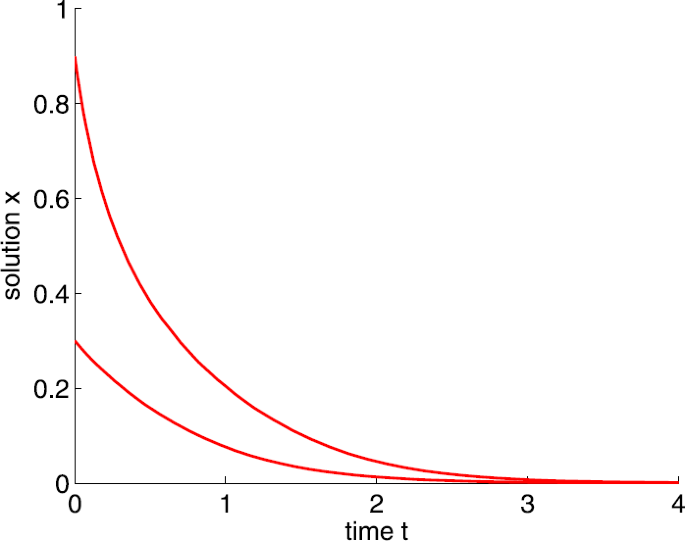
Dynamic behaviors of system (1) with \(A=0.5\), \(d=2\), \(b=5\), and \(a=6\)
-
(ii)
If \(a=10\), that is, \(a>a_{1}\), further if \(0< x(0)<0.2298\), then \(\lim_{t\to +\infty }x(t)=0\); if \(0.2298< x(0)\), then \(\lim_{t\to +\infty }x(t)=0.8702\) (see Fig. 2).
Figure 2 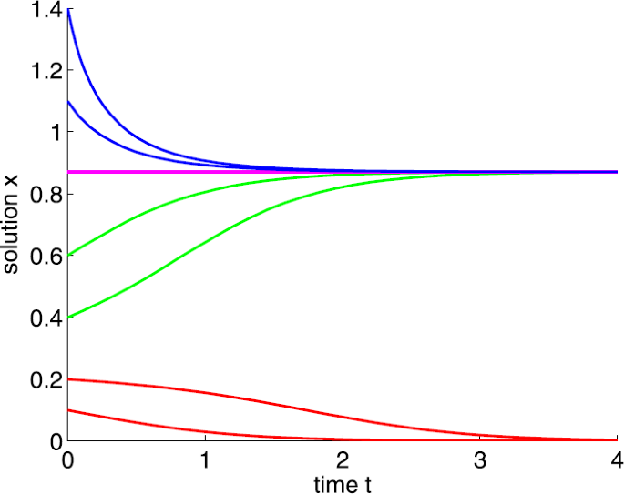
Dynamic behaviors of system (1) with \(A=0.5\), \(d=2\), \(b=5\), and \(a=10\)


In the following, we give the positivity and boundedness of a solution of system (4).
Lemma 2.2
Every solution of system (4) with the initial condition (5) is positive and ultimately bounded for all \(t\geq 0\).
Proof
It can be easily proved that every solution of system (4) with (5) remains positive for all \(t\geq 0\). Let \(V(t)=nx(t)+y(t-\tau )\), calculating the derivative of \(V(t)\) with respect to t along the positive solution of system (4), we then have
By Theorem 2.1, there exist some positive constants B and T such that \(\dot{V}(t) \leq B-{\delta }V(t)\) for all \(t \geq T\). Thus \(\overline{\lim_{t\to +\infty }}V(t) \leq \frac{\delta }{B}\); consequently, \(x(t)\) and \(y(t)\) are ultimately bounded. The proof is complete. □
Let \(\dot{x}=\dot{y}=0\) in system (4), then
There always exists a trivial equilibrium \(E_{0}(0,0)\).
If \(a>a_{1}\), then system (4) has two boundary equilibria \(E_{1}(x_{1},0)\) and \(E_{2}(x_{2},0)\), where
with \(k=a- ( Ab+d )\), \(Q_{1} = a^{2}-2 ( Ab+d ) a+ ( Ab-d ) ^{2}\).
Further, if
then system (4) has a positive equilibrium
where
Obviously,
where \(a_{2}=a_{1}\) if and only if \(A= \frac{b(x^{*})^{2}}{d}\).
The above analysis can be summarized in Table 1.
Define
If \(a\leq d\), it follows from Table 1 that there exists only one trivial equilibrium \(E_{0}\) of system (4) for all A. Hence, in the following, we only consider \(a>d\). When \(Q_{0}\leq 0\), there does not exist a positive equilibrium \(E^{*}\) of system (4), so we assume that \(Q_{0}>0\), that is, \(x^{*}>0\). Note that \(a>a_{1}\) is equivalent to \(a>d\) and \(A< A_{1}\), and \(a>a_{2}\) is equivalent to \(a>d\) and \(A< A_{2}\). When \(x^{*}\geq \frac{a-d}{b}\), \(A_{2}\leq 0\), which means that system (4) does not admit a positive equilibrium \(E^{*}\). Note that \(A_{1}>0\). Hence, to ensure \(A_{2}>0\), we must assume that \(0< x^{*}< \frac{a-d}{b}\). By simple computation, we have
particularly \(A_{1}=A_{2}\) if and only if \(x^{*}=x_{0}^{*}\). We summarize the above results in Table 2.
Tables 1 and 2 show that if the birth rate a is relatively small or the Allee effect A is relatively large, then system (4) only has one trivial equilibrium \(E_{0}\), that is, the predator and prey will be extinct. If the birth rate a is relatively large or the Allee effect A is relatively small, then system (4) has a positive equilibrium \(E^{*}\), which guarantees the coexistence of system (4).
3 Local stability and Hopf bifurcation
3.1 \(E_{0}=(0,0)\)
Firstly, we discuss the stability of \(E_{0}\). We obtain the following theorems.
Theorem 3.1
\(E_{0}\) of system (4) is locally asymptotically stable.
Proof
The variational matrix of system (4) at \(E_{0}\) is
Clearly, the characteristic equation of the equilibrium point \(E_{0}\) always has two negative real roots: \(\lambda _{1} = -d\), \(\lambda _{2} = -\delta \). The proof is complete. □
Therefore, \(E_{0}\) is always a locally stable node, which implies that both predators and prey will become extinct when their population densities lie in the attraction region of \(E_{0}\). In particular, if the population density of prey becomes low, then both prey and predators will become extinct.
According to Theorem 2.1 and the comparison theorem, it is easy to prove the following theorem.
Theorem 3.2
Assume that \(a < a_{1}\), then \(E_{0}\) of system (4) is globally asymptotically stable.
Remark 3.1
When \(a\leq d\), it follows from Theorem 3.2 that \(E_{0}\) of system (4) is globally asymptotically stable for any value of the Allee effect. It is easy to show that the condition \(a< a_{1}\) of Theorem 3.2 is equivalent to \(a>d\) and \(A> A_{1}\), which implies that both prey and predators will go extinct if the Allee effect is strong. Also, we can see that the Allee effect of prey species increases the extinction risk of both predators and prey. Only when the Allee effect is small, the species may not be extinct.
3.2 \(E_{1}=(x_{1},0)\)
We study the local stability of the boundary equilibrium \(E_{1}(x_{1},0)\) and have the following theorem.
Theorem 3.3
-
(1)
Assume that \(Q_{0}>0\) and \(A<\frac{b(x^{*})^{2}}{d}\) hold.
-
(2)
Assume that \(Q_{0}>0\) and \(A \geq \frac{b(x^{*})^{2}}{d}\) hold. If \(a>a_{1}\), then \(E_{1}\) of system (4) is unstable.
-
(3)
Assume that \(Q_{0}\leq 0\) holds. If \(a>a_{1}\), then \(E_{1}\) of system (4) is locally asymptotically stable.
Proof
The variational matrix of system (4) at the equilibrium point \(E_{1}\) is
and its associated characteristic equation is
First, we consider the following equation:
Then we obtain
Obviously, \(( a-d ) Q_{1} > 0\). Further, we consider an equation in a as follows:
Since
and the symmetry axis of \(f_{1}(a)\) is \(\overline{a} = \frac{Ab}{2}+d < a_{1}\), the inequality \(f_{1}(a) > 0\) holds for all \(a > a_{1}\). Therefore, we have \({\lambda _{1}} < 0\), then Eq. (15) has only one negative real root, which implies that all other roots of Eq. (14) are determined by the following equation:
Denote \(\mathfrak{R}_{0} = \frac{N}{\delta }\), \(N=\frac{knm+nm\sqrt{Q_{1}}}{2b+hk+h\sqrt{Q_{1}}}\), and \(a^{0}_{1}=Ab+d+2bx^{*}\). We have the following discussion.
-
(i)
Assume that \(\mathfrak{R}_{0} > 1\), that is, \(\delta < N\), then \(F_{2}(0) < 0\) and \(F_{2}(+\infty ) = +\infty \). Hence \(F_{2}(\lambda )\) has at least one positive root and \(E_{1}\) is unstable.
-
(ii)
If \(\mathfrak{R}_{0} <1\), then \(N<\delta \). Suppose that there exists an eigenvalue λ with \(\operatorname{Re} \lambda \geq 0\), then we have
$$\begin{aligned} \operatorname{Re}\lambda &= N{e^{-\operatorname{Re}(\lambda ){\tau }}}\cos (\operatorname{Im}\lambda ){ \tau }-\delta \\ & \leq N{e^{-\operatorname{Re}(\lambda ){\tau }}}-N < 0. \end{aligned}$$(19)It is a contradiction, so \(\operatorname{Re}\lambda < 0\). This implies that all the real parts of roots of \(F_{2}(\lambda ) =0\) are negative. Hence \(E_{1}\) is a locally asymptotically stable equilibrium.
On the one hand, when \(Q_{0}>0\), we know \(a_{1}=a^{0}_{1}=a_{2}\) if and only if \(A=\frac{b(x^{*})^{2}}{d}\). Thus \(a^{0}_{1}< a_{1}< a_{2}\) if \(A>\frac{b(x^{*})^{2}}{d}\); if \(A<\frac{b(x^{*})^{2}}{d}\), then \(a_{1}< a_{2}< a^{0}_{1}\). By calculation, for any \(a>a_{1}\), we have
where \(H(a)=a-a^{0}_{1}+\sqrt{a^{2}-2(Ab+d)a+(Ab-d)^{2}}\).
Hence, we obtain the following conclusions:
-
(1)
Assume that \(A<\frac{b(x^{*})^{2}}{d}\), that is, \(a_{1}< a_{2}< a^{0}_{1}\), then:
-
(i)
Let \(a_{1}< a< a^{0}_{1}\). When \(a_{1}< a< a_{2}\), we have \(H(a)<0\), that is, \(\mathfrak{R}_{0}<1\). Thus \(E_{1}\) of system (4) is locally asymptotically stable; if \(a_{2}< a< a^{0}_{1}\), then \(H(a)>0\), that is, \(\mathfrak{R}_{0}>1\), which means \(E_{1}\) of system (4) is unstable.
-
(ii)
If \(a^{0}_{1} \leq a\), then \(H(a)>0\), that is, \(\mathfrak{R}_{0}>1\). Therefore, \(E_{1}\) of system (4) is unstable.
-
(i)
-
(2)
If \(A \geq \frac{b(x^{*})^{2}}{d}\), then \(a_{1}\geq a^{0}_{1}\). Therefore, we have \(H(a)>0\) for any \(a>a_{1}\), that is, \(\mathfrak{R}_{0}>1\). Hence \(E_{1}\) of system (4) is unstable.
On the other hand, when \(Q_{0}\leq 0\), it follows from (20) that
that is, \(\mathfrak{R}_{0}<1\). Hence, if \(a>a_{1}\), then \(E_{1}\) of system (4) is locally asymptotically stable.
Summarizing the above discussion, we prove Theorem 3.3. □
3.3 \(E_{2}=(x_{2},0)\)
Theorem 3.4
Let \(a>a_{1}\), then \(E_{2}\) of system (4) is unstable.
Proof
The variational matrix of system (4) at the equilibrium point \(E_{2}\) is
and its associated characteristic equation is
We consider the following equation:
Then we obtain
where
Let \(\sqrt{Q_{1}} =t\), then \(t>0\). Hence, Eq. (24) can be rewritten as
Solving the equation \(g(t)=0\), we can get
where \(f_{1}(a)\) is defined by (17). Similar to the analysis of Theorem 3.3, we obtain \(f_{1}(a) >0\), thus \(t_{2} =f_{1}(a)/(a-d) >0\).
Hence, if \(0 < t < t_{2}\), then \(g(t) < 0\); if \(t_{2} \leq t\), then \(g(t) \geq 0\). That is, if \(0 < Q_{1} < t_{2}^{2}\), then \(G_{2}(Q_{1}) < 0\); if \(t_{2}^{2} \leq Q_{1}\), then \(G_{2}(Q_{1}) \geq 0\). Clearly, the inequality \(t_{2}^{2} \leq Q_{1}\) does not hold, due to \(Q_{1}-t_{2}^{2} =-\frac{4A^{2}b^{2}ad}{(a-d)^{2}} <0\), which is a contradiction. Thus \(\lambda >0\), which implies Eq. (21) has at least one positive root and \(E_{2}\) is unstable. The proof of the theorem is complete. □
We summarize the results of Theorems 3.3 and 3.4 in Table 3. On the other hand, by the analysis of Sect. 2 and Theorems 3.3 and 3.4, we also obtain the local asymptotic stability of equilibria \(E_{i}, i=0,1,2\) (see Table 4).
By the definition of \(\mathfrak{R}_{0}\) and simple computation, from the proofs of Theorems 3.3 and 3.4, we can obtain the following corollaries.
Corollary 3.1
Let \(a>d\) and \(0< A< A_{1}\), then \(E_{1}\) of system (4) is:
-
(i)
unstable if \(0< h< \frac{nm}{\delta }-\frac{1}{x_{1}}\),
-
(ii)
locally asymptotically stable if \(h> \frac{nm}{\delta }-\frac{1}{x_{1}}\).
Corollary 3.2
Let \(a>d\) and \(0< A< A_{1}\), then \(E_{2}\) of system (4) is unstable.
When \(\tau =0\), by computation, the conditions of Corollaries 3.1 and 3.2 are the same as those of Theorems 1 and 2 [29]. Hence, we extend the local asymptotic stability results for system (3) to the time delay system (4). It shows that both \(E_{1}\) and \(E_{2}\) of system (4) are still locally asymptotically stable under the same condition as those for the nondelay system (3). Therefore, the time delay is harmless for the local stability of \(E_{1}\) and \(E_{2}\). Also, when considering the birth rate a or the Allee effect A as a parameter, we get the threshold condition for the stability of \(E_{0}, i=0,1,2\), of system (4). Hence, we obtain some more precise conditions than those of [29].
3.4 \(E^{*}=(x^{*},y^{*})\)
The variational matrix of system (4) at \(E^{*}\) is
Now, to determine the local stability of the interior equilibrium \(E^{*}\), we use the method introduced by Beretta and Kuang [38]. Then the characteristic equation at \(E^{*}\) is
where
For the interior equilibrium \(E^{*}\), we have
When \(\tau = 0\), Eq. (27) reduces to
From (28), we can obtain
Next, we consider \(p_{1}+q_{1}\). Using Eq. (28), we have
where
Define
then
Note that
Let \(A<\frac{b(x^{*})^{2}}{d}\), then \(a_{3}>a_{2}\). If \(a< a_{3}\), then \(p_{1}+q_{1}=B_{1}(a_{3}-a)>0\); if \(a>a_{3}\), then \(p_{1}+q_{1}<0\). If \(A \geq \frac{b(x^{*})^{2}}{d}\) and \(a>a_{2}\), then \(p_{1}+q_{1}<0\). Accordingly, by the Routh–Hurwitz criterion, if \(p_{0}+q_{0}>0\) and \(p_{1}+q_{1}>0\), then \(E^{*}\) is locally asymptotically stable when \(\tau =0\). We have the following theorem.
Theorem 3.5
Let \(\tau =0\) and \(Q_{0}>0\) hold.
-
(1)
Assume that \(A<\frac{b(x^{*})^{2}}{d}\) holds.
-
(2)
If \(A \geq \frac{b(x^{*})^{2}}{d}\) and \(a>a_{2}\), then \(E^{*}\) of system (4) is unstable.
Next, under the conditions \(Q_{0}>0\) and \(A<\frac{b(x^{*})^{2}}{d}\), we discuss system (4) with \(\tau >0\). Then, we discuss (27) has a pair of purely imaginary roots. iω (\(\omega >0\)) is a solution of (27) if and only if ω satisfies
that is,
which implies
By calculation, we derive that
and from (30) we have
Further, we consider \(p_{0}-q_{0}\). From (28) we have
where
On the other hand, we denote
Then we have
Note that, due to \(A<\frac{b(x^{*})^{2}}{d}\), we derive that
and
By Theorem 3.5, if \(a_{2}< a\leq a_{4}\), \(p_{0}-q_{0}\geq 0\); if \(a_{4}< a< a_{3}\), \(p_{0}-q_{0}<0\).
When \(p_{0}-q_{0} < 0\), \(\omega _{0}\) is a unique positive root of Eq. (33), that is, Eq. (27) has the roots of the form \(\pm i\omega _{0}\), where
From (32), we obtain
Denote
By Theorem 3.4.1 in Kuang [39], if \(p_{0}< q_{0}\), then \(E^{*}\) is still stable for \(\tau <\tau _{0} :=\tau _{00}\).
Taking the derivative of Eq. (27) with respect to τ, one has
Hence, a direct calculation shows that
We derive from (32) that
which yields
When \(\omega =\omega _{0}\), \(\tau =\tau _{0}\), a Hopf bifurcation occurs.
The above analysis can be summarized in the following theorem.
Theorem 3.6
Let \(Q_{0}>0\) and \(A<\frac{b(x^{*})^{2}}{d}\) hold.
-
(i)
If \(a_{2} < a \leq a_{4} \), then \(E^{*}\) of system (4) is locally asymptotically stable for all \(\tau \geq 0\).
-
(ii)
If \(a_{4} < a < a_{3}\) holds, then \(E^{*}\) is a locally asymptotically stable equilibrium if \(0< \tau <\tau _{0}\) and unstable if \(\tau > \tau _{0}\).
Further, system (4) undergoes a Hopf bifurcation at \(E^{*}\) when \(\tau =\tau _{0}\).
4 Numeric simulations
We present some examples to verify our results.
Example 4.1
In system (4), assume that \(A=0.5\), \(d=1\), \(b=5\), \(m=5\), \(n=1\), \(h=0.1\), \(\tau =1\), and \(\delta =6\), then \(a_{1}=6.6623\).
-
(i)
If \(a=5\), that is, \(a< a_{1}\), it follows from Theorem 3.2 that \(E_{0}\) is globally asymptotically stable. Hence, both prey and predators are extinct (see Fig. 3).
Figure 3 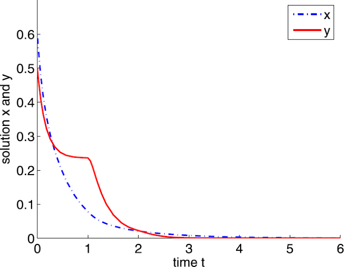
Dynamic behaviors of system (4) with \(A=0.5\), \(d=1\), \(b=5\), \(m=5\), \(n=1\), \(h=0.1\), \(\tau =1\), \(\delta =6\), and \(a=5\)
-
(ii)
If \(a=8\), then system (4) has a boundary equilibrium \(E_{1}=(0.7702,0)\). Note that \(A=0.5<9.2975=\frac{b(x^{*})^{2}}{d}\), \(a_{1}< a<10.6848=a_{2}\). By Theorem 3.3, \(E_{1}\) is locally asymptotically stable (see Fig. 4).
Figure 4 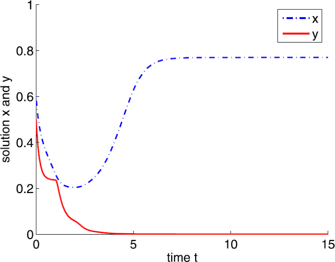
Dynamic behaviors of system (4) with \(A=0.5\), \(d=1\), \(b=5\), \(m=5\), \(n=1\), \(h=0.1\), \(\tau =1\), \(\delta =6\), and \(a=8\)


Example 4.2
In system (4), assume that \(A=0.5\), \(d=1\), \(b=5\), \(m=5\), \(n=1\), \(h=0.1\), \(\delta =6\), and \(\tau =0\). By calculation, we have \(Q_{0}=4.4>0\), \(A<\frac{b(x^{*})^{2}}{d}=9.2975\), \(a_{2}=10.6848\), and \(a_{3}=27.2999\).
-
(i)
If \(a=15\), it is easy to show that \(a_{2}< a< a_{3}\). We can obtain a positive equilibrium \(E^{*}=(1.3636,0.7176)\). By Theorem 3.5, \(E^{*}\) is locally asymptotically stable (see Fig. 5).
Figure 5 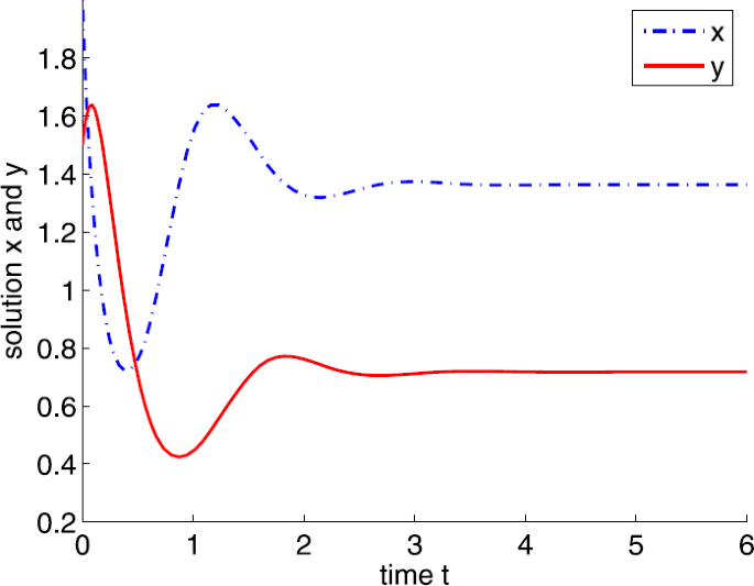
Dynamic behaviors of system (4) with \(A=0.5\), \(d=1\), \(b=5\), \(m=5\), \(n=1\), \(h=0.1\), \(\delta =6\), \(\tau =0\), and \(a=15\)
-
(ii)
If \(a=30\), then \(a>a_{3}\). Also, we can obtain a positive equilibrium \(E^{*}=(1.3636,3.2121)\). By Theorem 3.5, \(E^{*}\) is unstable (see Fig. 6).
Figure 6 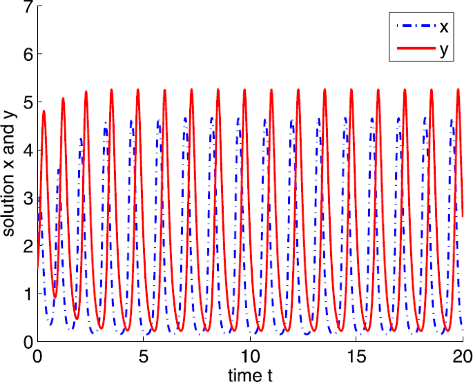
Dynamic behaviors of system (4) with \(A=0.5\), \(d=1\), \(b=5\), \(m=5\), \(n=1\), \(h=0.1\), \(\delta =6\), \(\tau =0\), and \(a=30\)


Example 4.3
In system (4), let \(a=4\), \(A=0.02\), \(d=2\), \(b=1\), \(m=n=4\), \(h=0.1\), \(\delta =3\). By calculation, we have \(Q_{0}=15.7>0\), \(A=0.02>0.0183=\frac{b(x^{*})^{2}}{d}\), \(a>a_{2}=2.4204\), and there is a positive equilibrium \(E^{*}=(0.1911,0.4102)\). By Theorem 3.5, \(E^{*}\) is unstable, that is, both the predator and prey species will be extinct (see Fig. 7).

Dynamic behaviors of system (4) with \(a=4\), \(A=0.02\), \(d=2\), \(b=1\), \(m=n=4\), \(h=0.1\), \(\delta =3\), and \(\tau =0\)
Example 4.4
In system (4), assume that \(A=0.5\), \(d=1\), \(b=m=5\), \(n=1\), \(h=0.1\), \(\delta =6\). By calculation, we have \(a_{2}=10.6848\), \(a_{3}=27.2999\), \(a_{4}=18.4738\), \(Q_{0} = 4.400>0\), \(x^{*}=1.3636\), and \(A<\frac{b(x^{*})^{2}}{d}=9.2975\).
-
(i)
If \(a=15\) and \(\tau =3\). It is easy to show that \(a_{2}< a< a_{4}\) and the positive equilibrium is \(E^{*}=(1.3636,0.7176)\). By Theorem 3.6, \(E^{*}\) is locally asymptotically stable (see Fig. 8).
Figure 8 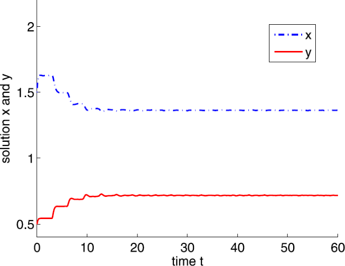
Dynamic behaviors of system (4) with \(a=15\), \(A=0.5\), \(d=1\), \(b=m=5\), \(n=1\), \(h=0.1\), \(\delta =6\), and \(\tau =3\)
-
(ii)
If \(a=15\) and \(\tau =15\). It is easy to show that \(a_{2}< a< a_{4}\) and the positive equilibrium is \(E^{*}=(1.3636,0.7176)\). By Theorem 3.6, \(E^{*}\) is locally asymptotically stable (see Fig. 9).
Figure 9 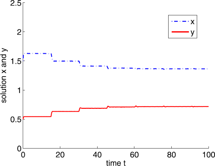
Dynamic behaviors of system (4) with \(a=15\), \(A=0.5\), \(d=1\), \(b=m=5\), \(n=1\), \(h=0.1\), \(\delta =6\), and \(\tau =15\)
-
(iii)
If \(a=20\), clearly, \(a_{4}< a< a_{3}\) and the positive equilibrium is \(E^{*}=(1.3636,1.5491)\). By calculation, we obtain \(\tau _{0}=0.1387\). According to Theorem 3.6, \(E^{*}\) is locally asymptotically stable if \(0<\tau <\tau _{0}\) and unstable if \(\tau >\tau _{0}\), and system (4) undergoes a Hopf bifurcation at \(E^{*}\) when \(\tau =\tau _{0}\), where \(\tau =0.07\) is shown in Fig. 10 and \(\tau =0.15\) is shown in Fig. 11.
Figure 10 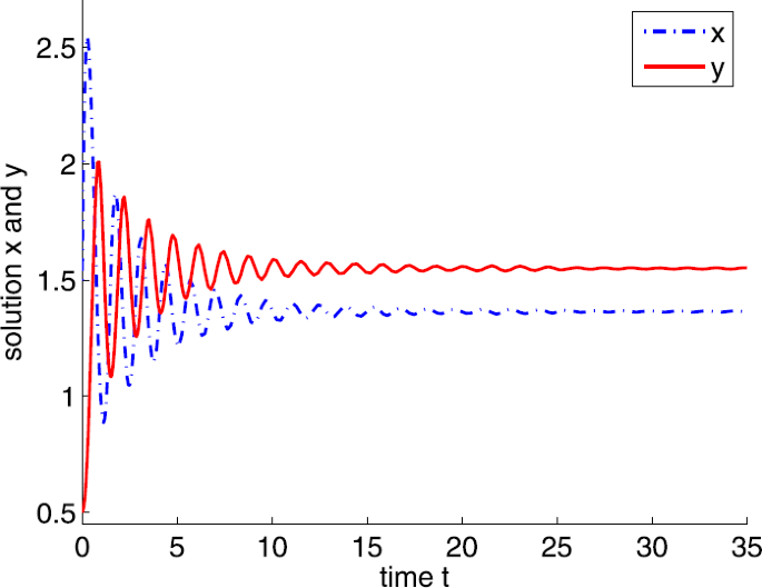
Dynamic behaviors of system (4) with \(a=20\), \(A=0.5\), \(d=1\), \(b=m=5\), \(n=1\), \(h=0.1\), \(\delta =6\), and \(\tau =0.07\)
Figure 11 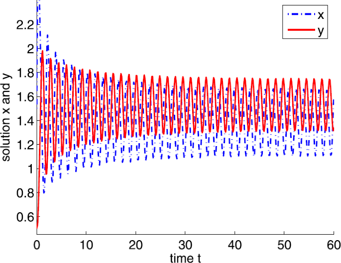
Dynamic behaviors of system (4) with \(a=20\), \(A=0.5\), \(d=1\), \(b=m=5\), \(n=1\), \(h=0.1\), \(\delta =6\), and \(\tau =0.15\)


5 Conclusion
In this paper, we investigate the stability and Hopf bifurcation of a delayed Holling type II predator–prey model when the prey is subject to Allee effect. Considering the birth rate a or the Allee effect A as a parameter, we get the threshold condition for the stability of the equilibria of system (4) and find that the Allee effect or the birth rate plays an important role in the stability of system (4).
Firstly, we analyze the logistic equation (1) with Allee effect, and show that the Allee effect may lead to the instability of the system. By analyzing the characteristic equations, we derive the local stability of the equilibria. Table 3 shows that \(E_{2}\) is always unstable if it exists. If the Allee effect is relatively small, with the increase of the birth rate a, the equilibrium \(E_{1}\) changes from the nonexistence to the local asymptotic stability, and eventually becomes instability. Table 4 shows that the equilibrium \(E_{1}\) changes from instability to local asymptotic stability, and eventually disappears with the increase of Allee effect.
We also investigate the local asymptotic stability of the coexistence equilibrium \(E^{*}\) and show that if the time delay passes through some critical values, the equilibrium \(E^{*}\) changes from a stable point to unstable point, and a Hopf bifurcation occurs; further we show periodic solutions.
Let \(\tau =0\), then system (4) is reduced to system (3). If system (3) has only three equilibrium points \(E_{i}, i=0,1,2\). \(E_{0}(0,0)\) is locally asymptotically stable. Further if \(E_{1}\) and \(E_{2}\) are unstable, then the trivial equilibrium \(E_{0}(0,0)\) is globally asymptotically stable. When system (3) has equilibrium points \(E_{i}, i=0,1,2\), and \(E^{*}\). If \(E_{1}\), \(E_{2}\), and \(E^{*}\) are unstable, then system (3) admits a limit cycle or \(E_{0}(0,0)\) is globally asymptotically stable. In Table 5, compared with Zu and Mimura [29], we give the threshold condition for the stability of \(E_{0}, i=0,1,2\), and \(E^{*}\) of system (4) with \(\tau =0\). Therefore, our main results complement and improve those in [29].
In Theorem 3.6, we study the stability and Hopf bifurcation of system (4). The results of Theorems 3.1–3.6 are shown in Table 6. If the Allee effect is small, the equilibrium \(E_{1}\) changes from the nonexistence to the local asymptotic stability, and eventually becomes instability with the increase of the birth rate a. On the other hand, the equilibrium \(E^{*}\) changes from the nonexistence to the local asymptotic stability, and eventually a Hopf bifurcation occurs with the increase of the birth rate a. When the initial densities of prey and predators are not low, we show the results of Table 6 in Fig. 12 and Fig. 13 with the same initial values. Change the values of the birth rate a from zero to \(a_{1}\), the prey species will stabilize at zero, from \(a_{1}\) to \(a_{2}\), the prey species will stabilize at \(x_{1}\). From \(a_{2}\) to \(a_{3}\), the prey species will stabilize at \(x^{*}\). Finally, the prey species becomes oscillation if \(a_{4}< a< a_{3}\). The predator species has the similar case. Hence, we find that both the predator species and the prey species go to extinction when the prey population has a sufficiently small birth rate a. As a increases, the prey species could survive, but the predator is still extinct. Keeping the birth rate a increasing, the prey and the predator will coexist and stabilize at a fixed value. But if it is large enough, the stability of prey and predators will be destroyed, and the system becomes oscillation. Hence, in this paper, we show that we can choose a suitable value of the Allee effect or the birth rate to influence the stability of system (4).

Dynamic behaviors of the prey in system (4) with \(A=0.5\), \(d=1\), \(b=m=5\), \(n=1\), \(h=0.1\), \(\delta =6\), \(\tau =0.5\), and \(a=4\) or 8 or 15 or 20

Dynamic behaviors of the predator in system (4) with \(A=0.5\), \(d=1\), \(b=m=5\), \(n=1\), \(h=0.1\), \(\delta =6\), \(\tau =0.5\), and \(a=4\) or 8 or 15 or 20
References
Shi, C.L., Chen, X.Y., Wang, Y.Q.: Feedback control effect on the Lotka–Volterra prey–predator system with discrete delays. Adv. Differ. Equ. 2017, Article ID 373 (2017)
Chen, F.D., Ma, Z.Z., Zhang, H.Y.: Global asymptotical stability of the positive equilibrium of the Lotka–Volterra prey–predator model incorporating a constant number of prey refuges. Nonlinear Anal., Real World Appl. 13(6), 2790–2793 (2012)
Ma, Z.Z., Chen, F.D., Wu, C.Q., Chen, W.L.: Dynamic behaviors of a Lotka–Volterra predator–prey model incorporating a prey refuge and predator mutual interference. Appl. Math. Comput. 219(15), 7945–7953 (2013)
Chen, F.D., Chen, W.L., Wu, Y.M., Ma, Z.Z.: Permanence of a stage-structured predator–prey system. Appl. Math. Comput. 219(17), 8856–8862 (2013)
Chen, L.J., Chen, F.D.: Dynamic behaviors of the periodic predator–prey system with distributed time delays and impulsive effect. Nonlinear Anal., Real World Appl. 12(4), 2467–2473 (2011)
Chen, F.D., Xie, X.D., Miao, Z.S., Pu, L.Q.: Extinction in two species nonautonomous nonlinear competitive system. Appl. Math. Comput. 274, 119–124 (2016)
Holling, C.S.: The functional response of predator to prey density and its role in mimicry and population regulation. Can. Entomol., Suppl. 97(S45), 5–60 (1965)
Xu, R.: Global stability and Hopf bifurcation of a predator–prey model with stage structure and delayed predator response. Nonlinear Dyn. 67(2), 1683–1693 (2012)
Aziz-Alaoui, M.A., Okiye, M.D.: Boundedness and global stability for a predator–prey model with modified Leslie–Gower and Holling-type II schemes. Appl. Math. Lett. 16(7), 1069–1075 (2003)
Lin, Q.X., Xie, X.D., Chen, F.D., Lin, Q.F.: Dynamical analysis of a logistic model with impulsive Holling type-II harvesting. Adv. Differ. Equ. 2018, Article ID 112 (2018)
Chen, L.J., Chen, F.D., Chen, L.J.: Qualitative analysis of a predator–prey model with Holling type II functional response incorporating a constant prey refuge. Nonlinear Anal., Real World Appl. 11(1), 246–252 (2010)
Allee, W.C.: Animal Aggregations: A Study in General Sociology. University of Chicago Press, Chicago (1932)
Kuussaari, M., Saccheri, I., Camara, M., Hanski, I.: Allee effect and population dynamics in the Glanville fritillary butterfly. Oikos 82, 384–392 (1998)
Stephens, P.A., Sutherland, W.J.: Consequences of the Allee effect for behaviour, ecology and conservation. Trends Ecol. Evol. 14(10), 401–405 (1999)
Courchamp, F., Grenfell, B., Clutton-Brock, T.: Population dynamics of obligate cooperators. Proc. R. Soc. Lond. B 266(1419), 557–563 (1999)
Liu, X.S., Dai, B.X.: Dynamics of a predator–prey model with double Allee effects and impulse. Nonlinear Dyn. 88(1), 685–701 (2017)
Biswas, S., Sasmal, S.K., Samanta, S., Saifuddin, M., Pal, N., Chattopadhyay, J.: Optimal harvesting and complex dynamics in a delayed eco-epidemiological model with weak Allee effects. Nonlinear Dyn. 87(3), 1553–1573 (2017)
Manna, D., Maiti, A., Samanta, G.P.: A Michaelis-Menten type food chain model with strong Allee effect on the prey. Appl. Math. Comput. 311, 390–409 (2017)
Zu, J., Mimura, M., Wakano, J.Y.: The evolution of phenotypic traits in a predator–prey system subject to Allee effect. J. Theor. Biol. 262(3), 528–543 (2010)
González-Olivares, E., Rojas-Palma, A.: Multiple limit cycles in a Gause type predator–prey model with Holling type III functional response and Allee effect on prey. Bull. Math. Biol. 73(6), 1378–1397 (2011)
Guan, X.Y., Liu, Y., Xie, X.D.: Stability analysis of a Lotka–Volterra type predator–prey system with Allee effect on the predator species. Commun. Math. Biol. Neurosci. 2018, Article ID 9 (2018)
Wu, R.X., Li, L., Lin, Q.F.: A Holling type commensal symbiosis model involving Allee effect. Commun. Math. Biol. Neurosci. 2018, Article ID 6 (2018)
Lin, Q.F.: Allee effect increasing the final density of the species subject to the Allee effect in a Lotka–Volterra commensal symbiosis model. Adv. Differ. Equ. 2018, Article ID 196 (2018).
Lin, Q.F.: Stability analysis of a single species logistic model with Allee effect and feedback control. Adv. Differ. Equ. 2018, Article ID 190 (2018)
Chen, B.G.: Dynamic behaviors of a commensal symbiosis model involving Allee effect and one party can not survive independently. Adv. Differ. Equ. 2018, Article ID 212 (2018)
Pal, P.J., Saha, T., Sen, M., Banerjee, M.: A delayed predator–prey model with strong Allee effect in prey population growth. Nonlinear Dyn. 68(1–2), 23–42 (2012)
Ferdy, J.B., Molofsky, J.: Allee effect, spatial structure and species coexistence. J. Theor. Biol. 217(4), 413–424 (2002)
Zu, J.: Global qualitative analysis of a predator–prey system with Allee effect on the prey species. Math. Comput. Simul. 94, 33–54 (2013)
Zu, J., Mimura, M.: The impact of Allee effect on a predator–prey system with Holling type II functional response. Appl. Math. Comput. 217(7), 3542–3556 (2010)
Li, Z., He, M.X.: Hopf bifurcation in a delayed food-limited model with feedback control. Nonlinear Dyn. 76(2), 1215–1224 (2014)
Li, Z., Han, M.A., Chen, F.D.: Global stability of a predator–prey system with stage structure and mutual interference. Discrete Contin. Dyn. Syst., Ser. B 19(1), 173–187 (2014)
Yang, K., Miao, Z.S., Chen, F.D., Xie, X.D.: Influence of single feedback control variable on an autonomous Holling-II type cooperative system. J. Math. Anal. Appl. 435(1), 874–888 (2016)
Chen, Y.M., Zhang, F.Q.: Dynamics of a delayed predator–prey model with predator migration. Appl. Math. Model. 37(3), 1400–1412 (2013)
Yuan, S.L., Ji, X.H., Zhu, H.P.: Asymptotic behavior of a delayed stochastic logistic model with impulsive perturbations. Math. Biosci. Eng. 14(5–6), 1477–1498 (2017)
Song, Y.L., Yin, T., Shu, H.Y.: Dynamics of a ratio-dependent stage-structured predator–prey model with delay. Math. Methods Appl. Sci. 40(18), 6451–6467 (2017)
Chen, L.J., Chen, F.D.: Global stability and bifurcation of a ratio-dependent predator–prey model with prey refuge. Acta Math. Sinica (Chin. Ser.) 57(2), 301–310 (2014)
Wang, Y.Q., Chen, L.J., Gao, H.Y.: Global analysis of a ratio-dependent predator–prey system incorporating a prey refuge. J. Nonlinear Funct. Anal. 2017, 1–26 (2017)
Beretta, E., Kuang, Y.: Geometric stability switch criteria in delay differential systems with delay dependent parameters. SIAM J. Math. Anal. 33(5), 1144–1165 (2002)
Kuang, Y.: Delay Differential Equations with Applications in Population Dynamics. Academic Press, New York (1993)
Acknowledgements
The authors would like to thank Dr. Xinyu Guan for useful discussion about the mathematical modeling.
Funding
The research was supported by the National Natural Science Foundation of China under Grant (11601085) and the Natural Science Foundation of Fujian Province (2017J01400).
Author information
Authors and Affiliations
Contributions
All authors contributed equally to the writing of this paper. All authors read and approved the final manuscript.
Corresponding author
Ethics declarations
Competing interests
The authors declare that there is no conflict of interests.
Additional information
Publisher’s Note
Springer Nature remains neutral with regard to jurisdictional claims in published maps and institutional affiliations.
Rights and permissions
Open Access This article is distributed under the terms of the Creative Commons Attribution 4.0 International License (http://creativecommons.org/licenses/by/4.0/), which permits unrestricted use, distribution, and reproduction in any medium, provided you give appropriate credit to the original author(s) and the source, provide a link to the Creative Commons license, and indicate if changes were made.
About this article

Cite this article
Xiao, Z., Xie, X. & Xue, Y. Stability and bifurcation in a Holling type II predator–prey model with Allee effect and time delay. Adv Differ Equ 2018, 288 (2018). https://doi.org/10.1186/s13662-018-1742-4
Received:
Accepted:
Published:
DOI: https://doi.org/10.1186/s13662-018-1742-4