
Abstract
Hyperelastic-based plastic constitutive equation based on the multiplicative decomposition of the deformation gradient tensor is reviewed comprehensively and its exact formulation is given for the description of the finite deformation and rotation in this article. Further, it is extended to describe the general loading behavior including the monotonic, the cyclic and the non-proportional loading behaviors by incorporating the rigorous plastic flow rules and the subloading surface model. In addition, it is extended also to the rate-dependency based on the overstress model, and the exact hyperelastic-based plastic constitutive equation of friction is formulated by incorporating the subloading-friction model. They are the exact constitutive equations describing the monotonic and the cyclic loading behavior up to the finite deformation/rotation and the friction behavior under the finite sliding/rotation with the rate-dependency, which have remained to be unsolved for a long time, although they have been required in the history of elastoplasticity theory.
1 Introduction
The elastic deformation and the plastic deformation are physically different to each other such that the former is induced by the deformation of material particles themselves but the latter is induced by the mutual slips between the material particles. Therefore, the elastoplasticity is based on the premise that the deformation is decomposed into the elastic and the plastic deformations, so that the irreversible change of substructure is described by the isotropic and the anisotropic hardenings which evolve only by the plastic deformation, while the elastic deformation is irrelevant to the irreversible change of substructure. Here, it should be noticed that the deformation and its rate can be described exactly by the deformation gradient tensor which transforms the reference infinitesimal line element to the current one. Therefore, the exact elastoplastic constitutive equation must be formulated by incorporating the definite decomposition of the deformation gradient tensor into the elastic and the plastic parts which is realized by the multiplicative decomposition of the deformation gradient tensor [52, 55, 56, 58,59,60]. However, it now passed already a half century after the proposition of the multiplicative decomposition of deformation gradient tensor. In the meantime, unfortunately the hypoelastic-based plasticity has been studied enthusiastically by numerous workers represented by Rodney Hill and James R. Rice after the proposition of the hypoelasticity by Truesdell [83], which is not based on the multiplicative decomposition definitely.
The multiplicative hyperelastic-based plasticity has been studied centrally by Simo and his colleagues (e.g. [68, 74,75,76,77, 79,79,80,81]) in the last century, in which the logarithmic strain has been used mainly leading to the co-axiality of stress and strain rate so that it has been limited to the isotropy. It has been developed actively from this century on by Menzel and Steinmann [63], Wallin et al. [87], Dettmer and Reese [14], Menzel et al. [64], Wallin and Ristinmaa [86], Gurtin and Anand [18], Sansour et al. [73], Vladimirov et al. [84, 85], Henann and Anand [47], Hashiguchi and Yamakawa [46], Brepols et al. [6], Hashiguchi [27, 31], etc. in which constitutive relations are formulated in the intermediate configuration imagined fictitiously by the hyperelastic unloading to the stress-free state. However, the plastic flow rule with the generality for the elastically anisotropy remains unsolved and only the conventional plasticity model (named by Drucker [15]) with the yield surface enclosing the elastic domain have been incorporated so that only the monotonic loading behavior of elastically-isotropic materials are concerned in them.
The precise description of the plastic strain rate induced by the rate of stress inside the yield surface is inevitable for the prediction of cyclic loading behavior which is crucial for the accurate mechanical design of solids and structures in engineering. A lot of works have been executed and various unconventional plastic constitutive (cyclic plasticity) models (named by Drucker [15]) have been proposed aiming at describing the plastic strain rate caused by the rate of stress inside the yield surface after 1960s when the demands of mechanical designs for the vibration proof and the earthquake proof have been highly raised responding to the high development of machine industries and the frequent occurrences of earthquakes in Niigata (Japan) and Chili, etc. Among various unconventional models the multi surface model [51, 66], the two surface model [12, 53, 91] and the superposed-kinematic hardening model [10, 67] are well-known. However, they inherit a small yield surface enclosing purely-elastic domain from the conventional plasticity model and are based on the premise that the plastic strain rate develops with the translation of the small yield surface so that they are called the cyclic kinematic hardening model. Therefore, they possess various defects, e.g. (1) the abrupt transition from the elastic to the plastic state violating the continuity and the smoothness conditions [21, 22, 24], (2) the incorporation of the offset value of the plastic strain at yield, (3) the incapability of cyclic loading behavior for the stress amplitude less than the small yield surface assumed inside the conventional yield surface, (4) the incapability of the non-proportional loading behavior, (5) the incapability of extension to the rate-dependency at high rate of deformation up to the impact loading behavior, (6) the limitation to the description of deformation behavior in metals, (7) the necessity of the additional cumbersome operation to pull-back the stress to the yield surface. On the other hand, only the subloading surface model [19, 20, 33] does not incorporate the yield surface enclosing a purely-elastic domain so that it possesses the high ability for describing not only the monotonic but also the cyclic and the non-proportional loading behaviors, resolving all the above-mentioned defects in the other elastoplasticity models. In addition, it possesses the automatic controlling function to pull-back the stress to the yield surface when the stress goes out from the yield surface in numerical calculations [19, 20, 33]. It is capable of describing the elastoplastic deformation behavior in not only metals but also soils [38, 42, 89] and further the friction behavior rigorously [24, 26, 40, 41]. It would be regarded to be the governing law of the irreversible mechanical phenomena of solids.
The subloading surface model has been incorporated to the commercial software Marc 2017.1 version in Marc Software Corporation as the standard installation by the name “Hashiguchi model”, which can be used by all Marc contractors (users). Therefore, it is explained in the Marc user manual [61] in brief. Needless to say, however, it is limited to the formulation in the ordinary current configuration, whereas there is no commercial software installed the multiplicative hyperelastic-based plastic constitutive equation up to date.
First, the basic frameworks of the elastoplastic constitutive equations will be reviewed briefly in order to confirm the necessity of the multiplicative decomposition of the deformation gradient tensor into the elastic and the plastic parts. Therein, the fundamentals in the multiplicative decomposition will be delineated concisely where the interpretation of the isoclinic concept is given thoroughly. Then, the exact hyperelastic-based plastic constitutive equation will be formulated within the framework of the multiplicative decomposition of the deformation gradient tensor, incorporating the rigorous plastic flow rules and the subloading surface model. It will be extended to the rate-dependency based on the overstress model by revising the former formulations of the overstress model so as to be applicable to the general rate ranging from the quasi-static to the impact loading behaviors [31, 33]. Further, the exact hyperelastic-based plastic constitutive equation of friction is formulated rigorously, in which not only the rotation but also the deformation of the contact surface can be incorporated, although the hypoelastic-based plastic constitutive equation has been formulated in the past [31, 33, 40, 41]. They are the exact constitutive equations describing not only the monotonic and the cyclic loading behavior under the finite deformation/rotation and the cyclic friction behavior under the finite sliding/rotation. Then, the comprehensive review will be given for the multiplicative hyperelastic-based plasticity for finite deformation/rotation and finite friction-sliding/rotation, incorporating the various novel, rational formulations which have not been shown in existing literatures.
The direct notations \( {\mathbf{u}} \cdot {\mathbf{v}} \)\( {\text{for}} \)urvr, \( {\mathbf{u}} \otimes {\mathbf{v}} \) for uivj, \( {\mathbf{Av}} \) for Airvr, \( {\mathbf{A}:{\bf B}} \) for ArsBrs, \( {\mathbf{AB}} \) for AirBrj, \( {\boldsymbol{\Gamma}} :{\mathbf{A}} \) for ΓijrsArs, \( {\mathbf{A}}:{\boldsymbol{\Gamma}} \) for ArsΓrsij, \( {\mathbf{A}} \otimes {\mathbf{B}} \) for AijBkl and \( {\boldsymbol{\Gamma}}:{\boldsymbol{\Xi }} \) for ΓijrsΞrskl are used for arbitrary vectors \( {\mathbf{u}} \) and \( {\mathbf{v}} \), second-order tensors \( {\mathbf{A}} \) and \( {\mathbf{B}} \), fourth-order tensors \( {\boldsymbol{\Gamma}} \) and \( {\boldsymbol{\Xi}} \), where the Einstein’s summation convention is applied for letters with repeated indices taking 1, 2, 3. Further, \( {\mathbf{0}} \) and \( {\mathbf{O}} \) stand for the zero vector and tensor, respectively, \( {\mathbf{I}} \) and \( {\varvec{\mathcal{I}}} \) stand for the second-order and the fourth-order identity tensors possessing the components of the Kronecker’s delta δij\( (\delta_{ij} = 1 \, \,\,{\text{for}}\,\, \, i = j ;\,\delta_{ij} = 0 \, \,\,{\text{for}}\,\, \, i \ne j) \) and \( \mathcal{I}_{ijkl} = \delta_{ik} \delta_{jl} \), respectively, \( \text{tr}{\mathbf{A}}= A_{ij} \delta_{ij} \) for the trace, \( {\mathbf{A'}}= {\mathbf{A}} - \text{(tr}{\mathbf{A}}){\mathbf{I}}/3 \) for the deviatoric tensor, \( {\mathbf{A}}^{{ - {1}}} \) for the inverse tensor satisfying \( {\mathbf{AA}}^{{ - {1}}} = {\mathbf{I}} \) and \( \|{\mathbf{A}}\| = \sqrt {A_{ij} A_{ij} } \) for the magnitude and the symbol \( ({ )}^{T} \) for the transposed tensor. The notations \( \text{sym}[{\mathbf{A}}] \equiv ({\mathbf{A}} +{\mathbf{A}}^{T} )/2 \) and \( \text{ant}[{\mathbf{A}}] \equiv ({\mathbf{A}} - {\mathbf{A}}^{T} {)/2} \) stand for the symmetric and the antisymmetric parts, respectively. (·) stands for the material-time derivative. The symbol \( \langle \, \rangle \) designates the Macaulay’s bracket defined by \( \langle s\rangle = (s + |s|/2)\), i.e. \( s < 0: \langle s\rangle = 0 \) and \( s \ge 0: \langle s\rangle = s \) (s: arbitrary scalar variable).
2 Classification of Elastoplastic Constitutive Equations
The advantages of the multiplicative hyperelastic-based plasticity should be clarified prior to its formulation which is to be the purpose of this article. The basic frameworks of elastoplastic constitutive equations are classified and their features are described concisely in the following.
2.1 Infinitesimal Elastoplasticity
-
1.
The infinitesimal strain is additively decomposed into the elastic and the plastic parts.
-
2.
The reference and the current configurations are not distinguished.
-
3.
The Cauchy stress is used as the stress measure.
-
4.
The stress is related to the elastic strain by the hyperelastic relation based on the strain energy potential function.
-
5.
The plastic strain rate is calculated and its accumulation leads to the plastic strain.
-
6.
The elastic strain is calculated by subtracting the plastic strain from the strain.
-
7.
The stress is calculated by substituting the elastic strain into the hyperelastic equation.
-
8.
The infinitesimal elastic and plastic deformation without a rotation is described.
2.2 Hypoelastic-Based Plasticity
-
1.
The symmetric and the anti-symmetric parts of the velocity gradient are defined as the strain rate and the spin, respectively.
-
2.
The strain rate and the spin are additively decomposed into the elastic and the plastic parts.
-
3.
The formulation is performed in the current configuration which is influenced by the material rotation.
-
4.
The elastic strain rate is related to the stress rate by the hypoelastic relation [83], so that the elastic deformation cannot be described exactly.
-
5.
The corotational stress rate is used in order to exclude the influence of material rotation from the material-time derivative of stress, while the responses by various corotational stress rate have been examined by Dafalias [11], Zbib and Aifantis [92], Gambirasio et al. [17], etc.
-
6.
The cumbersome operation is required for the time-integration of the corotational stress rate in order to calculate the stress (cf. [13, 33, 78], etc.).
-
7.
The finite plastic deformation with the finite rotation are described under the restriction of the infinitesimal elastic deformation.
Most of past literatures ([3, 4, 13, 33, 78], etc.) are concerned mainly with the explanation within the framework of the hypoelastic-based plasticity.
2.3 Multiplicative Hyperelastic-Based Plasticity
-
1.
The deformation gradient tensor is multiplicatively decomposed into the elastic and the plastic parts.
-
2.
The formulation is performed in the intermediate configuration which is not influenced by the material rotation by virtue of the isoclinic concept [58,59,60] as will be described in Sect. 3.
-
3.
The strain rate and the spin in the intermediate configuration are additively decomposed into the purely elastic and the purely plastic parts exactly.
-
4.
The Mandel stress [58] in the intermediate configuration is adopted as the stress measure, which is work-conjugate to the strain rate in the intermediate configuration.
-
5.
The second Piola–Kirchhoff stress is related to the right Cauchy–Green deformation tensor in the intermediate configuration by the hyperelastic relation, and the Mandel stress is calculated by multiplying the elastic right Cauchy–Green deformation tensor to the second Piola–Kirchhoff stress.
-
6.
The plastic velocity gradient is calculated and its accumulation leads to the plastic deformation gradient.
-
7.
The elastic deformation gradient is calculated by excluding the plastic deformation gradient from the deformation gradient, from which the elastic right Cauchy–Green deformation tensor is calculated.
-
8.
The second Piola–Kirchhoff stress is calculated by substituting the elastic right Cauchy–Green deformation tensor into the hyperelastic relation.
-
9.
The finite elastic and plastic deformations with the finite rotation can be described exactly.
Consequently, the exact elastoplastic constitutive equation based on the multiplicative decomposition will be formulated in the subsequent sections.
3 Multiplicative Decomposition of Deformation Gradient Tensor Based on Isoclinic Concept
The following physical facts should be noticed for the rigorous formulation of elastoplastic constitutive equation.
-
(1)
Decomposition of deformation/rotation into elastic and plastic parts:
The physical mechanisms of the elastic deformation and the plastic deformation are substantially different to each other such that the former is induced by the deformation of material particles themselves and the latter is induced by the mutual slips between material particles. Therefore, the deformation must be decomposed into the purely elastic deformation with the potential energy function and the plastic deformation exactly. Then, the irreversible variation of mechanical response is described rigorously by incorporating the internal variables which evolve only by the plastic deformation. If not, the irrational result is caused such that the internal variables evolve even by the elastic deformation.
-
(2)
Deformation/rotation (rate) measures based on deformation gradient tensor:
The deformation/rotation (rate) of materials can be described exactly by the deformation gradient tensor\( {\mathbf{F}} \). Then, the elastic and the plastic parts must be described rigorously by the definite decomposition of the deformation gradient tensor into the elastic and the plastic parts.
Based on the above-mentioned basic requirements, the multiplicative decomposition of the deformation gradient tensor was advocated by Kroner [54], Lee and Liu [56], Lee [55], Mandel [58,59,60] and Kratochvil [52]. Then, the deformation gradient \( {\mathbf{F}} = \partial {\mathbf{x}}{/}\partial {\mathbf{X}} \), where \( {\mathbf{x}} \) and \( {\mathbf{X}} \) are the position vectors in the current and the reference configurations, respectively, is multiplicatively decomposed into the elastic deformation gradient \( {\mathbf{F}}^{e} \) and the plastic deformation gradient \( {\mathbf{F}}^{p} \).
Here, based on the requirement of the exact decomposition of deformation into the purely elastic and the plastic parts, \( {\mathbf{F}}^{e} \) is calculated from the current stress by the hyperelastic relation reflecting the real hyperelastic property of material and then \( {\mathbf{F}}^{p} \) is calculated from \({\mathbf{F}}\) and \({\mathbf{F}^{e}}\). In other words, the plastic deformation gradient \( {\mathbf{F}}^{p} \) is obtained by the unloading to the stress-free state along the hyperelastic relation. The unloaded configuration to the stress-free state is called the intermediate configuration. Equation (1) is regarded as the three-dimensional extension of the multiplicative decomposition of the stretch \({\lambda = l/{l_0}}\) into \({\lambda = {\lambda ^e}{\lambda ^p}}\) with \({\lambda ^e} = l/{l^p},{\rm{ }}{\lambda ^p} = {l^p}/{l_0}\) where l is the current length, \({l_0}\) is the initial length, and \({l^p}\) is the length in the unloaded state to the stress-free state.
Here, note that solids possess the heterogeneous substructures which are statically-indeterminate (non-static stability) in general. Therefore, the purely-elastic deformation is induced only in the initiation of unloading process and the plastic deformation is slightly induced (removed) in the actual unloading process to the stress-free state. In order to let all material points be released to the real stress-free state, we must give different amounts of de-stressing to individual material points by cutting a material up into pieces. Therefore, the vector \(d{\bar{\mathbf{X}}}\) of the infinitesimal line-element in the intermediate configuration is merely a fictitious vector differing from an actual position vector because it is merely calculated to fulfill the following equation from the elastic deformation gradient tensor \( {\mathbf{F}^{e}} \) or the plastic deformation gradient \( {\mathbf{F}^{p}} \), while \(d{{\mathbf{X}}}\) and \(d{{\mathbf{x}}}\) are the actual infinitesimal line-elements.
In addition, the following equations do not possess any primal physical roles.
The elastoplastic deformation process base on this notion is illustrated in Fig. 1 where the initial, the intermediate and the current configurations are specified by the symbols \( \mathcal{K}_{{0}} \), \( \bar{\mathcal{K}} \) and \( \mathcal{K} \), respectively. The tensors in the current configuration are designated by the lowercase letter as \( {\mathbf{t}} \), the ones in the reference configuration by the uppercase letters as \( {\mathbf{T}} \) and the ones in the intermediate configuration by the uppercase letters with the upper bar as \( {\bar{\mathbf{T}}} \).

Multiplicative decomposition of deformation gradient
Note here that
-
(1)
A rigid-body rotation is involved in the deformation gradient \( {\mathbf{F}}\) in general.
-
(2)
The multiplicative decomposition in Eq. (1) is rewritten as \( {\mathbf{F}} = {\mathbf{F}}^{e}{\mathbf{F}}^{p} = ({\mathbf{F}}^{e}{\mathbf{R}}^{T})({\mathbf{R}}{\mathbf{F}}^{p}) = {\mathbf{F}}^{e*}{\mathbf{F}}^{p*}\), where \( {\mathbf{R}} \) is an arbitrary rigid-body rotation added to the intermediate configuration and \( {\mathbf{F}}^{e*} = {\mathbf{F}}^{e}{\mathbf{R}}^{T}, {\mathbf{F}}^{p*} = {\mathbf{R}}{\mathbf{F}}^{p}\). Therefore, the intermediate configuration is not determined uniquely depending on the rigid-body rotation added to the intermediate configuration.
Then, the extensive debates as to which an elastic deformation gradient or a plastic deformation gradient must involve the rigid-body rotation have been repeated for a long time after the proposition of the multiplicative decomposition. The inclusion of the rigid-body rotation in the plastic deformation gradient has been insisted in many literatures. This situation would be caused by worrying the fact that the elastic distortion is known from the current stress but the rigid-body rotation is unknown and thus it is possible to exclude only the elastic distortion but it is impossible to exclude both of the rigid-body rotation and the elastic distortion from the current configuration in order to get to the intermediate configuration. On the other hand, the inclusion of the rigid-body rotation in the elastic deformation gradient has been insisted by the others.
One has only to assume the intermediate configuration so as to lead to the rigorous formulation of constitutive equation, since it is not actual but merely fictitious. The multiplicative hyperelastic-based plastic constitutive equation can be formulated rigorously in the intermediate configuration, since the strain rate and the spin tensors in the intermediate configuration can be decomposed into the purely elastic and plastic parts exactly as will be shown in Eq. (13) with Eq. (10). Then, the plastic and the elastic deformation gradient tensors are formulated as follows:
-
(1)
The plastic deformation gradient \( {\mathbf{F}}^{p}\) is formulated by the plastic constitutive equation which, needless to say, is independent of the rigid-body rotation. Here, note that the plastic deformation is independent of the rotation of substructure since the material particles move in parallel along the substructure.
-
(2)
The elastic deformation gradient \( {\mathbf{F}}^{e}\) is formulated by excluding \( {\mathbf{F}}^{p}\) from the deformation gradient \( {\mathbf{F}}\).
-
(3)
The elastic orthogonal tensor \( {\mathbf{R}}^{e}\) in the polar decomposition \( {\mathbf{F}}^{e} = {\mathbf{R}}^{e}{\mathbf{U}}^{e}\) stands for the rotation of substructure.
Consequently, the substructure does not rotate in the intermediate configuration, where, needless to say, the rigid-body rotation is involved in the elastic deformation gradient tensor. It has been called the isoclinic concept by Mandel [58–60], while “isoclinic” means “equal inclination”, which is schematically shown in Fig. 2.

Here, it should be noted that the actual configuration is the current configuration but the intermediate configuration is the fictitious one. Therefore, it is natural to formulate first the constitutive equation in the current configuration and after that we transform it to the intermediate configuration, resulting in the multiplicative hyperelastic-based plastic constitutive equation.
Further, \( {\mathbf{F}}^{p} \) is decomposed into the plastic storage part \( {\mathbf{F}}_{ks}^{p} \) causing the kinematic hardening and the plastic dissipative part \( {\mathbf{F}}_{kd}^{p} \) multiplicatively [57] as follows (see Fig. 3):

Multiplicative decompositions of deformation gradient tensor for material with kinematic hardening
Based on the right Cauchy–Green deformation tensor
the following tensors of the storage parts \( {\bar{\mathbf{C}}}^{e} \) and \( \mathop{{\mathbf{C}}}\limits^{\frown}{}_{ks}^{p} \) and the dissipative parts \( {\mathbf{C}}^{p} \) and \( \mathop{{\mathbf{C}}}\limits^{\frown}{}_{kd}^{p} \) are defined.
where one has
\( {\bar{\mathbf{G}}} \) is the metric tensor in the intermediate configuration. The hat symbol \( (^{\overset{\lower0.1em\hbox{$\smash{\scriptscriptstyle\frown}$}}{ }}) \) is added to the variables based in the kinematic hardening intermediate configuration \( \overset{\lower0.5em\hbox{$\smash{\scriptscriptstyle\frown}$}}{\mathcal{K}} \) as shown in Fig. 3.
The velocity gradient \({\varvec{l}}\) in the current configuration \( \mathcal{K} \) is additively decomposed into the elastic and the plastic parts:
where
Further, the velocity gradient \( {\bar{\mathbf{L}}} \) defined as the contravariant-covariant pull-back of the velocity gradient tensor \({\varvec{l}}\) in the current configuration to the intermediate configuration \( \bar{\mathcal{K}} \) can be additively decomposed into the purely elastic and the purely plastic parts exactly as follows:
where
Therefore, \( {\bar{\mathbf{L}}} \) and \( {\bar{\mathbf{L}}}^{e} , \,{\bar{\mathbf{L}}}^{p} \) can be adopted in the exact formulation of elastoplastic constitutive equation. Let them be decomposed additively into the symmetric and the antisymmetric parts, i.e.
where
The material-time derivative of \( {\bar{\mathbf{C}}}^{e} \) is given from Eqs. (5)1 and (9) as
noting
Further, the plastic velocity gradient \( {\bar{\mathbf{L}}}^{p} \) is additively decomposed into the storage and the dissipative parts for the kinematic hardening as follows:
where
noting
The material-time derivative of \( \mathop{{\mathbf{C}}}\limits^{\frown}{}_{ks}^{p} \) in Eq. (5) is given by
noting
with Eq. (15).
4 Stress Measures
Introduce the second Piola–Kirchhoff stress tensor \( {\bar{\mathbf{S}}} \) in the intermediate configuration, which is the contravariant pull-back of the Kirchhoff stress tensor \( {\varvec{\uptau}} \), i.e.
and the Mandel stress [58]
noting
Here, note that the work-conjugate stress measure with the strain rare \( {\bar{\mathbf{L}}} \) in the intermediate configuration is the Mandel stress \( {\bar{\mathbf{M}}} \) as known from
Further, the contravariant push-forward of the 2nd Piola–Kirchhoff stress-like variable \( {\mathbf{\overset{\lower0.5em\hbox{$\smash{\scriptscriptstyle\frown}$}}{S} }}_{k}^{{}} \) in the kinematic hardening variable from \( \overset{\lower0.5em\hbox{$\smash{\scriptscriptstyle\frown}$}}{\mathcal{K}} \) to \( \bar{\mathcal{K}} \) is given by
Further, the Mandel-like variable \( {\bar{\mathbf{M}}}_{k} \) for the kinematic hardening variable is given by
noting Eq. (6). Note here that the Mandel stress \( {\bar{\mathbf{M}}} \) is not symmetric tensor in general but the Mandel-like kinematic variable \( {\bar{\mathbf{M}}}_{k} \) is the symmetric tensor.
The material-time derivative of the kinematic hardening variable \( {\bar{\mathbf{S}}}_{k} \) in the intermediate configuration is given by
from Eqs. (16)1 and (23), noting
Further, the material-time derivative of \( {\bar{\mathbf{M}}}_{k} \) is given from Eq. (25) with Eqs. (15) and (24) by
5 Hyperelastic Constitutive Equations
The 2nd Piola–Kirchhoff stress push-forwarded to the intermediate configuration, \( {\bar{\mathbf{S}}} \), is given by incorporating the strain energy function \( \psi ({\bar{\mathbf{C}}}^{e} ) \) as follows:
and the Mandel stress is given as
The tensor \( {\bar{\mathbf{M}}} \) satisfies the symmetry \( {\bar{\mathbf{M}}} = {\bar{\mathbf{M}}}^{T} \) for the particular case that ψe is the function of invariants of \( {\bar{\mathbf{C}}}^{e} \), leading to the elastic isotropy.
The material-time derivative of the Mandel stress is given noting Eq. (14) as
noting \( ({\bar{{\mathbf{C}}}}^{e} {\bar{{\mathbf{S}}}})^{ \bullet } = \frac{{\partial ({\bar{{\mathbf{C}}}}^{e} {\bar{{\mathbf{S}}}})}}{{\partial {\bar{{\mathbf{C}}}}^{e} }}:\dot{\bar{{\mathbf{C}}}}^{e} = \left( {{\bar{{\mathbf{S}}}} + {\bar{{\mathbf{C}}}}^{e} \frac{{\partial {\bar{{\mathbf{S}}}}}}{{\partial {\bar{{\mathbf{C}}}}^{e} }}} \right):\dot{\bar{{\mathbf{C}}}}^{e} = \left( {{\bar{\mathbf{S}}} + 2{\bar{{\mathbf{C}}}}^{e} \frac{{\partial \psi^{e} ({\bar{{\mathbf{C}}}}^{e} )}}{{\partial {\bar{{\mathbf{C}}}}^{e} \otimes \partial {\bar{{\mathbf{C}}}}^{e} }}} \right):\dot{\bar{{\mathbf{C}}}}^{e} = {\bar{{\mathbb{L}}}}^{e} :\dot{\bar{{\mathbf{C}}}}^{e} = {\bar{{\mathbb{L}}}}^{e} :{{\mathrm{sym}}[}{\bar{{\mathbf{C}}}}^{e} ({\bar{{\mathbf{L}}}} - {\bar{{\mathbf{L}}}}^{p} {)]} \)where \( {\bar{{\mathbb{L}}}}^{e} \) is the fourth-order hyperelastic tangent modulus tensor given by
with
Further, let \( {\mathbf{\overset{\lower0.5em\hbox{$\smash{\scriptscriptstyle\frown}$}}{S} }}_{k}^{{}} \) be formulated incorporating the strain energy function \( \psi^{k} (\mathop{{\mathbf{C}}}\limits^{\frown}{}_{ks}^{p} ) \) as
from which one has
The material-time derivative of \( {\mathbf{\overset{\lower0.5em\hbox{$\smash{\scriptscriptstyle\frown}$}}{S} }}_{k} \) is given from Eq. (32) with Eq. (19) as
where
Substituting Eq. (34) into Eq. (26), \( {\dot{\bar{\mathbf{M}}}}_{k} \) is given as follows:
6 Multiplicative Hyperelastic-Based Plastic Equation for Conventional Model
The multiplicative hyperelastic-based plastic constitutive equation [34] for the conventional model on the premise that the inside of the yield surface is a purely elastic domain, which is applicable only to the description of monotonic loading behavior, will be given based on the equations formulated in the preceding sections.
6.1 Flow Rules for Plastic Strain Rate and Plastic Spin
The yield surface with the isotropic and the kinematic-hardenings is described by
in the intermediate configuration, where H is the isotropic hardening variable and
Here, let the function \( f({\hat{\bar{\mathbf{M}}}}) \) be chosen to be homogeneously degree-one of \( {\hat{\bar{\mathbf{M}}}} \). The yield surface in Eq. (37) is shown in Fig. 4.

Yield surface in the intermediate configuration
The yield condition in Eq. (37) is described in the current configuration as
where
\( {\varvec{\upsigma}} \) is the Cauchy stress, i.e.
The evolution rule of kinematic hardening variable (back stress) \( {\varvec{\upalpha}} \) in the infinitesimal elastoplasticity is given by the nonlinear kinematic hardening rule [1, 33] as follows:
where
\( {\dot{{\varvec{\upvarepsilon }}}}^{p} \) is the infinitesimal plastic strain rate in the current configuration, noting that the anisotropic hardening is induced only by the deviatoric strain rate, and ck and bk are the material parameters. Note that the kinematic hardening saturates as \( {\varvec{\upalpha}} \to b_{k} {\hat{\mathbf{n}}} \).
Let the plastic strain rate be given by the symmetrized associated flow rule, noting that the plastic strain rate is to be the symmetric tensor, as follows [29, 30]:
where \( \dot{\hat{\lambda }} \) is the positive plastic multiplier and \( {\hat{\bar{\mathsf{N}}}} \) is the normalized and symmetrized outward-normal tensor of the yield surface, i.e.
If the symmetry \( {\bar{\mathbf{M}}} = {\bar{\mathbf{M}}}^{T} \) holds, the symmetry \( \partial f({\hat{\bar{\mathbf{M}}}})/\partial {\bar{\mathbf{M}}}= \text{sym}[\partial f({\hat{\bar{\mathbf{M}}}})/\partial {\bar{\mathbf{M}}}] \) also holds. The expression in Eq. (44) for the asymmetric tensor \( {\bar{\mathbf{M}}} \) is first adopted by Hashiguchi [29].
The dissipative part in the plastic velocity gradient for the kinematic hardening variable in Eq. (16) is assumed for the nonlinear-kinematic rule in Eq. (42) as follows:
Let the plastic spin \( {\bar{\mathbf{W}}}^{p} \) in Eq. (13) and the kinematic-hardening spin \( \mathop{{\mathbf{W}}}\limits^{\frown}{}_{kd}^{p} \) in Eq. (16), which are induced by the plastic strain rate and the dissipative part of kinematic hardening rate, respectively, be given extending the equation in the hypoelastic-based plasticity by Zbib and Aifantis [92] as follows:
where ηp and η p k are the material parameters, while the flow rules in Eqs. (44) and (46) are exploited. The plastic spin tensor \( {\bar{\mathbf{W}}}^{p} \) diminishes if the symmetry of the Mandel stress, i.e. \( {\bar{\mathbf{M}}} = \bar{\mathbf{M}}^{T} \) due to the elastic isotropy and the plastic isotropy due to \( {\bar{\mathbf{M}}}_{k} = {\mathbf{O}} \) holds. Further, needless to say, the spin tensor \( {\bar{\mathbf{W}}}_{kd}^{p} \) diminishes for the plastic-isotropy with \( {\bar{\mathbf{M}}}_{k} = {\mathbf{O}} \).
The flow rules in Eqs. (44), (46) and (47) hold for the general material with an anisotropy. On the other and, the past formulations of flow rules (e.g. [14, 18, 46, 73, 84,85,86,87] have been concerned only to materials with the symmetry of the Mandel stress \( {\bar{\mathbf{M}}} = {\bar{\mathbf{M}}}^{T} \) on the premise of the elastic isotropy, resulting in the symmetry \( \partial f({\hat{\bar{\mathbf{M}}}})/\partial {\bar{\mathbf{M}}}= {\rm sym}[\partial f({\hat{\bar{\mathbf{M}}}})/\partial {\bar{\mathbf{M}}}] \) by which the plastic flow rule in Eq. (44) is reduced to \( {\bar{\mathbf{D}}}^{p} = \dot{\hat{\lambda }} {\hat{\bar{\mathbf{N}}}} \), where \( {\hat{\bar{\mathbf{N}}}} \) is the normalized outward-normal to the yield surface. Needless to say, it cannot be allowed to assume easily the flow rule \( {\bar{\mathbf{L}}}^{p} = \dot{\hat{\lambda }}{\hat{\bar{\mathbf{N}}}} \) [50] by which the plastic spin is inevitably ignored for the elastically isotropic material (\( {\bar{\mathbf{M}}}= \text{sym[}{\bar{\mathbf{M}}}], \, {\hat{\bar{\mathbf{N}}}} = \partial f({\hat{\bar{\mathbf{M}}}})/\partial {\bar{\mathbf{M}}}\| \partial f({\hat{\bar{\mathbf{M}}}})/\partial {\bar{\mathbf{M}}}\| = \text{sym}[{\hat{\bar{\mathbf{N}}}}] \)) even for the plastically anisotropic material.
The velocity gradients are given by substituting Eqs. (44), (46) and (47) into Eqs. (11) and (16) as follows:
The flow rule \( {\bar{\mathbf{L}}}^{p} = \dot{{\lambda }}{\hat{\bar{\mathbf{N}}}} \) [50] is irrelevant in general.
The substitutions of Eq. (48) into Eqs. (29) and (36) yield:
6.2 Plastic Strain Rate
The time-differentiation of Eq. (37) leads to the consistency condition as follows:
Here, it holds from Eq. (37) that
by the Euler’s theorem for the homogenous function \( f({\hat{\bar{\mathbf{M}}}}) \) of \( {\hat{\bar{\mathbf{M}}}} \) in degree-one, and then it follows that
which leads to
where
The substitution of Eq. (53) into Eq. (51) leads to
resulting in
where F′ ≡ dF/dH and
noting Eq. (44) and the homogeneity of \( \dot{H} \) in degree-one of \( {\bar{\mathbf{D}}}^{p} \), while \( f_{Hn} = \sqrt {2/3} \) holds for the equivalent plastic strain hardening.
The substitutions of Eqs. (49), (50) and (57) into Eq. (56) lead to
from which it follows that
where
The substitution of Eq. (49) into Eq. (58) leads to the consistency condition
using the symbol \( \dot{\hat{\varLambda }} \) for the plastic multiplier in terms of the strain rate instead of \( \dot{\hat{\lambda }} \) in terms of the stress rate. The plastic multiplier is expressed from Eq. (61) as follows:
The loading criterion is given by
which can be given actually as
noting the positivity of the denominator in the plastic multiplier in Eq. (62), while the verification of these loading criterion was given by Hashiguchi [24, 33] for the current configuration.
7 Multiplicative Hyperelastic-Based Plastic Equation Incorporating Initial Subloading Surface Model
The conventional elastoplasticity model has been extended to describe the plastic strain rate caused by the rate of stress inside the yield surface, while the extended models are called the unconventional elastoplasticity models by Drucker [15]. The subloading surface model [19, 20] as the unconventional elastoplasticity model is based on a quite natural postulate that the plastic strain rate is induced progressively as the stress approaches the yield surface. In this model, the surface, termed the subloading surface, be incorporated, which always passes through the current stress point and maintains the similar shape and same orientation to the yield surface, renamed as the normal-yield surface. Then, let the similarity ratio, i.e. the ratio of the size of subloading surface to that of normal-yield surface, termed the normal-yield ratio and designated by the symbol \( R\, (0 \le R \le 1) \), be introduced as the general measure for approaching degree of stress to the normal-yield surface.
7.1 Subloading surface and evolution rule of normal-yield ratio
The subloading surface is represented by the following equation (see Fig. 5).

Normal-yield and subloading surfaces in intermediate configuration
Assume the following evolution rule of normal-yield ratio [20].
where \( U(R) \) is the monotonically-decreasing function of the normal-yield ratio fulfilling the conditions (see Fig. 6)
\( R_{e} { ( < 1)} \) is the material constant denoting the value of R below which only an elastic deformation is induced practically. Here, we assume the explicit form of \( U(R) \) as follows:
where u is the material parameter. Equation (66) can be time-integrated analytically as follows:
under the initial condition \( R= R_{0} \) for \( \bar{D}^{p} = \bar{D}_{0}^{p} \), where \( \bar{D}^{p} = \int {\text{||}{\bar{\mathbf{D}}}^{p} \text{||}} dt \).

Function U(R) in the evolution rule of normal-yield ratio
7.2 Plastic Strain Rate
The time-differentiation of the subloading surface in Eq. (65) reads:
which can be described as
where
The following relation based on the Euler’s homogenous function is used for the derivation of Eq. (71) from Eq. (70), noting Eq. (65).
The flow rules for the plastic strain rate, the dissipative part of the kinematic hardening variable and the plastic spin and the spin of the dissipative part of the kinematic hardening are given by Eqs. (44), (46) and (47) themselves.
The plastic modulus is given by the following equation instead of Eq. (60).
The loading criterion is given by
which can be given actually as
in which the fulfillment of the yield condition is not required, although it is required in Eq. (63) or (64) for the conventional model.
The subloading surface model possesses the following distinguished abilities.
-
1.
Smooth transition from elastic to plastic state is described, which is observed in real material behavior. Therefore, we don’t need to suffer from the determination of an offset value (plastic strain value at yield point) influenced by an arbitrariness. In contrast, the abrupt transition from the elastic to the plastic state is depicted and the determination of offset value is required in all of the other models i.e. the conventional model and the cyclic kinematic hardening models (the multi surface model: Mroz [66] and Iwan [51], the two surface model: Dafalias and Popov [12] and Krieg [53] and the superposed-kinematic hardening model: Chaboche et al. [10]) since they assume the small yield surface enclosing the purely-elastic domain. The influence of the material parameter u on the stress–strain curve is depicted in Fig. 7. The larger the material parameter u, the more rapidly the normal-yield ratio R increases causing the more rapid increase of stress, i.e. approaching the behavior of the conventional elastoplasticity.
Fig. 7 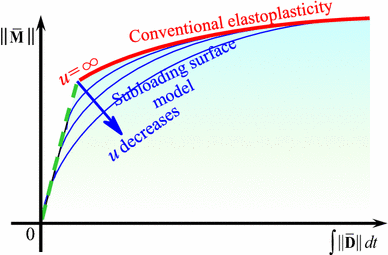
Influence of material parameter u on stress-strain curve
-
2.
The continuity and the smoothness conditions [21, 22, 24] are satisfied, while these conditions are violated in all of the other models assuming the yield surface enclosing the purely-elastic domain.
-
3.
Plastic strain rate can be described even for low stress level and for cyclic loading process under small stress amplitudes since a purely-elastic domain is not assumed.
-
4.
The yield-judgment whether or not the stress reaches the yield surface is unnecessary since the plastic strain rate develops continuously as the stress approaches the normal-yield surface. In contrast, the yield judgment is required in all of the other elastoplastic models since they assume a surface enclosing a purely-elastic domain.
-
5.
The stress is automatically pulled-back to the normal-yield surface when it goes out from the surface in numerical calculation because of \( \dot{R} < 0 \) for \( R \text{> 1} \) from Eq. (66) with Eq. (67)4 as seen in Fig. 8. In contrast, the particular operation to pull-back the stress to the yield surface is required in all of the other models because they assume a surface enclosing a purely-elastic domain.
Fig. 8 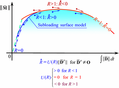
Stress is automatically controlled to be attracted to yield surface in subloading surface model


For the concise illustration of the above-mentioned feature of the subloading surface model, let the stress versus strain relation in the uniaxial loading for the isotropic Mises material with the yield condition \( \sqrt {3/2} \left\| {{\varvec{\upsigma}}{'} } \right\| = F \) be shown in the current configuration. The relations of the axial Cauchy stress σa and the normal-yield ratio R versus the axial strain ɛa ≡ ∫ dadt are depicted in Fig. 9. The responses adopting the linear isotropic hardening \( F= F_{0} + h_{c} \varepsilon^{ep} \) (hc: material constant, ɛep ≡ ∫d p a dt) are depicted in Fig. 9a and those for the nonlinear isotropic hardening rule \( F(H) = F_{0} \{ 1 + h_{1} [1 - \exp ( - h_{2} \varepsilon^{ep} )]\} \) are shown in Fig. 9b. The two levels of axial strain increment \( \, d\varepsilon_{a}\) = 0.0006 and 0.0055 are input in the numerical calculations. Here, any special algorithm for pulling back the stress to the yield surface is not introduced. The material parameters are chosen as follows:

Numerical accuracies of the conventional model and the subloading surface model: uniaxial loading behavior of Mises material with isotropic hardening. a Linear isotropic hardening. b Nonlinear isotropic hardening
Material constants:
Initial values:
The nonsmooth curves bent at the yield point are expressed by the conventional model. Moreover, the stress deviates from the exact curve of the concventional elastoplasticity. The deviation becomes larger with the increases in the nonlinearity of hardening and in the increase of input strain increment. On the other hand, the stress is automatically attracted to the normal-yield surface in the subloading subloading surface model even for the quite large strain increment \( \, d\varepsilon_{a} = 0 \text{.0055}\, \text{(0}{.55\% )} \). The zigzag lines tracing the exact curve are calculated such that the stress rises up when it lies below the normal-yield surface but it drops down immediately if it goes over the normal-yield surface, obeying the evolution rule of normal-yield ratio in Eq. (66) with Eq. (68), i.e. \( \dot{R}>0\,{\text{for}}\, \, R< 1 \) and \( \dot{R} < 0{\text{for }}R> 1 \). The amplitude of zigzag decreases gradulally in the monotonic loading process, while, needless to say, the amplitude is smaller for a smaller input increment of strain. Eventually, the subloading surface model posseses the distinguished high ability for numerical calculation as verified also quantitatively in these concrete examples, which cannot be attained in any other elastoplastic constitutive models including the conventional model and the cyclic kinematic hardening models.
8 Multiplicative Hyperelastic-Based Plastic Equation Incorporating Extended Subloading Surface Model
The initial subloading surface model is furnished with the distinguished ability improving the conventional elastoplastic model as described in the last section. However, it is incapable of describing the cyclic loading behavior, predicting open hysteresis loops because only elastic deformation is induced in the unloading process. Then, it has been extended such that the similarity-center of the normal-yield and the subloading surfaces moves with the plastic deformation, while the similarity-center is regarded as the elastic-core because the most elastic deformation behavior is induced when the stress lies on it, the normal-yield ratio reducing to zero, i.e. the subloading surface reducing to a point.
8.1 Basic Feature of Extended Subloading Surface Model in Current Configuration
The uniaxial loading behavior is depicted in Fig. 10 in the current configuration for the Mises material without a hardening (F = F0 and \( {\varvec{\upalpha}} = {\mathbf{O}} \)) for simplicity. Here, \( {\bar{\varvec{\upalpha }}} \) is the conjugate point in the subloading surface to the kinematic hardening variable (back stress) \( {\varvec{\upalpha}} \) in the normal-yield surface. The elastic-core \( {\mathbf{c}} \) goes up following the stress by the plastic strain rate in the initial loading process as seen in Fig. 10a, b. The subloading surface shrinks and thus only elastic strain rate is induced until the stress goes down to the elastic-core in the unloading process as seen in Fig. 10c. After that the subloading surface begins to expand and thus the plastic strain rate in the compression is induced in the unloading-inverse loading process whilst the similarity-center goes down following the stress by the plastic strain rate as seen in Fig. 10d. Again only the elastic strain rate is induced until the stress goes up to the similarity-center in the reloading process from the complete unloading as seen in Fig. 10e. After that the subloading surface begins to expand and thus the plastic strain rate is induced whilst the similarity-center goes up following the stress by the plastic strain rate as seen in Fig. 10f. The expanded figure of Fig. 10f is shown in the lowest part of Fig. 10. Consequently, the closed hysteresis loop is depicted realistically as shown in this figure.

Prediction of uniaxial loading behavior by extended subloading surface model in current configuration: a initial state, b initial loading process, c unloading process until similarity-center, d unloading-inverse loading process after passing similarity-center, e reloading process until reaching elastic-core and f reloading process (——— Stress, — — — Elastic-core, - - - - - - - - Center of subloading surface)
The extended subloading surface model would describe the cyclic loading behavior realistically as illustratively shown in Fig. 11. It does not contain any drawbacks in the cyclic plasticity models based on the kinematic hardening concept, while the continuity and the smoothness conditions [21, 22, 24] are satisfied only in this model. Then, it has been applied to the descriptions of rate-independent and rate-dependent elastoplastic deformation behavior of not only metals but also soils and further the friction phenomena between solids as will be described in detail in the later sections.

Modification of subloading surface model to describe cyclic loading behavior
The elastoplastic models other than the subloading surface model, i.e. the conventional model and the cyclic kinematic hardening models are incapable of describing monotonic loading behavior realistically and also cyclic loading behavior appropriately as was described in the foregoing. In addition, it would be incapable of formulating multiplicative hyperelastic-based plastic equation based on them. Only the extended subloading surface model with the translation of the elastic-core is capable of describing the monotonic and cyclic loading behavior rigorously and can be led to the multiplicative hyperelastic-based plasticity as will be described in detail in the subsequent sections.
The normal-yield, subloading and elastic-core surfaces in the current configuration is shown in Fig. 12. The variables in the hypoelastic-based plasticity correspond to the variables in the intermediate configuration for the multiplicative hyperelastic-based plasticity as follows:
\( {\bar{\mathbf{M}}}_{c} \) is the elastic-core, i.e. the similarity-center of the subloading surface to the normal-yield surface. \( \bar{\underset{\raise0.3em\hbox{$\smash{\scriptscriptstyle-}$}}{\mathbf{M}}}_{k} \) is the conjugate point in the subloading surface to the kinematic hardening variable \( {\bar{\mathbf{M}}}_{k} \) in the normal-yield surface. The variables \( {\bar{\mathbf{M}}}_{k} \) and \( {\bar{\mathbf{M}}}_{c} \) leading to the anisotropy are the symmetric tensors, although the Mandel stress \( {\bar{\mathbf{M}}} \) is the asymmetric tensor in general.

Normal-yield, subloading and elastic-core surfaces in current configuration. a General case. b Mises material
The evolution rule of the elastic-core, i.e. the similarity-center \( {\mathbf{c}} \) of the normal-yield and the subloading surfaces in the infinitesimal elastoplasticity is given as follows [66]:
where c is the material parameters and \( {\bar{\mathbf{n}}} \) is the normalized outward-normal of the subloading surface, i.e.
\( {\bar{\varvec{\upalpha }}} \) is the conjugate point in the subloading surface to \( {\varvec{\upalpha}} \) in the normal-yield surface. The elastic-core surface which passes through the elastic-core and is similar to the normal-yield surface with respect to the back-stress \( {\varvec{\upalpha}} \) is given as follows (Fig. 12):
where
\( \Re_{c} { (0} \le \Re_{c} \le 1 ) \) is called the elastic-core yield ratio designating the ratio of the size of the elastic-core surface to that of the normal-yield surface, i.e. the approaching-degree of the elastic-core to the normal surface, and \( \chi { ( < 1)} \) is the material parameter designating the limit value of ℜc. \( {\hat{\mathbf{n}}}_{c} \) is the normalized outward-normal of the elastic-core surface, i.e.
The following inequality holds for Eq. (78).
Therefore, the elastic-core does not go out from the limit elastic-core surface\( f({\hat{\mathbf{c}}})= \chi F(H) \) (see Fig. 12).
The validity of the extended subloading surface model in the hypoelastic-based plasticity has been verified widely (cf. e.g. [33, 43, 45]).
8.2 Multiplicative Decomposition of Plastic Deformation Gradient for Elastic-Core
Analogously to the multiplicative decomposition of the plastic deformation gradient for the kinematic hardening in Eq. (3), decompose \( {\mathbf{F}}^{p} \) into the plastic storage part \( {\mathbf{F}}_{cs}^{p} \) causing the translation of the elastic-core and its plastic dissipative part \( {\mathbf{F}}_{cd}^{p} \) multiplicatively as follows [29, 30]:
The configurations based on these decompositions are illustrated in Fig. 13.

Multiplicative decompositions of deformation gradient tensor for material with translations of kinematic hardening variable and elastic-core
The following tensors of the storage part \( {\mathop{{\mathbf{C}}}\limits^{\smile}{}_{cs}^{p}}\equiv {\mathbf{F}}_{cs}^{pT} {\mathbf{F}}_{cs}^{p} \) and the dissipative part \( {\mathop{{\mathbf{C}}}\limits^{\smile}{}_{cd}^{p}}\equiv {\mathbf{F}}_{cs}^{pT} {\mathbf{F}}_{cd}^{p} \) are defined.
where one has
Tensor variables in the elastic-core intermediate configuration are specified by adding the hat symbol \( {({}^{\mathop{\overset{\lower0.2em\hbox{$\smash{\scriptscriptstyle\smile}$}}{}}\limits^{{}}})} \).
Further, the following additive decomposition of the velocity gradient holds for the elastic-core analogously to Eqs. (15)–(19) for the kinematic hardening variable.
where
noting
The material-time derivative of \( {\mathop{{\mathbf{C}}}\limits^{\smile}{}_{ks}^{p}} \) in Eq. (5) is given by
8.3 Elastic-Core
The contravariant push-forward of the 2nd Piola–Kirchhoff stress-like variable for the elastic-core \( {\mathbf{\overset{\lower0.2em\hbox{$\smash{\scriptscriptstyle\smile}$}}{S} }}_{c}^{{}} \) from \( \overset{\lower0.5em\hbox{$\smash{\scriptscriptstyle\smile}$}}{\mathcal{K}} \) to \( \bar{\mathcal{K}} \) is given by
Further, the Mandel-like variable \( {\bar{\mathbf{M}}}_{c} \) for the elastic-core is given by
noting Eq. (87). Note here that the Mandel stress \( {\bar{\mathbf{M}}} \) is the asymmetric tensor in general but the Mandel-like elastic-core \( {\bar{\mathbf{M}}}_{c} \) is the symmetric tensor.
The material-time derivative of \( {\bar{\mathbf{M}}}_{c} \) is given analogously to Eq. (26) for that of the kinematic hardening as follows:
8.4 Hyperelasticity for Elastic-Core
Further, let \( {\mathop{{\mathbf{S}}}\limits^{\smile}{}_{c}}\) be formulated incorporating the strain energy function \( \psi^{c} ({\mathop{{\mathbf{C}}}\limits^{\smile}{}_{cs}^{p}} )\) as
from which \( {\bar{\bar{\mathbf{S}}}}_{c} \) and \( {\bar{\mathbf{M}}}_{c} \) are given by
noting Eqs. (87), (93) and (96).
The material-time derivative of \( {\mathbf{\overset{\lower0.5em\hbox{$\smash{\scriptscriptstyle\smile}$}}{S} }}_{c} \) is given from Eq. (96) with Eq. (92) as
where
Substituting Eq. (98) into Eq. (95), \( {\dot{\bar{\mathbf{M}}}}_{c} \) is given as follows:
8.5 Normal-Yield, Subloading and Elastic-Core Surfaces
The subloading surface in Eq. (65) for the initial subloading surface model is extended as follows:
in the intermediate configuration, which are depicted in Fig. 14.

Normal-yield, subloading and elastic-core surfaces in the intermediate configuration. a General case. b Mises material
The subloading surface is given from Eq. (101) with Eq. (77) as follows:
from which the normal-yield ratio R is calculated.
The material-time derivative of the kinematic hardening variable \( \bar{\underset{\raise0.3em\hbox{$\smash{\scriptscriptstyle-}$}}{\mathbf{M}}}_{k} \) is given by
leading to
The elastic-core surface which passes through the elastic-core \( {\bar{\mathbf{M}}}_{c} \) and is similar to the normal-yield surface with respect to the back-stress \( {\bar{\mathbf{M}}}_{k} \) in the hyperelastic-based plasticity is given noting Eq. (81) as follows:
8.6 Plastic Flow Rules
The plastic strain rate is given in the following associated flow rule proposed by Hashiguchi [29, 30].
where \( \dot{\bar{\lambda }} \) is the positive plastic multiplier and
which is the normalized and symmetrized tensor. If the strain energy functions ψe is given by invariants of \( {\bar{\mathbf{C}}}^{e} \) leading to the elastic isotropy, the symmetries of the Mandel stress \( {\bar{\mathbf{M}}}= {\bar{\mathbf{M}}}^{T} \) holds resulting in the symmetry \( \partial f(\bar{\underset{\raise0.3em\hbox{$\smash{\scriptscriptstyle-}$}}{\mathbf{M}}})/\partial {\bar{\mathbf{M}}}= (\partial f(\bar{\underset{\raise0.3em\hbox{$\smash{\scriptscriptstyle-}$}}{\mathbf{M}}})/\partial {\bar{\mathbf{M}}})^{T} \).
The dissipative parts of the plastic velocity gradient for the kinematic hardening variable and the elastic-core are given from Eqs. (42) and (78) as follows:
where
In order to describe a higher tangent modulus in the reloading process than in the unloading process, e.g. the generalized Masing effect [62], the material parameter u is extended to
where \( \bar{u} \) and uc are material constants, ℜc is given by Eq. (105) and Cσ is given as follows [27, 31]:
Cσ is larger when the direction of the plastic strain rate is nearer to the outward-normal of the elastic-core surface, and thus u is larger in the reloading process and smaller in the reverse loading process.
Let the plastic spin \( {\bar{\mathbf{W}}}^{p} , \) the kinematic-hardening spin \( \mathop{{\mathbf{W}}}\limits^{\frown}{}_{kd}^{p} \) and the elastic-core spin \(\mathop{{\mathbf{W}}}\limits^{\smile}{}_{cd}^{p} \) be given extending the equation in the hypoelastic-based plasticity by Zbib and Aifantis [92] and incorporating Eqs. (106), (108) and (109) as follows:
where η p c is the material parameter. The plastic spin tensor \( {\bar{\mathbf{W}}}^{p} \) diminishes if the symmetry of the Mandel stress, i.e. \( {\bar{\mathbf{M}}} = \bar{{\bf M}}^{T} \) due to the elastic isotropy and the plastic isotropy due to \( {\bar{\mathbf{M}}}_{k} = {\bar{\mathbf{M}}}_{c} = {\mathbf{O}} \) hold. Further, the spin tensors \( {\bar{\mathbf{W}}}_{kd}^{p} \) and \( {\bar{\mathbf{W}}}_{cd}^{p} \) diminish for the plastic-isotropy due to \( {\bar{\mathbf{M}}}_{k} = {\bar{\mathbf{M}}}_{c} = {\mathbf{O}} \).
The velocity gradients are given by substituting Eqs. (106), (108), (109) and (113) into Eqs. (11)3, (16)2 and (89)2 as follows:
The substitutions of Eq. (114) into Eqs. (29), (36) and (100) yield:
8.7 Plastic Strain Rate
The elastic constitutive equation is given by Eqs. (27)–(29). The plastic strain rate will be formulated in this section. The formulations given in this section is not necessary in the numerical calculation by the return-mapping based on the closet-point projection.
The time-differentiation of Eq. (101) leads to the consistency condition of the subloading surface as follows:
It holds from Eq. (101) that
by the Euler’s theorem for the homogenous function \( f(\bar{\underset{\raise0.3em\hbox{$\smash{\scriptscriptstyle-}$}}{\mathbf{M}}}) \) of \( \bar{\underset{\raise0.3em\hbox{$\smash{\scriptscriptstyle-}$}}{\mathbf{M}}} \) in degree-one, and then it follows that
which leads to
where
The substitution of Eq. (120) into Eq. (118) leads to
The further substitution of Eq. (104) into Eq. (122) leads to
Furthermore, substituting the relation
Equation (123) is rewritten as
where
based on Eqs. (57) and (66) with Eq. (106).
The substitutions of Eqs. (116), (117), (126) and (127) into Eq. (125) lead to the consistency condition:
from which it follows that
where
The substitution of Eq. (115) into Eq. (128) leads to the consistency condition:
using the symbol \( \dot{\bar{\varLambda }} \) for the plastic multiplier in terms of the strain rate instead of \( \dot{\bar{\lambda }} \) in terms of the stress rate. The plastic multiplier is given from Eq. (131) as follows:
The loading criterion is given by
which can be given actually as
9 Material Functions
Material functions contained in the constitutive equations formulated in the preceding sections are given for metals and soils in this section.
9.1 Metals
The hyperelastic equation and the yield functions for metals are shown below in the intermediate configuration.
9.1.1 Hyperelastic Equations
The hyperelastic equations are given for the stress, the kinematic hardening variable and the elastic-core.
9.1.1.1 Stress
The following strain energy function of elastic deformation in the Modified Neo-Hookean elasticity may be adopted [84, 85].
where μ and Λ are the material constants. The substitution of Eq. (135) into Eq. (27) reads:
noting
It is followed from Eq. (136) that
where \( {\mathbf{g}}={\mathbf{F}}^{e-T} {\bar{\mathbf{G}}}{\mathbf{F}}^{eT} \) is the metric tensor in the current configurations.
The hyperelastic tangent modulus tensor \( {\bar{\mathbb{C}}}^{e} \) in Eq. (31) is given for Eq. (136) by
where \( {\bar{\boldsymbol{\mathfrak{C}}}}^{e} \) is the fourth-order tensor defined as
which possesses the minor symmetry \( \bar{\mathfrak{C}}_{ijkl}^{e} = \bar{\mathfrak{C}}_{jikl}^{e} = \bar{\mathfrak{C}}_{ijlk}^{e} \) and the major symmetry \( \bar{\mathfrak{C}}_{ijkl}^{e} = \bar{\mathfrak{C}}_{klij}^{e} \).
9.1.1.2 Kinematic Hardening Variable
Assume the following strain energy function for kinematic hardening, which possesses the identical form to the shear part in Eq. (135).
where Ck is material constant. It is derived from Eq. (32) that
Then, the Mandel-like kinematic hardening variable is given from Eqs. (33) and (143) as follows:
noting
\( \mathop{\mathbb{C}}\limits^{\frown}{}^{k} \) in Eq. (35) is given for Eq. (143) as
9.1.1.3 Elastic-Core
Assume the following strain energy function for elastic-core analogously to the kinematic hardening variable described in 9.1.2.
where Cc is material constant. The following relations hold.
\( \mathop{{\mathbb{C}}}\limits^{\smile}{}^{c} \) in Eq. (99) is given for Eq. (146) as
9.1.2 Yield Functions
Assume the von Mises yield function and the plastic equivalent hardening, i.e.
for which we have
F → (1 + h1)F0 holds for H → ∞ in Eq. (151). It follows for Eq. (150) that
The subloading surface for the normal-yield surface in Eq. (150) is given noting Eq. (101), i.e. (102) by the following equation.
i.e.
from which the normal-yield yield ratio is given by
9.2 Soils
The hyperelastic equation and the yield functions for soils are shown below in the intermediate configuration.
9.2.1 Hyperelastic Equation
The hyperelastic constitutive equation of soils was proposed first by Houlsby [48] and it has been extended to various multiplicative hyperelastic equations by Borja and Tamagnini [5], Callari et al. [9], etc. using the Hencky (logarithmic) strain in the current configuration and by Yamakawa et al. [90] using the second Piola–Kirchhoff stress in the intermediate configuration, while they involve various impertinences or incompleteness. The hyperelastic equation within the framework of the multiplicative finite strain theory for soils was shown by Hashiguchi [33] but it involves some impertinences. The exact equation will be shown in the following [37]:
The isotropic hyperelastic equation is given by introducing the function of the variables lnJe and \( \text{tr}{\bar{\underset{\raise0.3em\hbox{$\smash{\scriptscriptstyle-}$}}{\mathbf{C} }}}^{e} \) (\( \text{tr}{\bar{\underset{\raise0.3em\hbox{$\smash{\scriptscriptstyle-}$}}{\mathbf{C} }}}^{e} - 3 \) in detailed expression) which stand for the volumetric strain and deviatoric strain, respectively, as follows:
where
\( {\mathbf{F}}_{vol}^{e} \) is the volumetric part and \( {\mathbf{\underset{\raise0.3em\hbox{$\smash{\scriptscriptstyle-}$}}{F} }}^{e} \) is the so-called unimodular tensor designating the isochoric (constant volume, i.e. deviatoric) part of \( {\mathbf{F}}^{e} \). In addition, \( \text{tr}{\bar{\underset{\raise0.3em\hbox{$\smash{\scriptscriptstyle-}$}}{\mathbf{C} }}}^{e} = \text{3 (}{\mathbf{F}}^{e} = {\mathbf{F}}_{vol}^{{{e} }} ) \) and \( \ln J^{e} = 0\,{ (}{\mathbf{F}}^{e} = {\mathbf{\underset{\raise0.3em\hbox{$\smash{\scriptscriptstyle-}$}}{F} }}^{e} ) \) is required in the purely volumetric deformation and the purely deviatoric deformation, respectively.
The following partial derivatives hold.
noting
The substitution of Eq. (159) into Eq. (157) reads:
Let the following strain energy function be assumed.
noting
where \( \bar{P}_{M0} \) is the initial value of the pressure defined in terms of the Mandel stress \( {\bar{\mathbf{M}}} \), i.e. \( \bar{P}_{M} \equiv -\text{(1/3)tr}{\bar{\mathbf{M}}} \). \( \tilde{\lambda } \) and \( \tilde{\kappa } \) are the material constants standing for the inclinations of the isotropic and the swelling lines in the both logarithmic linear relation of pressure and the volume (cf. [33]). \( \vartheta \text{(<1/2)} \) is material constant, while the volume becomes infinite as the pressure approaches ϑF, while the hardening function F coincides to the preconsolidation pressure in the isotropic consolidation process. G0 is the initial value of elastic shear modulus, n standing for the pressure-dependence of the shear modulus.
The following partial derivatives hold for Eq. (161).
noting \( \partial J^{{e^{{ - n/\tilde{\kappa }}} }} /\partial \ln J^{e} = - (n/\tilde{\kappa })J^{{e - n/\tilde{\kappa }}} \).
Equation (160) with Eq. (162) reads:
from which the Mandel stress is given as follows:
noting \( J^{{e - 2/3}} {\bar{\mathbf{C}}}^{e\prime} = \bar{\underset{\raise0.3em\hbox{$\smash{\scriptscriptstyle-}$}}{\mathbf{C} }}^{e\prime} \) by virtue of Eq. (158)7.
It is follows from Eq. (164) that
i.e.
and
which would describe appropriately the basic characteristics in the volumetric and the deviatoric deformations.
Equations (164), (166) and (167) are rewritten as
with
and
in the current configuration, where \( {\varvec{\uptau}} \) is the Kirchhoff stress tensor, pτ0 is the initial value of \( p_{\tau } \equiv -(\text{tr}{\varvec{\uptau}})/3 \) and \( {\mathbf{\underset{\raise0.3em\hbox{$\smash{\scriptscriptstyle-}$}}{b} }}^{e} \) is the elastic unimodular left Cauchy–Green deformation tensor, i.e.
The above-mentioned elastic equation is reduced to the infinitesimal strain theory by adopting the strain energy function
as follows:
resulting in
i.e.
and
where p is the pressure, i.e. \( p \equiv - ( \text{tr}{\varvec{\upsigma}} \text{)/3} \) and its initial value is denoted by p0. \( {\varvec{\upvarepsilon}}^{e} \) is the infinitesimal elastic strain tensor and \( \varepsilon_{v}^{e} \cong \text{tr}{\varvec{\upvarepsilon}}^{e} , \)\( \varepsilon_{d}^{e} = \left\| {{\varvec{\upvarepsilon}}^{e\prime}} \right\| \).
The elastic balk modulus K and the elastic shear modulus G adopted in the hypoelasticity for the above-mentioned elastic equations are given as follows:
where \( d_{v}^{e} \equiv \text{tr}\varvec{l}^{e} , \, {\mathbf{d}}^{e} \equiv \text{sym}[\varvec{l}^{e} ] \), while \( n \cong 0 \text{.5} \) can be chosen in most of soils [82].
The elastic constitutive equations of soils formulated above possess the following physical validities.
-
1.
It is applicable up to the finite deformation/rotation.
-
2.
It is applicable up to the negative pressure range which depends on the preconsolidation pressure.
-
3.
The shear modulus increases depending on the pressure.
-
4.
They are consistent for the multiplicative hyperelasticity, the infinitesimal hyperelasticity and the hypoelasticity.
9.2.2 Yield Functions
The modified Cam-clay yield surface [8, 72], which is exhibited as the ellipsoid passing through the origin and possessing the long axis coinciding to the hydrostatic axis in the three-dimensional stress space, was extended by Hashiguchi and Mase [39] as follows (Fig. 15):
where F is the isotropic hardening function corresponding to the long axis of the ellipsoidal yield surface, \( \xi_{h}\, { ( < }\vartheta ) \) is the material constant describing the translation to the negative pressure range by ξhF along the hydrostatic direction and M is the ratio of the short axis to the long axis, which is the function of the Lode angle as follows [25]):
where ϕc is the friction angle in the tri-axial compression sate, while \( M_{c} \equiv 2\sqrt 6 \sin \phi_{c} /(3 - \sin \phi_{c} ) \) is the value of M in that state (θM = π/3), and

Yield surface of soils with tensile strength
Equation (178) is expressed in the separated form of the function \( f(\bar{P}_{M} ,X ) \) of the stress and the hardening function F, i.e.
where
The isotropic hardening function is given as [23].
where \( J^{p} = \mathbf {\det{F}}^{p} \) and F0 is the initial value of F.
10 Calculation Procedures
The calculation procedure by the above-mentioned formulations is described in this section.
First, the plastic multiplier \( \dot{\bar{\varLambda }} \) is calculated by the input of the velocity gradient \( {\bar{\mathbf{L}}} \) into Eq. (62), while \( {\bar{\mathbf{L}}} \) is calculated from the current velocity gradient \( \varvec{l} \) by Eq. (10). Then, substituting it into Eq. (114), the plastic and the dissipative parts \( {\bar{\mathbf{L}}}^{p} \), \( {\bar{\mathbf{L}}}_{kd}^{p} \) and \( {\bar{\mathbf{L}}}_{cd}^{p} \) are calculated. On the other hand, the plastic multiplier \( \dot{\bar{\varLambda }} \) is calculated directly from the plastic flow rule in Eq. (106) and the stress rate is calculated by Eq. (29) under \( {\bar{\mathbf{L}}} = \mathbf {O}\) in the plastic corrector process in the return-mapping method. Thereafter, the stress and the tensor-valued internal variables are calculated by the process described below.
The deformation gradient tensor is updated by
where
with the displacement vector \( {\mathbf{u}} \), designating \( {\boldsymbol{\nabla }}_{{{\mathbf{x}}_{n} }} \equiv \partial ( \, )/\partial {\mathbf{x}}_{n} \) and noting
The rates of the plastic gradient and its dissipative parts are given from Eqs. (10)3, (18) and (91) as follows:
where \( {\bar{\mathbf{L}}}^{p} \), \( {\bar{\mathbf{L}}}_{kd}^{p} \) and \( {\bar{\mathbf{L}}}_{cd}^{p} \) are given by Eq. (114). The storage parts \( {\mathbf{F}}^{e} , \, {\mathbf{F}}_{ks}^{p} \) and \( {\mathbf{F}}_{cs}^{p} \) of the deformation gradient are given by substituting the results of the time-integrations of Eq. (188) into
Further, \( {\bar{\mathbf{C}}}^{e} ,\mathop{{\mathbf{C}}}\limits^{\frown}{}_{ks}^{p} \) and \( \mathop{{\mathbf{C}}}\limits^{\smile}{}_{cs}^{p} \) are calculated by substituting Eq. (189) into Eqs. (5) and (86). Further, the stress \( {\bar{\mathbf{S}}} \), the kinematic hardening variable \( {\mathbf{\overset{\lower0.2em\hbox{$\smash{\scriptscriptstyle\frown}$}}{S} }}_{k}^{{}} \) and the elastic-core \( {\mathbf{\overset{\lower0.2em\hbox{$\smash{\scriptscriptstyle\smile}$}}{S} }}_{c}^{{}} \) are calculated by substituting \( {\bar{\mathbf{C}}}^{e} ,\mathop{{\mathbf{C}}}\limits^{\frown}{}_{ks}^{p} \) and \(\mathop{{\mathbf{C}}}\limits^{\smile}{}_{cs}^{p}\) into Eqs. (27), (32) and (96). The isotropic hardening variable and the normal-yield ratio are calculated by the time-integration of Eqs. (126) and (127).
The plastic constitutive equation with the plastic modulus in Eq. (130) is not necessary to be used in the numerical calculation by the return-mapping in which the plastic strain rate is calculated by use of only the plastic flow rule in Eq. (106) and then the stress and internal variables are calculated by the procedures described above.
The time-integrations of Eq. (188) for the tensors \( {\mathbf{F}}^{p} \), \( {\mathbf{F}}_{kd}^{p} \) and \( {\mathbf{F}}_{cd}^{p} \) can be executed in high efficiency by the tensor exponential method [46, 65, 88] which is delineated below.
The equations in Eq. (188) are collectively described in terms of an arbitrary second-order tensors \( {\mathbf{T}} \) and \( {\mathbf{Z}} \) as follows:
Consider the following candidate as the numerical solution of Eq. (190) for the time-interval \( \Delta t = [t_{n} , \, t_{n + 1} ] \).
provided that \( {\mathbf{Z}} \) and \( {\mathbf{T}}_{n} \) are constant during the time-interval. The time-differentiation of Eq. (191) leads to
coinciding to Eq. (190) and thus the rightness of the candidate in Eq. (191) is proven. The tensor \( {\mathbf{Z}} \) is given by \( {\bar{\mathbf{L}}}^{p} \), \( \mathop{{\mathbf{L}}}\limits^{\frown}{}_{kd}^{p} \) and \( \mathop{{\mathbf{L}}}\limits^{\smile}{}_{cd}^{p} \) for \( {\mathbf{F}}^{p} \), \( {\mathbf{F}}_{kd}^{p} \) and \( {\mathbf{F}}_{cd}^{p} \), respectively, as shown in Eq. (188).
11 Loading Criterion in Return-Mapping for Subloading Surface Model
The subloading surface model is capable of describing not only the monotonic but also the cyclic and the non-proportional loading behaviors, since the yield surface enclosing the purely-elastic domain is not incorporated in this model. However, the particular attention is required for the return-mapping method in numerical calculations for this model, in which rather large loading increments are input in the elastic trial step. In fact, there exists the possibility of the occurrence of plastic strain increment even when the stress increment is directed inward of the subloading surface. Therefore, a particular loading criterion after the elastic trial step and a particular calculation procedure in the initiation of plastic corrector step are required in the return-mapping projection for the subloading surface model. This fact has not been recognized in the past formulations [2, 16, 28, 33, 46, 90] and the inexact loading criterions after the elastic trial step have been shown in the past [32, 49]. The closet point projection in the return-mapping method for the extended subloading surface model was proposed first by Anjiki et al. [2] and subsequently Iguchi et al. [49] in the multiplicative decomposition and followed the results of Anjiki et al. [2] later by Fincato and Tsutsumi [16].
The exact loading criterion after the elastic trial step and the initial treatment in the plastic corrector step for the subloading surface model will be formulated below extending the former equations in the current configuration [36] to the equations in the intermediate configuration within the framework of the multiplicative elastoplaticity.
11.1 Formulation of Loading Criterion
Consider the loading criterion at the initial stage of the plastic corrector step. The following facts should be noticed, referring to Fig. 16, where the elastic trial steps for the initial subloading surface model \( ({\bar{\mathbf{M}}}_{c} = {\bar{\mathbf{M}}}_{k} ) \) and the extended subloading surface model \( ({\bar{\mathbf{M}}}_{c} \ne {\bar{\mathbf{M}}}_{k} ) \) are shown in Fig. 16a, b, respectively, designating the kinematic hardening variable and the elastic-core, i.e. the similarity-center of the normal-yield and the subloading surfaces by \( {\bar{\mathbf{M}}}_{k} \) and \( {\bar{\mathbf{M}}}_{c} \), respectively.

Loading criterion when elastic trial stress is directed inward of subloading surface at step n in return-mapping method
-
1.
The plastic strain increment is obviously induced in the plastic corrector step if the stress increment \( \Delta {\bar{\mathbf{M}}}_{n + 1}^{\text{trial}} \equiv {\bar{\mathbf{M}}}_{n + 1}^{\text{trial}} - {\bar{\mathbf{M}}}_{n} \) in the elastic trial step is directed outward of the subloading surface at the step n, while it is not induced if the stress \( {\bar{\mathbf{M}}}_{n + 1}^{\text{trial}} \) stays inside the elastic response region, i.e. \( f(\bar{\underset{\raise0.3em\hbox{$\smash{\scriptscriptstyle-}$}}{\mathbf{M}}}_{n + 1}^{\text{trial}} ) - R_{e} F(H_{n} ) < 0 \). Here, the stress at the end of the step n and the elastic trail step are denoted by \( {\bar{\mathbf{M}}}_{n} \) and \( {\bar{\mathbf{M}}}_{n + 1}^{\text{trial}} \), respectively, and \( \bar{\underset{\raise0.3em\hbox{$\smash{\scriptscriptstyle-}$}}{\mathbf{M}}}_{n + 1}^{\text{trial}} \) is given by \( \bar{\underset{\raise0.3em\hbox{$\smash{\scriptscriptstyle-}$}}{\mathbf{M}}}_{n + 1}^{\text{trial}} = {\bar{\mathbf{M}}}_{n + 1}^{\text{trial}} - \bar{\underset{\raise0.3em\hbox{$\smash{\scriptscriptstyle-}$}}{\mathbf{M}}}_{n + 1}^{\text{trial}} \) where \( \bar{\underset{\raise0.3em\hbox{$\smash{\scriptscriptstyle-}$}}{\mathbf{M}}}_{n + 1}^{\text{trial}} \) on the subloading surface is the conjugate point of \( {\bar{\mathbf{M}}}_{kn} \) on the normal-yield surface.
-
2.
The plastic strain increment is induced if the stress increment \( \Delta {\bar{\mathbf{M}}}_{n + 1}^{\text{trial}} \) makes the acute angle with the outward-normal of the subloading surface at the elastic trial step even if the stress increment \( \Delta {\bar{\mathbf{M}}}_{n + 1}^{\text{trial}} \) is directed inward of the subloading surface at the final state of the step n, while it is not induced if the stress \( {\bar{\mathbf{M}}}_{{n+ 1}}^{{\text{trial}}} \) stays inside the elastic response region, i.e. \( f(\bar{\underset{\raise0.3em\hbox{$\smash{\scriptscriptstyle-}$}}{\mathbf{M}}}_{n + 1}^{\text{trial}} ) - R_{e} F(H_{n} ) < 0 \).
Then, the loading criterion in the return-mapping method for the subloading surface model is given as follows:

where
11.2 Initiation of Plastic Corrector Step for Mises Material
The following equation holds at the end of the step n for the Mises material.
which is rewritten as
from which Rn is given by
Analogously, the following equation holds at the end of the elastic trial step for the Mises material.
which is rewritten as
from which \( R_{{n+ 1}}^{{\text{trial}}} \) is given by
The plastic corrector step is executed until the subloading surface equation
is satisfied within the prescribed tolerance.
The plastic corrector step is started for the difference from the subloading surface \( f(\bar{\underset{\raise0.3em\hbox{$\smash{\scriptscriptstyle-}$}}{\mathbf{M}}}_{n} ) = R_{n} F(H_{n} ) \) in the end of the step n to the subloading surface \( f(\bar{\underset{\raise0.3em\hbox{$\smash{\scriptscriptstyle-}$}}{\mathbf{M}}}_{{n+ 1}}^{{\text{trial}}} ) = R_{{n+ 1}}^{{\text{trial}}} F(H_{n} ) \) in the elastic trial step for the case 1) ii). On the other hand, it must be executed for the case 2) ii) b) by the special procedures described in the following.
The subloading surface once shrinks inducing only elastic strain increment and turns to expand inducing the plastic strain increment after it contacts tangentially to the stress increment \( \Delta {\bar{\mathbf{M}}}_{{n+ 1}}^{\text{trial}} \) in the process of the stress variation from \( {\bar{\mathbf{M}}}_{n} \) as shown in Fig. 16. Then, we need to calculate the normal-yield ratio \( R_{{n+ 1}}^{0} \) in the state that the subloading surface contacts tangentially to the line-element. Here, the following relations must be satisfied at the contact point, where the stress at the contact point, i.e. the plastic-loading initiation stress is denoted by \( {\bar{\mathbf{M}}}_{{n+ 1}}^{0} \) from which the subloading surface changes from the contraction to the expansion.
where
\( s \text{(0} \le s \le \text{1)} \) is the unknown scalar parameter which must be determined so as to satisfy Eq. (207) at the stress \( {\bar{\mathbf{M}}}_{{n+ 1}}^{0} \). The two unknown variables s and \( R_{{n+ 1}}^{0} \) are involved in Eq. (207). In what follows, the explicit calculation procedure of them will be shown for the Mises material.
Equation (207) is explicitly described for the Mises material with \( f(\bar{\underset{\raise0.3em\hbox{$\smash{\scriptscriptstyle-}$}}{\mathbf{M}}}_{{n+ 1}}^{{0\prime}} ) =\sqrt {3/2} \left\| {\bar{\underset{\raise0.3em\hbox{$\smash{\scriptscriptstyle-}$}}{\mathbf{M}}}_{{n+ 1}}^{{0\prime}} } \right\| \) leading to \( \bar{\underset{\raise0.3em\hbox{$\smash{\scriptscriptstyle-}$}}{\mathbf{N}}}_{{n+ 1}}^{0} = \bar{\underset{\raise0.3em\hbox{$\smash{\scriptscriptstyle-}$}}{\mathbf{M}}}_{{n+ 1}}^{{0\prime}} /\left\| {\bar{\underset{\raise0.3em\hbox{$\smash{\scriptscriptstyle-}$}}{\mathbf{M}}}_{{n+ 1}}^{{0\prime}} } \right\| \) as follows:
i.e.
The upper equation in Eq. (213) is expressed as
leading to
from which we have
The substitution of Eq. (214) into Eq. (213)2 leads to
resulting in
which is the quadratic equation of \( R_{{n+ 1}}^{0} \) (recognized through the discussion with Masanori Oka and Takuya Anjiki (Yanmar Co Ltd.), 2017). Equation (215) is rewritten as
The solution of \( R_{{n+ 1}}^{0} \) in Eq. (215) is given by
where
with
One must choose the solution satisfying \( 0 \le R_{{n+ 1}}^{0} \le 1 \) in Eq. (216). Here, we must set \( R_{{n+ 1}}^{0} = R_{e}\) if \( R_{{n+ 1}}^{0} \le R_{e}\) in the calculated result. It is enough to calculate the initial normal-yield ratio \( R_{{n+ 1}}^{0} \), while it is not necessary to calculate the scalar number s and the stress \( {\bar{\mathbf{M}}}_{{n+ 1}}^{0} \) for the return-mapping calculation.
The plastic strain increment is induced during the variation of normal-yield ratio from \( R_{{n+ 1}}^{0} \) to \( R_{{n+ 1}} \) which is related to the plastic strain increment \( \varepsilon_{{}}^{p} - \varepsilon_{0}^{p} \) as follows:
The plastic strain increment in the initiation of the plastic corrector step is calculated based on the overstress \( {\bar{\mathbf{M}}}_{{n+ 1}}^{{\text{trial}}} - {\bar{\mathbf{M}}}_{{n+ 1}}^{0} \), i.e. the difference from the elastic trial stress \( {\bar{\mathbf{M}}}_{{n+ 1}}^{{\text{trial}}} \) on the subloading surface at \( R_{{n+ 1}}^{{\text{trial}}} \) from the stress \( {\bar{\mathbf{M}}}_{{n+ 1}}^{0} \) on that at \( R_{{n+ 1}}^{0} \). However, if \( R_{{n+ 1}}^{0} <\, R_{e} \), we must put \( R_{{n+ 1}}^{0} = R_{e} \) in Eq. (219).
The loading criterion for the return-mapping method in the initial subloading surface model is given by setting \( {\bar{\mathbf{M}}}_{c} = {\bar{\mathbf{M}}}_{k} \) in the above-mentioned formulations, referring to Fig. 16a.
12 Subloading-Overstress Model Based on Multiplicative Decomposition
The deformation gradient \( {\mathbf{F}} \) is multiplicatively decomposed into the elastic deformation gradient \( {\mathbf{F}}^{e} \) and the plastic deformation gradient \( {\mathbf{F}}^{vp} \) instead of the plastic deformation gradient \( {\mathbf{F}}^{p} \) in the multiplicative elastoplasticity described in the preceding sections. Then, we first adopt the following equation instead of Eq. (1).
Further, the viscoplastic deformation gradient \({\mathbf{F}}^{vp} \) is multiplicatively decomposed into the viscoplastic storage part \({\mathbf{F}}_{ks}^{vp} \) causing the kinematic hardening and its dissipative part \({\mathbf{F}}_{kd}^{vp} \) and into the viscoplastic storage part \({\mathbf{F}}_{cs}^{vp} \) causing the elastic-core and its dissipative part \({\mathbf{F}}_{cd}^{vp} \) multiplicatively as follows:
Then, the following right Cauchy-Green deformation tensors for the viscoplastic deformation are introduced.
The velocity gradient \( \varvec{l} \) in the current configuration is additively decomposed into the elastic and the viscoplastic parts:
where
Further, the velocity gradient \( {\bar{\mathbf{L}}} \) in the intermediate configuration is additively decomposed into the elastic and the plastic parts as follows:
where
from which it follows that
where
The viscoplastic velocity gradient \({\bar{\mathbf{L}}}^{vp}\) is additively decomposed for the kinematic hardening and the elastic-core into the storage and the dissipative parts as follows:
where
The viscoplastic strain rate is given extending the overstress model [70, 71] as follows:
where
or
where \( \bar{\underset{\raise0.3em\hbox{$\smash{\scriptscriptstyle-}$}}{\mathbf{N}}} \) is given by Eq. (107), \( \bar{\mu } \), n and Rm (> 1) are the material parameters, while Rm is the maximum value of R, and
based on Eq. (66), leading to the smooth elastic-viscoplastic transition. Here, the normal-yield ratio R in Eq. (65) is renamed as the subloading-yield ratio and denoted by the symbol \( R_{s} { (0} \le R_{s} \le 1 ) \). Let the function \( U(R_{s} ) \) be given by Eq. (68) with the replacement of R to Rs, i.e.
Rs can be calculated analytically through the integration of Eq. (240)1 with Eq. (241) in the viscoplastic deformation process \( ({\bar{\mathbf{D}}}^{vp} \ne {\mathbf{O}}) \) similarly to Eq. (69) as
under the initial condition \( \varepsilon^{vp} = \varepsilon_{0}^{vp}:R_{s} = R_{{s 0}} \), defining \( \varepsilon^{vp} \equiv \int {\left\| {{\bar{\mathbf{D}}}^{vp} } \right\|dt.} \) Equation (237) or (239) is extended to describe the general rate ranging from the quasi-static to the impact loading, while the past overstress model (Rm − R = 1) is inapplicable to deformation behavior at a high strain rate.
The vscoplastic strain rates for the kinematic hardening and the elastic-core are given extending Eqs. (108) and (109) as follows:
The viscoplastic spin \( {\bar{\mathbf{W}}}^{p} \), the kinematic-hardening viscoplastic spin \( {\bar{\mathbf{W}}}_{kd}^{p} \) and the elastic-core viscoplastic spin \( {\bar{\mathbf{W}}}_{cd}^{p} \) are given extending Eq. (113) as follows:
where \( {\eta^{vp}} \), \( {\eta^{vp}_{k}} \) and \( {\eta^{vp}_{c}} \) are the material parameters.
The velocity gradients are given by substituting Eqs. (237) or (239), (243) and (245) into Eqs. (227)3, (231)2 and (234)2 as follows:
The velocity gradient is given by Eq. (225) with Eqs. (226) and (246) as follows:
which is expressed in the incremental form as follows:
The rate of the viscoplastic gradient is given from Eq. (224)3 as follows:
The time-integration for \( {\mathbf{F}}^{vp} \) can be performed effectively by the tensor exponential method as described for the plastic deformation gradient \( {\mathbf{F}}^{p} \) in the end of Sect. 10. The elastic deformation gradient \( {\mathbf{F}}^{e} \) is given by substituting the time-integration \( {\mathbf{F}}^{vp} \) in Eq. (188) into
Then, \( {\bar{\mathbf{C}}}^{e} \) is calculated by Eq. (5) and further the stresses \( {\bar{\mathbf{S}}} \) and \( {\bar{\mathbf{M}}} \) are calculated by Eqs. (27) and (28) as the hyperelastic relation.
Needless to say, the internal variables \( H, \, {\bar{\mathbf{M}}}_{k} , \, {\bar{\mathbf{M}}}_{c} \) involved in \( \bar{\underset{\raise0.3em\hbox{$\smash{\scriptscriptstyle-}$}}{\mathbf{N}}} \) and Rs evolve by the viscoplastic strain rate \( {\bar{\mathbf{D}}}^{vp} \).
13 Hyperelastic-Based Plastic Constitutive Equation for Subloading-Friction Model
The reduction of the friction coefficient from the static to kinetic friction coefficient and the recovery of the friction coefficient under the reduction of sliding velocity are the fundamental characteristics in friction phenomena, which are recognized widely. Difference of the static and kinetic frictions often reaches up to several tens of percent. The formulation of friction phenomenon taken account of these fundamental friction behavior is of importance for accurate analyses of practical problems in engineering. The constitutive equation of friction describing these behavior has been formulated based on the subloading surface concept [19] and thus it is called the subloading-friction model [33, 40, 41, 44]. However, it has been formulated based on the hypoelastic-based plasticity (e.g. [7, 33, 40, 41, 69]), in which the elastic sliding velocity is limited to be infinitesimal and the cumbersome time-integration of corotational contract stress rate is required.
The subloading-friction model will be improved based on the hyperelastic-based plasticity in this section. It is capable of describing exactly the finite sliding behavior under the finite rotation of contact surface without the cumbersome time-integration of corotational contact stress rate by formulating to relate the contact stress directly to the elastic sliding displacement by the hyperelastic equation. Further, it is extended to be applicable to the general case that the contact surface undergoes the rotation and the deformation.
13.1 Sliding Displacement and Contact Traction Vectors
The sliding displacement vector \( {\bar{\mathbf{u}}} \), which is defined as the sliding displacement of the counter (slave) body to the main (master) body, is orthogonally decomposed into the normal sliding displacement vector \( {\bar{\mathbf{u}}}_{n} \) and the tangential sliding displacement vector \( {\bar{\mathbf{u}}}_{t} \) to the contact surface as follows:
where
\( {\mathbf{n}} \) being the unit outward-normal vector of the surface of main body and
Furthermore, \( {\bar{\mathbf{u}}} \) is decomposed into the elastic sliding displacement \( {\bar{\mathbf{u}}}^{e} \) and the plastic sliding displacement \( {\bar{\mathbf{u}}}^{p} \) as follows:
where
setting
The minus sign is added for \( \bar{u}_{n}^{e} \) to be positive when the counter body approaches the main body. On the other hand, the plastic sliding flow rule will be formulated to fulfill \( {\bar{\mathbf{u}}}_{n}^{p} = {\mathbf{0}} \) in Sect. 13.6.
The contact traction vector\( {\mathbf{f}} \) acting on the main body is additively decomposed into the normal traction vector\( {\mathbf{f}}_{n} \) and the tangential traction vector\( {\mathbf{f}}_{t} \) as follows:
where
The minus sign is added for fn to be positive when the compression is applied to the main body by the counter body.
The contact traction vector \( {\mathbf{f}} \), \( {\mathbf{f}}_{n} \) and \( {\mathbf{f}}_{t} \) are calculated from the Cauchy stress \( {\varvec{\upsigma}} \) applied to the contact surface by virtue of the Cauchy’s fundamental theorem (cf. [33]) as follows:
13.2 Elastic Sliding Displacement
Let the contact traction vector \( {\mathbf{f}} \) be given by the hyperelastic relation with the elastic sliding displacement energy function \( \varphi ({\bar{\mathbf{u}}}^{e} ) \) as follows:
The simplest function \( \partial \varphi ({\bar{\mathbf{u}}}^{e} ) \) is given by the quadratic form:
where the second-order symmetric tensor \( {\bar{\mathbf{E}}} \) is the elastic contact tangent modulus tensor fulfilling the symmetry \( {\bar{\mathbf{E}}}= {\bar{\mathbf{E}}}^{T} \). The substitution of Eq. (264) into Eq. (263) leads to
The inverse relation of Eq. (265) is given by
The elastic contact tangent modulus tensor \( {\bar{\mathbf{E}}} \) is given for the isotropy on the contact surface as follows:
where αn and αt are the normal and tangential contact elastic moduli, respectively. Their values are quite large usually as \( 10^{2} - 10^{5}\,{\text{GPa/mm}}^{3} \) for metals because the elastic sliding is caused by elastic deformations of the surface asperities. Equations (265) and (266) with Eq. (267) leads to
Now, introduce the normalized rectangular coordinate system \( ({\hat{\mathbf{e}}}_{1} , \, {\hat{\mathbf{e}}}_{2} , \, {\hat{\mathbf{e}}}_{3} ) = ({\hat{\mathbf{e}}}_{1} , \, {\hat{\mathbf{e}}}_{2} , \, {\mathbf{n}}) \) fixed to the contact surface, which changes with the rotation of the contact surface. The elastic sliding displacement and the contact traction are described as follows:
Hence, Eq. (265) is described in the simple form as follows:
The sliding velocity vector \( {\dot{\bar{\mathbf{u}}}} \) is the objective vector, since it is not an absolute velocity vector but the mutual velocity vector between surface points on the master and the counter bodies. Therefore, it is not necessary to use a corotational velocity vector but we only have to use the time derivative for the sliding velocity vector. Further, note that one does not need to adopt a corotational rate but one has only to use the time derivative for the contact traction vector \( {\mathbf{f}} \) by the fact: The contact traction \( {\mathbf{f}} \) is calculated from the hyperelastic equation with the substitution of the elastic displacement \( {\bar{\mathbf{u}}}^{e} \) which is obtained by subtracting the plastic displacement vector \( {\bar{\mathbf{u}}}^{p} \) from the displacement vector \( {\bar{\mathbf{u}}} \) as will be explained in Sect. 13.7.
13.3 Normal Sliding-Yield and Sliding-Subloading Surfaces
Assume the following sliding-yield surface with the isotropic hardening/softening, which describes the sliding-yield condition.
μ is the isotropic hardening/softening function denoting the variation of the size of the sliding-yield surface. The friction-yield stress function \( f({\mathbf{f}}) \) for the Coulomb friction law is given by
for which μ specifies the coefficient of friction.
Then, in order to introduce the measure of approaching degree to the sliding-yield surface, renamed the normal sliding-yield surface, let the following subloading-sliding surface passing through the current contact stress and maintaining a similarity to the normal sliding-yield surface be introduced, which plays the general measure of approaching degree of the contact stress to the normal sliding-yield surface (see Fig. 17).
where \( r {(0 \le }r \le \text{1)} \) is the ratio of the size of the subloading surface to that of the normal sliding-yield surface and called the normal sliding-yield ratio, playing the role of the measure of the approaching degree of the contact stress to the normal sliding-yield surface.

Coulomb-type normal sliding-yield and subloading-sliding surfaces
13.4 Evolution Rule of Normal Sliding-Yield Ratio
The evolution rule of the normal sliding-yield ratio is given as follows [33]:
where \( U(r) \) is the monotonically-increasing function of r fulfilling the conditions.
The explicit example of \( \bar{U}(r) \) is
where \( \tilde{u} \) is a material constant. Equation (274) with Eq. (276) can be analytically integrated for the monotonic sliding process as follows:
where \( \bar{u}^{p} { (}= \int {\left\| {{\dot{\bar{\mathbf{u}}}}^{p} } \right\|} \,dt ) \), and \( r_{0} \) and \( \bar{u}_{0}^{p} \) are the initial values of r and \( \bar{u}_{{}}^{p} \), respectively. The adoption of the analytical integration in Eq. (277) would be beneficial for the return-mapping in numerical calculations.
13.5 Evolution rule of sliding-hardening/softening function
Taking account of these facts, the evolution rule of the isotropic hardening/softening function μ is postulated as follows [26, 33, 40]:
where μs and \( \mu_{k } (\mu_{s} \ge \mu \ge \mu_{k} ) \) are material constants designating the maximum and minimum values of μ for the static friction and the kinetic friction, respectively. κ is a material constant specifying the rate of decrease of μ in the plastic sliding process, and ξ is a material constant specifying the rate of recovery of μ as time elapses. The first and second terms in Eq. (278) are relevant to the destruction and reconstruction, respectively, of the adhesion between surface asperities.
13.6 Plastic Sliding Velocity
The time derivative of Eq. (273) leads to the consistency condition
The substitution of Eqs. (274) and (278) into Eq. (279) leads to
Assume that the direction of plastic sliding velocity is tangential to the contact plane and outward-normal to the curve generated by the intersection of the subloading-sliding surface and the constant normal traction plane \( {\mathbf{f}}_{n} = {\text{const.}} \), leading to the tangent associated flow rule (see Fig. 18):
where
with
where \( \dot{\bar{\lambda }} \) and \( {\mathbf{n}}_{t} \) are the magnitude and direction, respectively, of the plastic sliding velocity.

Influence of sliding velocity
The substitution of Eq. (281) into Eq. (280) reads:
i.e.
where
are relevant to the plastic and the creep sliding velocity, respectively.
It is obtained from Eqs. (281) and (285) that
Substituting the rate form of Eqs. (266) and (287) into the rate form of Eq. (254), the sliding velocity is given by
The plastic multiplier in terms of the sliding velocity, denoted by the symbol \( \dot{\bar{\varLambda}} \), is given from Eq. (288) as
The inverse relation Eq. (288) is given by substituting the rate form of Eq. (254) with Eq. (289) into the rate form of Eq. (265) as follows:
The loading criterion is given as follows:
or
Some numerical experiments for the linear sliding process for subloading-friction model formulated above are shown in the following. The seven material constants of μs, μk, κ, ξ, \( \tilde{u} \), αn and αt and the initial value μ0 of the friction coefficient are chosen as follows:
The influence of the sliding velocity on the relation of the traction ratio \( f_{t}^{{}} /f_{n}^{{}} \) versus the tangential sliding displacement \( \bar{u}_{t} \) are shown in Fig. 18, where \( \dot{\bar{u}}_{t} \equiv \|{\dot{\bar{\mathbf{u}}}}_{t} \|\). Smooth transitions from the static friction to the kinetic friction and the decreases of the friction coefficient are depicted. Faster decrease of friction coefficient is shown for higher sliding velocity.
The recovery of the static friction coefficient from the kinetic friction with the elapsed time \( \text{t} \) after the stop of sliding is shown in Fig. 19. In the calculation, the constant sliding velocity \( \dot{\bar{u}}_{t} = 0.1\,{\text{mm/s}} \) is given in the first stage reaching the kinetic friction and then the tangential contact traction is unloaded to zero. After the cessation of sliding for several elapsed times, the same sliding velocity in the first stage is given again. The recovery is larger for a longer stationary time.

Influence of stationary time
13.7 Calculation Procedure
The exact calculation of the contact stress can be performed through the hyperelastic relation, while the cumbersome calculation procedure for the time-integration of the corotational contact stress rate in the hypoelastic relation is not required. It will be shown for the sliding processes under the rotation and under the rotation/deformation of the contact surface in the following.
13.7.1 Sliding Process Under Rotation of Contact Surface
The sliding displacement is calculated by the time-integration of the input value of the sliding rate, i.e. \( {\bar{\mathbf{u}}} = \int {{\dot{\bar{\mathbf{u}}}}dt} \). The plastic sliding displacement is calculated by the time-integration of the plastic sliding rate, i.e. \( {\bar{\mathbf{u}}}^{p} = \int {{\dot{\bar{\mathbf{u}}}}^{p} dt} \) based on Eq. (289). The friction coefficient μ is updated by substituting the plastic sliding rate \( {\dot{\bar{\mathbf{u}}}}^{p} \) and the elapsed time into Eq. (278). Further, the contact traction \( {\mathbf{f}} \) is calculated by the hyperelastic relation in Eq. (263) as
the simplest form of which is given for Eq. (265) as follows:
Therefore, the cumbersome operation for the time-integration of the corotational rate of contact traction is not required. Equation (294) is specialized for Eq. (267) with the elastic modulus tensor in Eq. (267) as follows:
noting
Here, note that the rate form in Eq. (290) is not necessary in the calculation procedure described in this section.
13.7.2 Sliding Process Under Rotation and Deformation of Contact Surface
The above-mentioned calculation procedure is applicable under the restriction that the contact plane rotates but does not deform. In the following, the general calculation method for the contact surface undergoing both the rotation and/or the deformation is described below.
Let the primary bases embedded on the contact surface in the reference and the current configurations be denoted as \( {\{ }{\mathbf{G}}_{i} \} \) and \( {\{ }{\mathbf{g}}_{i} (t)\} \), respectively, (see Fig. 20), and let their reciprocal bases be denoted as \( {\{ }{\mathbf{G}}^{i} \} \) and \( {\{ }{\mathbf{g}}^{i} (t)\} \), while they are related through the deformation gradient tensor \( {\mathbf{F}} \) as follows (cf. [33, 46]):

Variations of embedded base vectors for contact surface undergoing rotation/deformation
Let the reference primary base \( \{ {\mathbf{G}}_{i} \} \) form the normalized orthogonal coordinate system in which \( {\mathbf{G}}_{1} \) and \( {\mathbf{G}}_{2} \) are tangential to the contact surface and \( {\mathbf{G}}_{3} \) is outward-normal to the contact surface of the main body, i.e. \( {\mathbf{G}}_{3} = {\mathbf{N}} \), fulfilling \( \left\| {{\mathbf{G}}_{1} } \right\| = \left\| {{\mathbf{G}}_{2} } \right\| = \left\| {{\mathbf{G}}_{3} } \right\| \)\( ( = \left\| {\mathbf{N}} \right\| ) = { 1} \). Therefore, there does not exist the difference between \( {\{ }{\mathbf{G}}_{i} \} \) and \( {\{ }{\mathbf{G}}^{i} \} \). Here, \( {\mathbf{g}}_{3} (t){ (} = {\mathbf{n}}(t) ) \) is neither a unit vector nor normal to the current contact surface in the general material undergoing the deformation.
The sliding rate \( {\dot{\bar{\mathbf{U}}}} \) and the plastic sliding rate \( {\dot{\bar{\mathbf{U}}}}^{p} \) in the reference configuration are related to \( {\dot{\bar{\mathbf{u}}}} \) and \( {\dot{\bar{\mathbf{u}}}}^{p} \) in the current configuration as
where \( {\dot{\bar{\mathbf{u}}}} \) is known from the nodal sliding rate in FEM and \( {\dot{\bar{\mathbf{u}}}}^{p} \) is calculated from Eq. (289). The friction coefficient μ is updated by substituting the plastic sliding rate \( {\dot{\bar{\mathbf{u}}}}^{p} \) into Eq. (278).
\( {\bar{\mathbf{U}}} \) and \( {\bar{\mathbf{U}}}^{p} \) are calculated by the time-integrations of Eq. (297), i.e.
The elastic sliding displacement \( {\bar{\mathbf{U}}}^{e} \) in the reference configuration is calculated by the following equation, from which the elastic sliding displacement \( {\bar{\mathbf{u}}}e \) in the current configurations is known.
The elastic modulus tensor \( {\bar{\mathsf{E}}} \) in the reference configuration and the elastic modulus tensor \( {\bar{\mathbf{E}}} \) in the current configuration are given noting Eq. (296) as follows:
The contact stress \( {\mathsf{F}} \) in the reference configuration is calculated exploiting the calculated result of Eq. (299) with Eq. (297) as follows:
from which the contact stress \( {\mathbf{f}} \) in the current configuration is calculated as
noting
In the above-mentioned calculation procedure, the calculations of the primary and the reciprocal base vectors are not necessary but we only have to import the deformation gradient tensor \( {\mathbf{F}} \) from the FEM analysis for the deformation/rotation of the main body. The calculation procedure in this subsection includes the former one in Sect. 13.1 without the deformation of the contact surface by setting the deformation gradient to be the rigid-body rotation, i.e. \( {\mathbf{F}}= {\mathbf{R}}^{r} \).
13.8 Subloading-overstress friction model
The subloading-friction model described in the preceding sections will be generalized to describe the rate-dependence in the following [33, 44].
The sliding displacement \({\bar{\mathbf{u}}}\) is decomposed into the elastic sliding displacement \({\bar{\mathbf{u}}}^{e}\) and the viscoplastic sliding displacement \({\bar{\mathbf{u}}}^{vp}\) as follows:
The evolution rule of the isotropic hardening/softening function \({\mu}\) in Eq. (278) is extended as follows:
The viscoplastic sliding rate is given as follows:
where
or
where n and \({r_{m}}\) are the material parameters, while \({r_{m}}\) designates the maximum value of r, \({r_{s}}\,(0\le{r_{s}}\le1)\) is the subloading friction-yield ratio calculated using Eq. (274) with Eq. (275) by replacing r to rs and the plastic sliding velocity \({\dot{\bar{\mathbf{u}}}}^{p}\) to the viscoplastic sliding velocity \({\dot{\bar{\mathbf{u}}}}^{vp}\), i.e.
with
Thus, the viscoplastic sliding is induced by the overstress \(f({\mathbf{f}})-{r_{s}}{\mu}\) from the subloading friction surface:
so that a smooth elastic–viscoplastic transition is described.
The sliding rate and its inverse relation are given by Eqs. (265), (304) and (306) as follows:
The generalized subloading friction model proposed above is referred to as the subloading-overstress friction model, which is capable of describe both of the dry and the fluid friction behaviour. The dry friction behaviour is described by choosing the low value for the material parameter \({r_{m}}\) as \({r_{m}}=1+0\) in Eq. (307) or (308) such that the viscoplastic sliding is induced as the contact stress varies along the normal-friction yield surface, i.e. \({r}\cong{r_{s}}.\)
The deformation behaviour described by the subloading-overstress friction model is schematically shown in Fig. 21 in which the normalized overstress divided by the normal contact stress \(f_{n}\) is written simply by the term “overstress”. The dynamic loading friction-yield ratio r coincides with the subloading friction-yield ratio \(r_{s}\), i.e. \(r=r_{s}\) in quasi-static sliding and increases above \(r_{s}\) with increasing sliding velocity. However, r does not rise above \(r_{m}\), i.e. \(r\le r_{m}\), with the equality \(r=r_{m}\) being realised only for impact sliding.

Response of generalized subloading-friction model
The decrease of friction resistance with the increase of sliding velocity is observed in the dry friction and called the negative rate-sensitivity. Inversely, the increase of friction resistance with the increase of sliding velocity is observed in the fluid friction and called the positive rate-sensitivity.
14 Concluding Remarks
The formulation of the exact multiplicative hyperelastic-based plastic constitutive equation has been desired earnestly during a half century after the proposition of the multiplicative decomposition of the deformation gradient tensor in 1960s. Now, it would have been attained by incorporating the rigorous plastic flow rules and the subloading surface model in this article.
The main results in this article are summarized in the following.
-
1.
The exact multiplicative hyperelastic-based plastic constitutive equations are formulated for the conventional elastoplastic model with the yield surface enclosing the purely elastic domain, the initial subloading surface model and the extended subloading surface model which is capable of describing not only the monotonic but also the cyclic loading behavior under the finite deformation and rotation. Among various cyclic plasticity models only the subloading surface model can be formulated based on the framework of the multiplicative elastoplasticity.
-
2.
These equations are extended to the description of the rate-dependent deformation behavior by incorporating the notion of the overstress. They are applicable to the deformation behavior at the general rate ranging from the quasi-static to the impact deformation behavior.
-
3.
The hyperelastic-based plastic constitutive equation for the subloading-friction model is formulated by extending the hypoelastic-based plastic one. It is applicable to the sliding process in which the contact surface undergoes the rotation. It is further extended to be applicable to the sliding process in which the contact surface undergoes not only the rotation but also the deformation.
-
4.
These equations possess the distinguished ability in numerical calculations by the forward-Euler method such that the stress is automatically pulled-back to the yield surface when it goes out from the yield surface, which is the inherent ability of the subloading surface model.
-
5.
The general loading criterion is formulated, which is applicable not only to the monotonic loading process but also to the reverse loading process, and further the initial treatment in the plastic-corrector step is formulated for the return-mapping method adopting the subloading surface model.
These formulations possess the high numerical efficiency in addition to the rigorous description of mechanical behaviors up to the finite deformation/sliding and rotation. They have been long-awaited in the history of elastoplasticity theory. They will highly contribute to the steady developments of the continuum mechanics and the mechanical design technique in industries.
References
Armstrong PJ, Frederick CO (1966) A mathematical representation of the multiaxial Bauschinger effect. CEGB Report RD/B/N 731 (or in: Materials at High Temperature 24:1–26 [2007])
Anjiki T, Oka M, Hashiguchi K (2016) Elastoplastic analysis by complete implicit stress-update algorithm based on the extended subloading surface model. Trans Jpn Soc Mech Eng. https://doi.org/10.1299/transjsme.16-00029
Belytschko T, Liu WK, Moran B (2014) Nonlinear finite elements for continua and structures, 2nd edn. Wiley, Hoboken
Bonet J, Wood RD (1997) Nonlinear continuum mechanics for finite element analysis. Cambridge Univ. Press, Cambridge
Borja RI, Tamagnini C (1998) Cam-clay plasticity, part III: extension of the infinitesimal model to include finite strains. Comput Methods Appl Mech Eng 155:73–95
Brepols T, Vladimirov IN, Reese S (2014) Numerical comparison of isotropic hypo- and hyperelastic-based plasticity models with application to industrial forming processes. Int J Plast 63:18–48
Buczkowski R, Kleiber C (1997) Elasto-plastic interface model for 3D-frictional orthotropic contact problems. Int J Numer Methods Eng 40:599–619
Burland JB (1965) The yielding and dilatation of clay. Corresp Geotech 15:211–214
Callari C, Auricchio F, Sacco E (1998) A finite-strain Cam-clay model in the framework of multiplicative elasto-plasticity. Int J Plast 14:1155–1187
Chaboche JL, Dang-Van K, Cordier G (1979) Modelization of the strain memory effect on the cyclic hardening of 316 stainless steel. In: Transactions of the 5th international conference on SMiRT, Berlin, Division L. Paper No. L. 11/3
Dafalias YF (1985) A missing link in the macroscopic constitutive formulation of large plastic deformations. In: Sawczuk A, Bianchi G (eds) Plasticity today. International symposium on recent trends and results in plasticity. Elsevier, pp 135–151
Dafalias YF, Popov EP (1975) A model of nonlinearly hardening materials for complex loading. Acta Mech 23:173–192
de Souza Neto EA, Perić D, Owen DJR (2008) Computational methods for plasticity. Wiley, Hoboken
Dettmer W, Reese S (2004) On the theoretical and numerical modelling of Armstrong–Frederic kinematic hardening in the finite strain regime. Comput Methods Appl Mech Eng 193:87–116
Drucker DC (1988) Conventional and unconventional plastic response and representation. Appl Mech Rev (ASME) 41:151–167
Fincato R, Tsutsumi S (2017) Closest-point projection method for the extended subloading surface model. Acta Mech. https://doi.org/10.1007/s00707-017-1926-0
Gambirasio L, Chiantoni G, Rizzi E (2016) On the consequences of the adoption of the Zaremba–Jaumann objective rate in FEM codes. Arch Comput Meth Eng 23:39–67
Gurtin ME, Anand L (2005) The decomposition of F = F e F p, material symmetry, and plastic irrotationality for solids that are isotropic-viscoplastic or amorphous. Int J Plast 21:1686–1719
Hashiguchi K (1980) Constitutive equations of elastoplastic materials with elastic–plastic transition. J Appl Mech (ASME) 47:266–272
Hashiguchi K (1989) Subloading surface model in unconventional plasticity. Int J Solids Struct 25:917–945
Hashiguchi K (1993) Fundamental requirements and formulation of elastoplastic constitutive equations with tangential plasticity. Int J Plast 9:525–549
Hashiguchi K (1993) Mechanical requirements and structures of cyclic plasticity models. Int J Plast 9:721–748
Hashiguchi K (1995) On the linear relations of V-lnp and lnv-lnp for isotropic consolidation of soils. Int J Numer Anal Meth Geomech 19:367–376
Hashiguchi K (2000) Fundamentals in constitutive equation: continuity and smoothness conditions and loading criterion. Soils Found 40(3):155–161
Hashiguchi K (2002) A proposal of the simplest convex-conical surface for soils. Soils Found 42(3):107–113
Hashiguchi K (2006) Constitutive model of friction with transition from static- to kinetic-friction -Time-dependent subloading-friction model. In: Proceedings of international symposium on plasticity, pp 178–180
Hashiguchi K (2013) General description of elastoplastic deformation/sliding phenomena of solids in high accuracy and numerical efficiency: subloading surface concept. Arch Comput Meth Eng 20:361–417
Hashiguchi K (2013) Elastoplasticity theory. Lecture Note in Appl. Compt. Mech, 2nd edn. Springer, New York
Hashiguchi K (2015) Subloading surface formulation in multiplicative hyperelastic-based plasticity for exact description of finite elastoplastic deformation. In: Proceedings of computing engineering conference, vol 20, D-3-6
Hashiguchi, K. (2016) Multiplicative finite strain theory based on subloading surface model. In: Proceedings of computing engineering conference, JSCE vol 21, B-8-3
Hashiguchi K (2016) Exact formulation of subloading surface model: unified constitutive law for irreversible mechanical phenomena in solids. Arch Comput Meth Eng 23:417–447
Hashiguchi, K. (2016) Loading criterion in return-mapping for subloading surface model. In: JSME conference: CMD2016, 03-6
Hashiguchi K (2017) Foundations of elastoplasticity: subloading surface model. Springer, New York
Hashiguchi K (2017) Basic constitutive equation in multiplicative hyperelastic-based plasticity, Bulletin of the JSME: mechanical. Eng Letts. https://doi.org/10.1299/mel.17-00402
Hashiguchi, K. (2017) Consistent hypo- and hyper-elastic equations of geomaterials. In: M&M conference JSCE GS0404
Hashiguchi K (2017) Loading criterion in return-mapping method for subloading surface model. In: Proceedings of the technical symposium on JSCE: West branch, pp 19–24
Hashiguchi K (2018) Hypo- and hyper-elastic equations of soils. Int J Numer Anal Meth Geomech (in press)
Hashiguchi K, Chen Z-P (1998) Elastoplastic constitutive equations of soils with the subloading surface and the rotational hardening. Int J Numer Anal Meth Geomech 22:197–227
Hashiguchi K, Mase T (2007) Extended yield condition of soils with tensile strength and rotational hardening. Int J Plast 23:1939–1956
Hashiguchi K, Ozaki S (2008) Constitutive equation for friction with transition from static to kinetic friction and recovery of static friction. Int J Plast 24:2102–2124
Hashiguchi K, Ozaki S, Okayasu T (2005) Unconventional friction theory based on the subloading surface concept. Int J Solids Struct 42:1705–1727
Hashiguchi K, Saitoh K, Okayasu T, Tsutsumi S (2002) Evaluation of typical conventional and unconventional plasticity models for prediction of softening behavior of soils. Geotechnique 52:561–573
Hashiguchi K, Ueno M (2017) Elastoplastic constitutive equation of metals under cyclic loading. Int J Eng Sci 111:86–112
Hashiguchi K, Ueno M, Kuwayama T, Suzuki N, Yonemura S, Yoshikawa N (2016) Constitutive equation of friction based on the subloading-surface concept. Proc R Soc Lond A472:20160212. https://doi.org/10.1098/rspa.2016.0212
Hashiguchi K, Ueno M, Ozaki T (2012) Elastoplastic model of metals with smooth elastic-plastic transition. Acta Mech 223:985–1013
Hashiguchi K, Yamakawa Y (2012) Introduction to finite strain theory for continuum elasto-plasticity. Wiley Series in Computational Mechanics. Wiley, Hoboken
Henann DL, Anand L (2009) A large deformation theory for rate-dependent elastic–plastic materials with combined isotropic and kinematic hardening. Int J Plast 25:1833–1878
Houlsby GT (1985) The use of a variable shear modulus in elastic-plastic models for clays. Comput Geotech 1:3–13
Iguchi T, Fukuda T, Yamakawa Y, Ikeda K, Hashiguchi K (2017) An improvement of loading criterion for stress calculation based on elastic predictor and return-mapping scheme for extended subloading surface plasticity model. 20th Symposium applied mechanics. JSCE C000156
Iguchi T, Yamakawa K, Hashiguchi K, Ikeda K (2017) Extended subloading surface model based on multiplicative finite strain elastoplasticity framework: constitutive formulation and fully implicit return-mapping scheme. Trans Jpn Soc Mech Eng. https://doi.org/10.1299/transjsme.17-00008
Iwan WD (1967) On a class of models for the yielding behavior of continuous and composite systems. J Appl Mech (ASME) 34:612–617
Kratochvil J (1973) On a finite strain theory of elastic-inelastic materials. Acta Mech 16:127–142
Krieg RD (1975) A practical two surface plasticity theory. J Appl Mech (ASME) 42:641–646
Kroner E (1960) Allgemeine Kontinuumstheoreie der Versetzungen und Eigenspannnungen. Arch Rat Mech Anal 4:273–334
Lee EH (1969) Elastic–plastic deformation at finite strain. J Appl Mech (ASME) 36:1–6
Lee EH, Liu DT (1967) Finite-strain elastic-plastic theory with application to plane-wave analysis. J Appl Phys 38:19–27
Lion A (2000) Constitutive modeling in finite thermoviscoplasticity: a physical approach based on nonlinear rheological models. Int J Plast 16:469–494
Mandel J (1971) Plastidite classique et viscoplasticite, Course & Lectures 97. International Centre for Mechanical Sciences. Springer, Udine
Mandel J (1972) Director vectors and constitutive equations for plastic and viscoplastic media. In: Problems of plasticity (Proceedings of international symposium on found plasticity). Noordhoff, pp 135–141
Mandel J (1973) Equations constitutives directeurs dans les milieux plastiques at viscoplastiques. Int J Solids Struct 9:725–740
Marc Software Corporation (2017) User manual for Hashiguchi model. Marc and Mentat Release Guide 2017.1, Material Behavior
Masing G (1926) Eigenspannungen und Verfestigung beim Messing. In: Proceedings of 2nd international congress on applied mechanic, Zurich, pp 332–335
Menzel A, Steinmann P (2003) On the spatial formulation of anisotropic multiplicative elasto-plasticity. Comput Methods Appl Mech Eng 192:3431–3470
Menzel A, Ekh M, Runesson K, Steinmann P (2005) A framework for multiplicative elastoplasticity with kinematic hardening coupled to anisotropic damage. Int J Plast 21:397–434
Miehe C (1996) Exponential map algorithm for stress updates in anisotropic multiplicative elastoplasticity for single crystals. Int J Numer Methods Eng 39:3367–3390
Mroz Z (1967) On the description of anisotropic workhardening. J Mech Phys Solids 15:163–175
Ohno N, Wang JD (1993) Kinematic hardening rules with critical state of dynamic recovery. Parts I: formulation and basic features for ratcheting behavior. Part II: application to experiments of ratcheting behavior. Int J Plast 9:375–403
Ortiz M, Simo JC (1986) An analysis of a new class of integration algorithms for elastoplastic constitutive relations. Int J Numer Methods Eng 23:353–366
Perić D, Owen RJ (1992) Computational model for 3-D contact problems with friction based on the penalty method. Int J Numer Methods Eng 35:1289–1309
Perzyna P (1963) The constitutive equations for rate sensitive plastic materials. Quart Appl Math 20:321–332
Perzyna P (1966) Fundamental problems in viscoplasticity. Adv Appl Mech 9:243–377
Roscoe KH, Burland JB (1968) On the generalized stress–strain behaviour of ‘wet’ clay. Engeering Plasticity. Cambridge Univ. Press, pp 535–608
Sansour C, Karsaj I, Soric J (2007) On anisotropic flow rules in multiplicative elatoplasticity at finite strains. Comput Methods Appl Mech Eng 196:1294–1309
Simo JC (1985) On the computational significance of the intermediate configuration and hyperelastic stress relations in finite deformation elastoplasticity. Mech Mater 4:439–451
Simo JC (1988) A framework for finite strain elastoplasticity based on maximum plastic dissipation and the multiplicative decomposition: part I. Continuum formulation. Comput Methods Appl Mech Eng 66:199–219
Simo JC (1988) A framework for finite strain elastoplasticity based on maximum plastic dissipation and the multiplicative decomposition: part II. Computational aspects. Comput Methods Appl Mech Eng 68:1–31
Simo JC (1992) Algorithms for static and dynamic multiplicative plasticity that preserve the classical return mapping schemes of the infinitesimal theory. Comput Methods Appl Mech Eng 99:61–112
Simo JC, Hughes TJR (1998) Computational inelasticity. Springer, New York
Simo JC, Ortiz M (1985) A unified approach to finite deformation elastplasticity based on the use of hyperelastic constitutive equations. Comput Methods Appl Mech Eng 49:221–245
Simo JC, Pister KS (1984) Remarks on rate constitutive equations for finite deformation problems: computational implications. Comput Methods Appl Mech Eng 46:201–215
Simo JC, Taylor RL (1985) Consistent tangent operators for rate-independent elastoplasticity. Comput Methods Appl Mech Eng 48:01–118
Tatsuoka F, Iwasaki T, Takagi Y (1978) Hysteretic damping of sands under cyclic loading and its relation to shear modulus. Soils Found 18(2):25–40
Truesdell C (1955) Hypo-elasticity. J Ration Mech Anal 4:83–133
Vladimirov IN, Pietryga MP, Reese S (2008) On the modeling of nonlinear kinematic hardening at finite strains with application to springback—comparison of time integration algorithm. Int J Numer Methods Eng 75:1–28
Vladimirov IN, Pietryga MP, Reese S (2010) Anisotropic finite elastoplasticity with nonlinear kinematic and isotropic hardening and application to shear metal forming. Int J Plast 26:659–687
Wallin M, Ristinmaa M (2005) Deformation gradient based kinematic hardening model. Int J Plast 21:2025–2050
Wallin M, Ristinmaa M, Ottesen NS (2003) Kinematic hardening in large strain plasticity. Eur J Mech A/Solids 22:341–356
Weber G, Anand L (1990) Finite deformation constitutive equations and a time integration procedure for isotropic, hyperelastic-viscoplastic solids. Comput Methods Appl Mech Eng 79:173–202
Wongsaroj J, Soga K, Mair RJ (2007) Modeling of long-term ground response to tunneling under St James’ Park London. Geotechnique 57:75–90
Yamakawa Y, Hashiguchi K, Ikeda K (2010) Implicit stress-update algorithm for isotropic Cam-clay model based on the subloading surface concept at finite strains. Int J Plast 26:634–658
Yoshida F, Uemori T (2002) Elastic–plastic behavior of steel sheets under in-plane cyclic tension-compression at large strain. Int J Plast 18:633–659
Zbib HM, Aifantis EC (1988) On the concept of relative and plastic spins and its implications to large deformation theories. Part I: hypoelasticity and vertex-type plasticity. Acta Mech 75:15–33
Acknowledgements
The author would like to express his sincere gratitude to Professor Genki Yagawa (Emeritus Professor, University of Tokyo and Toyo University) for encouraging and inviting the author to contribute to this journal, highly appreciating this monograph on the multiplicative hyperelasticity-base plasticity incorporating the subloading surface model. He is also indebted to Prof. Yuki Yamakawa, Tohoku University for valuable comments and suggestions on the finite strain elastoplasticity.
Author information
Authors and Affiliations
Corresponding author
Ethics declarations
Ethical Standards
The author declares that this article complies the ethical standard.
Conflict of interest
The author declares that he has no conflict of interest.
Rights and permissions
Open Access This article is distributed under the terms of the Creative Commons Attribution 4.0 International License (http://creativecommons.org/licenses/by/4.0/), which permits unrestricted use, distribution, and reproduction in any medium, provided you give appropriate credit to the original author(s) and the source, provide a link to the Creative Commons license, and indicate if changes were made.
About this article

Cite this article
Hashiguchi, K. Multiplicative Hyperelastic-Based Plasticity for Finite Elastoplastic Deformation/Sliding: A Comprehensive Review. Arch Computat Methods Eng 26, 597–637 (2019). https://doi.org/10.1007/s11831-018-9256-5
Received:
Accepted:
Published:
Issue Date:
DOI: https://doi.org/10.1007/s11831-018-9256-5