
Abstract
Transitions between liquid and gaseous phases of a fluid material are characterised by a jump in density and the coexistence of both phases during the phase change process. The jump occurs at the interface between the fluid phases and can be handled numerically by the introduction of a singular surface. This allows for a thermodynamically consistent description of mass transfer across the interface and the transition of the interfacial term towards the mass production term included in the mass balance equations. In the present article, a multicomponent and multiphasic porous aggregate is treated in a non-isothermal environment, while accounting for the thermodynamics of the fluid-phase transitions. Based on the Theory of Porous Media, this approach provides a well-founded continuum mechanical basis for the description of deformable, fluid-saturated porous solid aggregates. In particular, a bicomponent, triphasic model is proposed consisting of a thermoelastic porous solid, which is percolated by compressible gaseous and liquid fluid phases. The thermodynamical behaviour, i.e. the dependency of the fluid densities on temperature and pressure, is governed by the van der Waals equation of state and the Antoine equation for the vaporisation–condensation line. Moreover, the interface between the fluid phases is represented by a singular surface and results in jump conditions included in the balance relations of the components of the overall aggregate. The evaluation of the jump conditions leads to a formulation of the interfacial mass transfer, which basically relates the energy added to the system to the latent heat needed for the phase change in a certain amount of a substance. The mass transfer itself or the mass production, respectively, furthermore depends on interfacial areas introduced as a function of porosity and saturation. Thus, geometrical and fluid-flow-dependent parameters are included into the phase change process. Finally, this allows for the numerical simulation of evaporation or condensation of, for example, \({\hbox {CO}}_2\) in a deformable porous solid with heat transfer.
1 Introduction
Transitions between gas, liquid, and solid phases of a certain substance are important physical processes. Such processes, for example drying or freezing, do not occur only in well-investigated “open systems” but also in porous media. However, phase changes in the latter are only scarcely investigated but of great importance, for example in geomechanics (\({\hbox {CO}}_2\) sequestration, steam injection for enhanced oil recovery, or soil remediation), in food industries (drying and baking processes), or in other areas. In the present contribution, the focus is laid on “gas-into-liquid” or “liquid-into-gas” transitions of a single substance. This has to be clearly distinguished from phase changes between mixtures of different substances such as water evaporating into air, which are not part of this work.
The treatment of phase change processes in a continuum description by introducing a singular front (interface) has already been tackled by different groups, compare, for example, the work by Jamet (2014), Juric and Tryggvason (1998), Morland and Gray (1995), Morland and Sellers (2001), Tanguy et al. (2007), and Wang and Oberlack (2011). Most of these contributions use the level-set method to describe the moving interface inside the continuum.
Regarding phase transitions in the pore space of a porous aggregate, the earliest work to the authors’ knowledge goes back to Lykov (1974). Further articles in this direction have been presented by the group around Bénet (Lozano et al. 2009; Ruiz and Bénet 2001; Chammari et al. 2005; Lozano et al. 2008), by Hassanizadeh and Gray (Gray 1983; Hassanizadeh and Gray 1990; Niessner and Hassanizadeh 2009a, b), or by Bedeaux and Kjelstrup (1999). Examples of applying these models to actual physical problems are the simulation of drying processes by Kowalski (2000) or the bread-baking problem by Huang et al. (2006).
The previously mentioned articles consider phase-change processes in porous media, where the solid matrix is usually idealised as a rigid body. Including solid deformations into the model, we proceed from the well-founded concept of the Theory of Porous Media (TPM). This approach provides an ideal framework for multiphasic and multicomponent continua including arbitrary solid deformations based on elasticity, viscoelasticity, or elasto-plasticity, as well as an arbitrary pore content of either miscible or immiscible fluids, liquids and gases. The reader who is interested in the basics of the TPM is referred, for example, to the publications of de Boer (2000), de Boer and Ehlers (1986), Bowen (1980, 1982), Ehlers (1991, 1989, 2002), Ehlers et al. (2004), Wieners et al. (2005), Ehlers and Graf (2007), Ehlers (2009) or Schrefler and Zhan (1993), Schrefler and Scotta (2001), and citations therein.
The development of a thermodynamically consistent description of phase-change processes in porous media based on the necessity of satisfying the requirements of the entropy inequalityFootnote 1 of the TPM starts with contributions by de Boer (1995), de Boer and Bluhm (1999), de Boer and Kowalski (1995) and continues with an article by Ehlers and Graf (2007). These articles have in common that they provide a derivation of the mass production term, which describes the mass transfer from one phase to another, but do not present any numerical example exhibiting the impact of this term during the phase-transition process. Furthermore, no comments are made on how to determine the mass-transition coefficients.
The model considered in this contribution is a partially saturated solid as was discussed as a triphasic material by Ehlers (2009). In the present article, the model consists of a materially incompressible, thermoelastic porous solid together with liquid and gaseous phases of a certain fluid, such as water \(({\hbox {H}}_{2}{\hbox {O}})\) or carbon dioxide \(({\hbox {CO}}_2)\). The fluid phases are considered compressible and are described by an appropriate equation of state, where, in the present article, use is made of the van der Waals equation (1873) together with the Antoine equation (1888) for the vaporisation–condensation line. Extensions of this model towards the simultaneous existence of two pore fluids, such as \({\hbox {H}}_{2}{\hbox {O}}\) and \({\hbox {CO}}_2\), including mixing processes are possible and are planned for a follow-up publication.
Phase changes introduce a discontinuity in the density and mass transfer between the two coexisting phases. This induces so-called production terms in the mass, momentum, and energy balance relations. To determine these terms, the interface between the gaseous and the liquid phases is described by a separating, immaterial, smooth surface together with certain jump conditions for the description of the phase transition as a discontinuity in the fluid density. Therewith, the phase transition is considered on the microscale by a jump over the immaterial discontinuous surface, which is then averaged over the volume element to find a constitutive relation for the mass production term in the mass balance equations. This procedure includes the concept of interfacial areas, compare, for example, Joekar-Niasar et al. (2008) and Sahimi (2011) and others.
2 Basic Setting and Governing Equations
It is the goal of the present contribution to describe the transition between the gaseous and the liquid phases of a single substance in the pore space of a deformable porous solid, demonstrated by the condensation/evaporation problem of a pore fluid component due to cooling/heating, cf. Fig. 1. At the microstructure of the pore scale, locally taken as Representative Elementary Volume (REV), this process is characterised by a mass transfer over local interfaces \(\varGamma \) separating the gas from the liquid, while the solid remains continuous over \(\varGamma \), since it is not affected by the fluid mass exchange. For the description of this process, the article concerns a bicomponent, triphasic aggregate of a thermoelastic porous solid and a fluid component such as \({\hbox {CO}}_2\), where the three phases are given by the porous solid \(\varphi ^{\mathrm{S}}\) together with the liquid phase \(\varphi ^{\mathrm{L}}\) and the gaseous phase \(\varphi ^{\mathrm{G}}\) of the overall fluid matter \(\varphi ^{\mathrm{FM}}\).

Sketch of a porous microstructure filled with gaseous and liquid phases of a certain substance. Mass can be transferred from liquid to gas or vice versa across the interface \(\varGamma \), locally denoted by \({\hbox {d}}a_{\varGamma \,\mathrm{REV}}\)
Consider a triphasic aggregate \({{\mathcal {B}}}=\bigcup _\alpha \,{{\mathcal {B}}}^\alpha \) with boundary surface \({\mathcal {S}}\), where \(\alpha =\{\mathrm{S},\,\mathrm{L},\,\mathrm{G}\}\). By introducing a separating and immaterial smooth and local surface indicating the interface \(\varGamma \), a body \({{\mathcal {B}}}\) can locally be separated into two parts given by \({{\mathcal {B}}}^{+}\) and \({{\mathcal {B}}}^{-}\), which represent the porous solid saturated by either the pore gas (\({{\mathcal {B}}}^{+}\)) or by the pore liquid (\({{\mathcal {B}}}^{-}\)), respectively, cf. Fig. 2. Locally, the body itself and its total surface are then given by \({{\mathcal {B}}}= {{\mathcal {B}}}^+\,\cup \,{{\mathcal {B}}}^-\) and \({\mathcal {S}}= {\mathcal {S}}^+\,\cup \,{\mathcal {S}}^-\), whereas \({\mathcal {S}}^\pm \,\cup \,\varGamma \) yields the entire surface of the body parts \({{\mathcal {B}}}^\pm \). Mass can be transferred across \(\varGamma \) by \({\hat{\varrho }}^{\mathrm{G}}_\varGamma \) from \({{\mathcal {B}}}^+\) to \({{\mathcal {B}}}^-\) or, vice versa, by \({\hat{\varrho }}^{\mathrm{L}}_\varGamma \) from \({{\mathcal {B}}}^-\) to \({{\mathcal {B}}}^+\).

Local microstructural interface \(\varGamma \) dividing the gas-saturated and the liquid-saturated parts into the partitions \(\mathcal B^+\) and \(\mathcal B^-\)
Consider a scalar-valued function \(\varPsi ({\mathbf {{x}}},\,t)\), which is continuous in \({{\mathcal {B}}}^+\) and \({{\mathcal {B}}}^-\), and where the jump of \(\varPsi \) over the interface \(\varGamma \) is defined as the difference between its values in \({{\mathcal {B}}}^+\) and \({{\mathcal {B}}}^-\), viz.,
The orientation of \(\varGamma \) at \({{\mathcal {B}}}^+\) and \({{\mathcal {B}}}^-\) is given by the outward-oriented surface normals \({\mathbf {{n}}}^+_\varGamma \) and \({\mathbf {{n}}}^-_\varGamma \) yielding
2.1 Basic Assumptions of the Theory of Porous Media
Deformable porous media, such as liquid- and/or gas-saturated porous solid materials, can be described by the well-founded continuum-mechanical approach of the Theory of Porous Media (TPM), compare, for example, Ehlers (2002, 2009). The TPM proceeds from a formal or a virtual homogenisation of the microstructure of the components under consideration such that one obtains a set of superimposed continua with mutual interactions, which are introduced by production terms incorporated in the balance equations. In contrast to the Theory of Mixtures (TM), cf. Bowen (1976), the TPM makes use of the concept of volume fractions firstly applied by Biot (1941) in order to measure the volumetric portions of the individual materials composing the overall aggregate. This concept yields
where \(n^\alpha \) is the volume fraction of \(\varphi ^\alpha \) at the actual position \({\mathbf {{x}}}\) and time t, and \(\mathrm {d}v\) and \(\mathrm {d}v^\alpha \) are the bulk and the partial volume element.
Following this, \(n^{\mathrm{S}}\) is the solid volume fraction and \(n^{\mathrm{F}} = n^{\mathrm{L}} + n^{\mathrm{G}}\) is the overall fluid volume fraction or the porosity, respectively. In case that the pore space is filled with immiscible fluids, such as wetting and non-wetting phases, one introduces additional saturations \(s^\beta \) with \(\beta =\{\mathrm{L},\mathrm{G}\}\), which are defined as the volume fractions of \(\varphi ^\beta \) with respect to the pore space. Thus,
Assuming immiscible phases occupying separate volumes within the overall medium, two different densities can be defined by relating the local mass \(\mathrm {d}m^\alpha \) of \(\varphi ^\alpha \) either to its partial volume \(\mathrm {d}v^\alpha \) or to the bulk volume \(\mathrm {d}v\):
Therein, \(\rho ^{\alpha R}\) is the effective (or realistic) density representing the real material density of \(\varphi ^\alpha \) at its actual position \({\mathbf {{x}}}\), while the partial density \(\rho ^{\alpha }\) relates the local mass to the bulk volume of the overall porous medium. The so-called mixture density \(\rho \) is the sum of the partial densities taken over all constituents, cf. (5)\(_4\).
2.2 Kinematical Relations
Following the concept of the TPM with superimposed and interacting continua, each constituent \(\varphi ^\alpha \) is assigned its own unique motion function \(\varvec{\chi }_\alpha \) such that
In the setting of superimposed continua, this implies that each spatial point \({\mathbf {{x}}}\) is simultaneously occupied by material points \(P^\alpha \) of all constituents. Since \(\varvec{\chi }_\alpha \) must not only be unique but also uniquely invertible, it is concluded that each \(P^\alpha \) stems from a unique reference position \({\mathbf {{X}}}_\alpha \) at time \(t_0\). With (6), one easily finds the velocity and acceleration fields of \(\varphi ^\alpha \) as
In a solid–fluid aggregate, the porous solid is described in a Lagrangean framework by its displacement vector \(\mathbf{u}_\mathrm{S}\), while the pore fluids \(\varphi ^\beta \) are specified by a modified Eulerian setting through their seepage velocities \(\mathbf{w}_\beta \), viz.,
With (6), one also concludes to the material solid deformation gradient and its inverse
as well as to the material and the spatial solid velocity gradients:
In the above equations, the material and the spatial gradient operators are defined by \(\mathrm{Grad}_\mathrm{S}(\,\cdot \,) = \mathrm{d}(\,\cdot \,)/\mathrm{d}{} \mathbf{X}_\mathrm{S}\) and \({\mathrm{grad}}(\,\cdot \,) = \mathrm{d}(\,\cdot \,)/\mathrm{d}{} \mathbf{x}\).
In analogy to (10), the fluid velocity gradients read
Regarding the immaterial character of the singular surface \(\varGamma \) with its outward-oriented unit surface normal \({\mathbf {{n}}}_\varGamma \) shown in Fig. 2, \(\varGamma \) is allowed to propagate through \({{\mathcal {B}}}\) by its own velocity \(\mathbf{v}_\varGamma \). This also leads to the definition of relative velocities \({\mathbf {{w}}}_{\beta \varGamma }\) of the fluid phases \(\varphi ^\beta \) with respect to \(\varGamma \). Thus,
Note in passing that the surface normal and the velocity of \(\varGamma \) are jump-free:
2.3 Balance Relations
The general balance relations of the TPM follow the arguments of Truesdell (1984) and are formulated according to Ehlers (1996, 2002):
By use of the Gaussian integral theorem and the transport theorem for \(\mathrm {d}v\), (14) is easily transferred towards
In the above equations, \(\varPsi ^\alpha \) and \(\varvec{\Psi }^\alpha \) are the scalar and vectorial volume-specific densities of the physical quantities in \(\mathcal B\) that have to be balanced, \(\varPhi ^\alpha \) and \(\varvec{\Phi }^\alpha \) are the effluxes of the physical quantities through the external surface \(\mathcal S\) (action at the vicinity), \(\sigma ^\alpha \) and \(\varvec{\sigma }^\alpha \) are the supplies of the physical quantities (action from a distance), and \({\hat{\varPsi }}^\alpha \) and \({\hat{\varvec{\Psi }}}{}^\alpha \) represent the total productions of the physical quantities due to the mutual interaction between the constituents \(\varphi ^\alpha \). Furthermore, \(\displaystyle {\mathrm {d}_\alpha }(\,\cdot \,)/{\mathrm {d}t}\) is the material time derivative of \((\,\cdot \,)\) with the convective part following the motion of \(\varphi ^\alpha \). Finally, \((\,\cdot \,)^\prime _\alpha \) abbreviates \(\displaystyle {\mathrm {d}_\alpha }(\,\cdot \,)/{\mathrm {d}t}\), and \(\mathrm{div} (\,\cdot \,)\) is the divergence operator corresponding to \({\mathrm{grad}}\,(\,\cdot \,)\).
By use of standard arguments, the global balance equations (14) are transferred to local balance equations reading
For the generation of the individual forms of the balances for mass, momentum, and energy, the physical quantities and their fluxes, supplies, and productions can be taken from Table 1. Therein, \({\mathbf {{T}}}^\alpha \) are the Cauchy stresses of \(\varphi ^\alpha , {\mathbf {{b}}}^\alpha \) the body forces, \(\varepsilon ^\alpha \) the internal energies, \({\mathbf {{q}}}^\alpha \) the heat influxes, \(r^\alpha \) the heat supplies, and \(\hat{\rho }^\alpha , {\hat{{\mathbf {{s}}}}}^\alpha \) and \(\hat{e}^\alpha \) the total productions of mass, momentum, and energy.
In case that \(\mathcal B\) is intersected by a singular surface \(\varGamma \), one has to derive balance equations for \(\mathcal{B}^+\) and \(\mathcal{B}^-\) with external surfaces \({\mathcal {S}}({{\mathcal {B}}}^+) = {\mathcal {S}}^+\,\cup \,\varGamma \) and \({\mathcal {S}}({{\mathcal {B}}}^-) = {\mathcal {S}}^-\,\cup \,\varGamma \). Summarising these equations, one obtains instead of (15), also compare, for example, Alts and Hutter (1988):
In comparison with (15), the additional terms \(\llbracket \,\cdot \,\rrbracket \) denote the jump of physical quantities and their fluxes across \(\varGamma \). Furthermore, since the local versions of (17) have to hold at the same time as (15), one obtains
and
substituting (16). Note that the local balances (18) are unchanged in comparison with (16) but accompanied by jump conditions (19) summarising the jump of the physical quantities across \(\varGamma \).
Combining (18) and (19) with the physical quantities of Table 1, one obtains the local balance equations and jump conditions for mass, momentum, and energy:
-
mass:
$$\begin{aligned}&(\rho ^\alpha )'_\alpha + \rho ^\alpha \,\mathrm{div}\,{\mathbf {{v}}}_\alpha = \hat{\rho }^\alpha \quad \forall \; {\mathbf {{x}}}\in {{\mathcal {B}}}{\backslash }\varGamma ,\nonumber \\&\left[ \!\left[ \rho ^\alpha \,{\mathbf {{w}}}_{\alpha \varGamma } \right] \!\right] \cdot {\mathbf {{n}}}_\varGamma = 0 \quad \forall \; {\mathbf {{x}}}= {\mathbf {{x}}}_\varGamma \in \varGamma , \end{aligned}$$(20) -
momentum:
$$\begin{aligned}&\rho ^\alpha \,({\mathbf {{v}}}_\alpha )'_\alpha = \mathrm{div}\,{\mathbf {{T}}}^\alpha + \rho ^\alpha \,{\mathbf {{b}}}+ \hat{{\mathbf {{p}}}}^\alpha \quad \forall \; {\mathbf {{x}}}\in {{\mathcal {B}}}{\backslash }\varGamma ,\nonumber \\&\left[ \!\left[ \rho ^\alpha \,{\mathbf {{v}}}_\alpha \otimes {\mathbf {{w}}}_{\alpha \varGamma }-{\mathbf {{T}}}^\alpha \right] \!\right] \,{\mathbf {{n}}}_\varGamma = \mathbf{0}\quad \forall \; {\mathbf {{x}}}={\mathbf {{x}}}_\varGamma \in \varGamma , \end{aligned}$$(21) -
energy:
 (22)
(22)

In addition to the total mass production \({\hat{\rho }}^\alpha \), the above equations also contain the direct momentum and energy productions \({\hat{{\mathbf {{p}}}}}^\alpha \) and \({\hat{\varepsilon }}^\alpha \). These terms are related to their total counterparts via
Following the basic TPM assumptions, cf. Ehlers (1996, 2002), the total production terms are constrained by
Considering the individual production terms and their physical meaning, the mass production \({\hat{\rho }}^{\alpha }\) can be understood as the mass transferred to \(\varphi ^\alpha \) either due to chemical reactions or due to phase-change processes. The direct momentum production \({\hat{{\mathbf {{p}}}}}^{\alpha }\) is interpreted as the local volume average of the internal contact forces acting on \(\varphi ^\alpha \), while \({\hat{\varepsilon }}^{\alpha }\) represents the local heat exchange between \(\varphi ^{\alpha }\) and the other constituents in the overall aggregate.
3 Constitutive Relations
The problem under discussion consists of a bicomponent, triphasic aggregate of an inert, materially incompressible solid \(\varphi ^{\mathrm{S}}\) and two immiscible and compressible pore-fluid phases \(\varphi ^{\mathrm{L}}\) and \(\varphi ^{\mathrm{G}}\) of the same component in a non-isothermal environment. The problem is governed by the following balance relations taken from (20)\(_1\), (21)\(_1\) and (22)\(_1\) under the assumption of quasi-static conditions \(({\mathop {\mathbf x}\limits ^{\prime \prime }_\alpha }=\mathbf{0})\) and constant gravitational forces \(({\mathbf {{b}}}^\alpha = {\mathbf {{g}}})\):
The gas and liquid mass balances (25)\(_2\) have been rearranged in comparison with (20)\(_1\) such that the material time derivatives of the gas and liquid phases can be expressed by the solid time derivative and additional terms according to the modified Eulerian setting of the fluid components. Note in passing that the mass balance of a materially incompressible porous solid reduces under isothermal conditions to a volume balance of the form \((n^{\mathrm{S}})^{\prime }_\mathrm{S} + n^{\mathrm{S}}\,\mathrm{div}{\mathbf {{v}}}_\mathrm{S} = 0\) when \(\rho ^{\mathrm{SR}}=\) const. Furthermore, if one considers a purely continuum mechanical problem with prescribed values for the complete motion and temperature states, it is easily concluded that (25) is insufficient to determine the open fields consisting of the stress tensors, internal energies, heat fluxes, and production terms. These terms must be found by constitutive equations solving the so-called closure problem. Obviously, the constitutive equations have to fulfil the entropy inequality of the whole aggregate in order to represent a thermodynamically admissible constitutive environment. The complete procedure of generating sound constitutive equations for multiphasic–multicomponent models usually leads to a lengthy formalism, which is not included in this article. Note in passing that the assumption of quasi-static conditions is always justified when creeping-flow conditions are concerned. In this case, it is sufficient to proceed with the assumption of single temperature processes as far as chemical reactions with sudden temperature variations are excluded, which is the case in the present article. Based on this and following the line of Ehlers (2002, 2009), the exploitation of the entropy principle yields (\(\theta ^\alpha = \theta \)) the following results:
-
partial Cauchy continua: \({\mathbf {{T}}}^\alpha = ({\mathbf {{T}}}^\alpha )^{\mathrm{T}}.\)
-
concept of extra stresses: \(\left\{ {\begin{array}{l} {\mathbf {{T}}}^{\mathrm{S}} = -\, n^{\mathrm{S}}\,p^{\mathrm{FR}}\,{\mathbf {{I}}}\,+{\mathbf {{T}}}^{\mathrm{S}}_\mathrm{E},\\ {\mathbf {{T}}}^\beta = -\, n^\beta \,p^{\beta \mathrm{R}}\,{\mathbf {{I}}}\,+{\mathbf {{T}}}^\beta _\mathrm{E}. \end{array}}\right. \)
-
negligible fluid extra (frictional) stresses: \({\mathbf {{T}}}^\beta _\mathrm{E} \approx \mathbf{0}\).
-
Dalton’s law:
$$\begin{aligned} p^{\mathrm{FR}} = s^{\mathrm{L}} p^{\mathrm{LR}} + s^{\mathrm{G}} p^{\mathrm{GR}}, \end{aligned}$$(26) -
direct momentum productions: \(\left\{ {\begin{array}{l} {\hat{{\mathbf {{p}}}}}^{\mathrm{L}} = p^{\mathrm{LR}} {\mathrm{grad}}\,n^{\mathrm{L}} + p^{\mathrm{C}}(s^{\mathrm{G}}{\mathrm{grad}}\,n^{\mathrm{L}} - s^{\mathrm{L}}{\mathrm{grad}}\,n^{\mathrm{G}}) + \hat{{\mathbf {{p}}}}^{\mathrm{L}}_\mathrm{E},\\ \hat{{\mathbf {{p}}}}^{\mathrm{G}} = \,p^{\mathrm{GR}} {\mathrm{grad}}\,n^{\mathrm{G}} + \hat{{\mathbf {{p}}}}^{\mathrm{G}}_\mathrm{E}. \end{array}}\right. \)
-
concept of phase separation: \(\psi ^{\mathrm{S}}=\psi ^{\mathrm{S}}({\mathbf {{F}}}_\mathrm{S},\theta ), \psi ^{\mathrm{L}}=\psi ^{\mathrm{L}}(\rho ^{\mathrm{LR}},\theta ,s^{\mathrm{L}}),\psi ^{\mathrm{G}}=\psi ^{\mathrm{G}}(\rho ^{\mathrm{GR}},\theta ).\)
In the above setting, \({\mathbf {{T}}}^{\mathrm{S}}_\mathrm{E}\) and \({\mathbf {{T}}}^\beta _\mathrm{E}\) are the so-called extra-stress tensors, \(p^{\beta \mathrm{R}}\) are the effective pressures of the fluid constituents, \(p^{\mathrm{FR}}\) is the overall pore-fluid pressure, and \({\mathbf {{I}}}\) is the second-order identity tensor. Furthermore, \({\hat{{\mathbf {{p}}}}}^\beta _\mathrm{E}\) are the extra terms of the direct momentum productions, and \(\psi ^\alpha \) are the Helmholtz free energy functions of the constituents \(\varphi ^\alpha \).
Given the above results, the exploitation of the entropy inequality at equilibrium furthermore yields
-
entropy free energy relations:
$$\begin{aligned} \eta ^\alpha =-\frac{\partial \psi ^\alpha }{\partial \theta }. \end{aligned}$$ -
solid extra (effective) stress:
$$\begin{aligned} {\mathbf {{T}}}^{\mathrm{S}}_\mathrm{E}=\rho ^{\mathrm{S}} \frac{\partial \psi ^{\mathrm{S}}}{\partial {\mathbf {{F}}}_\mathrm{S}}({\mathbf {{F}}}_\mathrm{S})^{\mathrm{T}}. \end{aligned}$$(27) -
effective fluid pressures:
$$\begin{aligned} \displaystyle p^{\beta \mathrm{R}}= (\rho ^{\beta \mathrm{R}})^2\frac{\partial \psi ^\beta }{\partial \rho ^{\beta \mathrm{R}}}. \end{aligned}$$ -
capillary pressure:
$$\begin{aligned} \displaystyle p^{\mathrm{C}}= -\,s^{\mathrm{L}}\rho ^{\mathrm{LR}}\frac{\partial \psi ^{\mathrm{L}}}{\partial s^{\mathrm{L}}}. \end{aligned}$$
3.1 Thermoelastic Porous Solid
The thermomechanical behaviour of the solid constituent basically depends on a multiplicative split of the solid deformation gradient \({\mathbf {{F}}}_\mathrm{S}\) into purely mechanical and purely thermal parts:
While \({\mathbf {{F}}}_\mathrm{S}\) only depends on the solid displacement \({\mathbf {{u}}}_\mathrm{S}\) through the displacement gradient \({\mathbf {{H}}}_\mathrm{S} = \mathrm{Grad}_\mathrm{S}{\mathbf {{u}}}_\mathrm{S}\), the thermal part \({\mathbf {{F}}}_{\mathrm{S}\theta }\) is described by a constitutive assumption following Lu and Pister (1975), viz.,
Therein, \(\alpha ^{\mathrm{S}}\) is the coefficient of thermal expansion, and \(\varDelta \theta =\theta -\theta _0\) is the temperature variation compared to the initial temperature \(\theta _0\).
As in elasto-plasticity, cf., for example, Ehlers (1991), the multiplicative split of the deformation gradient is associated with the existence of an intermediate configuration and an additive split of strain tensors in the solid reference, intermediate and actual configuration. For example, one obtains the following decomposition of the Green–Lagrangean strain in the solid reference configuration:
If only small strains are expected, a formal linearisation of the above strain measures around the natural state given by \({\mathbf {{F}}}_\mathrm{S}\) and \({\mathbf {{F}}}_{\mathrm{S}\theta }\) equal to \({\mathbf {{I}}}\) yields
If the temperature variation is such that \(\det {\mathbf {{F}}}_{\mathrm{S}\theta }\) is approximately equal to \(\text{ lin }\,(\det {\mathbf {{F}}}_{\mathrm{S}\theta })\), a formal linearisation of \((\det {\mathbf {{F}}}_{\mathrm{S}\theta })^{1/3}\) around \(\varDelta \theta =0\) furthermore yields
Given this result, the thermal part of the deformation gradient, cf. (29)\(_2\), and the thermal strain of (31)\(_2\) read
By integration of the solid mass balance (25)\(_1\), one obtains
where \(\rho ^{\mathrm{S}}_{0\mathrm S}\) is the partial solid density in the solid reference configuration at \(t=t_0\). Splitting the partial density in effective density and volume fraction yields by use of (28)
with \(n^{\mathrm{S}}_{0\mathrm S}\) and \(\rho ^\mathrm{SR}_{0\mathrm S}\) as the solid volume fraction and effective solid density at \(t=t_0\).
As was explained before, \(\rho ^\mathrm{SR} =\rho ^\mathrm{SR}_{0\mathrm S}\) is constant at constant temperatures for materially incompressible solids. Consequently, variations in \(\rho ^\mathrm{SR}\) can only be initiated by temperature variations. Thus, it is obvious that (35) can be split as follows, where (29)\(_3\) is used:
Linearising \((\det {\mathbf {{F}}}_\mathrm{S})^{-1}, (\det {\mathbf {{F}}}_{\mathrm{S}\theta })^{-1}\) and \((\det {\mathbf {{F}}}_\mathrm{Sm})^{-1}\) via
where \(\text{ Div }_\mathrm{S}(\,\cdot \,)\) is the divergence operator corresponding \(\text{ Grad }_\mathrm{S}(\,\cdot \,)\), one obtains the following relations for the solid densities and volume fractions:
In the geometrically linearised setting, the solid extra stress and the solid entropy can be obtained from the solid Helmholtz energy, which, for an isotropic, thermoelastic solid can be given as the sum of a purely mechanical and a purely thermal part:
Therein, the mechanical part is given by
where \(\mu ^{\mathrm{S}}\) and \(\lambda ^{\mathrm{S}}\) are the Lamé constants, while the thermal part has to be found from the condition
where \(c^{\mathrm{S}}_\mathrm{V}\) is the specific heat at constant volume. Substituting \(\varvec{\varepsilon }_\mathrm{Sm}\) by \(\varvec{\varepsilon }_\mathrm{S}-\varvec{\varepsilon }_{\mathrm{S}\theta }\) from (31)\(_3\) and (33)\(_2\) and integrating (41) together with the side conditions \(\psi ^{\mathrm{S}}_\theta (\theta _0)=0\) and \({\partial \psi ^{\mathrm{S}}_\theta }/{\partial \theta }(\theta _0)=0\), one obtains
where \(k^{\mathrm{S}}= \frac{2}{3}\,\mu ^{\mathrm{S}} + \lambda ^{\mathrm{S}}\) is the compression modulus. Addition of the mechanical and the thermal parts of (42) yields the free energy of a linear thermoelastic solid skeleton:
Therein, \(m^{\mathrm{S}} = - 3\, k^{\mathrm{S}} \alpha ^{\mathrm{S}} \) is the stress–temperature modulus.
Proceeding from the basic constitutive relations, the Cauchy stress \({\mathbf {{T}}}^{\mathrm{S}}_\mathrm{E}\) from (27)\(_2\) can be related to the second Piola–Kirchhoff stress \({\mathbf {{S}}}^{\mathrm{S}}_\mathrm{E}\) yielding
Under small-strain conditions, where \({\mathbf {{T}}}^{\mathrm{S}}_\mathrm{E} \approx {\mathbf {{S}}}^{\mathrm{S}}_\mathrm{E} \approx \varvec{\sigma }^{\mathrm{S}}_\mathrm{E}\) and \({\mathbf {{E}}}^{\mathrm{S}} \approx \varvec{\varepsilon }_\mathrm{S}\), the first and the second partial derivatives of \(\rho ^{\mathrm{S}}_{0\mathrm S}\,\psi ^{\mathrm{S}}\) with respect to \(\varvec{\varepsilon }_\mathrm{S}\) yield the solid extra stress and the mechanical tangent. Thus,
where \(\mathop {(\,\cdot \,)}\limits ^{4}\) indicates a tensor of fourth order and \((\,\cdot \,)^{\mathop {T}\limits ^{23}}\) denotes its transposition with respect to its second and third basis vectors. Finally, note in passing that (45) can also be found directly from (40), when (40) is differentiated with respect to \(\varvec{\varepsilon }_\mathrm{Sm}\) which is then substituted by \(\varvec{\varepsilon }_\mathrm{S}-\varvec{\varepsilon }_{\mathrm{S}\theta }\).
Given the above, the solid entropy is obtained on the basis of (27)\(_1\) and (42). Thus,
The final step of the constitutive setting of the solid constituent is the determination of the internal energy by use of the Legendre transformation
Considering the initial condition \(\varepsilon ^{\mathrm{S}}(\varvec{\varepsilon }_\mathrm{S}=\mathbf{0},\,\theta _0)=0\), the solid internal energy reads:
3.2 Pore Fluids
While the volume fraction of the overall pore fluid can be determined from (3), (36)\(_2\), and (37)\(_2\) through
further considerations have to be made for the determination of \(n^{\mathrm{L}}\) and \(n^{\mathrm{G}}\) or \(s^{\mathrm{L}}\) and \(s^{\mathrm{G}}\), respectively. Here, we proceed from the Brooks and Corey law (1964) given by
Therein, \(s^{\mathrm{L}}_\mathrm{eff}\) is the effective saturation given by van Genuchten (1980) as
where \(s^{\mathrm{L}}_\mathrm{res}\) and \(s^{\mathrm{G}}_\mathrm{res}\) are constants describing the residual saturations remaining in the fully liquid- or gas-saturated domains. Furthermore,
is the capillary pressure defined as the difference between the effective pressures of the non-wetting and the wetting fluid (Brooks and Corey 1964), \(p^D\) is the so-called bubbling or entry pressure, and \(\lambda \) is an adaptation parameter, which Brooks and Corey called pore-size distribution index.
Inverting (50), one obtains
Substituting the entry pressure by \(p^D=\rho ^{\mathrm{LR}}gh^D\), where g is the value of the local gravitational force \({\mathbf {{g}}}\) and \(h^D\) is the macroscopic capillary pressure head, an integration of (53) with respect to (27)\(_4\) yields
For the determination of the effective fluid and gas pressures, one usually proceeds from a so-called equation of state (EOS), describing a certain fluid substance in the liquid, gaseous, and supercritical states. Here, we proceed from the classical van der Waals equation (1873) given by
where \(\bar{R}^\beta \) is the specific gas constant of \(\varphi ^\beta \), and a and b are constants describing the cohesion pressure (a) and the co-volume (b) as functions of the critical temperature \(\theta ^\beta _\mathrm{crit}\) and the critical pressure \(p^{\beta \mathrm{R}}_\mathrm{crit}\):
Since (55) provides three possible solutions for the density in the two-phase region for a given pair of temperature and pressure, an additional criterion is needed to choose the correct value. To cope with this problem, the saturation pressure \(p_\mathrm{sat}\) at the given temperature can be estimated on the basis of the Antoine equation (1888)
where A, B, and C are empirical parameters of the considered fluid material. Comparing the given pressure \(p^{\beta \mathrm{R}}\) with \(p_\mathrm{sat}\), one can distinguish whether the current conditions are gaseous or liquid.
Given the van der Waals EOS, an integration of (55) with respect to (27)\(_3\) yields
where the determination of \(k(\theta )\) follows the same procedure as was used for the solid constituent, when the temperature-dependent part of the free energy \(\psi ^{\mathrm{S}}\) had to be identified.
Based on (27)\(_{2,3}\), (54), and (58), it is concluded that
Note in passing that the constants a and b included in \(\psi ^{\mathrm{G}}\) and \(\psi ^{\mathrm{G}}\) are the same, since both describe the same matter; however, in different phase states, only \(c_\mathrm{V}^{\mathrm{LR}}\) and \(c_\mathrm{V}^{\mathrm{GR}}\) are different.
Based on (59), the entropies and internal energies of the fluid constituents can be determined. As a result, one obtains
where (27)\(_1\) and (47) referring to the fluid constituents have been used.
Once the fluid pressures and energies are properly defined, the dissipation inequality as the non-reversible part of the entropy inequality of the overall aggregate reveals the extra terms of the direct fluid momentum productions as
where \({\mathbf {{K}}}^\beta _\mathrm{r}\) is the tensor of relative permeabilities. Inserting (61) into the fluid momentum balances (25)\(_2\) yields under the assumption of creeping-flow or quasi-static conditions, respectively, and negligible fluid extra stresses the following Darcy-like equations for the filter velocities \(n^\beta {\mathbf {{w}}}_\beta \) of the fluid phases, cf. Ehlers (2009):
Note in passing that the above Darcy-like equations have not been introduced as constitutive equations but as a result of an exploitation of the dissipative part of the entropy inequality of the overall aggregate in combination with the assumptions stated above. The tensor of relative permeabilities can be related to the tensor \({\mathbf {{K}}}^\beta \) of hydraulic conductivities and to the intrinsic permeability tensor \({\mathbf {{K}}}^{\mathrm{S}}\) of the deformed solid skeleton through
While \(\mu ^{\beta \mathrm{R}}\) indicates the effective shear viscosity of the pore fluids, \(k^\beta _\mathrm{r}\) are the so-called relative permeability factors, which, following Brooks and Corey (1964), read
Considering isotropic permeabilities, where the entries of \({\mathbf {{K}}}^{\mathrm{S}}\) reduce to the single value \(K^{\mathrm{S}}\), one obtains after Markert (2007) the following relation for the deformation-dependent permeability \(K^{\mathrm{S}}\) with respect to its initial value \(K^{\mathrm{S}}_{0\mathrm S}\) of the solid reference configuration:
Therein, \(\pi >0\) is an additional parameter governing the deformation dependency. Furthermore, note that \(\det {\mathbf {{F}}}_\mathrm{Sm}\) can be substituted in geometrically linear approaches by
3.3 Heat Transfer
On the basis of the dissipation inequality of the model under consideration, one easily concludes to the applicability of the Fourier’s law for the heat influx vectors \({\mathbf {{q}}}^\alpha \). Thus,
with \({\mathbf {{H}}}^{\alpha R}\) as the effective constituent-specific heat-conduction tensor. In case of isotropic heat conduction, \({\mathbf {{H}}}^\alpha \) reduces to
According to (22)\(_1\), the direct energy production \({\hat{\varepsilon }}^\alpha \) is part of the energy balance of the individual constituents. In case that all components share the same temperature, as it is assumed in the present considerations, one has to sum up the energy balances of the components towards the total energy balance for the computation of the temperature change. In this case, \({\hat{\varepsilon }}^\alpha \) is substituted by \({\hat{e}}^\alpha \), where the sum of which vanishes over all constituents according to (24)\(_3\). Thus, one obtains
where no constitutive equation is needed for \(\hat{\varepsilon }^\alpha \), which is usually taken for the description of the heat exchange between the constituents as a result of different temperatures, cf. Ghadiani (2005) for details. However, frictional effects induced by \(\hat{{\mathbf {{p}}}}^\alpha \cdot {\mathbf {{v}}}_\alpha \) and energetic quantities induced by phase transitions through \(\hat{\rho }^\alpha \) also lead to mechanical and non-mechanical energy exchanges and heat transfers between the constituents.
3.4 Mass Transitions
Up to now, the model is completed apart from a proper formulation of the mass transition terms appearing in the balance relations as macroscopic density productions \(\hat{\rho }^\alpha \), cf. (20)\(_1\) and (23). In order to find a constitutive relation for these terms, a closer look is taken at the microscopic behaviour at the interface between the liquid and the gaseous phases of a substance, which is mathematically represented by a singular surface, cf. Sect. 2.3.
Wherever phase transitions occur at the microscale or the REV scale, respectively, there are local jumps across singular surfaces, such that the jumps can be described by (20)\(_2\). If we recall that the solid is not affected by the jump across \(\varGamma \), we only have to consider the phase jump and its consequences of the fluid matter (component) \(\varphi ^{\mathrm{FM}}\) under consideration. Furthermore, it has been assumed that \(\varphi ^{\mathrm{FM}}\) exists in the gaseous phase only in \(\mathcal B^+\) and in the liquid phase only in \(\mathcal B^-\), cf. Fig. 2. Following this, one has to proceed with jump conditions for \(\varphi ^{\mathrm{FM}}\).
Applying the mass jump Eq. (20)\(_2\) to \(\varphi ^{\mathrm{FM}}\) yields

With \(\rho ^{\mathrm{FM} +}{\mathbf {{w}}}_{\mathrm{FM}\varGamma }^+ = \rho ^{\mathrm{G}}{\mathbf {{w}}}_{\mathrm{G}\varGamma }\) and \(\rho ^{\mathrm{FM} -}{\mathbf {{w}}}_{\mathrm{FM}\varGamma }^- = \rho ^{\mathrm{L}}{\mathbf {{w}}}_{\mathrm{L}\varGamma }\), (70) becomes
Following the work of Whitaker (1977), we specify the interfacial mass transfer of \(\varphi ^\beta \) through
such that
where \({\mathbf {{n}}}^{\mathrm{FM} +}_\varGamma = {\mathbf {{n}}}_\varGamma \) and \({\mathbf {{n}}}^{\mathrm{FM} -}_\varGamma = -\,{\mathbf {{n}}}_\varGamma \) have been used. From (73)\(_3\), it is clearly seen that, for example, during evaporation, mass is removed from the liquid phase and added to the gaseous phase through \(\hat{\varrho }^{\mathrm{G}}_\varGamma = -\hat{\varrho }^{\mathrm{L}}_\varGamma \). Since the interfacial mass production \(\hat{\varrho }^\beta _\varGamma \) and the continuum mass production \(\hat{\rho }^\beta \) have to be equivalent in the sense that \(\hat{\varrho }^{\mathrm{G}}_\varGamma \) leaves \(\mathcal B^+\) and generates the density production \(\hat{\rho }^{\mathrm{L}}\) in \(\mathcal B^-\) and vice versa, \(\hat{\varrho }^\beta _\varGamma \) and \(\hat{\rho }^\beta \) can be related to each other by
where \(\mathrm {d}v\) is the unit volume of the REV and \(\mathrm {d}a_\varGamma \) is the unit area at the interface in the REV given by
Based on (74) and an idea of Niessner and Hassanizadeh (2008), we introduce the so-called interfacial area \(a_\varGamma \) as the density of internal phase-change surfaces measured with respect to the unit volume of the REV:
Given this equation, the mass-transition-depending density production \(\hat{\rho }^\beta \) and the interfacial mass transfer \(\hat{\varrho }^\beta _\varGamma \) are related to each other through
The interfacial area \(a_\varGamma \) comprises all menisci separating the liquid and the gaseous phases in the pore space of the REV. In turn, the menisci depend on the surface tensions of the involved phases and the pore structure, or in other words, on the capillary pressure, which is given in (53) as a function of the effective saturation. This justifies that \(a_\varGamma \) can be assumed as \(a_\varGamma = a_\varGamma (s^{\mathrm{L}}_\mathrm{eff})\) or as \(a_\varGamma = a_\varGamma (s^{\mathrm{L}})\), respectively. However, it should be noted that the concept of interfacial areas as it was introduced by Niessner and Hassanizadeh (2008) concerns the hysteresis of imbibition and drainage curves. This effect is not included in this study, since cooling or, alternatively, heating of a pure substance in a deformable porous solid either yields imbibition or drainage and does not switch between these two effects. Finally, it has to be mentioned that the influence of the common lines on the phase-change process, ı.e. the influence of the contact lines of the interface with the solid material, is also neglected.

Left Volume-equivalent sphere of the pore space with the hydraulic/equivalent radius \(\bar{r}^{\mathrm{F}}\), the contact areas between the solid phase and the fluid phases, \(A^{\mathrm{SL}}\) and \(A^{\mathrm{SG}}\), the gas–liquid contact area \(A^{\mathrm{GL}}\) and the filling heights \(h^{\mathrm{L}}\) and \(h^{\mathrm{G}}\). Right Interfacial area \(a_\varGamma (s^{\mathrm{L}})\) given by (84) and presented for \(d_{50}=0.06\,\mathrm{mm}\) and \(n^{\mathrm{S}} = 0.9\)
Niessner and Hassanizadeh (2008) also presented an empirical derivation of the interfacial area \(a_\varGamma \) based on data obtained by Joekar-Niasar et al. (2008) combined with a pore-network model as it has been introduced by Sahimi (2011) and others. In the present article, use is made of an approximation by Graf (2008), who described the interfacial area between the fluid phases as a function of the liquid saturation. The basic idea is to approximate the pore space by introducing a sphere with the pore-space-equivalent volume \(V^{\mathrm{F}}\) composed of the fluid volumes \(V^{\mathrm{L}}\) and \(V^{\mathrm{G}}\) given as a function of the filling heights \(h^{\mathrm{L}}\) and \(h^{\mathrm{G}}\), cf. Fig. 3 (left):
Furthermore, the surface area between the liquid and gaseous volumes reads
where \(h^\beta \) in (78)\(_2\) and (79) has to be taken as the larger value out of \(h^{\mathrm{L}}\) and \(h^{\mathrm{G}}\) such that \(h^\beta \ge {\bar{r}}^{\mathrm{F}}\).
Based on (4), the saturation \(s^\beta \) is defined by the local ratio of the \(V^\beta \) over \(V^{\mathrm{F}}\). Thus,
Given (80), the filling height \(h^\beta \) can be determined as a function of the saturation \(s^\beta \) and the equivalent pore-fluid radius \(\bar{r}^{\mathrm{F}}\):
Since the distribution, sizes, and forms of the solid particles as well as the tortuosity and connectivity of the pores are unknown, it is not possible to calculate the exact pore volume \(V^{\mathrm{F}}\), such that an approximation is needed. Comparing a spherical pore with radius \(\bar{r}^{\mathrm{F}}\) with a characteristic spherical solid particle with radius \(\bar{r}^{\mathrm{S}}\) yields
Proceeding from \(d_{50}\) as the medial grain diameter of a granular soil, one ends up with
Given the above results, the interfacial area \(a_\varGamma \) can be specified. Based on (76), (78)\(_1\), and (79) with \(A_\varGamma =A^{\mathrm{GL}}, a_\varGamma \) can be obtained as a function of \(s^\beta \) via
While \({\bar{r}}^{\mathrm{F}}\), at a certain state of the solid deformation, is a function of \(d_{50}, h^\beta \) depends on \(s^{\mathrm{L}}\), which is given as a function of the capillary pressure \(p^{\mathrm{C}}\). As a result, the \(a_\varGamma -s^{\mathrm{L}}\) curve, cf. Fig. 3 (right), is comparable to the curve found by Joekar-Niasar et al. (2008), when their curve is cut at a certain value of \(p^{\mathrm{C}}\). Once \(a_\varGamma \) is known, it is still necessary to determine the interfacial mass production \(\hat{\varrho }^\beta _\varGamma \) such that \(\hat{\rho }^\beta \) can be fixed, cf. (77). For this purpose, we proceed from the energy jump across the singular surface \(\varGamma \), cf. (22)\(_2\),
where \({\mathbf {{T}}}^\alpha =({\mathbf {{T}}}^\alpha )^{\mathrm{T}}\) has been used according to (26)\(_1\). Applying (85) to the solid constituent \(\varphi ^{\mathrm{S}}\), one obtains with the aid of (26)\(_1\):
Since the solid material is inert and not involved in the phase-change process, all terms related to the solid material itself are considered continuous over the singular surface. Thus, it remains that
However, since the solid velocity \({\mathbf {{v}}}_\mathrm{S}\) is not necessarily perpendicular to the single-surface normal \({\mathbf {{n}}}_\varGamma \), it is obvious that
In the next step, (85) has to be applied to the fluid component \(\varphi ^{\mathrm{FM}}\). Thus,
Following the same procedure as to obtain (71) from (70) with the gaseous phase of \(\varphi ^{\mathrm{FM}}\) only in \(\mathcal B^+\) and the liquid phase of \(\varphi ^{\mathrm{FM}}\) only in \(\mathcal B^-\), one obtains
Applying (73)\(_{1,\,2}\) to (90) yields
Finally, this equation can be solved with the aid of (73)\(_3\) yielding \(\hat{\varrho }^{\mathrm{L}}_\varGamma = -\,\hat{\varrho }^{\mathrm{G}}_\varGamma \), such that
where (26)\(_{2,\,3}\) has been used to substitute the partial stresses \({\mathbf {{T}}}^{\mathrm{G}}\) and \({\mathbf {{T}}}^{\mathrm{L}}\).
In (91), the difference \(\varepsilon ^{\mathrm{G}} - \varepsilon ^{\mathrm{L}}\) in internal energies can be substituted by the Gibbs energy (enthalpy) difference \(\zeta ^{\mathrm{G}} - \zeta ^{\mathrm{L}}\), if one applies the Legendre transformation
Furthermore, since the effective pore pressure \(p^{\mathrm{FR}}\) has been found to be jump-free, cf. (88), one can conclude to
Following this, the partial pore pressures \(s^{\mathrm{G}} p^{\mathrm{GR}}\) and \(s^{\mathrm{L}} p^{\mathrm{LR}}\) and, as a result, the partial pressures \(n^{\mathrm{G}} p^{\mathrm{GR}}\) and \(n^{\mathrm{L}} p^{\mathrm{LR}}\) are equivalent, such that
Inserting (93) and (95) in (91) finally yields
where \(\varDelta \zeta _\mathrm{vap}:=\zeta ^{\mathrm{G}}-\zeta ^{\mathrm{L}}\) is the latent heat or the enthalpy of evaporation.
Equation (92) is often simplified with the argument that differences in mass-specific pressures \(\frac{p^{\mathrm{LR}}}{\rho ^{\mathrm{LR}}} - \frac{p^{\mathrm{GR}}}{\rho ^{\mathrm{GR}}}\) and in mass-specific kinetic energies \(\tfrac{1}{2}\,{\mathbf {{v}}}_\mathrm{G}\cdot {\mathbf {{v}}}_\mathrm{G} - \tfrac{1}{2}\,{\mathbf {{v}}}_\mathrm{L}\cdot {\mathbf {{v}}}_\mathrm{L}\) are small in comparison with the latent heat \(\varDelta \zeta _\mathrm{vap}\), cf. Morland and Gray (1995). Following this argumentation leads to
Furthermore, in case that phase transitions are mainly induced by heat, the pressure-dependent term in the nominator of (97) is negligible compared to the heat conduction and (97) reduces to
This equation, however, is well known from classical thermodynamics, cf. e.g. Silhavy (1997).
Finally, the interfacial normal \({\mathbf {{n}}}_\varGamma \), cf. Fig. 2, has to be found. For this purpose, use is made of the fact that the interface is oriented perpendicular to the gradient \({\mathrm{grad}}\,\rho ^{\beta \mathrm{R}}\) of the fluid densities. Thus, similar to the level-set method, \({\mathrm{grad}}\,\rho ^{\beta \mathrm{R}}\) is taken and normalised to provide a simple way for the determination of \({\mathbf {{n}}}_\varGamma \).
With the above equations, the set of constitutive relations is completed and can be applied together with the governing equations for the computation of initial-boundary-value problems of phase transitions in deformable porous media with heat transfer.
4 Computational Issues
Proceeding from a non-isothermal, single-temperature triphasic formulation of partially saturated soil filled with two fluid phases of a single substance and undergoing phase-change processes, any computational procedure is based on a basic set of six primary variables given by the solid displacement \({\mathbf {{u}}}_\mathrm{S}\), the seepage velocities \({\mathbf {{w}}}_\mathrm{G}\) and \({\mathbf {{w}}}_\mathrm{L}\), the effective pore-fluid pressures \(p^{\mathrm{GR}}\) and \(p^{\mathrm{LR}}\), and the temperature \(\theta \). Under quasi-static conditions, one obtains a coupling between the seepage velocities and the effective liquid and gas pressures resulting from the individual fluid momentum balances and the constitutive setting yielding Darcy-like relations, cf. (62). Following this reduces the set of primary variables from six to four: the solid displacement \({\mathbf {{u}}}_\mathrm{S}\), the effective pressures \(p^{\mathrm{GR}}\) and \(p^{\mathrm{LR}}\), and the temperature \(\theta \). The corresponding set of governing equations is then given by the vector-valued overall momentum balance corresponding to \({\mathbf {{u}}}_\mathrm{S}\), the scalar-valued gas and liquid mass balance equations corresponding to \(p^{\mathrm{GR}}\) and \(p^{\mathrm{LR}}\), and the scalar-valued overall energy balance corresponding to \(\theta \):
-
overall momentum balance: \(\mathbf{0}= - \,{\mathrm{grad}}\,p^{\mathrm{FR}}+ \mathrm{div}\,{\mathbf {{T}}}^{\mathrm{S}}_\mathrm{E} + \rho \,{\mathbf {{g}}}- \hat{\rho }^{\mathrm{G}} ({\mathbf {{w}}}_\mathrm{G}-\,{\mathbf {{w}}}_\mathrm{L}),\)
-
gas and liquid mass balances: \( (\rho ^\beta )^\prime _\mathrm{S} + \rho ^\beta \mathrm{div}\,{\mathbf {{v}}}_\mathrm{S} + \mathrm{div}\,(\rho ^\beta {\mathbf {{w}}}_\beta ) = \hat{\rho }^\beta , \quad \beta = \{\mathrm{G},\,\mathrm{L}\},\)
-
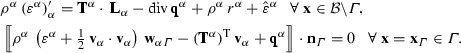
overall energy balance:
$$\begin{aligned} \begin{aligned}&\sum _\alpha \rho ^\alpha \,(\varepsilon ^\alpha )'_\alpha = \left( {\mathbf {{T}}}^{\mathrm{S}}_\mathrm{E} -p^{\mathrm{FR}}\,{\mathbf {{I}}}\right) \cdot \,{\mathbf {{L}}}_\mathrm{S}- n^{\mathrm{L}} p^{\mathrm{LR}}\,\mathrm{div}\,{\mathbf {{w}}}_\mathrm{L} - n^{\mathrm{G}} p^{\mathrm{GR}}\,\mathrm{div}\,{\mathbf {{w}}}_\mathrm{G}\\&\quad -\,\mathrm{div}\,{\mathbf {{q}}}- \hat{{\mathbf {{p}}}}^{\mathrm{L}} \cdot {\mathbf {{w}}}_\mathrm{L} - {\hat{{\mathbf {{p}}}}}^{\mathrm{G}} \cdot {\mathbf {{w}}}_\mathrm{G} - {\hat{\rho }}^{\mathrm{G}}\left[ \varepsilon ^{\mathrm{G}} -\varepsilon ^{\mathrm{L}} + \tfrac{1}{2}\,({\mathbf {{w}}}_\mathrm{G}\cdot {\mathbf {{w}}}_\mathrm{G} - {\mathbf {{w}}}_\mathrm{L}\cdot {\mathbf {{w}}}_\mathrm{L})\right] .\qquad \end{aligned} \end{aligned}$$(99)
The overall momentum balance is obtained by summing up the momentum balances (25)\(_3\) for \(\varphi ^{\mathrm{S}}, \varphi ^{\mathrm{G}}\) and \(\varphi ^{\mathrm{L}}\), where the partial stresses \({\mathbf {{T}}}^\alpha \) and the solid extra stresses \({\mathbf {{T}}}^{\mathrm{S}}_\mathrm{E} \approx \varvec{\sigma }^{\mathrm{S}}_\mathrm{E}\) are given by (26)\(_{2,\,3}\) and (45)\(_1, \rho \) is given by (5), and \(\sum _\alpha \hat{{\mathbf {{p}}}}^\alpha \) has been computed according to (23)\(_1\) and (24)\(_2\). The gas and liquid mass balances have been taken from (25)\(_2\), where they have been derived such that the material time derivatives of the gas and liquid phases have been expressed by the solid time derivative and additional terms according to the modified Eulerian setting of the fluid components. Under the assumption of negligible external heat supplies (\(r^\alpha =0\)), the overall energy balance has been taken from (69), where the same stresses have been included as in the momentum balance. The total heat influx has been defined by \({\mathbf {{q}}}= \sum _\alpha {\mathbf {{q}}}^\alpha \) with \({\mathbf {{q}}}^\alpha \) after (67) and (68), and \(\hat{{\mathbf {{p}}}}^{\mathrm{S}}\) and \(\hat{\rho }^\beta \) have been substituted with respect to (23)\(_1\) and (24)\(_{1,\,2}\). Furthermore, note in passing that the kinetic part of the phase-change energy, \(\hat{\rho }^{\mathrm{G}}\,[\, \tfrac{1}{2}\,({\mathbf {{w}}}_\mathrm{G}\cdot {\mathbf {{w}}}_\mathrm{G} - {\mathbf {{w}}}_\mathrm{L}\cdot {\mathbf {{w}}}_\mathrm{L})\,],\) can be neglected under creeping-flow conditions. Thus, this term is dropped in the weak form of the governing equations.
Given (99), one obtains the weak form of the governing equations by multiplication of (99)\(_{1-3}\) with the test functions \(\delta {\mathbf {{u}}}_\mathrm{S}, \delta p^{\mathrm{GR}}, \delta p^{\mathrm{LR}}\) and \(\delta \theta \) and integration over the volume \({{\mathcal {B}}}\) using the Gaussian integral theorem. Thus,
-
overall momentum balance:
$$\begin{aligned} {{\mathcal {G}}}_{{\mathbf {{u}}}_\mathrm{S}}= & {} \displaystyle \int \limits _{{{\mathcal {B}}}}\left( \varvec{\sigma }^{\mathrm{S}}_\mathrm{E}-p^{\mathrm{FR}}\,{\mathbf {{I}}}\right) \cdot \,\delta \varvec{\varepsilon }_\mathrm{S}\,\mathrm {d}v-\int \limits _{{{\mathcal {B}}}}\rho \,{\mathbf {{g}}}\cdot \delta {\mathbf {{u}}}_\mathrm{S}\,\mathrm {d}v+\int \limits _{{{\mathcal {B}}}}\hat{\rho }^{\mathrm{L}}\,({\mathbf {{w}}}_\mathrm{L}-{\mathbf {{w}}}_\mathrm{G})\,\cdot \,\delta {\mathbf {{u}}}_\mathrm{S}\,\mathrm {d}v\nonumber \\&\displaystyle -\int \limits _{{\mathcal {S}}}\left( \varvec{\sigma }_\mathrm{E}^{\mathrm{S}} - p^{\mathrm{FR}}\,{\mathbf {{I}}}\right) \,{\mathbf {{n}}}\,\cdot \,\delta {\mathbf {{u}}}_\mathrm{S}\,\mathrm {d}a=0, \end{aligned}$$(100) -
gas and liquid mass balances:
$$\begin{aligned} \begin{aligned} {{\mathcal {G}}}_{p^{\mathrm{GR}}}&= \displaystyle \int \limits _{{{\mathcal {B}}}}\left[ (\rho ^{\mathrm{G}})'_\mathrm{S}+\rho ^{\mathrm{G}}\,\mathrm{div}\,({\mathbf {{u}}}_\mathrm{S})'_\mathrm{S}\right] \,\delta p^{\mathrm{GR}}\,\mathrm {d}v- \int \limits _{{{\mathcal {B}}}}\rho ^{\mathrm{G}}\,{\mathbf {{w}}}_\mathrm{G}\cdot {\mathrm{grad}}\,\delta p^{\mathrm{GR}}\,\mathrm {d}v\,\\&\quad \displaystyle -\,\int \limits _{{{\mathcal {B}}}}\hat{\rho }^{\mathrm{G}}\,\delta p^{\mathrm{GR}}\,\mathrm {d}v+ \int \limits _{{\mathcal {S}}}\rho ^{\mathrm{G}}\,{\mathbf {{w}}}_\mathrm{G}\cdot {\mathbf {{n}}}\,\delta p^{\mathrm{GR}}\,\mathrm {d}a=0,\\ {{\mathcal {G}}}_{p^{\mathrm{LR}}}&= \displaystyle \int \limits _{{{\mathcal {B}}}}\left[ (\rho ^{\mathrm{L}})'_\mathrm{S}+\rho ^{\mathrm{L}}\,\mathrm{div}\,({\mathbf {{u}}}_\mathrm{S})'_\mathrm{S}\right] \,\delta p^{\mathrm{LR}}\,\mathrm {d}v- \int \limits _{{{\mathcal {B}}}}\rho ^{\mathrm{L}}\,{\mathbf {{w}}}_\mathrm{L}\cdot {\mathrm{grad}}\,\delta p^{\mathrm{LR}}\,\mathrm {d}v\,\\&\quad \displaystyle -\,\int \limits _{{{\mathcal {B}}}}\hat{\rho }^{\mathrm{L}}\,\delta p^{\mathrm{LR}}\mathrm {d}v+\int \limits _{{\mathcal {S}}}\rho ^{\mathrm{L}}\,{\mathbf {{w}}}_\mathrm{L}\cdot {\mathbf {{n}}}\,\delta p^{\mathrm{LR}}\,\mathrm {d}a=0, \end{aligned} \end{aligned}$$(101) -
overall energy balance:
$$\begin{aligned} {{\mathcal {G}}}_{\theta }= & {} \displaystyle \int \limits _{{{\mathcal {B}}}}\left\{ \,\rho ^{\mathrm{S}}\,(\varepsilon ^{\mathrm{S}})'_\mathrm{S} + \rho ^{\mathrm{L}}\,(\varepsilon ^{\mathrm{L}})'_\mathrm{L} + \rho ^{\mathrm{G}}\,(\varepsilon ^{\mathrm{G}})'_\mathrm{G} - (\varvec{\sigma }^{\mathrm{S}}_\mathrm{E} -p^{\mathrm{FR}}\,{\mathbf {{I}}}\,)\, \cdot \,(\varvec{\varepsilon }_\mathrm{S})^\prime _\mathrm{S}\,\right. \nonumber \\&\displaystyle +\left[ \,\,\hat{{\mathbf {{p}}}}^{\mathrm{L}}_\mathrm{E}\,- n^{\mathrm{L}} {\mathrm{grad}}\,p^{\mathrm{LR}} + p^{\mathrm{C}}\,(s^{\mathrm{G}}{\mathrm{grad}}\,n^{\mathrm{L}} - s^{\mathrm{L}} {\mathrm{grad}}\,n^{\mathrm{G}})\right] \,\cdot {\mathbf {{w}}}_\mathrm{L}\nonumber \\&\left. \displaystyle +\,(\,\hat{{\mathbf {{p}}}}^{\mathrm{G}}_\mathrm{E}\,- n^{\mathrm{G}} {\mathrm{grad}}\,p^{\mathrm{GR}})\,\cdot {\mathbf {{w}}}_\mathrm{G}\,+\,\hat{\rho }^{\mathrm{G}}\,(\varepsilon ^{\mathrm{G}}-\varepsilon ^{\mathrm{L}})\right\} \,\delta \theta \,\mathrm {d}v\,\nonumber \\&\displaystyle -\,\int \limits _{{{\mathcal {B}}}}({\mathbf {{q}}}+ n^{\mathrm{L}}\,p^{\mathrm{LR}}\,{\mathbf {{w}}}_\mathrm{L} + n^{\mathrm{G}}\,p^{\mathrm{GR}}\,{\mathbf {{w}}}_\mathrm{G})\cdot {\mathrm{grad}}\,\delta \theta \,\mathrm {d}v\, \nonumber \\&\displaystyle +\,\int \limits _{{\mathcal {S}}}({\mathbf {{q}}}+ n^{\mathrm{L}}\,p^{\mathrm{LR}}\,{\mathbf {{w}}}_\mathrm{L} +n^{\mathrm{G}}\,p^{\mathrm{GR}}\,{\mathbf {{w}}}_\mathrm{G})\cdot {\mathbf {{n}}}\,\delta \theta \,\mathrm {d}a=0. \end{aligned}$$(102)
In (100)–(102), the mass-transition term \(\hat{\rho }^{\mathrm{G}}\) is given by (76), (77), and (96), and \(\hat{{\mathbf {{p}}}}^{\mathrm{L}}_\mathrm{E}\) and \(\hat{{\mathbf {{p}}}}^{\mathrm{G}}_\mathrm{E}\) are given by (61). To set an example on how the temperature change comes into play, consider the terms
cf. (45)\(_1\) and (48), where, in the framework of small-strain approaches, \(\rho ^{\mathrm{S}} \approx \rho ^{\mathrm{S}}_{0\mathrm S}\) has been used. Further terms yielding \(\theta ^\prime _\beta = \theta ^\prime _\mathrm{S} + {\mathrm{grad}}\,\theta \cdot {\mathbf {{w}}}_\beta \) are included in \((\varepsilon ^\beta )^\prime _\beta \).
Given the above theoretical framework, the finite-element method (FEM) can be applied for the description and the illustration of numerical examples.
4.1 Condensation of \({\hbox {CO}}_2\) in a Deformable Porous Rock
In order to present the potential of the derived model, a two-dimensional example of a condensation process of \({\hbox {CO}}_2\) in a porous rock is simulated. Choosing this example, we are aware that considering the pure substance is somehow academic, since in real processes, such as \({\hbox {CO}}_2\) sequestration, the dissolution of \({\hbox {CO}}_2\) in saline water or brine, respectively, comes into play. Thus, our example might be considered as a state, where the injected \({\hbox {CO}}_2\) has completely displaced the saline water. Furthermore, the choice of \({\hbox {CO}}_2\) as the fluid under consideration results from the good knowledge of its thermodynamical behaviour and its low-temperature condensation point. Nevertheless, substituting \({\hbox {CO}}_2\) by water would also have been an option.
The initial state of the simulation domain of 10 m \(\times \) 10 m is composed of a thermoelastic porous solid filled with gaseous \({\hbox {CO}}_2\), which is guaranteed by an initial pore pressure of \(p^{\mathrm{FR}} = 4.0\) MPa. This value is also applied as Dirichlet boundary condition at the upper boundary in order to simulate an open boundary with connection to a surrounding environment also containing gaseous \({\hbox {CO}}_2\). Note in passing that \(s^{\mathrm{L}}=0\) at the upper boundary yields \(p^{\mathrm{FR}}=p^{\mathrm{GR}}\). The initial temperature in the whole system is set to 320 K, while the domain is horizontally confined at the left and right boundaries and vertically confined at the bottom, cf. Fig. 4. Then, the blue-coloured part of 2 m at the bottom is subjected to a temperature decrease from 320 K to 200 K over 500 s and held constant thereafter.

Simulation setup with constant pressure \(p^{\mathrm{FR}} = 4.0\) MPa at the top boundary and cooling from 320 K to 200 K at the blue part of the bottom boundary
For a realistic simulation, the solid parameters are resembling sandstone, which are included in Table 2. The thermodynamic parameters of CO\(_2\) in Table 2 have been taken from Abbott and Ness (1989), and fluid and solid parameters from Graf (2008) and Rutqvist et al. (2010). The effective fluid shear viscosities are determined as a function of temperature and effective density given by Fenghour et al. (1998) via
where the divergence of the viscosity around the critical point has been omitted, since we do not particularly describe the critical region here. However, for the formulation with respect to the critical region, the reader is referred to Vesovic et al. (1990).
In contrast to the original publication, (104)\(_1\) has been multiplied by \(10^{-6}\). This is due to the fact that Fenghour et al. have based their shear viscosity formulation on \(\upmu \)Pa s instead of Pa s, what is required in this publication. The coefficients \(a_i\) and \(d_{ij}\) included in (104)\(_{2,\,3}\) can be taken from Table 3, where all not listed \(d_{ij}\) are vanishing. Finally, note that \(m=4\) and \(n=8\).

Temperature \(\theta \)

Liquid mass production \(\hat{\rho }^{\mathrm{L}}\)
After discretisation, the strongly coupled system of partial differential equations given by (100)–(102) is solved monolithically with an unconditionally stable implicit time-integration scheme by use of the finite-element solver PANDAS.Footnote 2
The results of the simulation are depicted in Figs. 5, 6, 7, 8, 9, 10, and 11 and visualise the condensation of gaseous CO\(_2\) due to cooling. For each parameter, ten snapshots are presented, taken during the simulation at times at 0 h, 6.6 h, 12.2 h, 17.5 h, 22.5 h, 35.0 h, 47.0 h, 59.7 h, 72.2 h, and 82.8 h. The first set of pictures in Fig. 5 depicts the change in temperature due to the applied cooling condition. Figure 6 shows the liquid mass production \(\hat{\rho }^{\mathrm{L}}\), indicating the mass fraction of gaseous CO\(_2\) transferred to liquid CO\(_2\). It can be clearly observed that the mass transfer only appears in the transition zone, where both phases coexist. Note that this zone is indicated by the intermediate gas saturations \(s^{\mathrm{G}}\) given in Fig. 7. Thus, after complete transition of gaseous CO\(_2\) to liquid CO\(_2\), the mass production vanishes. The saturation plots, Figs. 7 and 8, also contain the gaseous and liquid seepage velocity vectors, respectively. It can be seen that gaseous CO\(_2\) is replenished from the open boundary and liquid CO\(_2\) is fanning-out along the transition zone. Finally, Figs. 9 and 10 show the partial pore densities \(\rho ^\beta _F:=s^\beta \rho ^{\beta \mathrm{R}}\) of the fluids depicting the transition from gaseous CO\(_2\) with a density of about 110 kg/m\(^3\) to liquid CO\(_2\) with a maximum density of 1200 kg/m\(^3\). Consequently, this increase in density causes a drop in pore pressure \(p^{\mathrm{FR}}\) that again affects the field of solid displacement vectors, represented in Fig. 11 by black arrows exhibiting a settlement zone around the cooling region.

Gas saturation \(s^{\mathrm{G}}\) and gaseous seepage-velocity vectors (black arrows)

Liquid saturation \(s^{\mathrm{L}}\) and liquid seepage-velocity vectors (black arrows)

Partial pore density \(\rho ^{\mathrm{G}}_F=s^{\mathrm{G}}\rho ^{\mathrm{GR}}\) of the gaseous phase

Partial pore density \(\rho ^{\mathrm{L}}_F=s^{\mathrm{L}}\rho ^{\mathrm{LR}}\) of the liquid phase

Pore pressure \(p^{\mathrm{FR}}\) together with the solid displacement vectors (black arrows)
5 Conclusion
In this article, the phase-transition process between liquid and gaseous phases of the same fluid substance has been simulated by the mass transfer over a phase-change interface. Apart from the direct momentum productions \(\hat{\mathbf{p}}^\beta \), the mass transfer couples the mass balance relations of the two fluid phases and influences the momentum and energy balances. To derive a thermodynamically consistent constitutive relation for the mass transfer, an immaterial, singular surface has been introduced representing the interface, across which jump conditions for the fluid constituents could be identified. Since the phase change did not affect the solid material, it has been assumed that the solid is continuous over the interface. The evaluation of the jump conditions of the balance equations led to a relation between the induced mechanical and non-mechanical power and the latent heat of vaporisation, thus describing the mass transfer over the interface. After averaging the mass-transfer term over the REV by introducing a so-called interfacial area, the averaged mass-transfer \(\hat{\rho }^{\mathrm{L}}=-\hat{\rho }^{\mathrm{G}}\) has been included in the global weak balance relations and, consequently, has been used for the simulation of gas–liquid phase transitions. Within a numerical example, the simulation of a condensation process of \({\hbox {CO}}_2\) in a thermoelastic porous rock was carried out showing reasonable results of the interaction between fluid thermodynamics, phase-change processes, fluid flow, and solid deformations with heat transfer.
The potential of the present model, which distinguishes from other more or less simple models, lies in the inclusion of solid deformations, compressible fluid phases based on the van der Waals equation, and an explicit constitutive relation of the interfacial mass production derived from the evaluation of balance relations at the interface, and not from additional assumptions.
6 Nomenclature
The notation in this article follows the conventions commonly used in modern tensor calculus, compare, for example, Ehlers (2015), while the symbols used in the porous-media context follow the established nomenclature by de Boer (2000) and Ehlers (2002, 2009, 1989).
6.1 Conventions
Kernel conventions | |
\((\,{{\varvec{\cdot }}}\,)\) | Place holder for arbitrary quantities |
\(s,t,\ldots \) or \(\sigma ,\tau ,\ldots \) | Scalars (tensors of order 0) |
\(\mathbf{s},\mathbf{t},\ldots \) or \({\varvec{\sigma }},{\varvec{\tau }},\ldots \) | Vectors (tensors of order 1) |
\(\mathbf{S},\mathbf{T},\ldots \) or \( {\varvec{\Psi }},\varvec{\Phi },\ldots \) | Tensors (tensors of order 2) |
| Higher-order tensors (tensors of order n) |
Index and suffix conventions | |
i, j, m, n | Indices as super- or subscripts range from 1 to N, where \(N=3\) indicates quantities of the usual three-dimensional (3D) space of our physical experience |
\((\,{{\varvec{\cdot }}}\,)_\alpha \) | Subscripts indicate kinematical quantities of a constituent within porous-media or mixture theories |
\((\,{{\varvec{\cdot }}}\,)^\alpha \) | Superscripts indicate the belonging of non-kinematical quantities to a constituent within mixture theories |
\((\,{{\varvec{\cdot }}}\,)'_\alpha \) | Material time derivative following the motion of a constituent \(\alpha \) with the solid and fluid constituents \(\alpha =\{\mathrm{S},\mathrm{L},\mathrm{G}\}\) |
\((\,{{\varvec{\cdot }}}\,)_{0\alpha }\) | Initial value of a non-kinematical quantity with respect to the referential configuration of a constituent |
\((\,{{\varvec{\cdot }}}\,)^{\mathrm{FM}},\ (\,{{\varvec{\cdot }}}\,)_{\mathrm{FM}}\) | Subscripts and superscripts “FM” indicate quantities of the fluid matter under consideration |
\((\,{{\varvec{\cdot }}}\,)_{\mathrm{m}},\ (\,{{\varvec{\cdot }}}\,)_{\theta }\) | Subscripts “m” and “\(\theta \)” indicate purely mechanical and purely thermal parts associated with thermoelastic solid kinematics |
\((\,{{\varvec{\cdot }}}\,)_\mathrm{crit}\) | Subscript “crit” indicates values at the critical point |
\({\hbox {d}}(\,{{\varvec{\cdot }}}\,)\) | Differential operator |
\(\partial (\,{{\varvec{\cdot }}}\,)\) | Partial derivative operator |
\(\delta (\,{{\varvec{\cdot }}}\,)\) | Test functions of the respective degrees of freedom |
\(\llbracket (\,{{\varvec{\cdot }}}\,)\rrbracket \) | Jump-related value on the discontinuity surface \(\varGamma \) |
\((\,{{\varvec{\cdot }}}\,)^+,(\,{{\varvec{\cdot }}}\,)^-\) | Quantity belonging to the pore gas (\({{\mathcal {B}}}^+={{\mathcal {B}}}^{\mathrm{G}}\)) or pore liquid (\({{\mathcal {B}}}^-={{\mathcal {B}}}^{\mathrm{L}}\)) |

6.2 Symbols
!h
Symbol | Unit | Description |
|---|---|---|
\(\alpha \) | Constituent identifier in super- and subscript, ı.e. \(\alpha =\{\mathrm{S},\mathrm{L},\mathrm{G}\}\) | |
\(\alpha ^{\mathrm{S}}\) | [ 1/K ] | Coefficient of thermal expansion of \(\varphi ^{\mathrm{S}}\) |
\(\beta \) | Fluid constituent identifier (here: \(\beta =\{\mathrm{L,G}\}\)) | |
\(\varGamma \) | Interface between the fluid phases | |
\(\varepsilon ^\alpha \) | [ J/kg ] | Mass-specific internal energy of \(\varphi ^\alpha \) |
\({\hat{\varepsilon }}^\alpha \) | [ J/m\(^3\) s ] | Volume-specific direct energy production of \(\varphi ^\alpha \) |
\(\zeta ^\alpha \) | [ J/K m\(^3\) s ] | Mass-specific Gibbs energy (enthalpy) of \(\varphi ^\alpha \) |
\(\varDelta \zeta _\mathrm{vap}\) | [ J/K m\(^3\) s ] | Mass-specific latent heat or enthalpy of evaporation |
\(\eta ^\alpha \) | [ J/K kg ] | Mass-specific entropy of \(\varphi ^\alpha \) |
\(\theta , \theta ^\alpha \) | [ K ] | Absolute temperature of \(\varphi \) and \(\varphi ^\alpha \) |
\(\theta _0, \varDelta \theta \) | [ K ] | Initial temperature and temperature variation |
\(\kappa \) | [ – ] | Exponent governing the deformation dependency of \(K^{\mathrm{S}}\) |
\(\lambda \) | [ – ] | Pore-size distribution index for Brooks & Corey law |
\(\lambda ^{\mathrm{S}}\) | [ N/m\(^2\) ] | 1st Lamé constant of \(\varphi ^{\mathrm{S}}\) |
\(\mu ^{\beta \mathrm{R}}\) | [ Pa s ] | Effective dynamic fluid viscosity of \(\varphi ^\beta \) |
\(\mu ^{\beta \mathrm{R}}_0, \varDelta \mu ^{\beta \mathrm{R}}\) | [ \(\upmu \)Pa s ] | Effective dynamic fluid viscosity of \(\varphi ^\beta \) at zero density and excess part |
\(\mu ^{\mathrm{S}}\) | [ N/m\(^2\) ] | 2nd Lamé constant of \(\varphi ^{\mathrm{S}}\) |
\(\pi \) | [ – ] | Circle constant |
\(\rho \) | [ kg/m\(^3\) ] | Density of the overall aggregate \(\varphi \) |
\(\rho ^\alpha , \rho ^{\alpha R}, \rho ^{\beta }_F\) | [ kg/m\(^3\) ] | Partial and effective (realistic) density of \(\varphi ^\alpha \) and partial pore density of \(\varphi ^\beta \) |
\(\hat{\rho }{}^\alpha \) | [kg/m\(^3\) s] | Volume-specific mass production of \(\varphi ^\alpha \) |
\(\hat{\varrho }{}^\beta _\varGamma \) | [ kg/m\(^2\) s ] | Area-specific interfacial mass transfer of \(\varphi ^\beta \) |
\(\sigma ^\alpha \) | Scalar-valued supply terms of mechanical quantities | |
\(\sigma ^*\) | [ – ] | Auxiliary term in the derivation of the shear viscosity |
\(\varphi , \varphi ^\alpha \) | Overall aggregate and constituent \(\alpha \) | |
\(\psi , \psi ^\alpha \) | [ J/kg ] | Mass-specific Helmholtz free energy of \(\varphi ^\alpha \) |
\(\varPsi ^\alpha \) | [ \(\cdot \)/m\(^3\) ] | Volume-specific densities of scalar mechanical quantities |
\(\hat{\varPsi }^\alpha \) | [ \(\cdot \)/m\(^3\) ] | Volume-specific productions of scalar mechanical quantities |
\(\varvec{\sigma }^\alpha \) | Vector-valued supply terms of mechanical quantities | |
\(\varvec{\phi }^\alpha \) | General vector-valued mechanical quantities | |
\(\varvec{\Psi }^\alpha \) | [ \(\cdot \)/m\(^3\) ] | Volume-specific densities of vectorial mechanical quantities |
\({\hat{\varvec{\Psi }}}^\alpha \) | [ \(\cdot \)/m\(^3\) ] | Volume-specific productions of vectorial mechanical quantities |
\(\varvec{\chi }_\alpha , \varvec{\chi }^{-1}_\alpha \) | Motion and inverse motion function of constituent \(\varphi ^\alpha \) | |
\(\varvec{\varepsilon }_\mathrm{S}\) | [ – ] | Linearised Green–Lagrangean solid strain tensor |
\(\varvec{\Phi }, \varvec{\Phi }^\alpha \) | General tensor-valued mechanical quantities | |
\(\varvec{\sigma }^{\mathrm{S}}_\mathrm{E}\) | [ N/m\(^2\) ] | Linearised 2nd Piola–Kirchhoff extra stress tensor of \(\varphi ^{\mathrm{S}}\) |
a | [ m\(^5\)/kg s\(^2\) ] | Cohesion pressure, constant of the van der Waals equation |
\(a_\varGamma \) | [1/m] | Volume-averaged interfacial area |
b | [ m\(^3\)/kg ] | Co-volume, constant of the van der Waals equation |
A, B, C | [ – ] | Empirical parameters of the Antoine equation |
\(A^{\mathrm{GL}}, A_\varGamma \) | [ m\(^2\) ] | Gas–liquid contact area in the volume-equivalent sphere, where \(A^{\mathrm{GL}}=A_\varGamma \) |
\(A^{\mathrm{SG}}, A^{\mathrm{SL}}\) | [ m\(^2\) ] | Solid–gas and solid–liquid contact areas of the volume-equivalent sphere |
\(A_\mathrm{REV}\) | [ m\(^2\) ] | Area of the REV |
\(a_i, b_i, d_{ij}\) | [ – ] | Coefficients for the calculation of the shear viscosity |
\({{\mathcal {B}}}, {{\mathcal {B}}}^\alpha \) | Body of the overall aggregate and partial body of constituent \(\varphi ^\alpha \) | |
\({{\mathcal {G}}}\) | Weak formulation of a governing equation related to a primary variable | |
\(c_\mathrm{V}^{\mathrm{S}},\, c^{\beta \mathrm{R}}_\mathrm{V}\) | [ J/kg K ] | Solid and effective fluid-specific heat capacities at constant volume |
\(d_{50}\) | [ m ] | Medial grain diameter of granular soil |
\(\mathrm {d}a_\varGamma , \mathrm {d}a_{\varGamma \,\mathrm{REV}}\) | [ m\(^2\) ] | Actual area element of the interface \(\varGamma \) and specific in the REV |
\(\mathrm {d}m^\alpha \) | [ kg ] | Local mass element of \(\varphi ^\alpha \) |
\(\mathrm {d}v^\alpha \) | [ m\(^3\) ] | Local volume element of \(\varphi ^\alpha \) |
\(\mathrm {d}v\) | [ m\(^3\) ] | Actual volume element of \(\varphi \) |
\({\hat{e}}^\alpha \) | [ J/m\(^3\) s ] | Volume-specific total energy production of \(\varphi ^\alpha \) |
f, k | Integration constants | |
\(h^D\) | [ m ] | Macroscopic capillary pressure head |
\(h^\beta \) | [ m ] | Filling height of volume-equivalent sphere of \(\varphi ^\beta \) |
\(H^\alpha \), \(H^{\alpha R}\) | [ W/K m ] | Isotropic partial and effective heat conduction of \(\varphi ^\alpha \) |
\(k^{\mathrm{S}}\) | [ N/m\(^2\) ] | Solid compression modulus |
\(k^\beta _\mathrm{r}\) | [ – ] | Relative permeability factor of \(\varphi ^\beta \) |
\(K^{\mathrm{S}}\) | [ m\(^2\) ] | Intrinsic (deformation-dependent) permeability of \(\varphi ^{\mathrm{S}}\) |
\(m^{\mathrm{S}}\) | [ N/K m\(^2\) ] | Solid compression modulus |
\(n^\alpha \) | [ – ] | Volume fraction of \(\varphi ^\alpha \) |
\(p^{\alpha R}, p_\mathrm{sat}\) | [ N/m\(^2\) ] | Effective pore pressure of \(\varphi ^\alpha \) and saturation pressure |
\(p^{\mathrm{C}}, p^D, p^{\mathrm{FR}}\) | [ N/m\(^2\) ] | Capillary pressure, bubbling or entry pressure and overall pore pressure |
\(P^\alpha \) | Material point of \(\varphi ^\alpha \) | |
\(r^\alpha \) | [ J/kg s ] | Mass-specific external heat supply of \(\varphi ^\alpha \) |
\({\bar{r}}^{\mathrm{F}}\) | [ m ] | Radius of the volume-equivalent sphere |
\({\bar{r}}^{\mathrm{S}}\) | [ m ] | Radius of a characteristic spherical solid particle |
\({\bar{R}}^\alpha \) | [ J/K ] | Specific gas constant of \(\varphi ^\alpha \) |
\(s^\alpha , s^{\mathrm{L}}_\mathrm{eff}, s^\beta _\mathrm{res}\) | [ – ] | Saturation of \(\varphi ^\beta \), effective liquid saturation, and residual saturations of \(\varphi ^\beta \) |
\({\mathcal {S}}, {\mathcal {S}}^\alpha \) | Surface of the overall aggregate and constituent \(\varphi ^\alpha \) | |
\(t, t_0\) | [ s ] | Actual time and reference time |
\(V, V^\alpha \) | [ m\(^3\) ] | Overall volume of \({{\mathcal {B}}}\) and partial volume of \({{\mathcal {B}}}^\alpha \) |
\({\mathbf {{b}}}, {\mathbf {{b}}}^\alpha \) | [ m/s\(^2\) ] | Mass-specific body force vector |
\(\mathrm {d}{\mathbf {{x}}}\) | [ m ] | Actual line element |
\(\mathrm {d}{\mathbf {{X}}}_\mathrm{S}\) | [ m ] | Reference line element of the solid |
\({\mathbf {{g}}}, g\) | [ m/s\(^2\) ] | Constant gravitation vector and scalar with \(|\,{\mathbf {{g}}}\,|=g=9.81\,\)m/s\(^2\) |
\({\mathbf {{n}}}\) | [ – ] | Outward-oriented unit surface normal vector |
\({\mathbf {{n}}}_\varGamma , {\mathbf {{n}}}_\varGamma ^\beta \) | [ – ] | Outward-oriented unit surface normal vector of the interface \(\varGamma \) |
\({\hat{{\mathbf {{p}}}}}^\alpha , \hat{{\mathbf {{p}}}}^\alpha _\mathrm{E}\) | [ N/m\(^3\) ] | Volume-specific direct and extra momentum production of \(\varphi ^\alpha \) |
\({\mathbf {{q}}}, {\mathbf {{q}}}^\alpha \) | [ J/m\(^2\) s ] | Heat influx vector of \(\varphi ^\alpha \) |
\(\hat{{\mathbf {{s}}}}^\alpha \) | [ N/m\(^3\) ] | Volume-specific total momentum production of \(\varphi ^\alpha \) |
\({\mathbf {{u}}}_\mathrm{S}\) | [ m ] | Solid displacement vector |
\({\mathbf {{v}}}_\alpha , {\mathbf {{v}}}_\varGamma \) | [ m/s ] | Velocity vector of \(\varphi ^\alpha , {\mathbf {{v}}}_\alpha ={\mathop {\mathbf x}\limits ^{\prime }_\alpha }\) and velocity vector of the interface \(\varGamma \) |
\({\mathbf {{w}}}_\beta \) | [ m/s ] | Fluid seepage velocity vector of \(\varphi ^\beta \) |
\({\mathbf {{w}}}_{\beta \varGamma }\) | [ m/s ] | Relative velocity vector of the fluid phases \(\varphi ^\beta \) with respect to \(\varGamma \) |
\({\mathbf {{x}}}\) | [ m ] | Actual position vector of \(\varphi \) |
\({\mathop {\mathbf x}\limits ^{\prime }_\alpha }, {\mathop {\mathbf x}\limits ^{\prime }_\varGamma }\) | [ m/s ] | Velocity vector of \(\varphi ^\alpha \) and velocity vector of the interface \(\varGamma \) |
\({\mathop {\mathbf x}\limits ^{\prime \prime }_\alpha }\) | [ m/s\(^2\) ] | Acceleration vector of \(\varphi ^\alpha \) |
\({\mathbf {{X}}}_\alpha \) | [ m ] | Reference position vector at time \(t_0\) |
| [ N/m\(^2\) ] | fourth-order elasticity tensor (elastic tangent) at the solid reference configuration |
\({\mathbf {{E}}}_\mathrm{S}\) | [ – ] | Green-Lagrangean solid strain tensor |
\({\mathbf {{F}}}_\mathrm{S}\) | [ – ] | solid deformation gradient |
\({\mathbf {{H}}}_\mathrm{S}\) | [ – ] | Solid displacement gradient |
\({\mathbf {{H}}}^\alpha \), \({\mathbf {{H}}}^{\alpha R}\) | [ W/K m ] | Partial and effective heat conduction tensor of \(\varphi ^\alpha \) |
\({\mathbf {{I}}}\) | [ – ] | Identity tensor (fundamental tensor of second order) |
\({\mathbf {{K}}}^\beta \) | [ m/s ] | Tensor of hydraulic conductivity of \(\varphi ^\beta \) |
\({\mathbf {{K}}}^\beta _\mathrm{r}\) | [ m/s ] | Tensor of relative permeability of \(\varphi ^\beta \) |
\({\mathbf {{K}}}^{\mathrm{S}}\) | [ \({\hbox {m}}^2\) ] | Intrinsic (deformation-dependent) permeability tensor of \(\varphi ^{\mathrm{S}}\) |
\({\mathbf {{L}}}_\alpha \) | [ 1/s ] | Spatial velocity gradient of \(\varphi ^\alpha \) |
\({\mathbf {{S}}}^{\mathrm{S}}_\mathrm{E}\) | [ N/m\(^2\) ] | 2nd Piola–Kirchhoff extra stress tensor of \(\varphi ^{\mathrm{S}}\) |
\({\mathbf {{T}}}^\alpha , {\mathbf {{T}}}^\alpha _\mathrm{E}\) | [ N/m\(^2\) ] | Cauchy or true stress tensor and extra stress tensor of \(\varphi ^\alpha \) |

Notes
The notion thermodynamically consistent expresses that the model is carefully elaborated with respect to the exploitation of the entropy inequality of the overall aggregate and that it only includes constitutive relations fulfiling the necessary requirements given by Truesdell’s principle of dissipation.
Porous media Adaptive Nonlinear finite-element solver based on Differential Algebraic Systems.
References
Abbott, M.M., van Ness, H.C.: Thermodynamics with Chemical Applications. McGraw-Hill, London (1989)
Alts, T., Hutter, K.: Continuum description of the dynamics and thermodynamics of phase boundaries between ice and water. Part I: surface balance laws and their interpretation in terms of three-dimensional balance laws averaged over the phase change boundary layer. J. Non-Equilib. Thermodyn. 13, 221–257 (1988)
Antoine, C.: Tensions des vapeurs; nouvelle relation entre les tensions et les températures. Comptes Rendus des Séances de l’Académie des Sciences 107, 681–684 (1888)
Bedeaux, D., Kjelstrup, S.: Transfer coefficients for evaporation. Phys. A 270, 413–426 (1999)
Biot, M.A.: General theory of three dimensional consolidation. J. Appl. Phys. 12, 155–164 (1941)
Bowen, R.M.: Theory of mixtures. In: Eringen, A.C. (ed.) Continuum Physics, III edn, pp. 1–127. Academic Press, New York (1976)
Bowen, R.M.: Incompressible porous media models by use of the theory of mixtures. Int. J. Eng. Sci. 18, 1129–1148 (1980)
Bowen, R.M.: Compressible porous media models by use of the theory of mixtures. Int. J. Eng. Sci. 20, 697–735 (1982)
Brooks, R.H., Corey, A.T.: Hydraulic Properties of Porous Media, Hydrology Papers, vol. 3. Colorado State University, Fort Collins (1964)
Chammari, A., Naon, B., Cherblanc, F., Bénet, J.C.: Water transport in soil with phase change. Mech. Model. Comput. Issues Civ. Eng. 23, 135–142 (2005)
de Boer, R.: Thermodynamics of phase transitions in porous media. Appl. Mech. Rev. 48, 613–622 (1995)
de Boer, R.: Theory of Porous Media. Springer, Berlin (2000)
de Boer, R., Bluhm, J.: Phase transitions in gas- and liquid-saturated porous solids. Transp. Porous Media 34, 249–267 (1999)
de Boer, R., Kowalski, S.J.: Thermodynamics of fluid-saturated porous media with a phase change. Acta Mech. 109, 167–189 (1995)
de Boer, R., Ehlers, W.: Theorie der Mehrkomponentenkontinua mit Anwendungen auf bodenmechanische Probleme. Forschungsberichte aus dem Fachbereich Bauwesen 40, Universität-GH-Essen (1986)
Ehlers, W.: Poröse Medien – ein kontinuumsmechanisches Modell auf der Basis der Mischungstheorie. Habilitation thesis, Report No. II-22 of the Institute of Applied Mechanics (CE), University of Stuttgart 2012. Reproduction of Forschungsberichte aus dem Fachbereich Bauwesen der Universität-GH-Essen 47, Essen (1989)
Ehlers, W.: Vector and Tensor Calculus. An Introduction. Lecture Notes, Institute of Applied Mechanics, University of Stuttgart 2015. http://www.mechbau.uni-stuttgart.de/ls2/Downloads/vektortensorskript_eng_ws1314.pdf
Ehlers, W.: Toward finite theories of liquid-saturated elasto-plastic porous media. Int. J. Plast. 7, 433–475 (1991)
Ehlers, W.: Grundlegende Konzepte in der Theorie Poröser Medien. Tech. Mech. 16, 63–76 (1996)
Ehlers, W.: Foundations of multiphasic and porous materials. In: Ehlers, W., Bluhm, J. (eds.) Porous Media: Theory, Experiments and Numerical Applications, pp. 3–86. Springer, Berlin (2002)
Ehlers, W., Graf, T., Ammann, M.: Deformation and localization analysis in partially saturated soil. Comput. Methods Appl. Mech. Eng. 193, 2885–2910 (2004)
Ehlers, W.: Challenges of porous media models in geo- and biomechanical engineering including electro-chemically active polymers and gels. Int. J. Adv. Eng. Sci. Appl. Math. 1, 1–24 (2009)
Ehlers, W., Graf, T.: Saturated elasto-plastic porous media under consideration of gaseous and liquid phase transitions. In: Schanz, T. (ed.) Theoretical and Numerical Unsaturated Soil Mechanics, Springer Proceedings in Physics 113, pp. 111–118. Springer, Berlin (2007)
Fenghour, A., Wakeham, W.A., Vesovic, V.: The viscosity of carbon dioxide. J. Phys. Chem. Ref. Data 27, 31–44 (1998)
Ghadiani, S.R.: A Multiphasic Continuum Mechanical Model for Design Investigations of an Effusion-Cooled Rocket Thrust Chamber. Dissertation thesis, Report No. II-13 of the Institute of Applied Mechanics (CE), University of Stuttgart (2005)
Graf, T.: Multiphase Flow Processes in Deformable Porous Media under Consideration of Fluid Phase Transitions. Dissertation thesis, Report No. II-17 of the Institute of Applied Mechanics (CE), University of Stuttgart (2008)
Gray, W.G.: General conservation equations for multi-phase systems: 4. Constitutive theory including phase change. Adv. Water Resour. 6, 130–140 (1983)
Hassanizadeh, S.M., Gray, W.G.: Mechanics and thermodynamics of multiphase flow in porous media including interphase boundaries. Adv. Water Resour. 13, 169–186 (1990)
Huang, H., Lin, P., Zhou, W.: Moisture transport and diffusive instability during bread baking. SIAM J. Appl. Math. 68, 222–238 (2006)
Jamet, D.: Diffuse interface models in fluid mechanics. GdR CNRS documentation, cf. http://pmc.polytechnique.fr/mp/GDR/docu/Jamet.pdf (2014)
Joekar-Niasar, V., Hassanizadeh, S.M., Leijnse, A.: Insights into the relationships among capillary pressure, saturation, interfacial area and relative permeability using pore-network modelling. Transp. Porous Media 74, 201–219 (2008)
Juric, D., Tryggvason, G.: Computations of boiling flows. Int. J. Multiph. Flow 24, 387–410 (1998)
Kowalski, S.J.: Toward a thermodynamics and mechanics of drying processes. Chem. Eng. Sci. 55, 1289–1304 (2000)
Lozano, A.-L., Cherblanc, F., Cousin, B., Bénet, J.-C.: Experimental study and modelling of water phase change kinetics in soils. Eur. J. Soil Sci. 59, 939–949 (2008)
Lozano, A.-L., Cherblanc, F., Bénet, J.-C.: Water evaporation versus condensation in a hygroscopic soil. Transp. Porous Media 80, 209–222 (2009)
Lu, S.C.H., Pister, K.S.: Decomposition of deformation and representation of the free energy function for isotropic thermoelastic solids. Int. J. Solids Struct. 11, 927–934 (1975)
Lykov, A.V.: On systems of differential equations for heat and mass transfer in capillary porous bodies. J. Eng. Phys. 26, 11–17 (1974)
Markert, B.: A constitutive approach to 3-d nonlinear fluid flow through finite deformable porous continua. Transp. Porous Media 70, 427–450 (2007)
Morland, L.W., Gray, J.M.N.T.: Phase change interactions and singular fronts. Contin. Mech. Thermodyn. 7, 387–414 (1995)
Morland, L.W., Sellers, S.: Multiphase mixtures and singular surfaces. Int. J. Non-Linear Mech. 36, 131–146 (2001)
Niessner, J., Hassanizadeh, S.M.: A model for two-phase flow in porous media including fluid–fluid interfacial area. Water Resour. Res. 44, 1–10 (2008)
Niessner, J., Hassanizadeh, S.M.: Modeling kinetic interphase mass transfer for two-phase flow in porous media including fluid–fluid interfacial area. Transp. Porous Media 80, 329–344 (2009a)
Niessner, J., Hassanizadeh, S.M.: Non-equilibrium interphase heat and mass transfer during two-phase flow in porous media—theoretical considerations and modeling. Adv. Water Resour. 32, 1756–1766 (2009b)
Ruiz, T., Bénet, J.-C.: Phase change in a heterogeneous medium: comparison between the vaporisation of water and heptane in an unsaturated soil at two temperatures. Transp. Porous Media 44, 337–353 (2001)
Rutqvist, J., Vasco, D.W., Myer, L.: Coupled reservoir-geomechanical analysis of \({{\text{ CO }}_2}\) injection and ground deformations at In Salah, Algeria. Int. J. Greenhouse Gas Control 4, 225–230 (2010)
Sahimi, M.: Flow and Transport in Porous Media and Fractured Rock: From Classical Methods to Modern Approaches, Second, Revised and Enlarged edn. Wiley-VCH, Weinheim (2011)
Schrefler, B.A., Zhan, X.: A fully coupled model for water flow and air flow in deformable porous media. Water Resour. Res. 29, 155–167 (1993)
Schrefler, B.A., Scotta, R.: A fully coupled model for two-pase flow in deformable porous media. Comput. Methods Appl. Mech. Eng. 190, 3223–3246 (2001)
Silhavy, M.: The Mechanics and Thermodynamics of Continuous Media. Springer, Berlin (1997)
Tanguy, S., Ménard, T., Berlemont, A.: A level set method for vaporizing two-phase flow. J. Comput. Phys. 221, 837–853 (2007)
Truesdell, C.: Rational Thermodynamics, 2nd edn. Springer, New York (1984)
van der Waals, J.D.: Over de Continuiteit van den Gas- en Vloeistoftoestand. Academisch proefschrift, Sijthoff, Leiden (1873)
van Genuchten, M.T.: A closed-form equation for predicting the hydraulic conductivity of unsaturated soils. Soil Sci. Soc. Am. J. 44, 892–898 (1980)
Vesovic, V., Wakeham, W.A., Olchowy, G.A., Sengers, J.V., Watson, J.T.R., Millat, J.: The transport properties of carbon dioxide. J. Phys. Chem. Ref. Data 19, 763–808 (1990)
Wang, Y., Oberlack, M.: A thermodynamic model of multiphase flows with moving interfaces and contact line. Contin. Mech. Thermodyn. 23, 409–433 (2011)
Whitaker, S.: Simultaneous heat, mass, and momentum transfer in porous media: a theory of drying. Adv. Heat Transf. 13, 119–203 (1977)
Wieners, C., Ammann, M., Graf, T., Ehlers, W.: Parallel Krylov methods and the application to 3-d simulations of a triphasic porous media model in soil mechanics. Comput. Mech. 36, 409–420 (2005)
Acknowledgments
The authors would like to thank the German Research Foundation (DFG) for financial support of this work within the International Graduate School for Non-linearities and Upscaling in Porous Media (NUPUS) at the University of Stuttgart.
Author information
Authors and Affiliations
Corresponding author
Rights and permissions
Open Access This article is distributed under the terms of the Creative Commons Attribution 4.0 International License (http://creativecommons.org/licenses/by/4.0/), which permits unrestricted use, distribution, and reproduction in any medium, provided you give appropriate credit to the original author(s) and the source, provide a link to the Creative Commons license, and indicate if changes were made.
About this article

Cite this article
Ehlers, W., Häberle, K. Interfacial Mass Transfer During Gas–Liquid Phase Change in Deformable Porous Media with Heat Transfer. Transp Porous Med 114, 525–556 (2016). https://doi.org/10.1007/s11242-016-0674-2
Received:
Accepted:
Published:
Issue Date:
DOI: https://doi.org/10.1007/s11242-016-0674-2