
Abstract
In this paper, symmetries and symmetry reduction of two higher-dimensional nonlinear evolution equations (NLEEs) are obtained by Lie group method. These NLEEs play an important role in nonlinear sciences. We derive exact solutions to these NLEEs via the \(\exp(-\phi (z))\)-expansion method and complex method. Five types of explicit function solutions are constructed, which are rational, exponential, trigonometric, hyperbolic and elliptic function solutions of the variables in the considered equations.
1 Introduction
In 1998, Yu et al. [1] extended the Bogoyavlenskii Schiff equation
to the \((3+1)\)-dimensional NLEE
Setting \(u:=u_{x}\), equation (2) is changed into the \((3+1)\)-dimensional potential Yu-Toda-Sasa-Fukuyama (YTSF) equation
The generalized \((3+1)\)-dimensional Zakharov-Kuznetsov (gZK) equation is given by
Here \(a_{i}\) (\(i=1,2,\ldots,6\)) are arbitrary constants.
We note that equation (4) includes many famous NLEEs as its special cases. For instance, if \(a_{1}=a_{3}=a_{4}=a_{6}=0\), then equation (4) is the Korteweg-de Vries equation [2, 3]. If \(a_{2}=a_{4}=a_{5}=0\), then equation (4) is the \((2+1)\) dimensional ZK-MEW equation [4]. If \(a_{3}=a_{4}=a_{6}=0\), then equation (4) is the Gardner equation [5]. If \(a_{4}=a_{5}=a_{6}=0\), then equation (4) is the modified Zakharov-Kuznetsov equation [6].
In recent years, it has aroused widespread interest in the study of NLEEs [7–13]. Equations (3) and (4) are very meaningful higher-dimensional NLEEs which can describe many dynamic processes and important phenomena in engineering and physics. The YTSF equation is a mostly used model for investigating the dynamics of solitons and nonlinear waves in fluid dynamics, plasma physics and weakly dispersive media [13]. Zakharov and Kuznetsov [14] proposed the ZK equation to describe nonlinear ion-acoustic waves in a plasma comprised of cold ions and hot isothermal electrons in the presence of a uniform magnetic field. Many physical phenomena, in the purely dispersive limit, are governed by this type of equation, such as the long waves on a thin liquid film [15], the Rossby waves in a rotating atmosphere [16], and the isolated vortex of drift waves in a three-dimensional plasma [17]. The gZK equation is of a generalized setting of ZK equation. Seeking exact solutions of NLEEs is an interesting and significant subject. Over the past few years, many powerful methods for constructing the solutions of NLEEs have been used, for instance, the Bäcklund transform method [18], direct algebraic method [19], modified simple equation method [20], Lie group method [21, 22], \(\exp(-\phi(z))\)-expansion method [8, 9, 23, 24], and so on. Recently, Yuan et al. [25–27] introduced the complex method to find the exact solutions of NLEEs in mathematical physics. In this paper, we study symmetries, symmetry reduction of the two higher-dimensional NLEEs, and then we obtain their exact solutions via the \(\exp(-\phi(z))\)-expansion method and complex method.
2 Description of the methods
2.1 Description of the \(\exp(-\phi(z))\)-expansion method
Suppose that a nonlinear partial differential equation (PDE) is given by
where P is a polynomial of an unknown function \(u(x,y,t)\) and its derivatives in which nonlinear terms and highest order derivatives are involved. The main steps of this method are given in the following.
Step 1. Substituting the traveling wave transform
into equation (5) converts it to the following ordinary differential equation (ODE):
in which F is a polynomial of \(w(z)\) and its derivatives, while \(':=\frac{d}{dz}\).
Step 2. Assume that equation (6) has the following traveling wave solution:
where \(C_{j}\) (\(0\leq j\leq n\)) are constants to be determined, such that \(C_{j}\neq0\) and \(\phi=\phi(z)\) satisfies the ODE as follows:
Equation (8) has the following solutions.
When \(\delta^{2}-4\mu>0\), \(\mu\neq0\),
When \(\delta^{2}-4\mu<0\), \(\mu\neq0\),
When \(\delta^{2}-4\mu>0\), \(\mu=0\), \(\delta\neq0\),
When \(\delta^{2}-4\mu=0\), \(\mu\neq0\), \(\delta\neq0\),
When \(\delta^{2}-4\mu=0\), \(\mu=0\), \(\delta=0\),
Here \(C_{n}\neq0\), δ, μ are constants that will be determined later and c is an arbitrary constant. We take the homogeneous balance between nonlinear terms and highest order derivatives of equation (6) to determine the positive integer n.
Step 3. Substituting equation (7) into equation (6) and accounting the function \(\exp(-\phi(z))\), we obtain a polynomial of \(\exp(-\phi(z))\). Equating all the coefficients of the same power of \(\exp(-\phi(z))\) to zero yields a set of algebraic equations. By solving the algebraic equations, we get the values of \(C_{n}\neq0\), δ, μ, and then we substitute them into equation (7) along with equations (9)-(15) to complete the determination of the solutions of equation (5).
2.2 Description of the complex method
Let \(m\in{\mathbb {N}}^{*}:=\{1, 2, 3,\ldots\}\), \(r_{j}\in{\mathbb {N}}={\mathbb {N}}^{*}\cup\{0\}\), \(j=0, 1, \ldots, m\), \(r=(r_{0}, r_{1},\ldots, r_{m})\), and
then \(d(r):=\sum_{j=0}^{m}r_{j}\) is the degree of \(K_{r}[w]\). Let the differential polynomial be defined by
where J is a finite index set, and \(a_{r}\) are constants, then \(\deg F(w,w',\ldots,w^{(m)}):=\max_{r\in J}\{d(r)\}\) is the degree of \(F(w,w',\ldots,w^{(m)})\).
Consider the following differential equation:
where \(n\in{\mathbb {N}}^{*}\), \(c\neq0\), d are constants.
Set \(p, q\in{\mathbb {N}}^{*}\), and the meromorphic solutions w of equation (16) have at least one pole. If equation (16) has exactly p distinct meromorphic solutions, and their multiplicity of the pole at \(z=0\) is q, then equation (16) is said to satisfy the \(\langle p,q \rangle\) condition. It might not be easy to show that the \(\langle p,q \rangle\) condition of equation (16) holds, so we need the weak \(\langle p,q \rangle \) condition as follows.
Inserting the Laurent series
into equation (16), we can determine exactly p different Laurent singular parts:
then equation (16) is said to satisfy the weak \(\langle p,q \rangle\) condition.
Given two complex numbers \(\nu_{1}\), \(\nu_{2}\) such that \(\operatorname{Im} \frac{\nu_{1}}{\nu_{2}} >0\), and let L be the discrete subset \(L[2\nu_{1}, 2\nu_{2}]:=\{\nu\mid \nu=2a_{1}\nu_{1}+2a_{2}\nu_{2}, a_{1},a_{2}\in\mathbb {Z}\}\), and L is isomorphic to \({\mathbb {Z}}\times{\mathbb {Z}}\). Let the discriminant \(\varDelta =\varDelta (b_{1},b_{2}):=b_{1}^{3}-27b_{2}^{2}\) and
A meromorphic function \(\wp(z):=\wp(z,g_{2},g_{3})\) with double periods \(2\nu_{1}\), \(2\nu_{2}\), which satisfies the following equation:
in which \(g_{2}=60l_{4}\), \(g_{3}=140l_{6}\), and \(\varDelta (g_{2},g_{3})\neq0\), is called the Weierstrass elliptic function and satisfies an addition formula [28] as follows:
If a meromorphic function g is a rational function of z, or a rational function of \(e^{\alpha z}\), \(\alpha\in{\mathbb {C}}\), or an elliptic function, then we say that g belongs to the class W.
In 2009, Eremenko et al. [29] studied the mth-order Briot-Bouquet equation (BBEq)
where \(F_{j}(w)\) are constant coefficients polynomials, \(m\in{\mathbb {N}}^{*}\). For the mth-order BBEq, we have the following lemma.
Lemma 2.1
Let \(m, n, p, h\in{\mathbb {N}}^{*}\), \(\deg F(w,w^{(m)}) < n \), and a mth-order BBEq
satisfies the weak \(\langle p,q \rangle\) condition, then the meromorphic solutions \(w\in W\). Supposing for some values of the parameters the solution w exists, then any other meromorphic solutions will be one parameter family \(w(z+z_{0})\), \(z_{0}\in{\mathbb {C}}\). In addition, every elliptic solution w with a pole at \(z=0\) is expressed as
where \(\beta_{-ij}\) are determined by (17), \(\sum_{i=1}^{h}\beta _{-i1}=0\) and \(D_{i}^{2}=4B_{i}^{3}-g_{2}B_{i}-g_{3}\).
Every rational function solution \(w:=R(z)\) is expressed as
which has h (≤p) distinct poles of multiplicity q.
Every simply periodic solution \(w:=R(\vartheta)\) is a rational function of \(\vartheta=e^{\alpha z}\) (\(\alpha\in{\mathbb {C}}\)), and is expressed as
which has h (≤p) distinct poles of multiplicity q.
By the above definitions and lemma, we now present the complex method.
Step 1. Insert the transformation \(T: u(x,y,t)\rightarrow w(z)\) defined by \((x,y,t)\rightarrow z \) into a given PDE to yield a nonlinear ODE.
Step 2. Insert (17) into the ODE to determine whether the weak \(\langle p,q \rangle\) condition holds.
Step 3. Insert the indeterminate solutions introduced in Lemma 2.1 into the ODE, and then get meromorphic solutions of the ODE with a pole at \(z=0\).
Step 4. Obtain meromorphic solutions \(w(z-z_{0})\) by Lemma 2.1 and the addition formula.
Step 5. Inserting the inverse transformation \(T^{-1}\) into the meromorphic solutions, we get the exact solutions for the original PDE.
3 Symmetries and symmetry reduction
3.1 Symmetries
In order to find the symmetry \(\sigma=\sigma(x,y,s,t,u)\) of equation (4), we set
where u is the solution of equation (4), a, b, c, d, e, f are unknown functions of real variables x, y, s, t. According to Lie group analysis [21, 22], σ satisfies
Substituting equation (21) into equation (22), we have a new differential equation, where
By equation (21), equation (22) and equation (23), we have
where \(c_{i}\) (\(i=2,3,4,5\)) are real constants. Substituting equations (24) into equation (21), we achieve the symmetry of the gZK equation,
In order to find the symmetry \(\sigma=\sigma(x,y,s,t,u)\) of equation (3), we set
Here u is the solution of equation (3), a, b, c, d, e, f are unknown functions of real variables x, y, s, t. According to Lie group analysis, σ satisfies
Substituting equation (26) into equation (27), we have a new differential equation, where
By equation (26), equation (27) and equation (28), we have
where \(c_{i}\) (\(i=1,2,\ldots,5\)) are real constants, \(\rho(t)\), \(\tau(t)\), \(\psi(t) \) are arbitrary real functions of t. Substituting equations (29) into equation (26), we achieved the symmetry of YTSF equation
3.2 Symmetry reduction
By solving the characteristic equation (25) of σ
we find different symmetry reduced equations. Without loss of generality, we have two reduced equations as follows.
Setting \(c_{1}=c_{3}=c_{4}=c_{5}=0\), \(c_{2}=1\), we have the first similarity solution of equation (4)
where \(\xi=x+t\), \(\eta=\frac{y^{2}}{2a_{3}}+\frac{s^{2}}{2a_{4}}\). Substituting equation (32) into equation (4), we have the first symmetry reduced equation of equation (4)
Setting \(c_{1}=c_{2}=0\), \(c_{3}=c_{4}=c_{5}=1\), solving \(\sigma=0\), we have the second similarity solution of equation (4)
where \(\xi=x+y\), \(\eta=s\). Substituting equation (34) into equation (4), we have the second symmetry reduced equation of equation (4)
By solving the characteristic equation (30) of σ
we obtain symmetry reduction of equation (3). Without loss of generality, we have two reduced equations as follows.
Setting \(c_{1}=c_{3}=c_{4}=0\), \(c_{2}=c_{5}=1\), \(\rho(t)=1\), solving \(\sigma=0\), we have the first similarity solution of equation (3)
where \(\xi=x-t\), \(\eta=s-t\). Substituting equation (36) into equation (3), we have the first symmetry reduced equation of equation (3)
Setting \(c_{1}=c_{2}=c_{3}=c_{5}=0\), \(c_{4}=1\), \(\rho(t)=\tau(t)=0\), solving \(\sigma=0\), we have the second similarity solution of equation (3)
Substituting equation (38) into equation (3), we have the second symmetry reduced equation of equation (3)
4 Exact solutions
4.1 Exact solutions of gZK equation via the \(\exp(-\phi (z))\)-expansion method
Substituting the traveling wave transform
into equation (33), then integrating it with respect to z, we obtain
where γ is the integration constant which can be determined later.
Taking the homogeneous balance between \(w''\) and \(w^{3}\) in equation (39) yields
where \(C_{1}\neq0\), \(C_{0}\) are constants to be determined, whereas δ and μ are arbitrary constants.
Substitute w, \(w^{2}\), \(w^{3}\), \(w''\) into equation (39) and equate the coefficients of \(\exp(-\phi(z))\) to zero, then
Solving the above algebraic equations, we obtain
where μ and δ are arbitrary constants.
Substituting equations (41) into equation (40) yields
We apply equation (9) to equation (15) into equation (42), respectively, to get traveling wave solutions of the gZK equation as follows.
When \(\delta^{2}-4\mu>0\), \(\mu\neq0\),
When \(\delta^{2}-4\mu<0\), \(\mu\neq0\),
When \(\delta^{2}-4\mu>0\), \(\mu=0\), \(\delta\neq0\),
When \(\delta^{2}-4\mu=0\), \(\mu\neq0\), \(\delta\neq0\),
When \(\delta^{2}-4\mu=0\), \(\mu=0\), \(\delta=0\),
4.2 Exact solutions of gZK equation via the complex method
Inserting (17) into equation (39) we have \(p=2\), \(q=1\), \(\beta_{{-1}}=\pm\sqrt{\frac{-6 ( a_{2} {k}^{2}+a_{3} {k}^{2}+2 {l}^{2} )}{a_{1}}}\), \(\beta_{{0}}=-\frac{a_{5}}{2a_{1}}\), \(\beta_{{1}}=-\frac{a_{5}^{2}}{24a_{1}^{2}}\sqrt {\frac{-6a_{1}}{ a_{2} {k}^{2}+a_{3} {k}^{2}+2 {l}^{2}}}\), \(\beta _{{2}}=-\frac{12a_{1}^{2}\gamma-a_{5}^{3}+6a_{1}a_{5}}{48a_{1}^{2}( a_{2} {k}^{2}+a_{3} {k}^{2}+2 {l}^{2})}\) and \(\beta_{3}\) is an arbitrary constant.
Therefore, equation (39) is a second order BBEq and satisfies the weak \(\langle2,1 \rangle\) condition. Hence, by Lemma 2.1, we see that meromorphic solutions of equation (39) belong to W. We will show meromorphic solutions of equation (39) in the following.
By (19), we infer that the indeterminate rational solutions of equation (39) are
with a pole at \(z=0\).
Substituting \(R_{1}(z)\) into equation (39), we have
where \(a_{5}^{2}=4a_{1}\) and \(9a_{1}\gamma^{2}=1\);
where \(k=\sqrt{\frac{4a_{1}z_{1}^{2}-a_{5}^{2}z_{1}^{2}-48l^{2}a_{1}}{24a_{1}(a_{2}+a_{3})}}\) and \(\gamma=(a_{5}^{3}-6a_{1}a_{5}+(a_{5}^{2}-4a_{1})^{\frac{3}{3}})z_{1}^{3}\).
So the rational solutions of equation (39) are
and
where \(z_{0}\in{\mathbb {C}}\), \(z_{1}\neq0\). \(a_{5}^{2}=4a_{1}\), \(9a_{1}\gamma^{2}=1\) in the former case, or \(k=\sqrt{\frac {4a_{1}z_{1}^{2}-a_{5}^{2}z_{1}^{2}-48l^{2}a_{1}}{24a_{1}(a_{2}+a_{3})}}\), \(\gamma =(a_{5}^{3}-6a_{1}a_{5}+(a_{5}^{2}-4a_{1})^{\frac{3}{3}})z_{1}^{3}\) in the latter case.
To obtain simply periodic solutions, let \(\vartheta=e^{\alpha z}\), and substitute \(w=R(\vartheta)\) into equation (39), then
Substituting
into equation (43), we obtain
and
where \(\gamma = \frac{a_{5}(a_{5}^{2}-6a_{1})}{12a_{1}^{2}}\), \(l = \frac{1}{2\alpha} \sqrt{ \frac{4a_{1}-a_{5}^{2}-2a_{1}k^{2}\alpha ^{2}(a_{2}+a_{3})}{a_{1}}}\) in the former case, or \(\gamma = \frac{\sqrt {3}z_{1}(z_{1}+1)(4a_{1}-a_{5}^{2})^{\frac{3}{2}}}{(z_{1}^{2}+10z_{1}+1)^{\frac {3}{2}}a_{1}^{2}} +\frac{a_{5}(a_{5}^{2}-6a_{1})}{12a_{1}^{2}}\), \(k=-\sqrt{\frac{(4a_{1}-a_{5}^{2}-4a_{1}l^{2}\alpha ^{2})(z_{1}^{2}+1)+2(a_{5}^{2}-4a_{1}-20a_{1}l^{2}\alpha ^{2})z_{1}}{2a_{1}(z_{1}^{2}+10z_{1}+1)(a_{2}+a_{3})\alpha^{2}}}\) in the latter case.
Inserting \(\vartheta=e^{\alpha z}\) into equation (44) and equation (45), we can get simply periodic solutions to equation (39) with a pole at \(z=0\),
where \(\gamma = \frac{a_{5}(a_{5}^{2}-6a_{1})}{12a_{1}^{2}}\), \(l = \frac{1}{2\alpha} \sqrt{ \frac{4a_{1}-a_{5}^{2}-2a_{1}k^{2}\alpha ^{2}(a_{2}+a_{3})}{a_{1}}}\) in the former case, or \(\gamma = \frac{\sqrt {3}z_{1} (z_{1}+1)(4a_{1}-a_{5}^{2})^{\frac{3}{2}}}{(z_{1}^{2}+10z_{1}+1)^{\frac {3}{2}}a_{1}^{2}}+\frac{a_{5}(a_{5}^{2}-6a_{1})}{12a_{1}^{2}}\), \(k=-\sqrt{\frac{(4a_{1}-a_{5}^{2}-4a_{1}l^{2}\alpha ^{2})(z_{1}^{2}+1)+2(a_{5}^{2}-4a_{1}-20a_{1}l^{2}\alpha ^{2})z_{1}}{2a_{1}(z_{1}^{2}+10z_{1}+1)(a_{2}+a_{3})\alpha^{2}}}\) in the latter case.
So simply periodic solutions of equation (39) are
and
where \(z_{0}\in{\mathbb {C}}\), \(z_{1}\neq0\). \(l=\frac{1}{2\alpha}\sqrt{\frac {4a_{1}-a_{5}^{2}-2a_{1}k^{2}\alpha^{2}(a_{2}+a_{3})}{a_{1}}}\), \(\gamma=\frac {a_{5}(a_{5}^{2}-6a_{1})}{12a_{1}^{2}}\) in the former case, or \(k=-\sqrt{\frac{(4a_{1}-a_{5}^{2}-4a_{1}l^{2}\alpha ^{2})(z_{1}^{2}+1)+2(a_{5}^{2}-4a_{1}-20a_{1}l^{2}\alpha ^{2})z_{1}}{2a_{1}(z_{1}^{2}+10z_{1}+1)(a_{2}+a_{3})\alpha^{2}}}\), \(\gamma=\frac{\sqrt {3}z_{1}(z_{1}+1)(4a_{1}-a_{5}^{2})^{\frac{3}{2}}}{(z_{1}^{2}+10z_{1}+1)^{\frac {3}{2}}a_{1}^{2}}+\frac{a_{5}(a_{5}^{2}-6a_{1})}{12a_{1}^{2}}\) in the latter case.
From (18), we have the indeterminate relations for the elliptic solutions of equation (39) with a pole at \(z=0\),
where \(D_{1}^{2}=4B_{1}^{3}-g_{2}B_{1}-g_{3}\). Considering the results obtained above, we infer that \(\beta_{0}=-\frac{a_{5}}{2a_{1}}\), \(g_{3}=0\), \(D_{1}=B_{1}=0\). So we obtain
where \(g_{3}=0\).
Thus, the elliptic function solutions of equation (39) are
where \(z_{0}\in{\mathbb {C}}\), \(g_{3}=0\), \(g_{2}\) is arbitrary. Applying the addition formula, we can rewrite it as
where \(g_{3}=0\), \(F^{2}=4E^{3}-g_{2}E\), E and \(g_{2}\) are arbitrary.
4.3 Exact solutions of YTSF equation via the \(\exp(-\phi (z))\)-expansion method
Substituting the traveling wave transform
into equation (37), then integrating it with respect to z, we obtain
where γ is the integration constant which can be determine later.
Setting \(w=v'\), equation (46) becomes
Taking the homogeneous balance between \(w''\) and \(w^{2}\) in equation (47) yields
where \(C_{2}\neq0\), \(C_{i}\) (\(i=0,1,2\)) are constants to be determined, whereas δ and μ are arbitrary constants.
Substitute w, \(w^{2}\), \(w''\) into equation (47) and equate the coefficients of \(\exp(-\phi(z))\) to zero, then
Solving the above algebraic equations, we obtain
where μ and δ are arbitrary constants.
Substituting equations (49) into equation (48), yields
We apply equation (9) to equation (15) into equation (50), respectively, to get traveling wave solutions of the YTSF equation as follows.
When \(\delta^{2}-4\mu>0\), \(\mu\neq0\),
When \(\delta^{2}-4\mu<0\), \(\mu\neq0\),
When \(\delta^{2}-4\mu>0\), \(\mu=0\), \(\delta\neq0\),
When \(\delta^{2}-4\mu=0\), \(\mu\neq0\), \(\delta\neq0\),
When \(\delta^{2}-4\mu=0\), \(\mu=0\), \(\delta=0\),
4.4 Exact solutions of YTSF equation via the complex method
Inserting (17) into equation (47) we have \(p=1\), \(q=2\), \(\beta_{{-2}}=-2k\), \(\beta_{{-1}}=0\), \(\beta_{{0}}=-\frac {4lk+4k^{2}+3r^{2}}{6k^{2}l}\), \(\beta_{{1}}=0\), \(\beta_{{2}}=-\frac {16k^{4}+32lk^{3}+(16l^{2}-12l\gamma+24r^{2})k^{2}+24lkr^{2}+9r^{4}}{120k^{5}l^{2}}\), and \(\beta_{3}\) is an arbitrary constant.
Therefore, equation (47) is a second order BBEq and satisfies the weak \(\langle1,2 \rangle\) condition. Hence, by Lemma 2.1, we see that meromorphic solutions of equation (47) belong to W. We will show meromorphic solutions of equation (47) in the following.
By (19), we deduce the indeterminacy rational solutions of equation (47) are
with a pole at \(z=0\).
Substituting \(R_{1}(z)\) into equation (47), we get the following form:
where \(\gamma=\frac{16k^{4}+32lk^{3}+(16l^{2}+24r^{2})k^{2}+24lkr^{2}+9r^{4}}{12k^{2}l}\).
So the rational solutions of equation (47) are
where \(\gamma=\frac {16k^{4}+32lk^{3}+(16l^{2}+24r^{2})k^{2}+24lkr^{2}+9r^{4}}{12k^{2}l}\), \(z_{0}\in{\mathbb {C}}\).
To obtain simply periodic solutions, let \(\vartheta=e^{\alpha z}\), and substitute \(w=R(\vartheta)\) into equation (47), then we get
Substituting
into equation (51), we obtain
where \(\gamma=\frac{(4lk+4k^{2}+3r^{2})^{2}-(l\alpha^{2}k^{3})^{2}}{12k^{2}l}\). Substituting \(\vartheta=e^{\alpha z}\) into equation (52), we can obtain simply periodic solutions of equation (47),
with a pole at \(z=0\).
Therefore the simply periodic solutions of equation (47) are
where \(\gamma=\frac{(4lk+4k^{2}+3r^{2})^{2}-(l\alpha^{2}k^{3})^{2}}{12k^{2}l}\), \(z_{0}\in{\mathbb {C}}\).
From (18), we can express the elliptic solutions of equation (47) as
with a pole at \(z=0\).
Substituting \(w_{d0}(z)\) into equation (47), we obtain
where \(g_{2}=\frac{16k^{4}+32lk^{3}+(16l^{2}-12l\gamma +24r^{2})k^{2}+24lkr^{2}+9r^{4}}{12k^{6}l^{2}}\), \(g_{3}\) is arbitrary.
Therefore, the elliptic solutions of equation (47) are
in which \(z_{0}\in{\mathbb {C}}\). Applying the addition formula, we can rewrite it as
where \(g_{2}=\frac{16k^{4}+32lk^{3}+(16l^{2}-12l\gamma +24r^{2})k^{2}+24lkr^{2}+9r^{4}}{12k^{6}l^{2}}\), \(C^{2}=4D^{3}-g_{2}D-g_{3}\), \(g_{3}\) is arbitrary.
4.5 Comparison
Implementing the \(\exp(-\phi(z))\)-expansion method, we found seven solutions for the gZK and YSFT equation, respectively. Using the complex method, we found five solutions for the gZK equation and three solutions for the YSFT equation. Rational solutions \(w_{17}(z)\) and \(w_{27}(z)\) are obtained via the \(\exp(-\phi(z))\)-expansion method, and \(W_{r,1}(z)\) and \(W_{r}(z)\) are obtained via the complex method. If we let \(c=-z_{0}\), then \(w_{17}(z)\) is equivalent to \(W_{r,1}(z)\), and \(w_{27}(z)\) is equivalent to \(W_{r}(z)\). For getting rational solutions, these two methods are in good agreement. Rational solutions \(W_{r,2}(z)\) and simply periodic solutions \(W_{s,2}(z)\) and \(W_{s}(z)\) are new and cannot be degenerated successively through elliptic function solutions. From the results, we can find more solutions by the \(\exp(-\phi(z))\)-expansion method, whereas we can obtain elliptic function solutions just by the complex method. These two methods are very useful tools in finding the exact solutions of NLEEs.
5 Computer simulations
In this section, we illustrate some results by the computer simulations. We carry out further analysis to the properties of simply periodic solutions \(W_{s,2}(z)\) and \(W_{s}(z)\) as in Figures 1 and 2.
-
(1)
By employing the complex method, we are capable to obtain simply periodic solutions \(W_{s,1}(z)\) and \(W_{s,2}(z)\) of the gZK equation. The solutions \(W_{s,1}(z)\) and \(W_{s,2}(z)\) come from hyperbolic function. Figure 1 shows the shape of solutions \(W_{s,2}(z)\) for \(k=1\), \(l=1\), \(\alpha=1\), \(a_{1}=-6\), \(a_{2}=1\), \(a_{3}=1\), \(a_{5}=-24\), and \(z_{1}=1\) within the interval \(-2\pi\leq\xi, \eta\leq2\pi\). Note that they have two distinct generation poles which are showed by Figure 1.
Figure 1 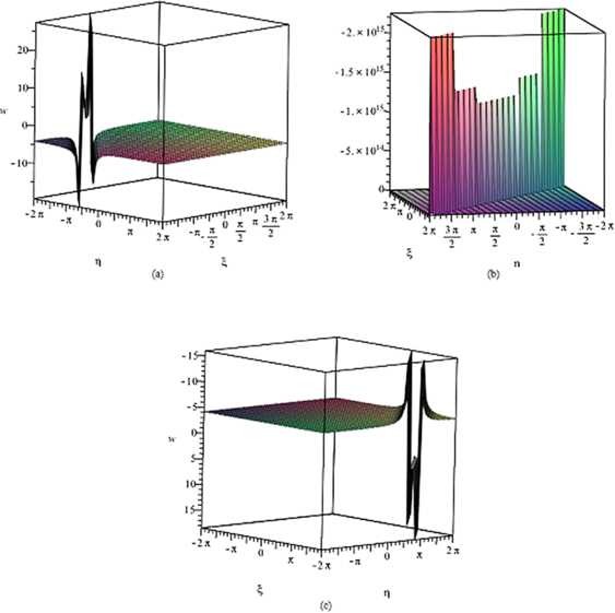
The solution of the gZK equation corresponding to \(\pmb{W_{s,2}(z)}\) . (a) \(z_{0}=-8\), (b) \(z_{0}=0\), (c) \(z_{0}=8\).
-
(2)
By using the complex method, we achieve to obtain simply periodic solutions \(W_{s}(z)\) of the YSTF equation. The solutions \(W_{s}(z)\) are in terms of the hyperbolic function solution. The solutions \(W_{s}(z)\) in Figure 2 of the YSTF equation are represented the singular soliton solution for the parameters \(k=1\), \(l=1\), \(r=1\), \(\alpha=1\) and \(y=0\) within the interval \(-2\pi\leq\xi, \eta\leq2\pi\).
Figure 2 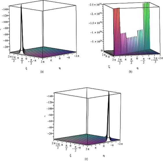
The solution of the YSTF equation corresponding to \(\pmb{W_{s}(z)}\) . (a) \(z_{0}=-8\), (b) \(z_{0}=0\), (c) \(z_{0}=8\).


6 Conclusions
In this article, we utilize Lie group analysis to obtain symmetries and symmetry reduction for two higher-dimensional NLEEs. In this way, we can reduce the dimension of the NLEEs, which is relevant in the fields of mathematical physics and engineering. Five types of explicit function solutions are constructed by the \(\exp(-\phi(z))\)-expansion method and complex method. It demonstrates these methods are very efficient and powerful to seek the exact solutions of NLEEs. We can apply the idea of this study to other NLEEs.
References
Yu, S, Toda, K, Sasa, N, Fukuyama, T: N soliton solutions to the Bogoyavlenskii-Schiff equation and a quest for the soliton solution in \((3+1)\) dimensions. J. Phys. A, Math. Gen. 31(14), 3337-3347 (1998)
Mei, JQ, Zhang, HQ: New soliton-like and periodic-like solutions for the KdV equation. Appl. Math. Comput. 169, 589-599 (2005)
Cui, AG, Li, HY, Zhang, CY: A splitting method for shifted skew-Hermitian linear system. J. Inequal. Appl. 2016, 160 (2016)
Khalique, CM, Adem, KR: Exact solutions of the \((2+1)\) dimensional Zakharov-Kuznetsov modified equal width equation using Lie group analysis. Math. Comput. Model. 54(1-2), 184-189 (2011)
Wazwaz, AM: New solitons and kink solutions for the Gardner equation. Commun. Nonlinear Sci. Numer. Simul. 12, 1395-1404 (2007)
Tascan, F, Bekir, A, Koparan, M: Travelling wave solutions of nonlinear evolution equations by using the first integral method. Commun. Nonlinear Sci. Numer. Simul. 14(5), 1810-1815 (2009)
Roshid, HO, Alam, MN, Akbar, MA: Traveling wave solutions for fifth order \((1+ 1)\)-dimensional Kaup-Keperschmidt equation with the help of \(\operatorname{Exp}(-\phi\eta)\)-expansion method. Walailak J. Sci. Technol. 12(11), 1063-1073 (2015)
Roshid, HO, Alam, MN, Akbar, MA, Islam, R: Traveling wave solutions of the simplified MCH equation via \(\operatorname{Exp}(-\varPhi (\xi))\)-expansion method. Br. J. Math. Comput. Sci. 5(5), 595-605 (2015)
Roshid, HO, Kabir, MR, Bhowmik, RC, Datta, BK: Investigation of solitary wave solutions for Vakhnenko-Parkes equation via exp-function and \(\operatorname{Exp}(-\phi(\xi))\)-expansion method. SpringerPlus 3, 692 (2014)
Roshid, HO, Roshid, MM, Rahman, N, Pervin, MR: New solitary wave in shallow water, plasma and ion acoustic plasma via the GZK-BBM equation and the RLW equation. Propuls. Power Res. 6(1), 49-57 (2017)
Roshid, HO: Novel solitary wave solution in shallow water and ion acoustic plasma waves in-terms of two nonlinear models via MSE method. J. Ocean Eng. Sci. 2(3), 196-202 (2017)
Roshid, HO, Rashidi, MM: Multi-soliton fusion phenomenon of Burgers equation and fission, fusion phenomenon of Sharma-Tasso-Olver equation. J. Ocean Eng. Sci. 2(2), 120-126 (2017)
Roshid, HO: Lump solutions to a \((3+1)\)-dimensional potential-Yu-Toda-Sasa-Fukuyama (YTSF) like equation. Int. J. Appl. Comput. Math. 3, 1455-1461 (2017)
Zakharov, VE, Kuznetsov, EA: On three-dimensional solitons. Sov. Phys. JETP 39, 285-288 (1974)
Toh, S, Iwasaki, H, Kawahara, T: Two-dimensionally localized pulses of a nonlinear equation with dissipation and dispersion. Phys. Rev. A 40, 5472-5475 (1989)
Petviashvihi, VI: Red spot of Jupiter and the drift soliton in plasma. JETP Lett. 32, 619-622 (1980)
Nozaki, K: Vortex solutions of drift waves and anomalous diffusion. Phys. Rev. Lett. 46, 184-187 (1981)
Li, B, Chen, Y, Zhang, H: Auto-Bäcklund transformation and exact solutions for compound KdV-type and compound KdV-Burgers-type equations with nonlinear terms of any order. Phys. Lett. A 305(6), 377-382 (2002)
Taghizadeh, N, Neirameh, A: New complex solutions for some special nonlinear partial differential systems. Comput. Math. Appl. 62(4), 2037-2044 (2011)
Jawad, AJM, Petkovic, MD, Biswas, A: Modified simple equation method for nonlinear evolution equations. Appl. Math. Comput. 217(2), 869-877 (2010)
Tian, C: Lie Group and Its Applications in Partial Differential Equations. Higher Education Press, Beijing (2001)
Liu, H, Li, J, Zhang, Q: Lie symmetry analysis and exact explicit solutions for general Burgers’ equation. J. Comput. Appl. Math. 228(1), 1-9 (2009)
Islam, SMR, Khan, K, Akbar, MA: Exact solutions of unsteady Korteweg-de Vries and time regularized long wave equations. SpringerPlus 4, 124 (2015)
Khan, K, Akbar, MA: The \(\exp(-\phi(\xi))\)-expansion method for finding travelling wave solutions of Vakhnenko-Parkes equation. Int. J. Dyn. Syst. Differ. Equ. 5(1), 72-83 (2014)
Yuan, WJ, Xiao, B, Wu, YH, Qi, JM: The general traveling wave solutions of the Fisher type equations and some related problems. J. Inequal. Appl. 2014, 500 (2014)
Yuan, WJ, Huang, ZF, Fu, MZ, Lai, JC: The general solutions of an auxiliary ordinary differential equation using complex method and its applications. Adv. Differ. Equ. 2014, 147 (2014)
Yuan, WJ, Meng, FN, Huang, Y, Wu, YH: All traveling wave exact solutions of the variant Boussinesq equations. Appl. Math. Comput. 268, 865-872 (2015)
Lang, S: Elliptic Functions, 2nd edn. Springer, New York (1987)
Eremenko, A, Liao, LW, Ng, TW: Meromorphic solutions of higher order Briot-Bouquet differential equations. Math. Proc. Camb. Philos. Soc. 146, 197-206 (2009)
Yuan, WJ, Shang, YD, Huang, Y, Wang, H: The representation of meromorphic solutions to certain ordinary differential equations and its applications. Sci. Sin., Math. 43(6), 563-575 (2013)
Kudryashov, NA: Meromorphic solutions of nonlinear ordinary differential equations. Commun. Nonlinear Sci. Numer. Simul. 15(10), 2778-2790 (2010)
Acknowledgements
This work was supported by the NSF of China (11271090, 11701111); the NSF of Guangdong Province (2016A030310257); the Foundation for Young Talents in Educational Commission of Guangdong Province (2015KQNCX116). Thanks to the Joint PHD Program of Guangzhou University and Curtin University. Thanks to the editors and referees with their very useful suggestions and helpful comments.
Author information
Authors and Affiliations
Contributions
All authors typed, read and approved the final manuscript.
Corresponding author
Ethics declarations
Competing interests
The authors declare that they have no competing interests.
Additional information
Publisher’s Note
Springer Nature remains neutral with regard to jurisdictional claims in published maps and institutional affiliations.
Rights and permissions
Open Access This article is distributed under the terms of the Creative Commons Attribution 4.0 International License (http://creativecommons.org/licenses/by/4.0/), which permits unrestricted use, distribution, and reproduction in any medium, provided you give appropriate credit to the original author(s) and the source, provide a link to the Creative Commons license, and indicate if changes were made.
About this article

Cite this article
Gu, Y., Qi, J. Symmetry reduction and exact solutions of two higher-dimensional nonlinear evolution equations. J Inequal Appl 2017, 314 (2017). https://doi.org/10.1186/s13660-017-1587-5
Received:
Accepted:
Published:
DOI: https://doi.org/10.1186/s13660-017-1587-5