Theoretical and computational results of a wave equation with variable exponent and time-dependent nonlinear damping

Abstract

We study the following wave equation $u_{tt}-\Delta u+\alpha (t)\left| u_{t}\right| ^{m(\cdot )-2}u_{t}=0$ with a nonlinear damping having a variable exponent m(x) and a time-dependent coefficient $\alpha (t)$. We use the multiplier method to establish energy decay results depending on both m and $\alpha$. We also give four numerical tests to illustrate our theoretical results using the conservative Lax–Wendroff method scheme.

1 Introduction

In this paper we are concerned with the following problem:

$$\begin{aligned} \left\{ \begin{array}{l} u_{tt}-\Delta u+\alpha (t)\left| u_{t}\right| ^{m(\cdot )-2}u_{t}=0,\qquad \text {in }\Omega \times (0,T), \\ u=0,\qquad \text {on }\partial \Omega \times (0,T), \\ u(x,0)=u_{0}(x), u_{t}(x,0)=u_{1}(x), x\in \Omega . \end{array} \right. \end{aligned}$$

(1.1)

This is a weakly damped wave equation associated with homogeneous Dirichlet boundary conditions and initial data in suitable function spaces. Here, $\Omega$ is a bounded domain of ${\mathbb {R}}^{n}$ $(n\ge 1)$ with a smooth boundary $\partial \Omega$,

$$\begin{aligned} \alpha :[0,\infty )\rightarrow (0,\infty )\text { is a nonincreasing }C^{1} \text {-function} \end{aligned}$$

(1.2)

and $m\in C^{1}({\overline{\Omega }})$ is satisfying

$$\begin{aligned} 1<m_{1}\le m(x)\le m_{2}<2^{*}, \end{aligned}$$

(1.3)

with

$$\begin{aligned} m_{1}=\underset{x\in \Omega }{\inf }m(x),\qquad m_{2}=\underset{x\in \Omega }{\sup }m(x),\qquad 2^{*}=\left\{ \begin{array}{c} \frac{2n}{n-2},\qquad \text {if }n>2 \\ \infty ,\qquad \text {if }n=1,2 \end{array} \right. , \end{aligned}$$

and also satisfying the log-Hölder continuity condition:

$$\begin{aligned} \left| m(x)-m(y)\right| \le -\frac{A}{\log \left| x-y\right| },\quad \text {for all } x,y\in \Omega \text { with }\left| x-y\right|<\delta ,0<\delta <1,A>0. \end{aligned}$$

(1.4)

In the case when m is a constant satisfying $1<m<2^{*}$, there have been many results concerning the existence and energy decay rates of the solutions, we refer the readers to [6, 12, 14, 26, 28] and the references therein. Similar results were also obtained for frictional dissipative boundary condition (see [15, 17, 29]). When the damping is competing with a source term of the form $\left| u\right| ^{p-2}u$, ${p \le 2}$ results on finite-time blow-up for $p>m$ and global existence for $p\le m$ have been established in [10, 18, 20, 21].

In recent years, more attention has been paid to the study of mathematical nonlinear models of hyperbolic, parabolic and elliptic equations with variable exponents of nonlinearity. Some models from physical phenomena like flows of electro-rheological fluids or fluids with temperature-dependent viscosity, filtration processes in a porous media, nonlinear viscoelasticity, and image processing, give rise to such problems. More details on the subject can be found in [4, 5]. Regarding hyperbolic problems with nonlinearities of variable-exponent type, only few works have appeared. For instance, Antontsev [2, 3] considered the equation

$$\begin{aligned} u_{tt}-\text {div}(a(x,t)|\nabla u|^{p(x,t)-2}\nabla u)-\alpha \Delta u_{t}=b(x,t)|u|^{\sigma (x,t)-2}u \end{aligned}$$

(1.5)

in a bounded domain $\Omega \subset {\mathbb {R}}^{n}$, with non-positive initial energy. Under appropriate conditions on the functions $a,b,p,\sigma$, the local, global and blow-up solutions have been established. Guo and Gao [11] considered the same problem (1.5) and proved several blow-up results for certain solutions with positive initial energy. The following equation:

$$\begin{aligned} u_{tt}-\text {div}(|\nabla u|^{r(x)-2}\nabla u)+a|u_{t}|^{m(x)-1}u_{t}=b|u|^{p(x)-2}u, \end{aligned}$$

(1.6)

was investigated by Messaoudi and Talahmeh [22, 24]. They established the existence of a unique weak solution using the Faedo–Galerkin method and proved the finite-time blow up of solutions. Moreover, when $r(x)\equiv 2$, Sun et al. [27] gave lower and upper bounds for the blow-up time. Recently, Messaoudi et al. [25] looked at (1.6), with $b=0$ and $2\le m(x)<2^{*}$ , and proved decay estimates for the solution under suitable assumptions on the variable exponents m, r and the initial data. We also refer to Gao and Gao [9] who studied a nonlinear viscoelastic equation with variable exponents and proved the existence of weak solutions.

Our aim in this work is to investigate (1.1), in which the damping considered is modulated by a time-dependent coefficient $\alpha (t)$ satisfying (1.2) and has a variable exponent m(x) satisfying (1.3) and (1.4). We study both cases when $m_{1}\ge 2$ and $m_{1}<2$ and establish explicit energy decay rates depending on both m and $\alpha$. To the best of our knowledge, this latter case has never been discussed for variable-exponent nonlinearity even for $\alpha \equiv 1$. The paper is organized as follows. In Sect. 2, we present some notations and material needed for our work. The statement and the proof of our main results will be given in Sect. 3. In Sect. 4, we give a numerical verification of the theoretical decay results.

2 Preliminaries

In this section, we present some preliminary facts about Lebesgue and Sobolev spaces with variable exponents (see [7, 16]). Let $p:\Omega \rightarrow [1,\infty )$ be a measurable function, where $\Omega$ is a domain of $\mathbb {R}^{n}$. We define the Lebesgue space with a variable exponent $p(\cdot )$ by

$$\begin{aligned} L^{p(\cdot )}(\Omega )=\left\{ u:\Omega \rightarrow {\mathbb {R}}\text { , measurable in }\Omega \text { and }\varrho _{p(\cdot )}(u)=\int _{\Omega }\left| u(x)\right| ^{p(x)}\mathrm{d}x<\infty \right\} . \end{aligned}$$

Equipped with the following Luxembourg-type norm

$$\begin{aligned} \left\| u\right\| _{p(\cdot )}:=\inf \left\{ \lambda >0:\varrho _{p(\cdot )}\left( \frac{u}{\lambda }\right) \le 1\right\} , \end{aligned}$$

$L^{p(\cdot )}(\Omega )$ is a Banach space. If $1<p_{1}\le p(x)\le p_{2}<\infty$ holds, then, for any $u\in L^{p(\cdot )}(\Omega )$,

$$\begin{aligned} \min \{\Vert u\Vert _{p(\cdot )}^{p_{1}},\Vert u\Vert _{p(\cdot )}^{p_{2}}\}\le \varrho _{p(\cdot )}(u)\le \max \{\Vert u\Vert _{p(\cdot )}^{p_{1}},\Vert u\Vert _{p(\cdot )}^{p_{2}}\}. \end{aligned}$$

We, next, define the variable-exponent Sobolev space $W^{1,p(\cdot )}(\Omega )$ as follows:

$$\begin{aligned} W^{1,p(\cdot )}(\Omega )=\{u\in L^{p(\cdot )}(\Omega ):\nabla u\;\text {exists }\;\text {and}\;|\nabla u|\in L^{p(\cdot )}(\Omega )\}. \end{aligned}$$

This space is a Banach space with respect to the norm $\Vert u\Vert _{W^{1,p(\cdot )}(\Omega )}=\Vert u\Vert _{p(\cdot )}+\Vert \nabla u\Vert _{p(\cdot )}.$ Furthermore, we set $W_{0}^{1,p(\cdot )}(\Omega )$ to be the closure of $C_{0}^{\infty }(\Omega )$ in $W^{1,p(\cdot )}(\Omega )$. Here we note that the space $W_{0}^{1,p(\cdot )}(\Omega )$ is usually defined in a different way for the variable exponent case. However, both definitions are equivalent under (1.4).

• Hölder’s inequality: Let $p,q,s\ge 1$ be measurable functions defined on $\Omega$ such that

  $$\begin{aligned} \frac{1}{s(y)}=\frac{1}{p(y)}+\frac{1}{q(y)},\;\;\text {for a.e.}\;\;y\in \Omega . \end{aligned}$$

  If $f\in L^{p(\cdot )}(\Omega )$ and $g\in L^{q(\cdot )}(\Omega )$, then $fg\in L^{s(\cdot )}(\Omega )$ and

  $$\begin{aligned} \Vert fg\Vert _{s(\cdot )}\le \;2\;\Vert f\Vert _{p(\cdot )}\Vert g\Vert _{q(\cdot )}. \end{aligned}$$

• Poincaré’s inequality: Let $\Omega$ be a bounded domain of ${\mathbb {R}}^{n}$ and $p(\cdot )$ satisfies (1.4), then

  $$\begin{aligned} \Vert u\Vert _{p(\cdot )}\le C\Vert \nabla u\Vert _{p(\cdot )},\;\;\;\text { for all}\;\;u\in W_{0}^{1,p(\cdot )}(\Omega ), \end{aligned}$$

  where the positive constant C depends on $p_{1},p_{2}$ and $\Omega$ only. In particular, the space $W_{0}^{1,p(\cdot )}(\Omega )$ has an equivalent norm given by $\Vert u\Vert _{W_{0}^{1,p(\cdot )}(\Omega )}=\Vert \nabla u\Vert _{p(\cdot )}.$

• Embedding property: Let $\Omega$ be a bounded domain in ${\mathbb {R}}^{n}$ with a smooth boundary $\partial \Omega .$ Assume that $p,q\in C({\overline{\Omega }})$ such that

  $$\begin{aligned} 1<p_{1}\le p(x)\le p_{2}<+\infty ,\;\;1<q_{1}\le q(x)\le q_{2}<+\infty ,\;\;\text {for all}\;x\in {\overline{\Omega }}, \end{aligned}$$

  and $q(x)<p^{*}(x)$ in ${\overline{\Omega }}$ with $p^{*}(x)= {\left\{ \begin{array}{ll} \frac{np(x)}{n-p(x)}, &{} \text {if}\;p_{2}<n \\ +\infty , &{} \text {if}\;p_{2}\ge n. \end{array}\right. }$, then there is a continuous and compact embedding $W^{1,p(\cdot )}(\Omega )\hookrightarrow L^{q(\cdot )}(\Omega )$.

To establish our decay results, the following lemmas will be of essential use.

Lemma 2.1

[19] Let $E:{\mathbb {R}} _{+}\rightarrow {\mathbb {R}}_{+}$ be a nonincreasing function and $\sigma :{\mathbb {R}}_{+}\rightarrow {\mathbb {R}}_{+}$ be an increasing $C^{1}$-function, with $\sigma (0)=0$ and $\sigma (t)\rightarrow +\infty$ as $t\rightarrow +\infty .$

Assume that there exist $q\ge 0$ and $w>0$ such that

$$\begin{aligned} \int \limits _{S}^{\infty }\sigma ^{\prime }(t)E(t)^{q+1}\mathrm{d}t\le \frac{1}{w}E(S),\qquad 0\le S<+\infty . \end{aligned}$$

Then there exists a positive constant k depending continuously on E(0) such that, $\forall t\ge 0$,

$$\begin{aligned} E(t)\le & {} ke^{-w\sigma (t)},\quad \mathrm {if }\quad q=0, \\ E(t)\le & {} \frac{k}{\left[ 1+\sigma (t)\right] ^{\frac{1}{q}}},\quad \mathrm {if} \quad q>0. \end{aligned}$$

Lemma 2.2

(Gagliardo–Nirenberg interpolation inequality) The inequality

$$\begin{aligned} \left\| v\right\| _{p}\le c\left\| v\right\| _{1,2}^{\theta }\left\| v\right\| _{2}^{1-\theta },\qquad \forall v\in W^{1,2}(\Omega ), \end{aligned}$$

holds for some $c>0$ and any $p>2$ where

$$\begin{aligned} \theta =n\left( \frac{1}{2}-\frac{1}{p}\right) \quad \text {and}\quad { \Vert v\Vert _{1,2}=\Vert v\Vert _{2}+\Vert \nabla v\Vert _2.} \end{aligned}$$

At the end of this section, we state the following existence and regularity result, whose proof can be established similarly to [23, 24].

Proposition 2.3

Let $(u_{0},u_{1})\in H_{0}^{1}(\Omega )\times L^{2}(\Omega )$ be given. Assume that (1.2)–(1.4) are satisfied, then problem (1.1) has a unique global (weak) solution

$$\begin{aligned} u\in L^{\infty }((0,\infty );H_{0}^{1}(\Omega )),u_{t}\in L^{\infty }((0,\infty );L^{2}(\Omega ))\cap L^{m(\cdot )}((0,\infty )\times \Omega ). \end{aligned}$$

Moreover, if $(u_{0},u_{1})\in \left( H^{2}(\Omega )\cap H_{0}^{1}(\Omega )\right) \times H_{0}^{1}(\Omega )$, then the solution satisfies

$$\begin{aligned} u\in L^{\infty }((0,\infty );H^{2}(\Omega )\cap H_{0}^{1}(\Omega ))\cap W^{1,\infty }((0,\infty );H_{0}^{1}(\Omega ))\cap W^{2,\infty }((0,\infty );L^{2}(\Omega )). \end{aligned}$$

3 The main results

We define the energy functional by

$$\begin{aligned} E(t):=\frac{1}{2}\int _{\Omega }\left( u_{t}^{2}+\left| \nabla u\right| ^{2}\right) \mathrm{d}x. \end{aligned}$$

(3.1)

Simple calculations show

$$\begin{aligned} E^{\prime }(t)=-\alpha (t)\int _{\Omega }\left| u_{t}\right| ^{m(x)}\mathrm{d}x\le 0, \end{aligned}$$

(3.1*)

which means that E(t) is a nonincreasing function. Let us mention that we will use c, throughout this paper, to denote a generic positive constant. Now, we state and prove our first result.

Theorem 3.1

Assume that (1.2)–(1.4), $m_{1}\ge 2$ , and $\int _{0}^{\infty }\alpha (t)\mathrm{d}t=\infty$. Then there exist positive constants k and w such that the solution of (1.1) satisfies, $\forall t\ge 0$,

$$\begin{aligned} E(t)\le \left\{ \begin{array}{c} ke^{-w\int _{0}^{t}\alpha (s)ds},\qquad \text {if } \qquad m_{2}=2 \\ \frac{k}{\left( 1+\int _{0}^{t}\alpha (s)ds\right) ^{\frac{2}{m_{2}-2}}} ,\qquad \text {if }\qquad m_{2}>2. \end{array} \right. \end{aligned}$$

(3.2)

Proof

We multiply (1.1) $_{1}$ by $\alpha E^{q}u$, for $q\ge 0$ to be specified later, and integrate over $\Omega \times (S,T)$ to get

$$\begin{aligned} 0= & {} \int _{S}^{T}\alpha (t)E^{q}(t)\int _{\Omega }\left( uu_{tt}-u\Delta u+\alpha (t)\left| u_{t}\right| ^{m(x)-2}u_{t}u\right) \mathrm{d}x\mathrm{d}t \\= & {} \int _{S}^{T}\alpha (t)E^{q}(t)\int _{\Omega }\left( \left( uu_{t}\right) _{t}-u_{t}^{2}+\left| \nabla u\right| ^{2}+\alpha (t)\left| u_{t}\right| ^{m(x)-2}u_{t}u\right) \mathrm{d}x\mathrm{d}t \\= & {} \int _{S}^{T}\alpha (t)E^{q}(t)\frac{d}{\mathrm{d}t}\left( \int _{\Omega }uu_{t}\mathrm{d}x\right) \mathrm{d}t+\int _{S}^{T}\alpha (t)E^{q}(t)\int _{\Omega }\left( u_{t}^{2}+\left| \nabla u\right| ^{2}\right) \mathrm{d}x\mathrm{d}t \\&-2\int _{S}^{T}\alpha (t)E^{q}(t)\int _{\Omega }u_{t}^{2}\mathrm{d}x\mathrm{d}t+\int _{S}^{T}\alpha ^{2}(t)E^{q}(t)\int _{\Omega }\left| u_{t}\right| ^{m(x)-2}u_{t}u\mathrm{d}x\mathrm{d}t. \end{aligned}$$

Integrating by parts in the first term, using the definition of E(t), leads to

$$\begin{aligned} 2\int _{S}^{T}\alpha E^{q+1}\mathrm{d}t=&-\left[ \alpha E^{q}\int _{\Omega }uu_{t}\mathrm{d}x \right] _{S}^{T}+\int _{S}^{T}\left( \alpha ^{\prime }E^{q}+q\alpha E^{q-1}E^{\prime }\right) \int _{\Omega }uu_{t}\mathrm{d}x\mathrm{d}t\nonumber \\&+2\int _{S}^{T}\alpha E^{q}\int _{\Omega }u_{t}^{2}\mathrm{d}x\mathrm{d}t-\int _{S}^{T}\alpha ^{2}E^{q}\int _{\Omega }\left| u_{t}\right| ^{m(x)-2}u_{t}u\mathrm{d}x\mathrm{d}t\nonumber \\ = \,&I_1+I_2+I_3+I_4. \end{aligned}$$

(3.3)

We estimate the terms in the right-hand side as follows:

• $I_{1}:=$ $-\left[ \alpha E^{q}\int _{\Omega }uu_{t}\mathrm{d}x \right] _{S}^{T}.$

  Using Young’s and Poincaré’s inequalities, we have

  $$\begin{aligned} \int _{\Omega }uu_{t}\mathrm{d}x\le \frac{1}{2}\int _{\Omega }\left( u^{2}+u_{t}^{2}\right) \mathrm{d}x\le c\int _{\Omega }\left( \left| \nabla u\right| ^{2}+u_{t}^{2}\right) \mathrm{d}x\le cE(t), \end{aligned}$$

  then, by the properties of E and $\alpha ,$ we conclude that

  $$\begin{aligned} I_{1}\le c[\alpha (T)E^{q+1}(T)+\alpha (S)E^{q+1}(S)]\le c\alpha (S)E^{q+1}(S)\le cE(S). \end{aligned}$$

• $I_{2}:=\int _{S}^{T}\left( \alpha ^{\prime }E^{q}+q\alpha E^{q-1}E^{\prime }\right) \int _{\Omega }uu_{t}\mathrm{d}x\mathrm{d}t$.

  As in above,  we conclude that

  $$\begin{aligned} I_{2}\le & {} c\left| \int _{S}^{T}\alpha ^{\prime }E^{q+1}\mathrm{d}t\right| +c\left| \int _{S}^{T}\alpha E^{q}E^{\prime }\mathrm{d}t\right| \\\le & {} cE(S)^{q+1}\left| \int _{S}^{T}\alpha ^{\prime }\mathrm{d}t\right| +c\alpha (S)\left| \int _{S}^{T}E^{q}E^{\prime }\mathrm{d}t\right| \\\le & {} c\alpha (S)E^{q+1}(S)\le cE(S). \end{aligned}$$

• $I_{3}:=2\int _{S}^{T}\alpha E^{q}\int _{\Omega }u_{t}^{2}\mathrm{d}x\mathrm{d}t$.

  If $m_{2}=2$, then

  $$\begin{aligned} I_{3}=2\int _{S}^{T}E^{q}\left( -E^{\prime }\right) \mathrm{d}t=\frac{2}{q+1} [E^{q+1}(S)-E^{q+1}(T)]\le cE(S). \end{aligned}$$

  If $m_{2}>2$, we consider the partition of $\Omega$ (see [19]),

  $$\begin{aligned} \Omega _{1}=\{x\in \Omega :\left| u_{t}\right| \ge 1\}\quad \text { and}\quad \Omega _{2}=\{x\in \Omega :\left| u_{t}\right| <1\} \end{aligned}$$

  and make use of Hölder’s and Young’s inequalities and (3.1) as follows:

  $$\begin{aligned} \alpha \int _{\Omega _{1}}u_{t}^{2}\mathrm{d}x\le & {} \alpha \int _{\Omega }\left| u_{t}\right| ^{m(x)}\mathrm{d}x= -E^{\prime }(t) , \\ \alpha \int _{\Omega _{2}}u_{t}^{2}\mathrm{d}x\le & {} c\alpha \left( \int _{\Omega _{2}}\left| u_{t}\right| ^{m_{2}}\mathrm{d}x\right) ^{\frac{2}{m_{2}}} \\\le & {} c\alpha \left( \int _{\Omega _{2}}\left| u_{t}\right| ^{m(x)}\mathrm{d}x\right) ^{\frac{2}{m_{2}}}\le c\alpha ^{1-\frac{2}{m_{2}}}\left( \alpha \int _{\Omega }\left| u_{t}\right| ^{m(x)}\mathrm{d}x\right) ^{\frac{2}{ m_{2}}}=c\alpha ^{1-\frac{2}{m_{2}}}\left( -E^{\prime }(t)\right) ^{\frac{2}{ m_{2}}}, \end{aligned}$$

  which gives, for all $\delta >0$,

  $$\begin{aligned} I_{3}\le & {} c\int _{S}^{T}E^{q}\left( -E^{\prime }\right) \mathrm{d}t+c\int _{S}^{T}E^{q}\alpha ^{1-\frac{2}{m_{2}}}\left( -E^{\prime }\right) ^{ \frac{2}{m_{2}}}\mathrm{d}t\\\le & {} c[E^{q+1}(S)-E^{q+1}(T)]+c\delta \int _{S}^{T}\alpha ^{\left( 1-\frac{2}{ m_{2}}\right) \left( \frac{q+1}{q}\right) }E^{q+1}\mathrm{d}t+C_{\delta }\int _{S}^{T}\left( -E^{\prime }\right) ^{\frac{2(q+1)}{m_{2}}}\mathrm{d}t. \end{aligned}$$

  We choose $\delta =\frac{1}{2c}$, $q=\frac{m_{2}}{2}-1$, so $\frac{2(q+1)}{m_{2}}=1$ and $\left( 1-\frac{2}{m_{2}}\right) \left( \frac{q+1}{q}\right) =1$, and we arrive at

  $$\begin{aligned} I_{3}\le \frac{1}{2}\int _{S}^{T}\alpha E^{q+1}\mathrm{d}t+cE(S). \end{aligned}$$

• $I_{4}:=-\int _{S}^{T}\alpha ^{2}E^{q}\int _{\Omega }\left| u_{t}\right| ^{m(x)-2}u_{t}u\mathrm{d}x\mathrm{d}t$.

  Here, we use Young’s inequality with $p(x)=\frac{m(x)}{m(x)-1}$ and $p^{\prime }(x)=m(x)$. So, for all $x\in \Omega$, we have

  $$\begin{aligned} \left| u_{t}\right| ^{m(x)-2}u_{t}u\le \varepsilon \left| u\right| ^{m(x)}+C_{\varepsilon }(x)\left| u_{t}\right| ^{m(x)}, \end{aligned}$$

  where

  $$\begin{aligned} C_{\varepsilon }(x)=\frac{\left[ m(x)-1\right] ^{m(x)-1}}{ [m(x)]^{m(x)}\varepsilon ^{m(x)-1}}. \end{aligned}$$

  Therefore, for all $\varepsilon$, we get

  $$\begin{aligned} I_{4}\le & {} \varepsilon \int _{S}^{T}\alpha ^{2}E^{q}\int _{\Omega }\left| u\right| ^{m(x)}\mathrm{d}x\mathrm{d}t+\int _{S}^{T}\alpha ^{2}E^{q}\int _{\Omega }C_{\varepsilon }(x)\left| u_{t}\right| ^{m(x)}\mathrm{d}x\mathrm{d}t \\\le & {} c\varepsilon \int _{S}^{T}\alpha E^{q}\int _{\Omega }\left( \left| u\right| ^{m_{1}}+\left| u\right| ^{m_{2}}\right) \mathrm{d}x\mathrm{d}t+c\int _{S}^{T}\alpha E^{q}\int _{\Omega }C_{\varepsilon }(x)\left| u_{t}\right| ^{m(x)}\mathrm{d}x\mathrm{d}t \\\le & {} c\varepsilon \int _{S}^{T}\alpha E^{q}\left( \left\| \nabla u\right\| _{2}^{m_{1}}+\left\| \nabla u\right\| _{2}^{m_{2}}\right) \mathrm{d}t+c\int _{S}^{T}\alpha E^{q}\int _{\Omega }C_{\varepsilon }(x)\left| u_{t}\right| ^{m(x)}\mathrm{d}x\mathrm{d}t \\\le & {} c\varepsilon \int _{S}^{T}\alpha E^{q}\left( E^{\frac{m_{1}}{2}}+E^{ \frac{m_{2}}{2}}\right) \mathrm{d}t+c\int _{S}^{T}\alpha E^{q}\int _{\Omega }C_{\varepsilon }(x)\left| u_{t}\right| ^{m(x)}\mathrm{d}x\mathrm{d}t \\\le & {} c\varepsilon \left( E(0)^{\frac{m_{1}}{2}-1}+E(0)^{\frac{m_{2}}{2} -1}\right) \int _{S}^{T}\alpha E^{q+1}\mathrm{d}t+c\int _{S}^{T}\alpha E^{q}\int _{\Omega }C_{\varepsilon }(x)\left| u_{t}\right| ^{m(x)}\mathrm{d}x\mathrm{d}t. \end{aligned}$$

  If we fix $\varepsilon =\frac{1}{2c\left( E(0)^{\frac{m_{1}}{2}-1}+E(0)^{ \frac{m_{2}}{2}-1}\right) }$, then $C_{\varepsilon }(x)$ is bounded since m(x) is bounded. So, we obtain

  $$\begin{aligned} I_{4}\le & {} \frac{1}{2}\int _{S}^{T}\alpha E^{q+1}\mathrm{d}t+c\int _{S}^{T}\alpha E^{q}\int _{\Omega }\left| u_{t}\right| ^{m(x)}\mathrm{d}x\mathrm{d}t \\\le & {} \frac{1}{2}\int _{S}^{T}\alpha E^{q+1}\mathrm{d}t+c\int _{S}^{T}E^{q}\left( -E^{\prime }\right) \mathrm{d}t \\\le & {} \frac{1}{2}\int _{S}^{T}\alpha E^{q+1}\mathrm{d}t+cE(S). \end{aligned}$$

  Inserting all the above estimates into (3.3) and taking $T\rightarrow \infty$, we arrive at

  $$\begin{aligned} \int _{S}^{\infty }\alpha E^{q+1}\mathrm{d}t\le cE(S), \end{aligned}$$

  where $q=\frac{m_{2}}{2}-1$. Hence, using Lemma 2.1 with $\sigma (t)=\int _{0}^{t}\alpha (s)ds$, the estimate (3.2) is established.$\square$

Remark 3.2

Note that the decay result of [25] is only a special case of our result in Theorem 3.1.

Now, to study the case $1<m_{1}<2$, we first need to obtain a uniform bound for the second-order energy defined by

$$\begin{aligned} E_{*}(t):=\frac{1}{2}\int _{\Omega }\left( u_{tt}^{2}+\left| \nabla u_{t}\right| ^{2}\right) \mathrm{d}x. \end{aligned}$$

Differentiating (1.1) $_{1}$ with respect to t, multiplying by $u_{tt}$ and integrating over $\Omega \times (0,T)$, we obtain

$$\begin{aligned} 0= & {} \int _{0}^{T}\int _{\Omega }u_{tt}\left[ u_{ttt}-\Delta u_{t}+\alpha ^{\prime }(t)\left| u_{t}\right| ^{m(x)-2}u_{t}+\alpha (t)(m(x)-1)\left| u_{t}\right| ^{m(x)-2}u_{tt}\right] \mathrm{d}x\mathrm{d}t \\= & {} \int _{0}^{T}\frac{\mathrm{d}}{\mathrm{d}t}\left[ \frac{1}{2}\int _{\Omega }\left( u_{tt}^{2}+\left| \nabla u_{t}\right| ^{2}\right) \mathrm{d}x\right] \mathrm{d}t \\&+\int _{0}^{T}\int _{\Omega }\left[ \alpha ^{\prime }(t)\left| u_{t}\right| ^{m(x)-2}u_{t}u_{tt}+\alpha (t)(m(x)-1)\left| u_{t}\right| ^{m(x)-2}u_{tt}^{2}\right] \mathrm{d}x\mathrm{d}t. \end{aligned}$$

Thus,

$$\begin{aligned} E_{*}(T)-E_{*}(0)= & {} -\int _{0}^{T}\int _{\Omega }\alpha ^{\prime }(t)\left| u_{t}\right| ^{m(x)-2}u_{t}u_{tt}\mathrm{d}x\mathrm{d}t \\&-\int _{0}^{T}\int _{\Omega }\alpha (t)(m(x)-1)\left| u_{t}\right| ^{m(x)-2}u_{tt}^{2}\mathrm{d}x\mathrm{d}t\\= & {} \int _{0}^{T}\int _{\Omega }\left[ \frac{-\alpha ^{\prime }(t)\left| u_{t}\right| ^{m(x)-2}u_{t}}{\sqrt{\alpha (t)(m(x)-1)\left| u_{t}\right| ^{m(x)-2}}}\right] \left[ \sqrt{\alpha (t)(m(x)-1)\left| u_{t}\right| ^{m(x)-2}}u_{tt}\right] \mathrm{d}x\mathrm{d}t \\&-\int _{0}^{T}\int _{\Omega }\alpha (t)(m(x)-1)\left| u_{t}\right| ^{m(x)-2}u_{tt}^{2}\mathrm{d}x\mathrm{d}t \\\le & {} \int _{0}^{T}\int _{\Omega }\left( \frac{1}{4}\left[ \frac{-\alpha ^{\prime }(t)\left| u_{t}\right| ^{m(x)-2}u_{t}}{\sqrt{\alpha (t)(m(x)-1)\left| u_{t}\right| ^{m(x)-2}}}\right] ^{2}+\left[ \sqrt{ \alpha (t)(m(x)-1)\left| u_{t}\right| ^{m(x)-2}}u_{tt}\right] ^{2}\right) \mathrm{d}x\mathrm{d}t \\&-\int _{0}^{T}\int _{\Omega }\alpha (t)(m(x)-1)\left| u_{t}\right| ^{m(x)-2}u_{tt}^{2}\mathrm{d}x\mathrm{d}t \\= & {} \frac{1}{4}\int _{0}^{T}\int _{\Omega }\left( \frac{-\alpha ^{\prime }(t)}{ \alpha (t)}\right) ^{2}\frac{\alpha (t)\left| u_{t}\right| ^{m(x)}}{ (m(x)-1)}\mathrm{d}x\mathrm{d}t. \end{aligned}$$

But, by (1.2) and the condition that $\int _{0}^{\infty }\alpha (t)\mathrm{d}t=\infty ,$ one can see that $\underset{t\rightharpoonup \infty }{\lim }\frac{-\alpha ^{\prime }(t)}{\alpha (t)}\ne \infty$. Indeed, if $\underset{t\rightharpoonup \infty }{\lim }\frac{-\alpha ^{\prime }(t)}{\alpha (t)}= \infty$ then given $M>0$, $\exists A>0$ such that $\frac{-\alpha ^{\prime }(t)}{\alpha (t)}\ge M$, $\forall t>A$. By integration, we obtain $M\int _A^\infty \alpha (t)\mathrm{d}t \le -\int _A^\infty \alpha '(t)\mathrm{d}t\le \alpha (A)$, which contradicts $\int _{A}^{\infty }\alpha (t)\mathrm{d}t= \infty$. Consequently, $\frac{-\alpha ^{\prime }(t)}{ \alpha (t)}$ is bounded; so $\frac{-\alpha ^{\prime }(t)}{\alpha (t)}\le c_{0}$ for some positive constant $c_{0}$. Therefore,

$$\begin{aligned} E_{*}(T)-E_{*}(0)\le \frac{c_{0}^{2}}{4(m_{1}-1)}\int _{0}^{T}\left( -E^{\prime }(t)\right) \mathrm{d}t=\frac{c_{0}^{2}}{4(m_{1}-1)}\left( E(0)-E(T)\right) , \end{aligned}$$

which means that

$$\begin{aligned} E_{*}(T)\le E_{*}(0)+\frac{c_{0}^{2}E(0)}{4(m_{1}-1)}=C_{0},\qquad \forall T>0. \end{aligned}$$

(3.4)

Next, we state and prove our second result.

Theorem 3.3

Assume that (1.2)–(1.4) hold, $m_{1}<2$, and $\int _{0}^{\infty }\alpha (t)\mathrm{d}t=\infty$. Then there exists a positive constant k such that the solution of (1.1) satisfies, $\forall t\ge 0$,

$$\begin{aligned} E(t)\le \frac{k}{\left( 1+\int _{0}^{t}\alpha (s)ds\right) ^{\frac{1}{q}}}, \end{aligned}$$

(3.5)

where

$$\begin{aligned} q=\max \left\{ \frac{(2-m_{1})\left( n-2\right) }{4},\frac{ 2-m_{1}}{2m_{1}-2},\frac{m_{2}-2}{2}\right\} . \end{aligned}$$

Proof

As done in Theorem 3.1, we multiply (1.1) $_{1}$ by $\alpha E^{q}u$, for $q\ge 0$ to be specified later, integrate over $\Omega \times (S,T)$, similarly estimate $I_{1}$ and $I_{2}$ and get

$$\begin{aligned} 2\int _{S}^{T}\alpha E^{q+1}\mathrm{d}t\le cE(S)+2\int _{S}^{T}\alpha E^{q}\int _{\Omega }u_{t}^{2}\mathrm{d}x\mathrm{d}t-\int _{S}^{T}\alpha ^{2}E^{q}\int _{\Omega }\left| u_{t}\right| ^{m(x)-2}u_{t}u\mathrm{d}x\mathrm{d}t. \end{aligned}$$

(3.6)

Then, we re-estimate the last two terms as follows:

• $I_{3}:=2\int _{S}^{T}\alpha E^{q}\int _{\Omega }u_{t}^{2}\mathrm{d}x\mathrm{d}t.$

  We consider the partition of $\Omega \subset {\mathbb {R}} ^{n}$ $(n\ge 1)$

  $$\begin{aligned} \Omega _{1}=\{x\in \Omega :\left| u_{t}\right| \ge 1\}\quad \text { and}\quad \Omega _{2}=\{x\in \Omega :\left| u_{t}\right| <1\} \end{aligned}$$

  and use Hölder’s inequality and (3.1) to obtain for $m_{2}\le 2$,

  $$\begin{aligned} \alpha \int _{\Omega _{2}}u_{t}^{2}\mathrm{d}x\le \alpha \int _{\Omega }\left| u_{t}\right| ^{m(x)}\mathrm{d}x= -E^{\prime }(t), \end{aligned}$$

  (3.7)

  while, if $m_{2}>2$, then

  

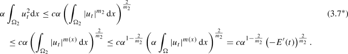
  On $\Omega _{1}$, we have, for a constant $r>1$,

  $$\begin{aligned}&\alpha \int _{\Omega _{1}}u_{t}^{2}\mathrm{d}x=\alpha \int _{\Omega _{1}}|u_{t}|^{\frac{1}{r}}|u_{t}|^{2-\frac{1}{r}}\mathrm{d}x\le \alpha \left( \int _{\Omega _{1}}\left| u_{t}\right| ^{m_{1}}\mathrm{d}x\right) ^{\frac{1}{m_{1}r}}\left( \int _{\Omega _{1}}\left| u_{t}\right| ^{\frac{m_{1}(2r-1)}{m_{1}r-1}}\mathrm{d}x\right) ^{\frac{m_{1}r-1}{m_{1}r}} \nonumber \\&\quad \le \alpha ^{1-\frac{1}{m_{1}r}}\left( \alpha \int _{\Omega }\left| u_{t}\right| ^{m(x)}\mathrm{d}x\right) ^{\frac{1}{m_{1}r}}\left\| u_{t}\right\| _{\frac{m_{1}(2r-1)}{m_{1}r-1}}^{\frac{2r-1}{r}}=\alpha ^{1- \frac{1}{m_{1}r}}\left( -E^{\prime }\right) ^{\frac{1}{m_{1}r}}\left\| u_{t}\right\| _{\frac{m_{1}(2r-1)}{m_{1}r-1}}^{\frac{2r-1}{r}}. \end{aligned}$$

  (3.8)

  But, by the aid of Lemma 2.2, we have

  $$\begin{aligned} \left\| u_{t}\right\| _{\frac{m_{1}(2r-1)}{m_{1}r-1}}\le c\left\| u_{t}\right\| _{1,2}^{\theta }\left\| u_{t}\right\| _{2}^{1-\theta }, \end{aligned}$$

  where $\theta =\frac{(2-m_{1})n}{2m_{1}(2r-1)}$, and since we need $0<\theta \le 1$ then r should be chosen so that $r\ge \frac{(2-m_{1})n+2m_{1}}{ 4m_{1}}$. Then we use (3.4) to find that

  $$\begin{aligned} \left\| u_{t}\right\| _{\frac{m_{1}(2r-1)}{m_{1}r-1}}^{\frac{2r-1}{r} }\le \left[ cC_{0}^{\frac{\theta }{2}}\left( \left\| u_{t}\right\| _{2}^{2}\right) ^{\frac{1-\theta }{2}}\right] ^{\frac{2r-1}{r}}\le c\left( E(t)\right) ^{\frac{2m_{1}(2r-1)-(2-m_{1})n}{4m_{1}r}}. \end{aligned}$$

  (3.9)

  Combination of (3.7), (3.8) and (3.9) yields, for $m_{2}\le 2$,

  $$\begin{aligned} I_{3}&\le c\int _{S}^{T}E^{q}\left( -E^{\prime }\right) \mathrm{d}t+c\int _{S}^{T}E^{q}\alpha ^{1-\frac{1}{m_{1}r}}\left( -E^{\prime }\right) ^{\frac{1}{m_{1}r}}\left( E\right) ^{\frac{2m_{1}(2r-1)-(2-m_{1})n}{4m_{1}r} }\mathrm{d}t\\&\le c[E^{q+1}(S)-E^{q+1}(T)]+c\delta \int _{S}^{T}\alpha E^{\left( q+\frac{ 2m_{1}(2r-1)-(2-m_{1})n}{4m_{1}r}\right) \left( \frac{m_{1}r}{m_{1}r-1} \right) }\mathrm{d}t+C_{\delta }\int _{S}^{T}\left( -E^{\prime }\right) \mathrm{d}t, \; \forall \delta >0. \end{aligned}$$

  If we choose any q satisfying

  $$\begin{aligned} q\ge \left\{ \begin{array}{c} \frac{(2-m_{1})(n-2)}{4},\qquad \text {if }n>2 \\ 0,\qquad \qquad \qquad \qquad \quad \ \, \text {if }n=1\text { or }2 \end{array} \right. , \end{aligned}$$

  (3.10)

  then $\left( q+\frac{2m_{1}(2r-1)-(2-m_{1})n}{4m_{1}r}\right) \left( \frac{ m_{1}r}{m_{1}r-1}\right) \ge q+1$, so, with $\delta$ small enough, we arrive at

  $$\begin{aligned} I_{3}\le \frac{1}{2}\int _{S}^{T}\alpha E^{q+1}\mathrm{d}t+cE(S). \end{aligned}$$

  But, in the case $m_{2}>2$, we use (3.7*), (3.8) and (3.9) to get, for all $\lambda >0$,

  $$\begin{aligned} I_{3}\le & {} c\int _{S}^{T}E^{q}\alpha ^{1-\frac{2}{m_{2}}}\left( -E^{\prime }\right) ^{\frac{2}{m_{2}}}\mathrm{d}t+c\int _{S}^{T}E^{q}\alpha ^{1-\frac{1}{m_{1}r} }\left( -E^{\prime }\right) ^{\frac{1}{m_{1}r}}\left( E\right) ^{\frac{ 2m_{1}(2r-1)-(2-m_{1})n}{4m_{1}r}}\mathrm{d}t\\\le & {} c\lambda \int _{S}^{T}\alpha E^{q\left( \frac{m_{2}}{m_{2}-2}\right) }\mathrm{d}t+C_{\lambda }\int _{S}^{T}\left( -E^{\prime }\right) \mathrm{d}t+c\lambda \int _{S}^{T}\alpha E^{\left( q+\frac{2m_{1}(2r-1)-(2-m_{1})n}{4m_{1}r} \right) \left( \frac{m_{1}r}{m_{1}r-1}\right) }\mathrm{d}t+B_{\lambda }\int _{S}^{T}\left( -E^{\prime }\right) \mathrm{d}t. \end{aligned}$$

  If we choose $q\ge \frac{m_{2}-2}{2}$, provided (3.10) is satisfied, then the following inequalities

  $$\begin{aligned} q\left( \frac{m_{2}}{m_{2}-2}\right) \ge q+1\; \mathrm {and} \; \left( q+\frac{ 2m_{1}(2r-1)-(2-m_{1})n}{4m_{1}r}\right) \left( \frac{m_{1}r}{m_{1}r-1} \right) \ge q+1 \end{aligned}$$

  hold. Hence, with $\lambda$ small enough, we similarly arrive at

  $$\begin{aligned} I_{3}\le \frac{1}{2}\int _{S}^{T}\alpha E^{q+1}\mathrm{d}t+cE(S). \end{aligned}$$

  (3.11)

  Thus, (3.11) is obtained for both cases under the condition that

  $$\begin{aligned} q\ge \max \{\frac{(2-m_{1})\left( n-2\right) }{4},\frac{m_{2}-2}{2}\}. \end{aligned}$$

  (3.12)

• $I_{4}:=-\int _{S}^{T}\alpha ^{2}E^{q}\int _{\Omega }\left| u_{t}\right| ^{m(x)-2}u_{t}u\mathrm{d}x\mathrm{d}t$.

  First, we consider the following partition of $\Omega$

  $$\begin{aligned} \Omega _{*}=\{x\in \Omega :m(x)<2\}\quad \text {and}\quad \Omega _{**}=\{x\in \Omega :m(x)\ge 2\} \end{aligned}$$

  and see that

  $$\begin{aligned} I_{4}\le \int _{S}^{T}\alpha ^{2}E^{q}\int _{\Omega _{*}}\left| u_{t}\right| ^{m(x)-1}\left| u\right| \mathrm{d}x\mathrm{d}t+\int _{S}^{T}\alpha ^{2}E^{q}\int _{\Omega _{**}}\left| u_{t}\right| ^{m(x)-1}\left| u\right| \mathrm{d}x\mathrm{d}t. \end{aligned}$$

  (3.13)

  If $meas\left( \Omega _{**}\right) \ne 0$ so $m_{2}\ge 2$, then, as done in the proof of Theorem 3.1, we use Young’s inequality with $p(x)= \frac{m(x)}{m(x)-1}$ and $p^{\prime }(x)=m(x)$ for $x\in \Omega _{**}$, to obtain

  $$\begin{aligned}&\int _{S}^{T}\alpha ^{2}E^{q}\int _{\Omega _{**}}\left| u_{t}\right| ^{m(x)-1}\left| u\right| \mathrm{d}x\mathrm{d}t\\&\quad \le \int _{S}^{T}\alpha ^{2}E^{q}\int _{\Omega _{**}}\left[ \varepsilon \left| u\right| ^{m(x)}+C_{\varepsilon }(x)\left| u_{t}\right| ^{m(x)}\right] \mathrm{d}x\mathrm{d}t \\&\quad \le c\varepsilon \int _{S}^{T}\alpha E^{q}\int _{\Omega _{**}}\left( \left| u\right| ^{2}+\left| u\right| ^{m_{2}}\right) \mathrm{d}x\mathrm{d}t+c\int _{S}^{T}\alpha E^{q}\int _{\Omega _{**}}C_{\varepsilon }(x)\left| u_{t}\right| ^{m(x)}\mathrm{d}x\mathrm{d}t \\&\quad \le c\varepsilon \int _{S}^{T}\alpha E^{q}\left( \left\| \nabla u\right\| _{2}^{2}+\left\| \nabla u\right\| _{2}^{m_{2}}\right) \mathrm{d}t+c\int _{S}^{T}\alpha E^{q}\int _{\Omega _{**}}C_{\varepsilon }(x)\left| u_{t}\right| ^{m(x)}\mathrm{d}x\mathrm{d}t \\&\quad \le c\varepsilon \int _{S}^{T}\alpha E^{q}\left( E+E^{\frac{m_{2}}{2} }\right) \mathrm{d}t+c\int _{S}^{T}\alpha E^{q}\int _{\Omega _{**}}C_{\varepsilon }(x)\left| u_{t}\right| ^{m(x)}\mathrm{d}x\mathrm{d}t \\&\quad \le c\varepsilon \left( 1+E(0)^{\frac{m_{2}}{2}-1}\right) \int _{S}^{T}\alpha E^{q+1}\mathrm{d}t+c\int _{S}^{T}\alpha E^{q}\int _{\Omega _{**}}C_{\varepsilon }(x)\left| u_{t}\right| ^{m(x)}\mathrm{d}x\mathrm{d}t. \end{aligned}$$

  If we fix $\varepsilon =\frac{1}{4c\left( 1+E(0)^{\frac{m_{2}}{2}-1}\right) }$ , then $C_{\varepsilon }(x)=\frac{\left[ m(x)-1\right] ^{m(x)-1}}{ [m(x)]^{m(x)}\varepsilon ^{m(x)-1}}$ is bounded since m(x) is bounded on $\Omega _{**}$, and we get

  $$\begin{aligned}&\int _{S}^{T}\alpha ^{2}E^{q}\int _{\Omega _{**}}\left| u_{t}\right| ^{m(x)-1}\left| u\right| \mathrm{d}x\mathrm{d}t\le \frac{1}{4} \int _{S}^{T}\alpha E^{q+1}\mathrm{d}t+c\int _{S}^{T}\alpha E^{q}\int _{\Omega }\left| u_{t}\right| ^{m(x)}\mathrm{d}x\mathrm{d}t\nonumber \\&\quad \le \frac{1}{4}\int _{S}^{T}\alpha E^{q+1}\mathrm{d}t+c\int _{S}^{T}E^{q}\left( -E^{\prime }\right) \mathrm{d}t\le \frac{1}{4}\int _{S}^{T}\alpha E^{q+1}\mathrm{d}t+cE(S). \end{aligned}$$

  (3.14)

  On the other hand, we have, for all $\delta >0$,

  $$\begin{aligned}&\int _{S}^{T}\alpha ^{2}E^{q}\int _{\Omega _{*}}\left| u_{t}\right| ^{m(x)-1}\left| u\right| \mathrm{d}x\mathrm{d}t\le \int _{S}^{T}\alpha ^{2}E^{q}\int _{\Omega _{*}}\left[ \delta \left| u\right| ^{2}+C_{\delta }\left| u_{t}\right| ^{2m(x)-2}\right] \mathrm{d}x\mathrm{d}t\\&\quad \le c\delta \int _{S}^{T}\alpha E^{q}\left\| \nabla u\right\| _{2}^{2}\mathrm{d}t+cC_{\delta }\int _{S}^{T}\alpha E^{q}\int _{\Omega _{*}}\left| u_{t}\right| ^{2m(x)-2}\mathrm{d}x\mathrm{d}t. \end{aligned}$$

  By Young’s inequality, with $p(x)=\frac{m(x)}{2-m(x)}$ and $p^{\prime }(x)=\frac{m(x)}{2m(x)-2}$, we have, for all $x\in \Omega _{*}$ ,

  $$\begin{aligned} E^{q}\left| u_{t}\right| ^{2m(x)-2}=E(0)^{q}\left( \frac{E(t)}{E(0)} \right) ^{q}\left| u_{t}\right| ^{2m(x)-2}\le E(0)^{q}\left[ \varepsilon \left( \frac{E(t)}{E(0)}\right) ^{q\left( \frac{m(x)}{2-m(x)} \right) }+B_{\varepsilon }(x)\left| u_{t}\right| ^{m(x)}\right] , \end{aligned}$$

  where

  $$\begin{aligned} B_{\varepsilon }(x)=\frac{2m(x)-2}{m(x)\left[ \frac{\varepsilon m(x)}{2-m(x)} \right] ^{\frac{2-m(x)}{2m(x)-2}}}, \end{aligned}$$

  and, by taking $q\ge \frac{2-m_{1}}{2m_{1}-2}$, provided (3.12) is satisfied, we get

  $$\begin{aligned} E^{q}\left| u_{t}\right| ^{2m(x)-2}\le & {} E(0)^{q}\left[ \varepsilon \left( \frac{E(t)}{E(0)}\right) ^{q+1+s(x)}+B_{\varepsilon }(x)\left| u_{t}\right| ^{m(x)}\right] \\\le & {} E(0)^{q}\left[ \varepsilon \left( \frac{E(t)}{E(0)}\right) ^{q+1}+B_{\varepsilon }(x)\left| u_{t}\right| ^{m(x)}\right] , \end{aligned}$$

  where

  $$\begin{aligned} s(x)=q\left( \frac{2m(x)-2}{2-m(x)}\right) -1\ge 0 \end{aligned}$$

  and $\frac{E(t)}{E(0)}\le 1$. Therefore,

  $$\begin{aligned}&\int _{S}^{T}\alpha ^{2}E^{q}\int _{\Omega _{*}}\left| u_{t}\right| ^{m(x)-1}\left| u\right| \mathrm{d}x\mathrm{d}t \\&\quad \le c\delta \int _{S}^{T}\alpha E^{q+1}\mathrm{d}t+\frac{c\varepsilon C_{\delta }}{ E(0)}\int _{S}^{T}\alpha E^{q+1}\mathrm{d}x\mathrm{d}t+cC_{\delta }E(0)^{q}\int _{S}^{T}\alpha \int _{\Omega _{*}}B_{\varepsilon }(x)\left| u_{t}\right| ^{m(x)}\mathrm{d}x\mathrm{d}t. \end{aligned}$$

  We fix $\delta =\frac{1}{8c}$ and $\varepsilon =\frac{E(0)}{8cC_{\delta }}$. For $B_{\varepsilon }(x)$, one can easily see that if m(x) approaches 2 then $\left[ \frac{m(x)}{2-m(x)}\right] ^{\frac{2-m(x)}{2m(x)-2}}$ approaches 1, and so $B_{\varepsilon }(x)$ is bounded on ${\overline{\Omega }} _{*}$. Hence,

  $$\begin{aligned}&\int _{S}^{T}\alpha ^{2}E^{q}\int _{\Omega _{*}}\left| u_{t}\right| ^{m(x)-1}\left| u\right| \mathrm{d}x\mathrm{d}t\le \frac{1}{4} \int _{S}^{T}\alpha E^{q+1}\mathrm{d}t+c\int _{S}^{T}\alpha \int _{\Omega }\left| u_{t}\right| ^{m(x)}\mathrm{d}x\mathrm{d}t\nonumber \\&\quad =\frac{1}{4}\int _{S}^{T}\alpha E^{q+1}\mathrm{d}t+c\int _{S}^{T}\left( -E^{\prime }\right) \mathrm{d}t\nonumber \\&\quad \le \frac{1}{4}\int _{S}^{T}\alpha E^{q+1}\mathrm{d}t+cE(S). \end{aligned}$$

  (3.15)

  Therefore, (3.13)–(3.15) together give

  $$\begin{aligned} I_{4}\le \frac{1}{2}\int _{S}^{T}\alpha E^{q+1}\mathrm{d}t+cE(S). \end{aligned}$$

  (3.16)

  Inserting (3.11) and (3.16) into (3.6) and taking $T\rightarrow \infty$ give

  $$\begin{aligned} \int _{S}^{\infty }\alpha E^{q+1}\mathrm{d}t\le cE(S), \end{aligned}$$

  where $q=\max \{\frac{(2-m_{1})(n-2)}{4},\frac{2-m_{1}}{2m_{1}-2},\frac{ m_{2}-2}{2}\}$. Hence, using Lemma 2.1 with $\sigma (t)=\int _{0}^{t}\alpha (s)ds$, estimate (3.5) is established.

$\square$

Fig. 1

TEST 1: exponential decay, cut solutions and the corresponding energy function

Fig. 2

TEST 1: the wave behavior of the exponential decay case

Fig. 3

TEST 2: polynomial decay, cut solutions and the corresponding energy function

Fig. 4

TEST 2: the wave behavior of the polynomial decay case

Fig. 5

TEST 3: logarithmic decay, cut solutions and the corresponding energy function

Fig. 6

TEST 3: the wave behavior of the logarithmic decay case

Fig. 7

TEST 4: cut solutions and the corresponding energy function

Fig. 8

TEST 4: the wave behavior of the logarithmic decay case

4 Numerical tests

In the light of our theoretical results, we present in this section four numerical tests. We discretize the system (1.1) using a second-order finite difference method in time and space for the space–time domain $[0,L]\times [0,T_{e}]=[0,3]\times [0,60]$. By implementing the conservative scheme of Lax–Wendroff, we computationally compare four tests, for similar construction see [1, 8, 13]. The first three tests examine the results of Theorem 3.1, while the fourth test is based on the results of Theorem 3.3:

• TEST 1: We present the exponential decay case of the energy function given in (3.1), using the constant functions $\alpha (t)=1$ and $m(x)=2$.

• TEST 2: In the second numerical test, we examine the a polynomial-type energy decay rate case, using the functions $\alpha (t)=\dfrac{1}{1+t}$ and $m(x)=2$.

• TEST 3: Here, we present a logarithmic-type energy decay, using the functions $\alpha (t)=\dfrac{1}{1+t}$ and $m(x)=2+\dfrac{1}{1+x}$.

• TEST 4: In Test 4, we also present a logarithmic-type energy decay, using the functions $\alpha (t)=\dfrac{1}{1+t}$ and $m(x)=2-\dfrac{4}{5+4x}$.

In order to ensure the numerical stability of the implemented method and the executed code, we use $\Delta {t}=0.5\mathrm{d}x$ satisfying the stability condition according to the Courant–Friedrichs–Lewy (CFL) inequality, where $\mathrm{d}t$ represents the time step and $\mathrm{d}x$ the spatial step. The spatial interval [0, 3] is subdivided into 500 subintervals, whereas the temporal interval $[0,T_{e}]=[0,60]$ is deduced from the stability condition above. We run our code for 20000 time steps using the following initial conditions:

$$\begin{aligned} u(x,0)=(3-x)x\;\mathrm {and}\; u_t(x,0)=0,\quad \text {in}\ [0,3]. \end{aligned}$$

For the first numerical Test 1, we examine the exponential decay case. Under the initial and boundary conditions above, we plot in Fig. 1 three cross sections at $x=0.75, 1.5, 2.25$ (see Fig. 1a–c). In Fig. 1a, we plot the corresponding energy functional (3.1). In addition, we plot in Fig. 2 the decay behavior of the whole wave till time $t=20$.

Under similar initial and boundary conditions, we present in Fig. 3 the results of the polynomial decay obtained for Test 2. We show the evolution of the cross section cuts at $x=0.75$, $x=1.5$ and at $x=2.25$ (see Fig. 3a–c). Moreover, we plot in Fig. 4 the two-dimensional wave in the space–time domain $[0,3]\times [0,20]$. The damping behavior is clearly demonstrated. Equally important is the result demonstrated by Fig. 3d, where the polynomial decay of the energy functional is clearly obtained. Consequently, we can clearly compare the energy decay rates obtained in Test 1 and in Test 2.

In Test 3, we examine a logarithmic decay case. Therefore, we display the results in Fig. 5. The selected cross section cuts at $x=0.75$, $x=1.5$ and at $x=2.25$ are presented in Fig. 5a–c, d we plot the corresponding energy functional. Furthermore, we plot in Fig. 6 the two-dimensional wave in the same space–time domain $[0,3]\times [0,20]$.

In Test 4, we examine the result of Theorem 3.3. We plot in Fig. 7, the selected cross section cuts at $x=0.75$, $x=1.5$ and at $x=2.25$, see 7a–c. In Fig. 7d, we plot the corresponding energy functional. Furthermore, we plot in Fig. 8 the whole wave in the same space–time domain as above.

References

Afilal, M.; Guesmia, A.; Soufyane, A.; Zahri, M.: On the exponential and polynomial stability for a linear Bresse system. Math. Methods Appl. Sci. 43(5), 2626–2645 (2020)
Antontsev, S.: Wave equation with p(x, t)-Laplacian and damping term: existence and blow-up. Differ. Equ. Appl. 3(4), 503–525 (2011)
Antontsev, S.: Wave equation with p(x, t)-Laplacian and damping term: blow-up of solutions. C. R.Mec. 339(12), 751–755 (2011)
Antontsev, S.; Shmarev, S.: Blow-up of solutions to parabolic equations with nonstandard growth conditions. J. Comput. Appl. Math. 234(9), 2633–2645 (2010)
Antontsev, S.; Zhikov, V.: Higher integrability for parabolic equations of p(x, t)-Laplacian type. Adv. Differ. Equ. 10(9), 1053–1080 (2005)
Benaissa, A.; Mimouni, S.: Energy decay of solutions of a wave equation of p-Laplacian type with a weakly nonlinear dissipation. JIPM. J. Inequal. Pure Appl. Math. 7(1), 8 (2006)
Fan, X.; Zhao, D.: On the spaces \(L^{p(x)}(\Omega )\) and \( W^{m, p(x)}(\Omega )\). J. Math. Anal. Appl. 263(2), 424–446 (2001)
Feng, B.; Zahri, M.: Optimal decay rate estimates of a nonlinear viscoelastic kirchhoff plate. Complexity 6079507 (2020)
Gao, Y.; Gao, W.: Existence of weak solutions for viscoelastic hyperbolic equations with variable exponents. Bound. Value Probl. 2013(1), 1–8 (2013)
Georgiev, V.; Todorova, G.: Existence of solutions of the wave equation with nonlinear damping and source terms. J. Differ. Equ. 109(2), 295–308 (1994)
Guo, B.; Gao, W.: Blow-up of solutions to quasilinear hyperbolic equations with p(x, t)-Laplacian and positive initial energy. C. R. Mec. 342(9), 513–519 (2014)
Haraux, A.; Zuazua, E.: Decay estimates for some semilinear damped hyperbolic problems. Arch. Ration. Mech. Anal. 191–206 (1988)
Hassan, J.H.; Messaoudi, S.A.; Zahri, M.: Existence and New General Decay Results for a Viscoelastic-type Timoshenko System. Zeitschrift fü r Analysis und ihre Anwendungen 39(2), 185–222 (2020)
Komornik, V.: Decay estimates for the wave equation with internal damping. Int. Ser. Num. Math. 118, 253–266 (1994)
Komornik, V.; Zuazua, E.: A direct method for the boundary stabilization of the wave equation. J. Math. Pures Appl. 69, 33–54 (1990)
Lars D., Harjulehto P., Hasto P., Ruzicka M.: Lebesgue and Sobolev spaces with variable exponents. In: Lecture Notes in Mathematics, vol. 2017 (2017)
Lasiecka, I.: Global uniform decay rates for the solution to the wave equation with nonlinear boundary conditions. Appl. Anal. 47, 191–212 (1992)
Levine, H.A.: Some additional remarks on the nonexistence of global solutions to nonlinear wave equation. SIAM J. Math. Anal. 5(1), 138–146 (1974)
Martinez, P.: A new method to obtain decay rate estimates for dissipative systems with localized damping. Rev. Mat. Comput. 12(1), 251–283 (1999)
Messaoudi, S.A.: Blow up in a nonlinearly damped wave equation. Math. Nachr. 231(1), 1–7 (2001)
Messaoudi, S.A.; Houari, B.S.: Global non-existence of solutions of a class of wave equations with non-linear damping and source terms. Math. Methods Appl. Sci. 27(14), 1687–1696 (2004)
Messaoudi, S.A.; Talahmeh, A.A.: A blow-up result for a quasilinear wave equation with variable-exponent nonlinearities. Math. Methods Appl. 40, 6976–6986 (2017)
Messaoudi, S.A.; Talahmeh, A.A.: On wave equation: review and recent results. Arab. J. Math. 7(2), 113–145 (2018)
Messaoudi, S.A.; Talahmeh, A.A.; Al-Smail, J.H.: Nonlinear damped wave equation: existence and blow-up. Comput. Math. Appl. 74, 3024–3041 (2017)
Messaoudi, S.A.; Al-Smail, J.H.; Talahmeh, A.A.: Decay for solutions of a nonlinear damped wave equation with variable-exponent nonlinearities. Comput. Math. Appl. 76, 1863–1875 (2018)
Nakao, M.: Decay of solutions of the wave equation with a local nonlinear dissipation. Math. Ann. 305, 403–417 (1996)
Sun, L.; Ren, Y.; Gao, W.: Lower and upper bounds for the blow-up time for nonlinear wave equation with variable sources. Comput. Math. Appl. 71(1), 267–277 (2016)
Zuazua, E.: Exponential decay for the semilinear wave equation with locally distributed damping. Commun. Partial Differ. Equ. 15, 205–235 (1990)
Zuazua, E.: Uniform Stabilization of the wave equation by nonlinear boundary feedback. SIAM J. Control Optim. 28(2), 466–477 (1990)
Acknowledgements
This work was supported by MASEP Research Group in the Research Institute of Sciences and Engineering at University of Sharjah. Grant no. 2002144089, 2019–2020.
Author information
Authors and Affiliations
Corresponding author
Additional information
Publisher's Note
Springer Nature remains neutral with regard to jurisdictional claims in published maps and institutional affiliations.
Rights and permissions
Open Access This article is licensed under a Creative Commons Attribution 4.0 International License, which permits use, sharing, adaptation, distribution and reproduction in any medium or format, as long as you give appropriate credit to the original author(s) and the source, provide a link to the Creative Commons licence, and indicate if changes were made. The images or other third party material in this article are included in the article’s Creative Commons licence, unless indicated otherwise in a credit line to the material. If material is not included in the article’s Creative Commons licence and your intended use is not permitted by statutory regulation or exceeds the permitted use, you will need to obtain permission directly from the copyright holder. To view a copy of this licence, visit http://creativecommons.org/licenses/by/4.0/.
About this article
Cite this article
Mustafa, M.I., Messaoudi, S.A. & Zahri, M. Theoretical and computational results of a wave equation with variable exponent and time-dependent nonlinear damping. Arab. J. Math. 10, 443–458 (2021). https://doi.org/10.1007/s40065-021-00312-6
Received:
Accepted:
Published:
Issue Date:
DOI: https://doi.org/10.1007/s40065-021-00312-6