
Abstract
In mathematics education, students are repeatedly confronted with the tasks of interpreting and relating different representations. In particular, switching between equations and diagrams plays a major role in learning mathematical procedures and solving mathematical problems. In this article, we investigate a rather unexplored topic with precisely such requirements—that is, vector fields. In our study, we first presented a series of multiple-choice tasks to 147 introductory university students at the beginning of their studies and recorded students’ eye movements while they matched vector field diagrams and equations. Thereafter, students had to solve a similar coordination task on paper and justify their reasoning. Two cluster analyses were performed including (i) transition and fixation data on diagrams and options (Model 1), and (ii) additionally the number of horizontal and vertical saccades on the diagram (Model 2). In both models, two clusters emerge—with Model 1 distinguishing behaviors related to representational mapping and Model 2 additionally differentiating students according to representation-specific demands. Model 2 leads to a better distinction between the groups in terms of different performance indicators (test score, response confidence, and spatial ability) which also transfers to another task format. We conclude that vertical and horizontal saccades reflect executive actions of perception when approaching vector field coordination tasks. Thus, we recommend targeted interventions for mathematics lessons; these lessons must focus on a visual handling of the vector field diagram. Further, we infer that students’ difficulties can be attributed to covariational reasoning, thereby indicating the need for further investigations. From a methodological perspective, we reflect on the triangulation of eye-tracking and verbal data in (multiple-choice) assessment scenarios.
Avoid common mistakes on your manuscript.
1 Introduction
Visual representations have been associated with mathematical thinking for a long time. Their use can be traced back to the early development of mathematics in Mesopotamia and classical Greece (Clagett, 1959). Considering the use of diagrams in Euclid’s Elements or the idea underlying integration and differentiation through sums and differences, one could reasonably claim that diagrams are as old as mathematics itself. Moreover, visual representations have a high value in mathematics education, which can be explained using cognitive learning theories (Stylianou & Silver, 2004).
In mathematics and science education, learners need to have the ability to work with both symbolic and visual representations (e.g., equations and diagrams) and to relate them to each other in order to solve problems or understand relationships (Acevedo Nistal et al., 2013; Gates, 2018). A basic representation for university mathematics courses in multivariable and vector calculus is vector fields assigning a vector with length and directional properties to every point in a subset of space (Arens et al., 2013). As such, they prepare the track for vector differential operators (e.g., divergence or curl), higher-order differential and integral calculus, and ordinary differential equations (Rasmussen & Blumenfeld, 2007). While complex concepts of multivariable calculus—for example, vector line integrals (Jones, 2020), have already been investigated, vector field representations, which are used in learning such concepts (Arens et al., 2013), have not been studied thus far. In this context, the coordination of different representational forms, the representational change between vector field diagrams and equations, requires representational competencies related to covariational reasoning (Hahn & Klein, 2022b; Jones, 2022) and demanding a flexible handling of both representations.
However, which specific coordination strategies occur between vector field diagrams and equations (in a multiple-choice environment) and what constitutes successful strategies has remained unknown thus far and, therefore, is investigated in this work. To study such mental coordination processes, eye tracking is a promising method, as it enables—for example—the observation of gaze switches between and movements within representations and, thus, visualizes procedures in representational change that are difficult to articulate or that are not necessarily consciously reflected (Havanki & VandenPlas, 2014). Hence, we aim to obtain insight into students’ coordination strategies through the use of eye tracking as well as triangulating gaze, performance, and verbal data in order to obtain clues for difficulties encountered by students and the design of targeted support and learning materials.
2 Theoretical background
2.1 Multiple representations of vector fields in mathematics education
As stated above, the coordination between different representations is a central cognitive mechanism in mathematics education (Arcavi, 2003) taking place in different areas of school and university learning—for example, fractions (Rau et al., 2009), trigonometry (Cooper et al., 2018), probabilities (Zahner & Corter, 2010), proof construction (Gallagher & Infante, 2022), and, particularly, (multivariable) functions (e.g., De Bock et al., 2015; Kabael, 2011; Makonye, 2014; Martínez-Planell & Gaisman, 2012; Yerushalmy, 1997). Based on the central functions of multiple representations to foster learning (Ainsworth, 1999), numerous researchers report a strong connection to and a positive effect of multiple representations on knowledge acquisition and problem-solving skills (e.g., Even, 1998; Gagatsis & Shiakalli, 2004; Rau et al., 2009; Rosengrant et al., 2007; Souto Rubio & Gómez-Chacón, 2011; Trigueros & Martínez-Planell, 2010; Villegas et al., 2009).
However, there is also evidence that the use of multiple representations does not, per se, lead to higher learning success (e.g., Acevedo Nistal et al., 2009; Andrà et al., 2009; Vogel et al., 2019). The positive effect on learning depends on the learner’s active engagement with the representations (Booth & Thomas, 1999; Zazkis et al., 2016), aiming to process information from different sources integratively into a coherent knowledge structure—that is, generating coherence formation (Brünken et al., 2005; Seufert, 2003, 2019). Moreover, two subprocesses of coherence formation can be identified—local and global coherence formation (Brünken et al., 2005). On the one hand, local coherence formation refers to each representation, including analyses of the individual parts within a representation and their relationships—for example, algebraic symbols in equations or vector components in vector field diagrams. On the other hand, global coherence formation refers to mapping of the identified elements and analysis of relationships between multiple representations.
With regard to vector algebra, decades of research on school and university mathematics and physics education have revealed that students encounter difficulties with basic vector concepts, such as interpreting graphical properties like vector decomposition (e.g., Appova & Berezovski, 2013; Barniol & Zavala, 2014; Liu & Kottegoda, 2019; Sandoval & Possani, 2016; Van Deventer & Wittmann, 2007; Watson et al., 2003). However, despite its great relevance for university mathematics courses (Arens et al., 2013), mathematics education research on students’ understanding and difficulties regarding multivariable calculus and, particularly, vector calculus is still in its early stages. Previous research in this field has primarily focused on the generalization of single variable functions (e.g., Martínez-Planell et al., 2015a; Yerushalmy, 1997), multivariate integrals (e.g., Jones & Dorko, 2015), and partial derivatives (e.g., Martínez-Planell et al., 2015a, b). While the aforementioned studies refer to single vectors and scalar functions of two (or more) variables, vector calculus, and—in particular—vector fields as a multivariable function have barely been studied. A study by Jones (2020), aimed at students’ understanding of vector line integrals, revealed initial clues for students’ local coherence formation by reporting that students have a diverse understanding of a vector field as, for example, being a collection of literal “arrows.” Further, a study by Bollen et al. (2017) revealed that coordination between vector field diagrams and equations presents a major challenge for students, thereby indicating that students have difficulties establishing global coherence formation.
In this article, we use Cartesian coordinate systems, which are commonly used for the introduction of vector fields in mathematics as they are easy to visualize and provide a general framework for most problems in vector calculus (Dray & Manogue, 1999). The following is the symbolic representation of the vector fields depicted in Fig. 1:
For simplicity and w.l.o.g., we have defined that any constant other than 0 equals ±1 and that all dependencies are proportional (i.e., \(x, -x, y\), or \(-y\)). To coordinate these representations, covariational reasoning—particularly reasoning about the simultaneous covariation of the component lengths (\(F_x\) and \(F_y\)) and the coordinate directions (x and y)—is demanded (Jones, 2022). A change in the vertical direction is related with a y-dependency of a vector field component, and a change in the horizontal direction with an x-dependency. In mathematics learning, the skill of covariational reasoning is considered fundamental to students’ mathematical development (e.g., Carlson et al., 2002; Confrey & Smith, 1995; Johnson, 2012; Thompson & Carlson, 2017).

2.2 Eye tracking to study assessment scenarios and coordination processes
Eye-tracking studies are becoming increasingly popular in mathematics education research. In a systematic review by Strohmaier et al. (2020), three benefits of the use of eye tracking are provided, all of which apply to the assessment situation here: observing solution processes (e.g., Ögren et al., 2017), working with visual representations (e.g., Andrà et al., 2009), and studying cognitive processes that cannot be consciously reported because they are, for example, difficult to articulate (Havanki & VandenPlas, 2014). When changing between vector field diagrams and equations, two processes are inseparably connected and occur alternately: domain-specific mental operations related to local coherence formation (decomposing vectors, comparing rows or columns) and strategies resulting from representational mapping (e.g., comparisons) related to global coherence formation. With regard to the latter, previous studies in mathematics education research draw on fixation measures to quantify visual processing of multiple representations (e.g., Andrà et al., 2015; Malone et al., 2020; Ott et al., 2018). Following the eye-mind hypothesis (Just & Carpenter, 1976), fixation count is associated with attention allocation to a particular representation, which may indicate its relevance to the task or the effort required for information processing (Orquin & Loose, 2013); further, fixation count has been shown to relate to expertise (Epelboim and Suppes, 2001). In addition, pairwise comparisons, which refer to transitions between two representations, are assumed to reflect actual or attempted integration processes (Andrà et al., 2015; Malone et al., 2020; Ott et al., 2018; Ögren et al., 2017). As shown by Schüler (2017), when different forms of representation—such as text and diagram—need to be integrated, transitions provide information regarding students’ coordination behavior. Furthermore, representational change is typically assessed using multiple-choice tasks that require students to choose the correct representation from among multiple (commonly four) alternatives. Here, previous studies reported that expertise influences attention allocation to different response options and, further, that transitions between different options are related to decision-making processes (Glaholt & Reingold, 2011; Lindner et al., 2014; Nugrahaningsih et al., 2013; Tsai et al., 2012)
With regard to representation-specific mental operations, three studies investigated students’ eye movements when interpreting vector field diagrams to assess the fields’ divergence (Klein et al., 2018, 2019, 2021b). All three studies concluded that frequencies of horizontal and vertical saccades were important indicators of performance, because they reflected visual inspection along relevant field directions. Following this line, when studying the eye movements of novices and experts as they navigated to points in a Cartesian coordinate system, Chumachemko et al. (2014) and Krichevets et al. (2014) found that experts performed saccades in vertical and horizontal directions more frequently than in other directions. Referring to “theoretical” perceptual actions, they conclude that these saccades reflect the cultural manner of approaching the Cartesian coordinate system. Additionally, in a first case study, eye tracking was shown to successfully visualize individual processes related to covariational reasoning with graphs (Thomaneck et al., 2022).
Further, a skill that is closely related to the development of perceptual actions is spatial ability. With regard to vector fields, it was shown that students’ spatial abilities—as measured by the Spatial Span Task (SST) by Shah & Miyake (1996)—are related to the number of horizontal and vertical saccades (Klein et al., 2021b).
2.3 The present study
In the present study, the representational coordination between vector field diagrams and equations is assessed in a multiple-choice format. Thus, extending previous work, a close integration of representational mapping, representation-specific coordination, and representational change strategies is required for problem-solving. Further, we use eye-tracking, as well as performance and verbal data, to provide clues for analyses and characterization of coordination strategies.
We address the following research goals: (1) to identify different patterns of students’ coordination strategies referring to global and local coherence formation based on their gazing behavior when translating between vector field diagrams and equations, and (2) to characterize the identified student groups and coordination strategies through several achievement measures (i.e., test performance, response confidence, and spatial skills) and students’ verbal reasoning. Considering the aforementioned studies on divergence of vector fields, it is reasonable to assume that the frequencies of horizontal and vertical saccades are related to performance when changing between vector field diagrams and equations.
To achieve goal (1), hierarchical cluster analyses based on different eye-tracking measures that are related to global and local coherence formation (see Sections 2.2 and 3.6) are performed. In order to achieve goal (2), students in the emerging clusters are compared in terms of performance indicators and verbal reasoning.
3 Methods
3.1 Sample
The sample was drawn from engineering students at a German university in the context of a large-scale compulsory introductory physics lecture. At the time of the study, which was in the first weeks of the lecture, vector fields and basic concepts had already been introduced. In total, 147 students (114 male, average age 20.5 years), mostly in their first year of study, participated in the study.
3.2 Study procedure
The procedure is summarized in Table 1, which includes an overview of all instruments and data. Subjects were individually guided to the eye-tracking laboratory, where their prior knowledge was assessed through pretest tasks (see Appendix), and a standardized test on spatial abilities was administered. In the subsequent eye-tracking phase, after successful calibration (see Section 3.4), participants were given a short written introduction to the topic of vector fields before they had to solve eight coordination tasks. In each task, they were presented with a vector field diagram and four equations alternatives (see Fig. 2). Once they chose an option, they pressed a key to mark their answer and rank their response confidence on an input page. There were no time constraints during the study, and students were not given feedback, allowed to seek help, or jump back. Later, subjects were presented with two of the tasks again. This time, they had to write down the equation on their own and provide a detailed verbal explanation of their procedure (see Section 3.7). Finally, subjects completed a short questionnaire about their demographics, which was used to characterize the sample (e.g., gender).
3.3 Study material
Vector field plots. The vector field diagrams used in the study meet the requirements mentioned in Section 2.1 and have been previously used in prior studies (see Figs. 1, 2 and 3). All eight task pages were designed identically, with the vector field diagrams and options being the same size and placed in the exact same location. The diagrams occupied a space of 550 \(\times \) 500 pixels, the options area a space of 250 \(\times \) 500 pixels, and each option a space of about 250 \(\times \) 125 pixels.
Spatial span task (SST). For the assessment of spatial ability, we used a version of the SST by Shah & Miyake (1996), which measures the ability to simultaneously process and hold spatial information in memory.

Example illustration of the areas of interest (AOIs) that have been defined for each of the eight vector fields, with the global look zones being indicated with dotted lines (Diagram, Options)
3.4 Eye-tracking procedure and areas of interest
All tasks were presented on a 22-inch computer screen (1920 \(\times \) 1080 pixel resolution, 75 Hz frame rate). Eye movements were recorded using a stationary, head-free eye-tracking system from Tobii (Tobii X3-120), which has an accuracy of less than 0.4\(^\circ \) visual angle and a sampling frequency of 120 Hz. A 9-point calibration was used, and calibration was considered acceptable when falling below the accuracy threshold of 0.4\(^{\circ }\). Further, agreement between the measured gaze positions and the actual points on the screen was checked, and calibration was repeated if the result was not satisfactory. Seven participants were discarded due to insufficient fit. The average distance between participants and the screen was \(63\,\)cm, and the distinction between fixations and saccades was made using a velocity threshold of \(30^{\circ }/s\) (Salvucci & Goldberg, 2000). Visualization and analysis of the data were performed using Tobii Studio 3.4.8 software. To evaluate the gaze data, two areas of interest (AOIs) were defined for all items (see Fig. 2).
3.5 Cluster analysis
To group students according to their visual behavior, hierarchical cluster analyses were performed using agglomerative methods based on the squared Euclidean distance (i.e., the sum of the squared differences between each pair of participants; Antonenko et al., 2012; Gore, 2000). By using hierarchical clustering of eye-tracking data, students are partitioned into different groups, not necessarily relevant for mathematics education, in which consistent properties were searched for. The analysis starts from single-element clusters and then sequentially combines clusters, reducing their number at each step until all cases are combined into one cluster, thus generating a hierarchy of nested clusters (Antonenko et al., 2012; Battaglia et al., 2016; Speece, 1994). Which clusters are linked in each step depends on the calculation of dissimilarity between clusters and is determined by the choice of the distance measure within the cluster agglomeration method, called the linkage method (e.g., single, complete, average linkage, or Ward’s method; Gore, 2000; Ward Jr, 1963). Hence, hierarchical cluster analysis, commonly visualized by dendrograms (Battaglia et al., 2016; Gore, 2000), offers an exploratory method for researchers who do not have a preconceived idea about the likely number of clusters by identifying homogeneous subtypes of persons from a heterogeneous sample (Antonenko et al., 2012; Everitt & Dunn, 1983; Speece, 1994).
A crucial step of agglomerative hierarchical clustering is choosing the optimal number of clusters—for example, by examining the clusters’ silhouette (Rousseeuw, 1987). By considering the average silhouette width for different numbers of cluster k, the average silhouette approach enables choosing k “appropriately”, which means “to select that value of k for which the overall average silhouette width is a large as possible” (Rousseeuw, 1987, p. 59).
3.6 Eye-tracking measures and data analysis
Referring to the aforementioned eye-tracking studies on representational mapping, multiple-choice tasks, and vector fields (see Section 2.2), the following eye-movement measures were included for hierarchical cluster analyses.
Fixation count (FC) refers to the total number of fixations on the AOI Diagram and the AOI Options (see Fig. 3, green circles). For cluster analyses, normalization at the individual level was performed to examine the distribution of attention between the diagram and options, thus the proportion of fixation counts (FCP) was included. Further, we refer to the ratio of fixation counts on the diagram (index D) or options (index O) to the total number of fixations (sum of fixation counts on the diagram and options),

Eye-gaze path including fixations, saccades, and transitions during representational change between vector field and equations in a multiple-choice format. Green circles indicate fixations with the size of the circles related to the fixations’ duration. Connectional lines between two fixations are either transitions (connecting two fixations in different AOIs) or saccades (both fixations are within the same AOI), and the (blue) angle \(\varphi \) between the horizontal and the saccade indicates the absolute saccadic angle
Transition count (TC) refers to the total number of times when the gaze switches between the AOI Diagram and the AOI Options, or between different option choices (see Fig. 3, green connectional lines). For the latter, four additional AOIs within the AOI Options (not shown in Fig. 2) were defined. Here, we refer to DO- and OO-transition counts, or more precisely, proportion of DO- and OO-transitions,
Absolute saccadic angle describes the angle enclosed between the horizontal and the saccades (see Fig. 3, blue angle \(\varphi \)). For cluster analyses, the number of horizontal and vertical saccades within the diagram (saccade count, SC) was extracted within a tolerance margin of \(\pm 5^\circ \) and used as the proportion of horizontal and vertical saccades,
These eye-tracking metrics were included in two separate models for cluster analysis, namely Model 1 and Model 2. The first model uses metrics that address global coherence formation (TCP and FCP measures), and the second additionally uses the measures related to local coherence formation (SCP measures). In addition to the eye-tracking studies mentioned in Section 2.2 and with respect to Cognitive Theory of Multimedia Learning (Alemdag & Cagiltay, 2018; Mayer, 2005), fixation counts reflect organizational processes in the processing of symbolic and graphic representations. More precisely, they characterize an initially unspecific processing of the respective representation (diagram or options) with the goal of integrating all representations into a coherent mental model indicated by transitions and, therefore, reflecting global coherence formation. In contrast, horizontal and vertical saccades represent a procedural, representation-specific handling and processing of the vector field diagram (see Section 2.2). More precisely, they indicate that participants observe adjacent vectors in a column or row, thus addressing local coherence formation, as they reflect the way participants skim over the plot. Moreover, the first model is nested within the second model.
All data from subjects were included in the analyses, regardless of their performance. Cluster analyses were performed in R using the packages named cluster (v. 2.1.0), factoextra, and dendextend after z-transforming all variables (Huberty et al., 2005; Speece, 1994). The emerging clusters were compared with respect to different performance measures (test score, response confidence, and spatial ability) using standard methods of quantitative statistics (e.g., analysis of variance). Additionally, mean fixation durations and saccade lengths were extracted from subjects’ data. As there is no theoretical indication that these measures reflect coherence formation, they were solely used to further characterize the emerging clusters.
Saccade length refers to the (angular) distance between two consecutive fixations within the vector field diagram. Following Strohmaier et al. (2020), saccade length can be used as an indicator for local strategies in information retrieval, associated with expertise (Klein et al., 2018).
Mean fixation duration is calculated by dividing the total fixation duration on the diagram by the number of fixations on the diagram, representing the cognitive effort of visual information intake (Mason et al., 2013; Miller, 2015).
3.7 Classification of verbal data
Assuming that certain (particularly conscious) coordination strategies underlie students’ justifications, students’ arguments were extracted and classified for triangulation with the identified clusters. For category formation, a bottom-up procedure (Kuckartz, 2018; Mayring, 2015) was performed, including only those parts of the reasoning that address the relationship between vector field diagrams and equations. Coding of the arguments referred exclusively to the use of an argument; correctness was not considered. Furthermore, an explanation can be assigned to several categories at the same time, thus containing different arguments.
Analyses revealed that students used two types of arguments— descriptive and structural. Descriptive arguments refer to surface characteristics that derive from the vector field diagram. They are based on descriptions of the graphical properties of the diagram—for example, subjects referred to the direction, position, or magnitude of the arrows. An example (translated from the original German) is:
[...] The x part points in opposite direction. [...]
In contrast, arguments encoded as structural use systematic-formal approaches. In terms of mathematical procedures, they refer to changes in properties, differentiation of value ranges, or concrete calculations. An example of a structural argument is:
[...] With increasing x value the arrows become longer in the opposite direction. [...] \(F_x\) increases with increasing x. [...]
Once this distinction was made and classification criteria were available, 25 out of 140 responses were randomly selected and assessed by a second independent rater, resulting in high intercoder reliability \(\left( \kappa =0.86\right) \).
Although detailed analyses of verbal arguments were not the scope of this work, it was noticeable during coding that many structural justifications were related to the concept of change. Therefore, it was also coded when a structural argument refers to changes of variables (change argument). Frequencies of arguments in relation to the clusters are analyzed in Section 4.3.
4 Results
On the pretest, participants achieved an average score of \(0.88\pm 0.19\), thus, indicating that the students had sufficient prior knowledge to follow the study content (see Appendix). Further, in the first part of the assessment (computer-based multiple-choice test; eye tracking), subjects achieved average scores of \(0.74\pm 0.27\), \(0.67\pm 0.25\), and \(0.44\pm 0.21\) for performance, response confidence, and spatial ability, respectively. In the second part of the assessment (free-response coordination task; verbal data), subjects achieved a performance score of \(0.69\pm 0.37\).

Results of both cluster models. The dendrogram illustrates the arrangement of the clusters produced by the hierarchical cluster analysis using the Ward method. For Model 1 and Model 2, two clusters emerge, referred to as G1, G2, L1, and L2, respectively. The numbers indicate the participants per group, and the numbers in the center indicate the overlap. The diagrams at the edges (including error bars representing the standard error of the mean) show how the dependent variables differ between the resulting groups in terms of performance (P), response confidence (C), and spatial ability (S). Statistically significant differences between the clusters are marked with *
4.1 Clustering eye-movement data
For the first model (Model 1 or global model, G), the proportion of transition counts (TCP) and the proportion of fixation counts (FCP) were subjected to hierarchical cluster analysis. Since TCP\(_{DO}\) and TCP\(_{OO}\) are highly correlated by definition, it is sufficient to include one of the two metrics, and the same applies to the FCP metrics. Ward’s method was assessed to provide the strongest cluster structure, yielding an agglomerative coefficient of \(AC=0.99\) and outperforming other methods (average linkage \(AC=0.93\), single linkage \(AC=0.78\), and complete linkage \(AC=0.96\)). The clustering results are presented in the dendrogram in Fig. 4 (left part, Model 1). The right row of the dendrogram (140 nodes) represents the initial data (subjects), and the remaining nodes further to the left indicate the clusters to which the subjects belong, with the horizontal lines representing the dissimilarity. The height of each node in the plot is proportional to the value of the inter-group dissimilarity between its two daughters. Inspecting the dendrogram, one can argue for a two- or three-cluster solution, whereas a two-cluster solution was confirmed using the average silhouette approach, see. Figure 5(a). The first cluster (referred to as cluster G1 hereafter) includes 40 subjects, and the second cluster (G2) includes 100 subjects. In a next step, we performed a \(2\times 2\) analysis of variance with TCP and FCP metrics as within-subject factors and cluster as the between-subject factor. We found a statistically significant interaction between metric and cluster, \(F(1\text {, }138)=6.65\), \(p=0.011\), \(\eta _{p}^{2}=0.05\), \(f=0.22\), with small effect size (Cohen, 1988).
For the second model (Model 2, L), four measures of eye movements were subjected to hierarchical cluster analysis, namely TCP, FCP, SCP\(_{H}\), and SCP\(_{V}\). Again, Ward’s method was found to yield the strongest cluster structure (\(AC=0.96\)). The dendrogram shown in the right part of Fig. 4 (Model 2) indicates a two-cluster solution; denoted as L1 and L2 with 81 and 59 subjects, respectively, which is also confirmed by the silhouette approach, see Fig. 5(a). Again, a statistically significant interaction between metric and cluster, Huynh-Feldt \(F(2.70\text {, }372.98)=74.80\), \(p<0.001\), \(\eta _p^2=0.35\), \(f=0.74\), with a medium effect size (Cohen, 1988) was found using a \(4\times 2\) mixed ANOVA. Furthermore, Fig. 4 places the solutions of both cluster models side by side, illustrating that 53 of the 59 subjects in cluster L2 are also included in cluster G2; and 34 of the 40 subjects in G1 are also part of L1. Therefore, adding saccadic information essentially splits the second cluster in the first model.

Results of cluster analyses. (a) Due to the maximum at 2, the silhouette approach suggests a two-cluster solution for both models. (b) Characterization of clusters emerging from cluster analyses based on measures of eye movements during problem solving. \(TCP_{OO}\): Proportion of transition counts between options to the total number of transitions; \(FCP_{O}\): Proportion of fixation counts on the options to the total number of fixations; \(SCP_{H/V}\): Proportion of horizontal/vertical saccades to the total number of saccades, restricted to the diagram region. Note that \(SCP_{H}\) and \(SCP_{V}\) measures were not included in Model 1
4.2 Comparing student clusters
With regard to Fig. 5(b) and Table 2, clusters G1 and L1 are characterized by a high proportion of OO-transitions and O-fixations compared to clusters G2 and L2. Thus, the latter are typified by a higher proportion of DO-transitions and D-fixations. TCP differences are more pronounced in the first model (\(d=2.49\)) than in the second (\(d=0.58\)), and the reverse is true for FCP differences (\(d=1.36\) and \(d=2.29\); large effect sizes). Regarding the proportion of horizontal and vertical saccades, there are no group differences in the first model. In Model 2, we find that cluster L2 is characterized by significantly higher proportions of horizontal and vertical saccades compared to L1 (medium effect sizes; \(d=0.57\) and \(d=1.67\)).
Regarding the side plots in Fig. 4 and the results in Table 2, group differences with respect to the cognitive variables are larger in Model 2 than in Model 1. Subjects in clusters G2 and L2 achieved significantly higher test scores compared to subjects in G1 and L1 with medium effect sizes (\(d=0.63\) and \(d=0.77\), respectively). In the second model, subjects in cluster L2 also indicated significantly higher response confidence (\(d=0.50\)) and achieved significantly higher spatial ability scores (\(d=0.39\)) compared to subjects in L1. Lastly, saccade length is significantly higher for cluster L1 (\(d=0.86\)) compared to L2, whereas no group differences regarding saccade length between the clusters were present in Model 1. Regarding mean fixation duration, no differences were found.
4.3 Verbal arguments
Qualitative content analysis, including subjects’ reasoning, resulted in two sets of arguments—that are, descriptive arguments and structural arguments. Overall, \(55\%\) of all identified arguments were descriptive in nature, indicating that these were used more often than structural-symbolic explanations. Table 3 compares the number of descriptive arguments (DA) and structural arguments (SA) used by subjects in each cluster for both cluster models. Please note that the four clusters are of different sizes. Thus, the proportion of descriptive arguments (DAP) and structural arguments (SAP) was also compared referring to
It can be seen that there are larger differences in terms of arguments between the clusters in Model 1 than in Model 2. In Model 1, subjects in cluster G2 used a higher proportion of mathematical-structural arguments than subjects in G1 (small effect size; \(\varphi =0.23\)). Regarding the other comparisons, no significant differences were found; however, it can be observed that subjects in clusters G2 and L2 tend to formulate a higher proportion of structural arguments than subjects in G1 and L1, while the latter use a higher proportion of descriptive arguments. Regarding performance in the paper-based coordination task, subjects in clusters G2 and L2 achieve significantly higher scores than subjects in G1 and L1 with medium effect sizes (\(d=0.57\) and \(d=0.72\) respectively; see Table 3). In addition, the use of change arguments as a subcategory of structural arguments was coded. Again, Table 3 compares the number (“Change”) as well as the proportion (“ChangeP”) of those arguments used by subjects in each cluster for both cluster models, with the proportion of change arguments defined as
It was found that \(50\%\) of all subjects used a change argument at least in one of the tasks. Regarding the clusters, in Table 3, one can see that subjects in cluster G2 refer to changes significantly more often than subjects in G1, with small effect size (\(d=0.19\)). When comparing those who referred to changes and those who did not, a Welsh t-test for independent samples revealed that the former achieved significantly higher scores in the paper-based coordination task, \(t(119.54)=5.63\), \(p<0.001\), \(d=0.95\). With a score of \(0.86\pm 0.25\), the performance of these subjects is higher than the sample mean, whereas the score of those who did not use a change argument is much lower (\(0.55\pm 0.39\)). Further, statistical analysis showed that subjects who invoked a change argument during the open-response phase were not more or less likely to perform saccades in the vertical or horizontal direction during computer-based assessment.
In order to gain a deeper insight into the use of change arguments and draw conclusions about specific strategies, the explanations were individually examined. The following examples express that subjects’ understanding and reasoning were far from precise despite referencing the concept of covariation:
[...] The more negative the x values, the more negative are also the y values [...] [...] There is no change in y direction. [...] In x direction the arrows go opposite to the x value. [...] [...] x is always \(-1\) and y corresponds to the change of the x coordinate, because changes can only be detected at the 0-pass. [...]
In two of the three examples given, subjects interchanged coordinates and components; an error many other subjects also made (see Section 3.7).
5 Discussion
5.1 Eye-movement data reveal problem-solving strategies regarding multiple-choice questions
Cluster analysis using fixation and transition measures (Model 1) revealed two groups that differed in terms of the solution process and, thus, show different representational-mapping procedures within the multiple-choice format. The larger group of subjects (G2, \(N=100\)) devoted a higher proportion of attention to the diagram than to the options and performed a smaller percentage of gaze switches between options than between the diagram and options. This group outperformed the smaller group \(\left( N=40\right) \) with medium effect size. These findings regarding the distribution of attention between the diagram and options are similar to results by Andrà et al. (2009) and Chumachemko et al. (2014), who found that for multiple-choice items referring to representational change, experts were searching for clues to the answer in the input representation, instead of searching among the alternatives as novices did. Thus, expertise differences regarding attention allocation on the diagram and options can be confirmed using Model 1. Further, the browsing and seeking behavior between the options was found to be an indicator of the test format related problem-solving behavior of weaker students (Andrà et al., 2009; Hejnová & Kekule, 2018; Nugrahaningsih et al., 2013; Tsai et al., 2012).
Moreover, these results suggest that, similar to findings reported by Andrà et al. (2009), there are two successful strategies for representational mapping in a multiple-choice format in the context of vector fields: either starting from the diagram with examining the covariation of components and coordinates in order to identify the correct equation, and then back-checking the solution with excursions to the alternatives; or using a trial-and-error approach by verifying the alternatives in the diagram. The latter is equally conceivable and will achieve the desired goal, but might be less effective and probably more likely to be found among weaker students (also found, e.g., by Barnes, 2004; Puspitasari et al., 2018; Van Gog et al., 2005). As a main result of this model, the relevance of the diagram’s processing to form global coherence was shown. Therefore, a starting point for mathematics lessons could be to practice the necessary procedures on the basis of the diagram (decomposing vectors, comparing rows or columns), formulate them verbally, and then convert them into an equation. Additionally, practicing the reverse procedure increases flexibility, which is particularly important when using the test format used here.
Regarding the proportion of horizontal and vertical saccades of all saccades, both groups do not differ. Further, the proportion of horizontal and vertical saccades is low at about 30% of all saccades, which indicates many oblique eye movements. In other studies, this has been used to justify an unsystematic approach (Chumachemko et al., 2014; Klein et al., 2018, 2019; Krichevets et al., 2014), and indeed, the verbal data support that many subjects reason descriptively (see Section 5.3), which was associated with low expertise in previous studies (Jacobs et al., 2010; Reuker, 2017)—a relation, that could not be confirmed. Furthermore, horizontal saccades appear more often than vertical saccades. The dominance of horizontal saccades can be attributed, on the one hand, to the influence of the writing culture in Western countries (Chumachemko et al., 2014; Dragoi et al., 2001), and, on the other hand, to oculomotor factors of the eye (Foulsham et al., 2008). Thus, a task-based determinant of saccade direction indicates targeted top-down processes of visual attention, which indicates the necessity for learning and training of conscious vertical eye movements—for example, by pointing or visual cues. This assumption is supported by the results in Model 2 (see Section 5.2). Taken together, despite differences related to global coherence formation, the two groups do not differ in the visual handling of the vector field diagram on a local level.
5.2 Accounting for task-specific characteristics in the cluster model magnifies the group differences
Adding the metrics about saccade direction to Model 1 reallocates the subjects, again resulting in two groups. These groups still differ in the same way with respect to the fixation and transition metrics (Section 5.1), allowing to transfer the aforementioned conclusions to Model 2. In addition, by performing horizontal and vertical saccades more frequently, and thus looking less often in oblique directions, better-performing subjects observe the vector field more systematically in the preferred direction of the coordinates, which means that they compare vectors lying next to or on top of each other more often (Klein et al., 2018, 2019). Furthermore, subjects in the better group make shorter saccades, which is consistent with previous results (Klein et al., 2018). The average saccade length of \(4.31^{\circ }\) corresponds to a real distance of \(4.7\,\)cm on the screen. Thus, the saccade lengths of the better group are closer to the average distance of the vectors (3 cm), which supports the argument of comparing adjacent vectors. These results strongly support the impression of Model 1 that the vector field diagram plays a central role for representational change and, thus, should be the starting point for instructions. Furthermore, the importance of mathematical operations related to covariational reasoning (e.g., comparisons of vectors) could be inferred, again indicating the necessity of these operations being central subject of mathematical instructions in the context of vector fields.
Besides performance differences, the resulting groups in Model 2 also differ regarding response confidence and spatial ability. It is reasonable to assume a relationship between spatial skills and subjects’ ability to decompose vectors into components and further operations related to covariational reasoning.
5.3 Verbal data reveal frequent but inaccurate use of covariation concepts
Beyond the inclusion of quantitative data on eye gaze and performance indicators, we analyzed subjects’ verbal explanations. In addition to differentiating between descriptive and structural arguments, change arguments, which refer to changes or covariations in variables or components, were identified as a subcategory of structural arguments. It was found that half of all subjects invoked a change argument in their explanations. However, a closer look revealed that using an argument that refers to change does not unambiguously indicate a high level of covariational reasoning (levels of covariational reasoning; see Carlson et al., 2002). Moreover, despite talking about change, many explanations exhibit linguistic and technical inaccuracies and errors that illustrate a frequently incorrect or insufficient use of change arguments. As illustrated above, many subjects confused components and coordinates, a typical error found in previous research (Bollen et al., 2017; Gire & Price, 2012). However, with respect to the general use of change arguments, an explanation about changes in variables or components was found to be closely related to subjects’ performance in the coordination task, with a large effect size. This is consistent with previous results of Klein et al. (2018, 2019), although no significant relationship with the proportion of horizontal and vertical saccades was found. Possible reasons are discussed in Section 5.4.
We found tendency of subjects in the higher-performing clusters G2 and L2 to use arguments of a symbolic-mathematical nature more frequently than subjects in the lower-performing clusters G1 and L1—a difference that is also evident when comparing the performance of the clusters in the paper-based coordination task. This relationship between performance and mathematical formalization in communication reflects a property of mathematics described by Freudenthal (1973) as conscious engagement with language as an exact means of expression. Confirmation of this relationship, however, requires further investigation.
5.4 The occurrence of different types of verbal arguments is unlikely to match the results of the gaze-based cluster analysis
Regarding the triangulation of performance and gaze with verbal data, it is important to note that the former were collected using multiple-choice items, whereas justifications were based on a free-response format without answer options. Performance was found to be relatively independent of the task format, yielding similar mean scores for both formats. In contrast, the cognitive solution processes, which are accessible through eye movements, are significantly influenced by the task format, as it was found that cluster differences in the quantitative data did not translate to differences in the verbal data. A possible explanation could be that, despite answering correctly, students may not articulate their coordination strategies, either because the test format does not explicitly ask for these strategies, or because they are unable to do so. This highlights the necessity of explicitly practicing verbalization of problem-solving strategies. From a methodological perspective, these results underline the value of involving and triangulating both gaze and verbal data when analyzing coordination strategies related to representational change, as one data source cannot reveal all facets of the actual underlying coordination strategies (similar results found by Schindler & Lilienthal, 2018)—a point to keep in mind for further investigations. Furthermore, the appearance of change arguments may not be sensitive enough to match correct covariation strategies revealed by gaze data. As the level of covariational reasoning is more important, a more detailed analysis of verbal data, including—for example, the correct use of change arguments or referring to the mental actions of the covariation framework (Carlson et al., 2002), may yield additional insights.
5.5 Limitations and implications, outlook
As mentioned above, we observed difficulties in relating verbal data collected during open-response questions to quantitative (eye-tracking) data based on multiple-choice questions. This demonstrates that when triangulating gaze and verbal data, attention should be paid to a clear prompt asking for strategies and a consistent task format that immediately includes verbal data collection (concurrent think-aloud methods, e.g., Olson et al., 2018) or uses retrospective interviews (retrospective think-aloud methods, e.g., Van den Haak et al., 2009). Moreover, gaze-cued (retrospective) think-aloud methods, in which subjects are shown recordings of task processing with their gaze paths overlaid (e.g., Alhadreti et al., 2017), would explicitly enable a connection between verbal and gaze data. Additionally, instructional consequences related to the focus of interventions and instructions when changing the representation of vector fields can be derived, as these should primarily target the diagram. Furthermore, the comparison of Model 1 and Model 2 underscores the sustained relevance of local coherence formation when changing between representations in the context of vector fields. Moreover, the associated differences in gaze measures (saccade angle and length) appear to be closely related to the ability of covariational reasoning. Hence, this provides a starting point for further investigations detached from the multiple-choice format. At this point, we would also like to point out the richness of the field for research, including, for example, different coordinate systems (to which the covariation argument is transferable; Moore et al., 2013), differential operators, three-dimensional fields (multivariational reasoning; Jones, 2022), and transfer to physics contexts.
6 Conclusion
In this study, students’ coordination strategies when switching from vector field diagrams to equations were investigated by clustering different eye-tracking metrics referring to global and local coherence formation. Separating two models—one addressing global coherence formation only and one addressing global and local coherence formation—yielded two clusters each. The model that includes local coherence formation measures provides a finer resolution of cognitive strategies by discriminating not only in terms of performance but also in terms of response confidence and spatial ability (Fig. 6). This indicates the relevance of the vector field diagram and its representation-specific operations related to covariational reasoning that are visualized through horizontal and vertical saccades.

Overview of the triangulation in this article. On the left, results from cluster analyses are shown (red: Model 1; green: Model 2; \(TCP_{OO}\): Proportion of transition counts between options to the total number of transitions; \(FCP_{O}\): Proportion of fixation counts on the options to the total number of fixations; \(SCP_{H/V}\): Proportion of horizontal/vertical saccades to the total number of saccades, restricted to the diagram region). On the right, the inclusion of verbal data is illustrated. Since the relationship between verbal data and eye-tracking measures has not yet been established, there is a need for further research
From a mathematics education perspective, this extends previous findings of learning in the context of vector fields by revealing that frequencies of horizontal and vertical saccades are crucial performance indicators not only for vector field properties but also for the representational change between diagrams and equations. Beyond vector fields concepts—for example, divergence—that are defined by partial derivatives, it can be shown that operations related to covariational reasoning are also central for procedures that do not include the change principle by definition. Covariational reasoning was also found in the verbal data in our study, even though triangulation between arguments and clusters was difficult for conceptual and methodological reasons (Section 5.4).
As a major contribution to the field of mathematics education research, this study reveals the first results regarding (successful) coordination strategies that learners use when relating vector field diagrams and their equations in a multiple-choice environment and provides insights into students’ difficulties, thereby opening the door for specific concept- and task-related support. As such, the diagram was identified to be the key representation for a successful representational change; however, further, a missing or unsystematic handling of the diagram was shown to be associated with low achievement. Therefore, targeted instructions need to address typical student challenges related to the diagram, such as vector decomposition and covariation of components and coordinates. At this point, particularly video recordings superimposed with gaze data could provide instructional support (eye-movement modeling examples, EMME; Halszka et al., 2017) by visualizing gaze data of experts with accurate problem-solving procedures. Additionally, simulations and game-based learning might offer opportunities regarding practicing representational change in the context of vector fields (Klein et al., 2021a; Ponce Campuzano et al., 2019).
It is expected that multiple-choice tasks will be widely used in future eye-tracking studies because (i) assessment is an important component of empirical mathematics education research and (ii) these studies are comparatively easy to set up (Hahn & Klein, 2022a). As typical scenarios from mathematics education can be presented very well in this manner, it is particularly important to be aware of the limitations of eye tracking in multiple-choice tasks.
Moreover, a first attempt to relate covariational reasoning and vector fields was made in this article, particularly by triangulating gaze data with verbal justifications referring to changes. While covariational reasoning is fundamental in different fields of mathematics education, the need for further research in the context of vector fields becomes apparent—for example, analysis of verbal data that refers to different levels of covariational reasoning when switching between representations. Following this line of thinking, targeted instructions geared toward students’ problems regarding covariational reasoning—addressing students with low spatial skills in particular, need to be the goal for further research.
Availability of data and materials
All data and materials are available upon reasonable request.
Code availability
R code is available upon reasonable request.
References
Acevedo Nistal, A., Van Dooren, W., Clarebout, G., Elen, J., & Verschaffel, L. (2009). Conceptualising, investigating and stimulating representational flexibility in mathematical problem solving and learning: a critical review. ZDM - Mathematics Education, 41(5), 627–636. https://doi.org/10.1007/s11858-009-0189-1
Acevedo Nistal, A., Van Dooren, W., & Verschaffel, L. (2013). Students’ reported justifications for their representational choices in linear function problems: An interview study. Educational Studies, 39(1), 104–117. https://doi.org/10.1080/03055698.2012.674636
Ainsworth, S. (1999). The functions of multiple representations. Computers & Education, 33(2), 131–152. https://doi.org/10.1016/S0360-1315(99)00029-9
Alemdag, E., & Cagiltay, K. (2018). A systematic review of eye tracking research on multimedia learning. Computers & Education, 125, 413–428. https://doi.org/10.1016/j.compedu.2018.06.023
Alhadreti, O., Elbabour, F., & Mayhew, P. (2017). Eye tracking in retrospective think-aloud usability testing: Is there added value? Journal of Usability Studies, 12(3), 95–110. Retrieved from https://ueaeprints.uea.ac.uk/id/eprint/64991/1/Accepted_manuscript.pdf
Andrà, C., Arzarello, F., Ferrara, F., Holmqvist, K., Lindström, P., Robutti, O., & Sabena, C. (2009). How students read mathematical representations: An eye tracking study. In M. Tzekaki, M. Kaldrimidou, & C. Sakonidis (Eds.), Proceedings of the 33rd Conference of the International Group for the Psychology of Mathematics Education (vol. 1, pp. 49–56). Psychology of Mathematics Education.
Andrà, C., Lindström, P., Arzarello, F., Holmqvist, K., Robutti, O., & Sabena, C. (2015). Reading mathematics representations: An eye-tracking study. International Journal of Science and Mathematics Education, 13(2), 237–259. https://doi.org/10.1007/s10763-013-9484-y
Antonenko, P. D., Toy, S., & Niederhauser, D. S. (2012). Using cluster analysis for data mining in educational technology research. Educational Technology Research and Development, 60(3), 383–398. https://doi.org/10.1007/s11423-012-9235-8
Appova, A. & Berezovski, T. (2013). Commonly identified students’ misconceptions about vectors and vector operations. In S. Brown, G. Karakok, K. H. Roh & M. Oerthman (Eds.), Proceedings of the 16th annual Conference on Research in undergraduate Mathematics Education (vol. 2, pp. 8–17). Special Interest Group of the Mathematical Association of America (SIGMAA) on Research in Undergraduate Mathematics Education.
Arcavi, A. (2003). The role of visual representations in the learning of mathematics. Educational Studies in Mathematics, 52(3), 215–241. https://doi.org/10.1023/A:1024312321077
Arens, T., Busam, R., Hettlich, F., Karpfinger, C., & Stachel, H. (2013). Grundwissen Mathematikstudium - Analysis und Lineare Algebra mit Querverbindungen. Springer Spektrum.
Barnes, H. (2004). Realistic mathematics education: Eliciting alternative mathematical conceptions of learners. African Journal of Research in Mathematics, Science and Technology Education, 8(1), 53–64. https://doi.org/10.1080/10288457.2004.10740560
Barniol, P., & Zavala, G. (2014). Test of understanding of vectors: A reliable multiple-choice vector concept test. Physical Review Special Topics - Physics Education Research, 10(1), 010121. https://doi.org/10.1103/PhysRevSTPER.10.010121
Battaglia, O. R., Di Paola, B., & Fazio, C. (2016). A new approach to investigate students’ behavior by using cluster analysis as an unsupervised methodology in the field of education. Applied Mathematics, 7(15), 1649–1673. https://doi.org/10.4236/am.2016.715142
Bollen, L., van Kampen, P., Baily, C., Kelly, M., & De Cock, M. (2017). Student difficulties regarding symbolic and graphical representations of vector fields. Physical Review Physics Education Research, 13(2), 020109. https://doi.org/10.1103/PhysRevPhysEducRes.13.020109
Booth, R. D., & Thomas, M. O. (1999). Visualization in mathematics learning: Arithmetic problem-solving and student difficulties. The Journal of Mathematical Behavior, 18(2), 169–190. https://doi.org/10.1016/S0732-3123(99)00027-9
Brünken, R., Seufert, T., & Zander, S. (2005). Förderung der Kohärenzbildung beim Lernen mit multiplen Repräsentationen: Fostering Coherence Formation in Learning with Multiple Representations. Zeitschrift für Pädagogische Psychologie, 19(1/2), 61–75. https://doi.org/10.1024/1010-0652.19.12.61
Carlson, M., Jacobs, S., Coe, E., Larsen, S., & Hsu, E. (2002). Applying covariational reasoning while modeling dynamic events: A framework and a study. Journal for Research in Mathematics Education, 33(5), 352–378. https://doi.org/10.2307/4149958
Chumachemko, D., Shvarts, A., & Budanov, A. (2014). The development of the visual perception of the cartesian coordinate system: An eye tracking study. In C. Nicol, P. Liljedahl, S. Oesterle & D. Allan (Eds.), Proceedings of the Joint Meeting 2 - 313 of PME 38 and PME-NA 36 (vol. 2, pp. 313–320). Psychology of Mathematics Education. Retrieved from https://files.eric.ed.gov/fulltext/ED599779.pdf
Clagett, M. (1959). The application of two-dimensional geometry to kinematics. The science of mechanics in the Middle Ages.
Cohen, J. (1988). Statistical power analysis for the behavioral sciences. Lawrence Erlbaum Associates, 2 edition.
Confrey, J., & Smith, E. (1995). Splitting, covariation, and their role in the development of exponential functions. Journal for Research in Mathematics Education, 26(1), 66–86. https://doi.org/10.5951/jresematheduc.26.1.0066
Cooper, J. L., Sidney, P. G., & Alibali, M. W. (2018). Who benefits from diagrams and illustrations in math problems? Ability and attitudes matter. Applied Cognitive Psychology, 32(1), 24–38. https://doi.org/10.1002/acp.3371
De Bock, D., Van Dooren, W., & Verschaffel, L. (2015). Students’ understanding of proportional, inverse proportional, and affine functions: Two studies on the role of external representations. International Journal of Science and Mathematics Education, 13(1), 47–69. https://doi.org/10.1007/s10763-013-9475-z
Dragoi, V., Turcu, C. M., & Sur, M. (2001). Stability of cortical responses and the statistics of natural scenes. Neuron, 32(6), 1181–1192. https://doi.org/10.1016/S0896-6273(01)00540-2
Dray, T., & Manogue, C. A. (1999). The vector calculus gap: Mathematics \(\ne \) physics. Problems, Resources, and Issues in Mathematics Undergraduate Studies, 9(1), 21–28. https://doi.org/10.1080/10511979908965913
Epelboim, J., & Suppes, P. (2001). A model of eye movements and visual working memory during problem solving in geometry. Vision research, 41(12), 1561–1574. https://doi.org/10.1016/S0042-6989(00)00256-X
Even, R. (1998). Factors involved in linking representations of functions. Journal of Mathematical Behavior, 17(1), 105–121. https://doi.org/10.1016/S0732-3123(99)80063-7
Everitt, B. S., & Dunn, G. (1983). Advanced methods of data exploration and modelling. Heinemann.
Foulsham, T., Kingstone, A., & Underwood, G. (2008). Turning the world around: Patterns in saccade direction vary with picture orientation. Vision Research, 48(17), 1777–1790. https://doi.org/10.1016/j.visres.2008.05.018
Freudenthal, H. (1973). Mathematik als pädagogische Aufgabe (vol 2). Klett.
Gagatsis, A., & Shiakalli, M. (2004). Ability to translate from one representation of the concept of function to another and mathematical problem solving. Educational Psychology, 24(5), 645–657. https://doi.org/10.1080/0144341042000262953
Gallagher, K., & Infante, N. E. (2022). A case study of undergraduates’ proving behaviors and uses of visual representations in identification of key ideas in topology. International Journal of Research in Undergraduate Mathematics Education, 8(1), 176–210. https://doi.org/10.1007/s40753-021-00149-6
Gates, P. (2018). The importance of diagrams, graphics and other visual representations in STEM teaching (pp. 169–196). Springer. https://doi.org/10.1007/978-981-10-5448-8_9
Gire, E. & Price, E. (2012). Graphical representations of vector functions in upper-division E &M. In N. S. Rebello, P. V. Engelhardt & C. Singh (Eds.), AIP Conference Proceedings (vol. 1413, pp. 27–30). American Institute of Physics. https://doi.org/10.1063/1.3679985
Glaholt, M. G., & Reingold, E. M. (2011). Eye movement monitoring as a process tracing methodology in decision making research. Journal of Neuroscience, Psychology, and Economics, 4(2), 125–146. https://doi.org/10.1037/a0020692
Gore, P. (2000). Cluster analysis (pp. 297–321). Academic Press. https://doi.org/10.1016/B978-012691360-6/50012-4
Hahn, L., & Klein, P. (2022a). Eye tracking in physics education research: A systematic literature review. Physical Review Physics Education Research, 18(1), 013102. https://doi.org/10.1103/PhysRevPhysEducRes.18.013102
Hahn, L., & Klein, P. (2022b). Wechsel zwischen Diagramm und Formel im Kontext von Vektorfeldern: Einfluss der Aufgabenkomplexität auf Indikatoren visueller Aufmerksamkeit. In P. Klein, N. Graulich, J. Kuhn, & M. Schindler (Eds.), Eye-Tracking in der Mathematik- und Naturwissenschaftsdidaktik - Forschung und Praxis (pp. 193–208). Springer Nature.
Halszka, J., Gruber, H., & Holmqvist, K. (2017). Eye tracking in educational science: Theoretical frameworks and research agendas. Journal of Eye Movement Research, 10(1), 1–18. https://doi.org/10.16910/jemr.10.1.3
Havanki, K. L. & VandenPlas, J. R. (2014). Eye tracking methodology for Chemistry Education Research. In D. M. Bunce & R. S. Cole (Eds.), Tools of Chemistry Education Research (pp. 191–218). ACS Publications. https://doi.org/10.1021/bk-2014-1166.ch011
Hejnová, E., & Kekule, M. (2018). Observing students’ problem solving strategies in mechanics by eye-tracking method. Scientia in Educatione, 9(2), 102–116. https://doi.org/10.14712/18047106.1018
Huberty, C. J., Jordan, E. M., & Brandt, W. C. (2005). Cluster Analysis in Higher Education Research. In J. C. Smart (Ed.), Higher Education: Handbook of Theory and Research (vol 20), pp. 437–457. Springer. https://doi.org/10.1007/1-4020-3279-X_8
Jacobs, V. R., Lamb, L. L., & Philipp, R. A. (2010). Professional noticing of children’s mathematical thinking. Journal for Research in Mathematics Education, 41(2), 169–202. https://doi.org/10.5951/jresematheduc.41.2.0169
Johnson, H. L. (2012). Reasoning about variation in the intensity of change in covarying quantities involved in rate of change. The Journal of Mathematical Behavior, 31(3), 313–330. https://doi.org/10.1016/j.jmathb.2012.01.001
Jones, S. R. (2020). Scalar and vector line integrals: A conceptual analysis and an initial investigation of student understanding. The Journal of Mathematical Behavior, 59, 100801. https://doi.org/10.1016/j.jmathb.2020.100801
Jones, S. R. (2022). Multivariation and students’ multivariational reasoning. The Journal of Mathematical Behavior, 67, 100991. https://doi.org/10.1016/j.jmathb.2022.100991
Jones, S. R., & Dorko, A. (2015). Students’ understandings of multivariate integrals and how they may be generalized from single integral conceptions. The Journal of Mathematical Behavior, 40, 154–170. https://doi.org/10.1016/j.jmathb.2015.09.001
Just, M. A., & Carpenter, P. A. (1976). Eye fixations and cognitive processes. Cognitive Psychology, 8(4), 441–480. https://doi.org/10.1016/0010-0285(76)90015-3
Kabael, T. U. (2011). Generalizing single variable functions to two-variable functions, function machine and apos. Educational Sciences: Theory and Practice, 11(1), 484–499. Retrieved from https://files.eric.ed.gov/fulltext/EJ919912.pdf
Klein, P., Burkard, N., Hahn, L., Dahlkemper, M. N., Eberle, K., Jaeger, T., & Herrlich, M. (2021a). Coordinating vector field equations and diagrams with a serious game in introductory physics. European Journal of Physics, 42(4), 045801. https://doi.org/10.1088/1361-6404/abef5c
Klein, P., Hahn, L., & Kuhn, J. (2021b). Einfluss visueller Hilfen und räumlicher Fähigkeiten auf die graphische Interpretation von Vektorfelder: Eine Eye-Tracking-Untersuchung. Zeitschrift für Didaktik der Naturwissenschaften, 27, 181–201. https://doi.org/10.1007/s40573-021-00133-2
Klein, P., Viiri, J., & Kuhn, J. (2019). Visual cues improve students’ understanding of divergence and curl: Evidence from eye movements during reading and problem solving. Physical Review Physics Education Research, 15(1), 010126. https://doi.org/10.1103/PhysRevPhysEducRes.15.010126
Klein, P., Viiri, J., Mozaffari, S., Dengel, A., & Kuhn, J. (2018). Instruction-based clinical eye-tracking study on the visual interpretation of divergence: How do students look at vector field plots? Physical Review Physics Education Research, 14(1), 010116. https://doi.org/10.1103/PhysRevPhysEducRes.14.010116
Krichevets, A. N., Shvarts, A. Y., & Chumachenko, D. V. (2014). Perceptual action of novices and experts in operating visual representations of a mathematical concept. Psychology. Journal of Higher School of Economics, 11(3), 55–78. Retrieved from https://psy-journal.hse.ru/data/2015/02/24/1090737757/Krichevets,%20Shvarts,%20Chumachenko_3_2014_55_78.pdf
Kuckartz, U. (2018). Qualitative Inhaltsanalyse. Methoden, Praxis, Computerunterstützung. Grundlagentexte Methoden. Beltz Juventa, 4 edition.
Lindner, M. A., Eitel, A., Thoma, G.-B., Dalehefte, I. M., Ihme, J. M., & Köller, O. (2014). Tracking the decision-making process in multiple-choice assessment: Evidence from eye movements. Applied Cognitive Psychology, 28(5), 738–752. https://doi.org/10.1002/acp.3060
Liu, D., & Kottegoda, Y. (2019). Disconnect between undergraduates’ understanding of the algebraic and geometric aspects of vectors. European Journal of Physics, 40(3), 035702. https://doi.org/10.1088/1361-6404/ab0509
Makonye, J. P. (2014). Teaching functions using a realistic mathematics education approach: A theoretical perspective. International Journal of Educational Sciences, 7(3), 653–662. https://doi.org/10.1080/09751122.2014.11890228
Malone, S., Altmeyer, K., Vogel, M., & Brünken, R. (2020). Homogeneous and heterogeneous multiple representations in equation-solving problems: An eye-tracking study. Journal of Computer Assisted Learning, 36(6), 781–798. https://doi.org/10.1111/jcal.12426
Martínez-Planell, R. & Gaisman, T. M. (2012). Activity sets to help student graphing of functions of two variables. In S. J. Cho (Ed.), Proceedings of the 12th International Congress of Mathematics Education - Intellectual and Attitudinal Challenges (pp. 2759–2769). Springer.
Martínez-Planell, R., Trigueros Gaisman, M., & McGee, D. (2015a). On students’ understanding of the differential calculus of functions of two variables. The Journal of Mathematical Behavior, 38, 57–86. https://doi.org/10.1016/j.jmathb.2015.03.003
Martínez-Planell, R., Trigueros Gaisman, M., & McGee, D. (2015b). Student understanding of directional derivatives of functions of two variables. In T. G. Bartell, K. N. Bieda, R. T. Putnam, K. Bradfield & H. Dominguez (Eds.), Proceedings of the 37th annual meeting of the North American Chapter of the International Group for the Psychology of Mathematics Education (pp. 355–362). Michigan State University. Retrieved from https://files.eric.ed.gov/fulltext/ED584220.pdf
Mason, L., Tornatora, M. C., & Pluchino, P. (2013). Do fourth graders integrate text and picture in processing and learning from an illustrated science text? Evidence from eye-movement patterns. Computers & Education, 60(1), 95–109. https://doi.org/10.1016/j.compedu.2012.07.011
Mayer, R. E. (2005). Cognitive Theory of Multimedia Learning (pp. 31–48). Cambridge University Press.
Mayring, P. (2015). Qualitative Inhaltsanalyse. Grundlagen und Techniken. Beltz Juventa, 12 edition.
Miller, B. W. (2015). Using reading times and eye-movements to measure cognitive engagement. Educational Psychologist, 50(1), 31–42. https://doi.org/10.1080/00461520.2015.1004068
Moore, K. C., Paoletti, T., & Musgrave, S. (2013). Covariational reasoning and invariance among coordinate systems. The Journal of Mathematical Behavior, 32(3), 461–473. https://doi.org/10.1016/j.jmathb.2013.05.002
Nugrahaningsih, N., Porta, M., & Ricotti, S. (2013). Gaze behavior analysis in multiple-answer tests: An eye tracking investigation. In Proceedings of the 12th International Conference on Information Technology Based Higher Education and Training (ITHET) (pp. 1–6). IEEE.
Ögren, M., Nyström, M., & Halszka, J. (2017). There’s more to the multimedia effect than meets the eye: is seeing pictures believing? Instructional Science, 45(2), 263–287. https://doi.org/10.1007/s11251-016-9397-6
Olson, G. M., Duffy, S. A., & Mack, R. L. (2018). Thinking-out-loud as a method for studying real-time comprehension processes (pp. 253–286). Routledge.
Orquin, J. L., & Loose, S. M. (2013). Attention and choice: A review on eye movements in decision making. Acta Psychologica, 144(1), 190–206. https://doi.org/10.1016/j.actpsy.2013.06.003
Ott, N., Brünken, R., Vogel, M., & Malone, S. (2018). Multiple symbolic representations: The combination of formula and text supports problem solving in the mathematical field of propositional logic. Learning and Instruction, 58, 88–105. https://doi.org/10.1016/j.learninstruc.2018.04.010
Ponce Campuzano, J., Roberts, A., Matthews, K., Wegener, M. J., Kenny, E., & McIntyre, T. (2019). Dynamic visualization of line integrals of vector fields: A didactic proposal. International Journal of Mathematical Education in Science and Technology, 50(6), 934–949. https://doi.org/10.1080/0020739X.2018.1510554
Puspitasari, L., In’am, A., & Syaifuddin, M. (2018). Analysis of students’ creative thinking in solving arithmetic problems. International Electronic Journal of Mathematics Education, 14(1), 49–60. https://doi.org/10.12973/iejme/3962
Rasmussen, C., & Blumenfeld, H. (2007). Reinventing solutions to systems of linear differential equations: A case of emergent models involving analytic expressions. The Journal of Mathematical Behavior, 26(3), 195–210. https://doi.org/10.1016/j.jmathb.2007.09.004
Rau, M., Aleven, V., & Rummel, N. (2009). Intelligent Tutoring Systems with Multiple Representations and Self-Explanation Prompts Support Learning of Fractions. In V. Dimitrova, R. Mizoguchi, B. du Boulay & A. Graesser (Eds.), Proceedings of the 14th International Conference on Artificial Intelligence in Education, 2009 Building Learning Systems that Care: From Knowledge Representation to Affective Modelling (pp. 441–448). IOS Press. https://doi.org/10.3233/978-1-60750-028-5-441
Reuker, S. (2017). The knowledge-based reasoning of physical education teachers: A comparison between groups with different expertise. European Physical Education Review, 23(1), 3–24. https://doi.org/10.1177/1356336X15624245
Rosengrant, D., Heuvelen, A. V., & Etkina, E. (2007). An Overview of Recent Research on Multiple Representations. In L. McCullough, L. Hsu & P. Heron (Eds.), AIP Conference Proceedings, (vol. 883, pp. 149–152). American Institute of Physics. https://doi.org/10.1063/1.2508714
Rousseeuw, P. J. (1987). Silhouettes: A graphical aid to the interpretation and validation of cluster analysis. Journal of Computational and Applied Mathematics, 20, 53–65. https://doi.org/10.1016/0377-0427(87)90125-7
Salvucci, D. D. & Goldberg, J. H. (2000). Identifying fixations and saccades in eye-tracking protocols. In A. T. Duchowski (Ed.), Proceedings of the 2000 Symposium on Eye Tracking Research & Applications (ETRA ’00, pp. 71–78). Association for Computing Machinery. https://doi.org/10.1145/355017.355028
Sandoval, I., & Possani, E. (2016). An analysis of different representations for vectors and planes in \(\mathbb{R}\)3. Educational Studies in Mathematics, 92(1), 109–127. https://doi.org/10.1007/s10649-015-9675-2
Schindler, M. & Lilienthal, A. (2018). Eye-tracking for studying mathematical difficulties: Also in inclusive settings. In Proceedings of Annual Meeting of the International Group for the Psychology of Mathematics Education (PME-42) (vol. 4, pp. 115–122). Psychology of Mathematics Education. Retrieved from https://www.diva-portal.org/smash/get/diva2:1284102/FULLTEXT01.pdf
Schüler, A. (2017). Investigating gaze behavior during processing of inconsistent text-picture information: Evidence for text-picture integration. Learning and Instruction, 49, 218–231. https://doi.org/10.1016/j.learninstruc.2017.03.001
Seufert, T. (2003). Supporting coherence formation in learning from multiple representations. Learning and Instruction, 13(2), 227–237. https://doi.org/10.1016/S0959-4752(02)00022-1
Seufert, T. (2019). Training for coherence formation when learning from text and picture and the interplay with learners’ prior knowledge. Frontiers in Psychology, 10, 193. https://doi.org/10.3389/fpsyg.2019.00193
Shah, P., & Miyake, A. (1996). The separability of working memory resources for spatial thinking and language processing: An individual differences approach. Journal of Experimental Psychology: General, 125(1), 4–27. https://doi.org/10.1037/0096-3445.125.1.4
Souto Rubio, B. & Gómez-Chacón, I. M. (2011). Challenges with visualization. The concept of integral with undergraduate students. In M. Pytlak, T. Rowland & E. Swoboda (Eds.), Proceedings of the Seventh Congress of European Society for Research in Mathematics Education (CERME-7), pages 1–11. University of Rzeszów.
Speece, D. L. (1994). Cluster analysis in perspective. Exceptionality, 5(1), 31–44. https://doi.org/10.1207/s15327035ex0501_3
Strohmaier, A. R., MacKay, K. J., Obersteiner, A., & Reiss, K. M. (2020). Eye-tracking methodology in mathematics education research: A systematic literature review. Educational Studies in Mathematics, 104, 147–200. https://doi.org/10.1007/s10649-020-09948-1
Stylianou, D. A., & Silver, E. A. (2004). The role of visual representations in advanced mathematical problem solving: An examination of expert-novice similarities and differences. Mathematical Thinking and Learning, 6(4), 353–387. https://doi.org/10.1207/s15327833mtl0604_1
Thomaneck, A., Vollstedt, M., & Schindler, M. (2022). Students’ perception of change in graphs: An eye-tracking study. In G. Bolondi & J. Hodgen (Eds.), Proceedings of the Twelfth Congress of the European Society for Research in Mathematics Education (CERME12) (pp. 1–11). University of Bolzano. Retrieved from https://hal.science/hal-03765579v1/document
Thompson, P. W. and Carlson, M. P. (2017). Variation, covariation, and functions: Foundational ways of thinking mathematically. In Cai, J., editor, Compendium for research in mathematics education, pages 421–456. National Council of Teachers of Mathematics. Retrieved from https://www.researchgate.net/profile/Patrick-Thompson-2/publication/302581485_Variation_covariation_and_functions_Foundational_ways_of_thinking_mathematically/links/583c389208ae502a85e3a224/Variation-covariation-and-functions-Foundational-ways-of-thinking-mathematically.pdf
Trigueros, M., & Martínez-Planell, R. (2010). Geometrical representations in the learning of two-variable functions. Educational Studies in Mathematics, 73(1), 3–19. https://doi.org/10.1007/s10649-009-9201-5
Tsai, M.-J., Hou, H.-T., Lai, M.-L., Liu, W.-Y., & Yang, F.-Y. (2012). Visual attention for solving multiple-choice science problem: An eye-tracking analysis. Computers & Education, 58(1), 375–385. https://doi.org/10.1016/j.compedu.2011.07.012
Van den Haak, M. J., de Jong, M. D., & Schellens, P. J. (2009). Evaluating municipal websites: A methodological comparison of three think-aloud variants. Government Information Quarterly, 26(1), 193–202. https://doi.org/10.1016/j.giq.2007.11.003
Van Deventer, J. & Wittmann, M. C. (2007). Comparing student use of mathematical and physical vector representations. In L. Hsu, C. Henderson & L. McCullough (Eds.), AIP Conference Proceedings (vol. 951, pp. 208–211). American Institute of Physics. https://doi.org/10.1063/1.2820935
Van Gog, T., Paas, F., & Van Merriënboer, J. J. (2005). Uncovering expertise-related differences in troubleshooting performance: Combining eye movement and concurrent verbal protocol data. Applied Cognitive Psychology, 19(2), 205–221. https://doi.org/10.1002/acp.1112
Villegas, J. L., Castro, E., Gutiérrez, J., et al. (2009). Representations in problem solving: A case study with optimization problems. Electronic Journal of Research in Educational Psychology, 7(17), 279–308. https://doi.org/10.25115/ejrep.v7i17.1342
Vogel, M., Böcherer-Linder, K., & Eichler, A. (2019). Mathematizing Bayesian situations in school by using multiple representations. In J. M. Contreras, M. M. Gea, M. M. López-Martín & E. Molina-Portillo (Eds.), Proceedings of the III International Virtual Congress on Statistical Education, 2019. Universidad de Granada. Retrieved from https://digibug.ugr.es/bitstream/handle/10481/55036/vogel.pdf?sequence=1 &isAllowed=y
Ward, J. H., Jr. (1963). Hierarchical grouping to optimize an objective function. Journal of the American Statistical Association, 58(301), 236–244. https://doi.org/10.2307/2282967
Watson, A., Spyrou, P., & Tall, D. (2003). The relationship between physical embodiment and mathematical symbolism: The concept of vector. The Mediterranean Journal of Mathematics Education, 1(2), 73–97. Retrieved from http://annapoynter.net/Phd%20and%20Articles/vector-embodiment-procept%5B1%5D.pdf
Yerushalmy, M. (1997). Designing representations: Reasoning about functions of two variables. Journal for Research in Mathematics Education, 28(4), 431–466. https://doi.org/10.5951/jresematheduc.28.4.0431
Zahner, D., & Corter, J. E. (2010). The process of probability problem solving: Use of external visual representations. Mathematical Thinking and Learning, 12(2), 177–204. https://doi.org/10.1080/10986061003654240
Zazkis, D., Weber, K., & Mejía-Ramos, J. P. (2016). Bridging the gap between graphical arguments and verbal-symbolic proofs in a real analysis context. Educational Studies in Mathematics, 93(2), 155–173. https://doi.org/10.1007/s10649-016-9698-3
Acknowledgements
We thank Prof. Jochen Kuhn (LMU München) for providing support for the recording of the eye-tracking data. We thank Prof. Stefan Halverscheid (U Göttingen) for helpful discussions on the topic at an early stage of the work.
Funding
The work is supported by the Lower Saxony Ministry of Science and Culture (“Niedersächsisches Ministerium für Wissenschaft und Kultur”; Open Educational Resources in university education) under Project No. 56000016-24/UGOE (“Entwicklung und Distribution von OER-Materialien für einen anschaulichen Einstieg in mathematische Konzepte physikalisch-technischer Studiengänge”). Further, we acknowledge support by the Open Access Publication Funds of the Göttingen University.
Author information
Authors and Affiliations
Contributions
L. Hahn: Methodology, data analysis, writing of draft, visualization; P. Klein: Conceptualization, data collection, reviewing & editing, project administration & supervision.
Corresponding author
Ethics declarations
Originality of the work
The authors confirm that the work submitted here is not published or submitted for publication elsewhere.
Ethics and approval and consent to participate
We confirm that the data collection from university students was carried out in accordance with informed consent and with the principles outlined in the ethical policy of Educational Studies in Mathematics. The evaluation was approved by the local data protection office.
Consent for publication
Upon acceptance of the manuscript, we agree to publication, including open access publishing.
Additional information
Publisher's Note
Springer Nature remains neutral with regard to jurisdictional claims in published maps and institutional affiliations.
Appendix
Appendix
The following test was used to assess students’ prior knowledge of vector fields and vector decomposition.
-
I)
Given are the graphs of the two-dimensional vector fields \(\vec {F}(\vec {r})\)), \(\vec {G}(\vec {r})\)) and \(\vec {H}(\vec {r})\)). \(F_x\) denotes the component of the field \(\vec {F}\) in the x-direction, etc.:
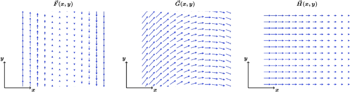

Tick whether the statement is true or false:
correct | incorrect | Response confidence | |||||||
a) | \(F_x = 0\) overall | [ ] | [ ] | very confident | [ ] | [ ] | [ ] | [ ] | not confident |
b) | \(F_y = 0\) overall | [ ] | [ ] | [ ] | [ ] | [ ] | [ ] | ||
c) | \(G_x = 0\) overall | [ ] | [ ] | [ ] | [ ] | [ ] | [ ] | ||
d) | \(G_y = 0\) overall | [ ] | [ ] | [ ] | [ ] | [ ] | [ ] | ||
e) | \(H_x = 0\) overall | [ ] | [ ] | [ ] | [ ] | [ ] | [ ] | ||
f) | \(H_y = 0\) overall | [ ] | [ ] | [ ] | [ ] | [ ] | [ ] | ||
-
II)
Given three vectors in the x-y plane. Sketch the vector component decomposition in x- and in y-direction:
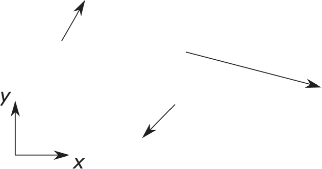

Rights and permissions
Open Access This article is licensed under a Creative Commons Attribution 4.0 International License, which permits use, sharing, adaptation, distribution and reproduction in any medium or format, as long as you give appropriate credit to the original author(s) and the source, provide a link to the Creative Commons licence, and indicate if changes were made. The images or other third party material in this article are included in the article’s Creative Commons licence, unless indicated otherwise in a credit line to the material. If material is not included in the article’s Creative Commons licence and your intended use is not permitted by statutory regulation or exceeds the permitted use, you will need to obtain permission directly from the copyright holder. To view a copy of this licence, visit http://creativecommons.org/licenses/by/4.0/.
About this article

Cite this article
Hahn, L., Klein, P. Clustering eye-movement data uncovers students’ strategies for coordinating equations and diagrams of vector fields. Educ Stud Math (2023). https://doi.org/10.1007/s10649-023-10243-y
Accepted:
Published:
DOI: https://doi.org/10.1007/s10649-023-10243-y