Dry granular masses impacting on rigid obstacles: numerical analysis and theoretical modelling

Abstract

The assessment of the time evolution of the impact force exerted by dry flowing masses on rigid obstacles is mandatory for the dynamic design of sheltering structures and the evaluation of the vulnerability of existing structures. In this paper, the results of an extensive numerical campaign performed by employing a discrete element method (DEM) code are presented and the role of different geometrical factors (flow length, height and front inclination) and state parameters (porosity and velocity) on the impact force–time evolution is investigated. The impact process is studied to correlate local information with the macroscopic response and a physically based force–time function, generalising the formula already introduced by the authors for the assessment of maximum impact force, in which each parameter is correlated with the previously mentioned factors, is proposed.

1 Introduction

Flow-like landslides represent a dangerous geological hazard occurring in mountain territories all around the world [32]. To this category, ranging from dry debris flows to rock avalanches, rapid movements of granular materials containing a large amount of gravel and rock fragments belong. Due to the huge volumes and high velocities, dry flows can pose significant hazard to human lives and cause significant damages to buildings and infrastructures [41].

To mitigate the risk associated with this kind of hazardous phenomena, structural protection measures are usually designed in landslide prone areas, to stop, intercept or slow down the flow [31].

In most national standards, [42, 65, 66] technical guidelines [21, 24, 25, 42] and scientific reports [40], the design of sheltering structures is mainly based on the pseudo-static approach where the maximum value of the impact force is statically applied to the barrier. In this case, the maximum impact force represents the most relevant input variable and is assumed to depend on flow height, front inclination and impact velocity [12]. Its evaluation is derived from empirical formulae inspired to hydrostatic [4, 31, 34, 66], hydrodynamic [3, 4, 21, 31, 42, 66], hybrid [3, 20] or boulder impact theories [21, 30, 40, 42], based on oversimplifying hypotheses about the behaviour of the granular material and on the use of highly dispersed empirical coefficients calibrated on real cases data [11].

As is well known, the use of pseudo-static approaches is too conservative and, nowadays, displacement-based design is preferred. This makes necessary, under the assumption of uncoupling the analysis of the sheltering structure from the simulation of the flowing mass propagation, the definition of the impact force temporal evolution and this is the final goal of this paper.

In the literature, the methods employed to evaluate the impact force and study the dynamic interaction between the granular mass and the obstacle are based on (i) historical cases, (ii) real and small-scale flume tests and (iii) numerical analyses.

(i) Impact forces recorded after real debris flow events are reported, for example, in Zhang [71] and Hu et al. [29], whereas real-scale experiments have been carried out by Bugnion et al. [9]. These tests are characterised by huge costs and efforts in the device installation and operations. Nevertheless, the impact flow geometry and kinematics cannot be precisely defined.

(ii) Small-scale flume tests have been performed all around the world in the last forty years and represent a very diffuse alternative for studying flow–barrier interaction [1, 14, 16, 17, 38, 39, 50,51,52, 55, 62, 64, 68]. These experimental test results provide information on some factors affecting the temporal evolution of the impact force, such as the mean value of the front velocity and flow height. These studies have shown that the impact is essentially dominated by the flow regime, in particular by the ratio of inertial to gravitational forces, which is conveniently described by Froude number, F_r [5, 16, 31, 37].

What is unfortunately absent in small-scale studies is a detailed description, useful for validating numerical simulations, of both flow kinematics (velocity profile), mass density and front geometry.

Moreover, due to the very small soil volumes employed, while the maximum impact force can be easily measured, obtaining realistic values of the impact force–time evolution it is very difficult, since the impacting mass is extremely short and the Froude numbers are above the typical real case values [62].

(iii) In recent years, numerical methods, capable of dealing with large displacements and simulating soil–structure interactions, have been developed. Some methods are based on continuum mechanics, adopting a Eulerian [50] integration strategy, hybrid Eulerian/Lagrangian techniques [15, 45,46,47] or meshless methods [28]. Nevertheless, these methods appear to be not sufficient to accurately reproduce the obstacle–flow interaction, where sudden changes in field variables, large deformation, intensive compaction and high strain rates occur. Continuum methods should require advanced constitutive models accounting for the dependence of the material response on grain packing and strain rate [15, 56, 57, 69].

Discrete methods, (DEM) [18], have been widely used to model and quantify the dynamic interaction between dry masses and obstacles [2, 12, 13, 17, 43, 44, 49, 63, 67, 70]. DEM allows to take natively into account large displacements, energy transformation, local variation of porosity and internal microstructure evolution, as well as to describe the dissipation mechanisms characterising the granular material in both frictional and collisional regimes [59].

To better understand the impact mechanics, very recently, the authors have published different works presenting the results of an extensive numerical campaign performed by using a discrete element 3D model [11,12,13, 15, 58]. The approach consists in generating the granular mass just in front of the obstacle, and the velocity is assigned as initial condition. The role of granular temperature/velocity fluctuations, although the authors are perfectly aware of its importance [56, 59], for the sake of simplicity, is disregarded. Such an approach allows to investigate separately the role of each geometrical factor (length, flow height, front inclination) and state parameters (porosity and velocity) [12, 13] and to better interpret the numerical results. On the negative side, the impact initial conditions may seem somehow independent and artificial, since they are not the outcome of a run-out simulation performed on the same material. In Calvetti et al. [12] the results have been interpreted from a macroscopic point of view in terms of maximum impact force and a new design formula has been introduced. Several design factors determining the impact force, namely the geometry of the sliding mass (length, width and flow height, inclination of the front) and the impact velocity, have been considered. In Calvetti et al. [11], the previous numerical results, have been compared with the most common approaches and empirical formulas available in the literature, as inferred either from small-scale flume tests or field measurements. Calvetti et al. [13] investigated the impact phenomenon from a micromechanical point of view, by correlating both particles kinematics and contact forces distribution as well as the evolution of the energy contents, with the observed macroscopic response, in particular during the first-time instants of the impact.

By employing the same numerical model, this paper focuses on an unexplored aspect that is the time evolution of the impact force.

The interaction mechanisms governing the phenomenon, from the impact inception until the complete arrest of the mass, are investigated. The DEM model allows (i) to obtain a data set, previously not available in the literature, highlighting the effect of the initial conditions on the shape of the force–time curve and (ii) to provide a more comprehensive framework, useful for critically interpreting experimental data.

In this paper, the investigated range of parameters is based on data reported in the literature for real debris flow events [9, 19, 36, 54, 60] in terms of average impact velocity, mass porosity, front inclination and flow height. All the considered impacts are characterised by Froude numbers ranging from 0 to 3, consistent with those estimated for most common real-scale observations [16, 31, 62].

Following the same line proposed in Calvetti et al. [12] for the maximum impact force, a parametric formula describing the time evolution of the impact force as a function of input data is also introduced.

The paper is organised as follows: in Sect. 2, the DEM numerical model, the micromechanical parameters and the imposed initial conditions are detailed. In Sect. 3, the DEM numerical results are analysed and critically discussed to highlight the physical and mechanical processes responsible for the macromechanical response. In Sect. 4 a comprehensive formula for simulating the force–time evolution, based on the previously described mechanical interpretation of the impact process, is proposed.

2 DEM model

DEM analyses have been performed by using code PFC3D [35] where the original DEM formulation of Cundall and Strack [18] is implemented.

The DEM model, which has been validated by reproducing the experimental test result of Jiang and Towhata [38], is analogous to that described in [11,12,13, 15, 58].

The impacting dry soil mass is simulated as an assembly of polydispersed spherical particles of density ρ_s with a uniform diameter distribution ranging between $D_{\max }$ and $D_{\min }$ and average grain diameter D. The boundary and the obstacle are described as rigid wall elements.

Grain–grain and grain–wall local interactions are governed by normal and tangential contact stiffnesses (k_n and k_s) and contact friction (μ_s). As in Calvetti et al. [12, 13] and Ceccato et al. [15], the mechanical response of a real granular material, with rough and angular grains, is reproduced by inhibiting particle rotations [10, 67]. The authors have previously performed some analyses not inhibiting grain rotations [15] and did not observed significant quantitative differences in the dynamic contribution of the impact force. In fact, since the material is loose and flowing under very large velocities, shear localisation phenomena do not occur. Similar results could be obtained using irregular clumps instead of spheres, as was shown in Albaba et al. [2].

The choice of micromechanical parameters (Table 1) is based on the calibration procedure reported in Calvetti [10], where the ranges of model parameters to be used for simulating the response of a sand are provided, based on the reproduction of triaxial compression experiments. The authors have performed triaxial tests by employing the parameters reported in Table 1 (not reported for the sake of brevity) and obtained a response analogous to that obtained by Calvetti [10]. In particular, the residual friction angle is equal to ϕ′ = 36° and the critical state porosity n_cr = 0.416.

Table 1 List of micromechanical parameters

No contact damping is used.

The model geometry and the initial conditions are illustrated in Fig. 1.

Fig. 1

3D view of the DEM model

Simulations are performed under plane-strain conditions: the dry granular mass is confined between two lateral smooth and rigid wall elements. Basing on preliminary sensitivity analyses, in order to prevent boundary effects, [12, 13, 15], the channel width b is imposed equal to 8 D.

The base wall is characterised by a friction coefficient μ_b. The obstacle is modelled as a vertical rigid wall of height H and friction coefficient μ_w. As shown in Ceccato et al. [15], the value of wall friction does not affect the impact force value.

The geometry of the impacting mass is characterised by a length L, height h₀, front inclination α₀, initial velocity u₀ and porosity n₀.

The results of the sensitivity analyses aimed at investigating the influence of D/h₀ and $D_{\max } /D_{\min }$ on numerical results are reported in Appendix D. The authors have shown that, in agreement also with the results of Ceccato et al. [15] and Cui et al. [17], by imposing D/h₀ ≤ 0.067, the number of particles is large enough to obtain both sufficiently accurate description of the problem and a reasonable computational time (Fig. 27). Moreover, the effect of $D_{\max } /D_{\min }$ on the temporal evolution of impact force is negligible (Fig. 28).

The influence of the input parameters was analysed by performing several tests for different combinations of initial conditions (Table 2). The range of investigated impact conditions is consistent with data concerning real-scale phenomena [9, 16, 19, 36, 53, 54, 60]. Among the 80 numerical tests performed, only 19 tests are described in detail in the following sections. The relative geometrical parameters and initial conditions are reported in Table 3.

Table 2 Model data and test conditions (the values between brackets refer to the test used for reference, Test 1 of Table 3)

Table 3 DEM tests: geometrical parameters and initial conditions imposed

The same simulation procedure employed by Calvetti et al. [12, 13] has been adopted: (i) initially, the dry granular mass is generated under zero gravity conditions. In this stage, particles are frictionless and the mass is free from contact forces; (ii) interparticle friction $\mu_{s}$, gravity and initial impact horizontal velocity $u_{0}$ are assigned to all particles; (iii) the impact is simulated and the evolution of the horizontal component of the impact force is monitored over time.

3 DEM results

In this section, the DEM numerical results are discussed to correlate the phenomena occurring within the granular mass during the impact process with the time evolution of the impact force.

In Sect. 3.1 a reference impact is studied, whereas in Sect. 3.2, the role of each initial condition and geometrical parameter in affecting the dynamic phenomenon is analysed.

3.1 The reference impact

In this paragraph, the reference impact test (Test 1 of Table 3), characterised by α₀ = 60°, n₀ = 0.45, L = 60 m and u₀ = 8 m/s, is considered.

The force–time curve plotted in Fig. 2 is characterised by an initial pseudo-linear increase until a first peak force, f_p, is attained at t = t_p. Then, the response presents a quite irregular trend, characterised by numerous sub-peaks with oscillations of rather constant period and progressively decreasing amplitude. When oscillations nullify, the curve converges to a final constant residual value f_res. As is shown here in the following, the shape of the force–time curve is mainly affected by three distinct phenomena:

• I. the evolution of the contact height;

• II. the compression and rarefaction waves propagation;

• III. the progressive arrest of the mass in front of the obstacle.

Fig. 2

DEM numerical results (Test 1): time evolution of impact force

3.1.1 Evolution of contact height

As is evident in Fig. 3, the contact height h between the mass and the obstacle evolves with time $t$ during the impact process. h initially increases about linearly, while the geometry of the front progressively flattens and part of the mass piles up behind the obstacle forming a triangular dead zone already observed by Calvetti et al. [13]. At $t = \overline{t}$ (0.21 s in this case) h reaches the flow height $h_{0}$. The linear increase in h for $t < \overline{t}$ is related with the planar shape of the flow front (Fig. 4):

$$h\left( t \right) = u_{0} \cdot \tan \alpha_{0} \cdot t,$$

(1)

from which:

$$\overline{t} = \frac{{h_{0} }}{{u_{0} \tan \alpha_{0} }}.$$

(2)

Fig. 3

Evolution of the contact height (reference impact)

Fig. 4

Schematic representation of the geometry evolution of the flow front for $t < \overline{t}$

For $t > \overline{t}$, the incoming material flows along the surface of the dead zone, particles are deflected upwards [13] and h continues to increase, although more slowly, from $h_{0}$ to the final value h_res (4.95 m). This process was also observed by Jiang et al. [39], and Ng et al. [51] in experimental flume tests and by Xiao et al. [70], Shen et al. [63] in DEM simulations.

3.1.2 Compression and rarefaction waves propagation

As was observed by Calvetti et al. [13], Ceccato et al. [15] and Federico and Amoruso [22] using DEM, material point method (MPM) and finite element method (FEM) respectively, during the impact process when the mass hits the obstacle, a compression wave, generated at the mass front, travels backwards within the granular material with velocity u_m, creating highly loaded horizontal force chains.

At the first peak time t_p, the dynamically created compressive force chains become unstable, this resulting in force chains disruption. This process, which is analogous to the typical buckling phenomenon [13, 15], produces the onset of a sort of rarefaction wave propagating from the surface toward the bed with velocity u_f, and the impact force drops (Fig. 2).

According to FEM and MPM analyses, based on a continuum approach, the rarefaction wave velocity depends uniquely on density and coincides with u_m, while DEM simulations show that u_r decreases with both Froude number (Fig. 14) and porosity [58].

To better interpret the trend characterising the force–time curve, in Fig. 5, four numerical test results are compared (α₀ = 90° and 60°; confined and unconfined flow). The confined flow represents an ideal condition which is obtained by adding a horizontal wall at the top of the mass. For both front inclinations, the initial behaviour (i.e., $t < t_{p}$) is unaffected by the confinement condition.

Fig. 5

Impact force evolution: confined and unconfined flow, vertical and inclined front

As observed by Calvetti et al. [13] in case of vertical front, if the flow is confined, the impact process resembles that of a solid body impacting on a rigid wall and the force value, that is almost constant, is approximately equal to that calculated by employing the linear impulse theory $f = \rho \cdot u_{0} \cdot u_{m} \cdot h_{0}$. The compression wave velocity u_m can be easily numerically assessed under confined conditions as described in Calvetti et al. [12, 13] and Redaelli et al. [58] and, in case of n₀ = 0,45, u_m = 160 m/s.

In contrast, under unconfined conditions, the impact force drops at $t_{p}$ due to the buckling process.

In case of inclined fronts, if the flow is confined, the force continues to increase about linearly until $t = \overline{t}$ (i.e. when the contact height attains h₀) getting a force value practically coincident with that obtained for α₀ = 90°. In the unconfined case (reference impact), the impact force starts decreasing when $t > t_{p}$, which is significantly smaller than $\overline{t}$. In other terms, as is shown in Fig. 3 and in agreement with Calvetti et al. [12] and Ceccato et al. [15], the peak occurs when the contact height is smaller than the flow height ($h\left( {t_{p} } \right) \le h_{0} )$.

After the buckling phase contact forces can regenerate due to the pressure exerted by the material flowing behind the dead zone. The successive oscillations characterising the force–time curve (Fig. 2) are thus associated with a continuous regeneration (compression wave) and disruption (due to total or partial buckling) of the force chains network in the granular mass and are signature of the hybrid solid/fluid nature of the granular material [13, 51, 59].

3.1.3 Progressive arrest of the mass in front of the obstacle

During the impact process, the dead zone progressively extends backwards. As was observed by Shen et al. [63], Luo and Zhang [48], Xiao et al. [70], the increase in the dead zone thickness justifies the attenuation of subsequent impacts and the reduction of the force oscillation amplitude. When the final geometry of the deposit is attained, the residual force $f_{res}$ is obtained (425 kN/m for Test 1) (Fig. 2).

The trust coefficient $k_{res}^{*}$ is defined as the ratio of $f_{res}$ to the hydrostatic pressure

$$k_{{{\text{res}}}}^{*} = \frac{{f_{{{\text{res}}}} }}{{\frac{1}{2}\rho \cdot g \cdot h_{{{\text{res}}}}^{2} }},$$

(3)

being $\rho = \rho_{s} \left( {1 - n_{0} } \right)$ the mass density and g the gravity acceleration. For Test 1, $k_{{{\text{res}}}}^{*} = 2.47$, which is between the value of the active and passive trust coefficients (k_a = 0.26 and k_p = 3.85), calculated by assuming a critical state friction angle of 36° for the granular mass (Sect. 2).

3.2 Parametric analyses

In Fig. 6, the effect of initial velocity $u_{0}$, initial porosity $n_{0}$, flow height $h_{0}$, front inclination $\alpha_{0}$ and flow length $L$ on the impact force evolution is summarised.

Fig. 6

Impact force–time evolution for different a initial velocities, b initial porosities, c flow heights, d front inclinations and e flow lengths

The role of impact velocity is particularly relevant both quantitatively and qualitatively (Fig. 6a): for decreasing $u_{0}$, the maximum impact force strongly reduces, the peak time instant increases and both impact duration and residual force decrease. For low values of $u_{0}$, the oscillations progressively disappear and the difference between the maximum impact force and the residual force becomes negligible.

Maximum impact force, peak time and the residual force slightly decrease with $n_{0}$ (Fig. 6b); on the contrary, the amplitude of oscillations increases with $n_{0}$.

In Fig. 6b, both porosity and state parameter ${\Psi }_{0} = n_{0} - n_{cr}$ [7] are given, where $n_{cr}$ is the porosity at critical state corresponding to the atmospheric pressure. ${\Psi }_{0}$ is the most important parameter governing the material response [69]. In a flowing material, ${\Psi }_{0}$ is usually positive and tends to increase with flowing velocity [56, 59]. For this reason, in the following, the authors decided to impose as reference porosity $n_{0}$ = 0.45, which is above the critical value for the considered grain size distribution ($n_{cr}$ = 0.416). Larger values are not considered since the response of the materials would be more similar to that of a granular gas, without contacts among particles [58], conditions typical of granular materials with not realistic flowing velocities. An extensive study on the role of initial porosity is in Redaelli et al. [58].

The flow height has a strong influence on the overall evolution of the impact force (Fig. 6c). In particular, as $h_{0}$ increases, maximum impact force, peak time, oscillation amplitude period and residual force markedly increase, whereas the initial slope of the force–time curve does not change.

The front inclination has a large influence on the initial evolution of the impact force (Fig. 6d). In fact, both maximum impact force and initial curve slope increase with α₀. For large front inclinations, the first peak is attained very rapidly (virtually immediately for α₀ = 90°) and is much higher than the following peaks. However, all curves converge with time to a common trend, characterised by the same oscillation amplitude and residual force.

As is evident in Fig. 6e, both maximum impact force and peak time are not influenced by the flow length. On the contrary, the evolution with time of the impact force is severely influenced by L: (i) in case of sufficiently short masses, the post peak oscillations tend to disappear (as is typically observed in flume experimental tests), (ii) both residual force and impact duration increase with L, although this dependency vanishes for L sufficiently large (L > 30 m). In the paper, sufficiently long masses ($L/h_{0}$ > 20) will be considered and the effect of L on the residual force will be neglected.

Here below, the role of initial conditions on the three processes already discussed in Sect. 3.1 is studied.

3.2.1 Evolution of contact height

In Fig. 7, the evolution with time of the normalised contact height $h^{*} = h/h_{0}$ is plotted for impacts characterised by different velocities (Fig. 7a), heights (Fig. 7b) and front inclinations (Fig. 7c).

Fig. 7

Evolution of normalised contact height for different a initial velocities; b flow heights; c front inclinations

From a qualitative point of view, all graphs share a similar trend. Both initial slope and final value $h_{{{\text{res}}}}^{*} = h_{{{\text{res}}}} /h_{0}$ increase with $u_{0}$ (Fig. 7a) and decrease with $h_{0}$ (Fig. 7b). For low impact velocities ($u_{0}$ = 2 m/s in this case), $h_{{{\text{res}}}}^{*}$ does not reach 1: the mass stops before the complete flattening of the front. The initial slope increases also with front inclination (Fig. 7c). The final value $h_{{{\text{res}}}}^{*}$ is barely affected by $\alpha_{0}$. Note that for $\alpha_{0}$ = 90°, $h^{*} = 1$ at $t = 0$.

The geometry of the deposit (residual state) is plotted in Fig. 8 for different Froude numbers $F_{r0}$, being

$$F_{r0} = \frac{{u_{0} }}{{\sqrt {g \cdot h_{0} } }},$$

(4)

[5, 16, 31, 37], and two different front inclinations. In Fig. 9, the normalised residual height $h_{{{\text{res}}}}^{*}$, is plotted as a function of $F_{r0}$ for different front inclinations.

Fig. 8

Deposit geometry with contact forces for different Froude numbers and front inclinations

Fig. 9

Normalised residual height versus Froude number for different front inclinations

From these results it is possible to conclude that:

• $h_{res}^{*}$ increases with $F_{r0}$;

• when $F_{r0}$ < 1, $h_{res}^{*}$ depends on $\alpha_{0}$, in particular, for $F_{r0} \to 0$ and $\alpha_{0}$ = 90°, $h_{res}^{*} \to 1$ whereas when $\alpha_{0}$ < 40°, $h_{res}^{*} \to 0$;

• for $F_{r0}$ sufficiently high ($F_{r0} > 1)$, $h_{res}^{*}$ barely depends on $\alpha_{0}$.

3.2.2 Compression and rarefaction waves propagation

In this section, the effect of initial conditions on the oscillatory trend of the force–time curve is investigated.

In Fig. 10, the first peak time $t_{p}$ is plotted as a function of $h_{0}$, $u_{0}$ and $\alpha_{0}$: (i) $t_{p}$ linearly increases with $h_{0}$ (Fig. 10a), (ii) $t_{p}$ decreases with $u_{0}$ approaching the limit $t_{p} =$ 0 for sufficiently large $u_{0}$ values (Fig. 10b), (iii) $t_{p}$ decreases with $\alpha_{0}$ and $t_{p} =$ 0 in case $\alpha_{0} =$ 90° (Fig. 10c). This implies that the dependence of $t_{p}$ on $h_{0}$, $u_{0}$ and $\alpha_{0}$ is analogous to that one given in Eq. 2 for $\overline{t}$.

Fig. 10

Peak time as a function of a flow height, b flow velocity and c front inclination

The analysis of the numerical data allows the authors to state that the ratio $t_{p} /\overline{t}$ is not affected by $F_{r0}$ but depends on the material porosity/deformability. To emphasise it, in Fig. 11$t_{p} /\overline{t}$ is plotted for two different values of $u_{0}$, $h_{0}$, and $\alpha_{0}$ = 40–60° and two values of state parameter ${\Psi }_{0}$, one positive and one negative: although a certain dispersion of data is observed, $t_{p} /\overline{t}$ tends to increase with ${\Psi }_{0}$.

Fig. 11

$t_{p} /\overline{t}$ versus state parameter

The effect of initial conditions on buckling is illustrated in Fig. 12, where the evolution of the normalised impact force $f/f_{p}$ and of the coordination number Z (average number of contacts per particle within a spherical domain of radius 1.4 m and placed at a distance equal to 1.5 m from the obstacle) is plotted for various front inclinations and impact velocities.

Fig. 12

Influence of impact velocity (α₀ = 90°) (a–b) and front inclination (u₀ = 8 m/s) (c–d) on the time evolution of $f/f_{p}$ and Z

In case of $\alpha_{0} \ge$ 80° and larger impact velocities ($u_{0} \ge$ 8 m/s), after the peak, both the normalised impact force and coordination number decrease very rapidly to zero (Fig. 12a) and remain zero for a long time, signature that the contact network is completely disrupted [59].

As was observed by Calvetti et al. [13], in this phase rarefaction has involved the entire thickness of the stratum. The material has virtually liquefied: vertical velocities of particles are predominant with respect to horizontal and a jet-like phenomenon tends to occur.

The buckling phenomenon tends to reduce for decreasing impact velocities and front inclinations (Fig. 12c, d). For $u_{0} <$ 8 m/s and $\alpha_{0} \le$ 60° neither the impact force nor the coordination number nullify signature that the disruption of force chains is partial.

Buckling tends to reduce in the secondary oscillations, as is evident in Fig. 13, where the trend of the coordination number is plotted for impacts characterised by different $u_{0}$ values. Both Z, at $t = t_{p}$, and the amplitude of its oscillations increases with $u_{0}$. If $u_{0}$ is sufficiently low ($u_{0}$ = 2 m/s), the fluctuations are negligible.

Fig. 13

Time evolution of the coordination number

In all impacts, after the first peak, impact force oscillations reach a regime condition characterised by a period $T$ (Fig. 6), related to the time employed to generate (compression wave) and erase (rarefaction wave) the force chains network. As was already observed, $T$ increases with both $u_{0}$ (Fig. 6a) and $h_{0}$ (Fig. 6c). The counter-intuitive influence of impact velocity is justified by the disruptive effect of buckling that increases with $u_{0}$. To quantitatively interpret this evidence, the quantity $u_{r} = h_{0} /\left( \frac{T}{2} \right)$ is introduced. $u_{r}$ can be interpreted as the velocity of the rarefaction wave, travelling the distance $h_{0}$ to fully nullify the contact forces, which occurs in half of the oscillation period. As is shown in Fig. 14, $u_{r}$ is a decreasing function of F_r0 and is not affected by front inclination.

Fig. 14

Rarefaction wave velocity versus Froude number

3.2.3 Progressive arrest of the mass in front of the obstacle

Due to the progressive dissipation of kinetic energy, the impact force oscillations gradually disappear and the impact force gets its residual value $f_{{{\text{res}}}}$. As was already discussed, $f_{{{\text{res}}}}$ mainly depends on $u_{0}$, $h_{0}$ and L.

Several literature contributions discuss whether the residual earth pressure is close to either active or passive conditions [48]. Some authors suggest that the residual force is equal to passive thrust, since the material is in a compressive state [19, 39, 50]. However, other authors observe that the residual earth pressure ranges between the active and passive one [51, 52].

To discuss this issue, in Fig. 15a, the thrust coefficient $k_{{{\text{res}}}}^{*}$ (Eq. 4) is plotted as a function of $F_{r0}$. The dashed lines in Fig. 15a represent the passive and active thrust coefficients, $k_{p}$ and $k_{a}$, respectively. It is evident that:

• for nullifying values of $F_{r0}$ (quasi-static flow), $k_{{{\text{res}}}}^{*}$ tends to $k_{a}$;

• for $0.4 < F_{r0} < 1$, $k_{{{\text{res}}}}^{*}$ remains approximately constant and close to the passive thrust coefficient;

• for $F_{r0} > 1$, $k_{{{\text{res}}}}^{*}$ decreases and approaches the unit value for sufficiently large $F_{r0}$ values. In this limit case, the response of the material is more similar to that of a fluid at rest in which the state of stress is approximately isotropic [59].

Fig. 15

Thrust coefficient under residual conditions: a influence of front inclination and Froude number; b influence of Froude number and $L/h_{0}$

The influence of $F_{r0}$ and ratio $L/h_{0}$, on thrust coefficient $k_{res}^{*}$ is illustrated if Fig. 15b. For small $L/h_{0}$ values, $k_{res}^{*}$ increases. For $L/h_{0}$ sufficiently high, a plateau is reached. The value of $L/h_{0}$ above which the thrust coefficient is constant increases with $F_{r0}$. For all $F_{r0}$ values, in case $L/h_{0} > 20$ the trust coefficient is constant.

4 Impact loading function

In this section, the authors provide an impact force–time function to be employed for design purposes and they discuss the validity domain of the formula. Since the obstacle is assumed to be rigid, the formula provides an upper bound for impact force.

4.1 Analytical expression

The design function suggested here below stems from the physical and mechanical interpretation of the numerical DEM results of Sect. 3 and represents an improvement of the formula previously defined by the authors [12] for the maximum impact force.

For the sake of generality, the impact force function is expressed in non-dimensional terms by introducing the following quantities:

$$f^{*} = \frac{f}{{\frac{1}{2} \cdot \rho \cdot g \cdot h_{0}^{2} }},$$

(5)

$$t^{*} = \frac{t}{T},$$

(6)

being $T = 2h_{0} /u_{r}$ the previously defined period (Fig. 14). $u_{r}$ can be calculated by using the interpolation function $u_{r} = u_{r} \left( {F_{r0} } \right)$, given in Appendix B (Eq. 20).

The analysis of the numerical simulations suggests $f^{*}$ to be expressed as a linear combination of an inertial force $f_{i}^{*}$, associated with the integral of a uniform horizontal pressure distribution, and a residual force $f_{{{\text{res}}}}^{*}$, corresponding to the integral of a linear pressure distribution:

$$f^{*} \left( {t^{*} } \right) = f_{i}^{*} \left( {t^{*} } \right) \cdot \xi \left( {t^{*} } \right) + f_{{{\text{res}}}}^{*} \cdot \left( {1 - \xi \left( {t^{*} } \right)} \right),$$

(7)

where $\xi \left( {t^{*} } \right)$ is a decay function describing the decay of kinetic energy: $\xi \left( {t^{*} = 0} \right) = 1$ and $\xi (t^{*} \to \infty$) = 0. The role of $\xi \left( {t^{*} } \right)$ is to progressively reduce the inertial force contribution in favour of the residual one.

• I. Residual force contribution

  The residual force, that is the integral of the linear pressure distribution exerted by the mass at rest in front of the obstacle, can be written as:

  $$f_{{{\text{res}}}}^{*} = k_{{{\text{res}}}}^{*} \cdot h_{{{\text{res}}}}^{*2} ,$$

  (8)

  The values of $h_{{{\text{res}}}}^{*}$ and $k_{{{\text{res}}}}^{*}$ are calculated by using the interpolation functions $h_{{{\text{res}}}}^{*} = h_{{{\text{res}}}}^{*} \left( {F_{r0} ,\alpha_{0} } \right)$ and $k_{{{\text{res}}}}^{*} = k_{{{\text{res}}}}^{*} \left( {F_{r0} } \right),$ given in Appendix A (Eqs. 13, 15, respectively), derived from Figs. 9 and 15a, respectively. The reliability of Eq. 8 is confirmed by Fig. 16 where DEM data are compared with interpolating results in terms of residual force.

  Fig. 16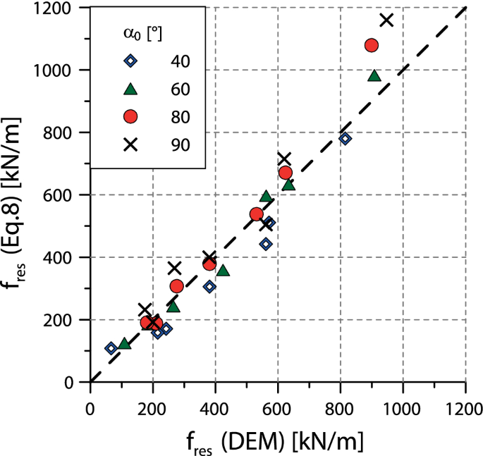

  

  Comparison with measured and computed residual force

• II. Inertial force contribution

  The simultaneous propagation of compressive and rarefaction waves during the impact process suggests the use of the following expression for the inertial force contribution:

  $$f_{i}^{*} \left( t \right) = \frac{1}{1-n_0} \cdot F_{r0} \cdot F_{{r,u_{m} }} \cdot h^{*} \left( {t^{*} } \right) \cdot \left\{ {1 - \sin^{2} \left[ {\pi \left( {t^{*} - t_{p}^{*} } \right)} \right]} \right\},$$

  (9)

  where.

  • $F_{{r,u_{m} }}$ is the intrinsic Froude number [12], defined as:

    $$F_{{r,u_{m} }} = \frac{{u_{m} }}{{\sqrt {gh} }},$$

    (10)

    being $u_{m}$ the compression wave velocity within the frictional mass (Sect. 3.1.2) [13].

  • $t_{p}^{*}$ is the non-dimensional peak time, introducing a phase shift in the oscillatory response (Sect. 3.1):

    $$t_{p}^{*} = \frac{{\overline{t}}}{T} \cdot c_{n} = \overline{t}^{*} \cdot c_{n} ,$$

    (11)

    where $\overline{t}$ is calculated according to Eq. 2 and $c_{n}$ is calculated by using the interpolation functions $c_{n} = c_{n} \left( {{\Psi }_{0} } \right)$ given in Appendix B, deriving from Fig. 11 (Eq. 16). For $\alpha_{0}$ = 90°, both $\overline{t}$ and $t_{p}^{*}$ tend to zero. The accuracy of the analytical expressions for the peak time (Eq. 11) is testified by Fig. 17 where the dimensional numerical and calculated data are compared.

  • $h^{*} \left( {t^{*} } \right)$ provides the evolution of the contact height with time, according to the trends reported in Fig. 7. Its expression, depending on both $h_{res}^{*}$ and $\overline{t}^{*}$, is reported in Appendix B (Eq. 17).

    Fig. 17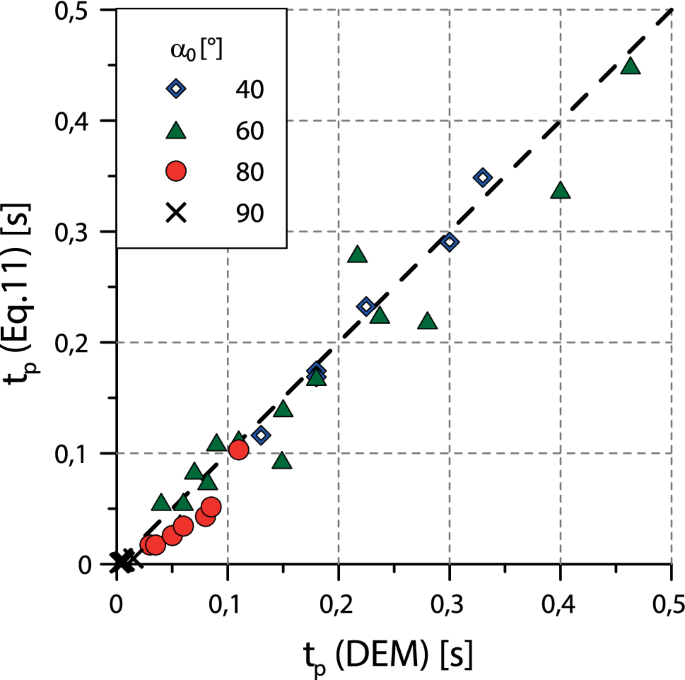

    

    Comparison with measured and computed peak time

The first term in Eq. 9 refers to the deformable solid body and derives from the linear impulse theory, whereas the second term is associated with the propagation of the rarefaction wave and defines the oscillating trend over time.

As $F_{r0}$ decreases, the oscillation period tends to zero (Fig. 14) and the second term in Eq. 9 vanishes. In this limit case, Eq. 9 reduces to the formula of the elastic body model (Sect. 3.1.2) [10].

• III. Decay function

  The following expression has been assumed for $\xi \left( {t^{*} } \right):$

  $$\xi \left( {t^{*} } \right) = e^{{ - c_{2} \cdot \left( {t^{*} } \right)^{{c_{1} }} }} ,$$

  (12)

  where $c_{1}$ and $c_{2}$ are non-dimensional coefficients which have been determined by interpolating the DEM impact force–time curve with Eq. 7 (Appendix C). $c_{1}$ (Eq. 21) regulates the shape of the decay curve, decreasing with both $F_{r0}$ and $\alpha_{0}$, whereas $c_{2}$ (Eq. 23) governs the speed of decay and increases with both $F_{r0}$ and $\alpha_{0}$.

In Fig. 18, the DEM force–time curve relative to the reference impact (Test 1) is compared with Eq. 7.

Fig. 18

Force–time curves for the reference impact (Test 1): numerical DEM results and proposed impact loading function

The dotted line, coinciding with the upper envelope of the force–time trend, corresponds to Eq. 7 without oscillations, whereas the dashed line, coinciding with the lower envelope, corresponds to the quasi-static contribution of Eq. 7. The good agreement between the numerical DEM data and the proposed impact loading function is evident. Differently to DEM simulations, the force computed by using the formula presents a second peak that is larger than the first peak. To explain this discrepancy, it is worth observing that, in DEM simulations, when the rarefaction wave propagates downward, the contact force chains network is completely disrupted and the re-solidification time of the material is a function of the kinetic energy and of the capability of the material of dissipating it (Sect. 3.2.2). In case of large initial kinetic energies, this effect is so destructive that the material struggles in dissipating the kinetic energy and regenerating the force chains network. This phenomenon, that is even amplified by the absence of contact viscous damping, is not taken into account by the analytical formula.

In Fig. 19 the DEM data discussed in Sect. 3.2 are compared with the impact loading function (Eq. 7) for different values of flow height (Fig. 19a, b) front inclination (Fig. 19c, d) and initial velocity (Fig. 19d, e). It is evident that the proposed formula, is capable of capturing both quantitatively and qualitatively the force–time evolutions, and of taking into account the dependence of the impact force on impact velocity, flow height and front inclination. The previously mentioned discrepancy tends to disappear when the impacting mass is characterised by a sufficiently small kinetic energy (small initial velocity or flow thickness) and the accordance between DEM results and analytical formula is excellent.

Fig. 19

Time evolution of the impact force: comparison between DEM data (left) and predictions obtained by using Eq. 7 (right) for different (a–b) initial velocities, (c–d) flow heights and (e–f) front inclinations

4.2 Validity domain

The impact loading function has been inferred from DEM numerical simulations and, for this reason, can be considered applicable within the validity domain defined by the ranges of initial conditions considered by the authors. The assumptions and the choices of input parameters are summarised here below.

All impacts are characterised by:

• $F_{r0} < 3$,

  consistent with those estimated for most common real-scale observations [16, 31, 62].

  Conversely, in small-scale tests, Froude numbers are above the typical real cases values [1, 39, 62]. Conversely, in small-scale tests, Froude numbers are above the typical real cases values [1, 39, 62].

• $\alpha \ge$ 40°.

  This constraint is reasonable for decelerating flowing masses as it happens when the mass is approaching the sheltering structure placed downstream. This also suggests that in small-scale flume tests, where smaller values of front inclinations are observed [1, 2, 50], the length of the channel is in general too short to achieve steady-state conditions and the mass is still accelerating.

• $\frac{L}{{h_{0} }} >$ 20.

  The authors have observed that, under this hypothesis, the evolution of the impact force is not affected by the length of the impacting mass (Fig. 15b). This information is of great importance since, in the literature, this parameter is usually disregarded in the impact force evaluation. In fact, in small-scale flume tests the ratio $\frac{L}{{h_{0} }}$ is in general too short [1, 2, 39, 50, 62], and, as a consequence, (i) the residual force is underestimated and (ii) force fluctuations are not observed.

• A uniform velocity and porosity profile.

  The velocity profile of the mass approaching the obstacle depends on the propagation phase and on boundary conditions. Experimental tests [6, 33, 39, 47, 61] have shown that this hypothesis is reasonable in case of masses flowing on a flat-frictional base, where the velocity profile tends to plug in the upper part, whereas a thin zone of higher shear is present close to the stationary surface. In case of extremely rough sliding surfaces, the velocity profile decreases gradually with depth and the hypothesis of uniform velocity profile is not realistic [8, 39]. In Appendix D, the authors have studied different impacts by imposing different velocity profiles (Fig. 29a) and observed that maximum impact force [12], first buckling, residual force and the impulse value are negligibly affected by the shape of the velocity profile (Fig. 29b,c).

• Dry masses with $D/h_{0} \le$ 0.067.

  Under this hypothesis, as shown by Cui et al. [17], particle size effects can be disregarded in the impact force assessment (Appendix D). But consequently, the formula is valid in case of impacts of dry debris flows but not in case of rock blocks avalanches.

  Within the validity domain, the formula can be easily employed by the designer, since all the coefficients are only function of the initial conditions at the pre-impact instant of time (namely initial Froude number and front inclination). The only parameter that is not directly provided is the compression wave velocity. Nevertheless, several empirical relationships are available in the literature to correlate relative density and the velocity of propagation of compression wave in porous media [26, 27].

5 Conclusions

In this paper, a discrete element method numerical code has been employed to study the dynamic interaction between a dry granular mass and a rigid obstacle. The impacting mass has been generated just in front of the obstacle at the pre-impact time instant. The DEM model proposed by the authors has allowed to obtain a data set, previously not available in the literature, highlighting the effect of the initial conditions (flow length, width and height, front inclination, impact velocity) on the temporal evolution of the impact force. Independently of initial conditions, the force–time curve exhibits a trend characterised by an initial increase in the impact force, until a first peak is attained, followed by different sub-peaks occurring with a precise oscillatory period and with a progressively decreasing amplitude, until a final constant residual value is got.

The mechanical and physical interpretation of the numerical DEM results put in evidence that (i) the granular mass involved in the impact process behaves like both a solid and a fluid material and (ii) the macroscopic response is governed by different concurring mechanisms: (a) the progressive increase in the contact height between the mass and the obstacle; (b) the propagation of both compression and rarefaction waves within the mass; and (c) the dissipation of the kinetic energy with a progressive arrest and pile-up of the mass behind the obstacle.

The numerical results obtained have allowed also to critically interpret the experimental data available in the literature. In fact, experimental tests are characterised by the lack a precise description of flow conditions, flow kinematics and front geometry. For example, the authors have discovered that the flow length $L$, that is in general neglected in most of the empirical formulae, is an important parameter influencing the shape of the force–time curve and the residual force value. For this reason, small-scale tests are useful to provide qualitative information about the most important parameters affecting the impact force but fails in providing a reliable input for a quantitative assessment of the impact force.

Starting from the physical–mechanical parametric analysis of the impact process, the authors have proposed an impact loading function that can be employed by designers since each parameter has been correlated with either the imposed initial conditions or the initial Froude number, quantifying the dynamicity of the impact process.

These initial conditions are assumed to be obtained as output of the propagation analysis that can be performed by employing numerical simulations either with depth averaged models or fully 3D analyses.

The formula is capable of capturing both qualitatively and quantitatively the numerical force–time evolution for many real cases situations and can be employed as an input loading function for the dynamic design of sheltering structures.

As a consequence, the results obtained in the paper would have a paramount impact in the design of rigid protection structures, overpassing the limitations of pseudo-static approaches.

Appendices

Appendix

Appendix A: Residual force contribution

In Eq. 8, $f_{{{\text{res}}}}^{*}$ is assumed to be a function of both $h_{{{\text{res}}}}^{*}$ and $k_{{{\text{res}}}}^{*}$.

Here below, the expression for $h_{{{\text{res}}}}^{*} = h_{{{\text{res}}}}^{*} \left( {\alpha_{0} ,F_{r0} } \right)$ and $k_{{{\text{res}}}}^{*} = k_{{{\text{res}}}}^{*} \left( {F_{r0} } \right)$ are given.

The DEM numerical data of Fig. 9 have been fitted (Fig. 20) by employing the following analytical expression:

$$h_{{{\text{res}}}}^{*} = \sqrt {F_{r0}^{2} + a_{1} } ,$$

(13)

where parameter $a_{1} = a_{1} \left( {\alpha_{0} } \right)$ is given by

$$a_{1} = 0.015 \cdot \alpha_{0} - 0.44,$$

(14)

with $\alpha_{0}$ expressed in degrees.

Fig. 20

Normalised residual height versus Froude number for different front inclinations: comparison between fitting curves (Eq. 13, dashed lines) and DEM data

Analogously, in Fig. 21 the comparison between DEM data of Fig. 15a and the following interpolating function is illustrated:

$$k_{res}^{*} = \left\{ {\begin{array}{*{20}l} {\frac{{k_{p} }}{0.41} \cdot F_{r0} } \hfill & {{\text{if}}\;F_{r0} < 0.41} \hfill \\ {k_{p} } \hfill & {{\text{if }}\;0.41 \le F_{r0} \le 1} \hfill \\ {1 + \left( {k_{p} - 1} \right) \cdot F_{r0}^{ - 2.5} } \hfill & {{\text{if}}\;F_{r0} > 1} \hfill \\ \end{array} } \right.$$

(15)

Fig. 21

Thrust coefficient versus Froude number and fitting curve (Eq. 15, dashed line)

Appendix B: Inertial force contribution

The expression for $c_{n} = c_{n} \left( {{\Psi }_{0} } \right)$, employed in Eq. 11 to assess the peak time, has been obtained by fitting the DEM numerical data of Fig. 11 with the following straight line (Fig. 22):

Fig. 22

Ratio coefficient $t_{p} /\overline{t}$ versus state parameter: comparison between DEM data (symbols) and fitting curve (Eq. 16, dashed line)

$$c_{n} = 3.5 \cdot {\Psi }_{0} + 0.3$$

(16)

The evolution with time of $h^{*}$ is described by using the following equation:

$$h^{*} \left( {t^{*} } \right) = \langle h_{{{\text{res}}}}^{*} - 1\rangle\left[ \langle{1 - \frac{{t^{*} }}{{\overline{t}^{*} }}\rangle\frac{{t^{*} }}{{\overline{t}^{*} }} + \langle\frac{{t^{*} }}{{\overline{t}^{*} }} - 1\rangle\left( {h_{{{\text{res}}}}^{*} - \left( {h_{{{\text{res}}}}^{*} - 1} \right)e^{{ - b\left( {\frac{{t^{*} }}{{\overline{t}^{*} }} - 1} \right)}} } \right)} \right] + \langle 1 - h_{{{\text{res}}}}^{*}\rangle \left[\langle {h_{{{\text{res}}}}^{*} - \frac{{t^{*} }}{{\overline{t}^{*} }}\rangle\frac{{t^{*} }}{{\overline{t}^{*} }} + \langle h_{{{\text{res}}}}^{*} - \frac{{t^{*} }}{{\overline{t}^{*} }}\rangle h_{{{\text{res}}}}^{*} } \right],$$

(17)

where $\langle\circ\rangle$ = 1, when $\langle\circ\rangle \ge 0$ and $\langle\circ\rangle$ = 0, when $\langle\circ\rangle < 0$. Parameter $b = b\left( {\alpha_{0} ,F_{r0} } \right)$ (Fig. 23), governs the grow rate of $h^{*}$ for $t^{*} > \overline{t}$ and can be calculated by employing the following equation:

$$b = a_{2} \cdot e^{{ - 1.2 \cdot F_{r0} }} ,$$

(18)

where $a_{2} = a_{2} \left( {\alpha_{0} } \right)$ is given by:

$$a_{2} = 0.0042 \cdot \alpha_{0}^{2} - 0.8146 \cdot \alpha_{0} + 39.73$$

(19)

Equation 17 can describe the trends of $h^{*} \left( t \right)$ already discussed in Sect. 3.2 (Fig. 24).

Fig. 23

Coefficient b (Eq. 17) versus Froude number for different front inclinations and fitting curves (Eq. 18, dashed lines)

Fig. 24

Evolution of normalised contact height: comparison between DEM data (symbols) and fitting curves (Eq. 17, dashed lines) for different a initial velocities; b flow heights; c front inclinations

To calculate $u_{r}$, necessary for the estimation of period $T$, the DEM numerical data of Fig. 14 have been fitted by employing the following analytical expression (Fig. 25):

Fig. 25

Rarefaction wave velocity versus Froude number: comparison between DEM data (symbols) and fitting curve (Eq. 20, dashed line)

$$u_{r} = 0.194 \cdot u_{m} \cdot F_{r0}^{ - 0.5}$$

(20)

Appendix C: Decay function

The decay function $\xi \left( {t^{*} } \right)$ (Eq. 12) is assumed to depend on two non-dimensional coefficients: $c_{1}$ regulating the shape of the decay curve, decreasing with both $F_{r0}$ and $\alpha_{0}$, and $c_{2}$, governing the speed of decay of $\xi$ and increasing with both $F_{r0}$ and $\alpha_{0}$. Both $c_{1}$ and $c_{2}$ have been determined by interpolating the DEM impact force–time curve with Eq. 7.

The values obtained for the coefficients $c_{1}$ and $c_{2}$ are reported in Fig. 26a and b, respectively, together with the proposed fitting equations:

$$c_{1} = 1.3 \cdot e^{{ - F_{r0} }} + a_{3}$$

(21)

with $a_{3} = a_{3} \left( {\alpha_{0} } \right)$

$$a_{3} = - 0.0026 \cdot \alpha_{0} + 0.55$$

(22)

$$c_{2} = 0.72 \cdot F_{r0} + a_{4}$$

(23)

with $a_{4} = a_{4} \left( {\alpha_{0} } \right)$

$$a_{4} = 0.009 \cdot \alpha_{0} - 0.257$$

(24)

Fig. 26

Coefficients of the decay function (Eq. 12) versus Froude number and fitting curves (Eqs. 21, 23, dashed lines)

Appendix D: Parametric analyses

Influence of ${\text{D}}/{\text{h}}_{0}$

In Fig. 27, the results of the sensitivity analysis aimed at investigating the influence of $D/h_{0}$ on the time evolution of the impact force, is shown. For $\alpha_{0}$ = 60° (Fig. 27a) and in case of $D/h_{0}$ > 0.067, the response is affected by evident numerical oscillations. In case of ${\upalpha }_{0}$ = 90°, a discrepancy is observed in the initial value of the impact force related to the interaction with the first line of grains in contact with the wall [1]. In both cases, it is possible to observe that, for $D/h_{0} \le$ 0.067, the effect of $D/h_{0} { }$ on impact force is negligible in terms of maximum and residual impact forces, oscillation period and impulse. For this reason, in this paper, in order to obtain accurate results in a reasonable computational time, all simulations have been performed by employing an average particle diameter D/h₀ < 0.067.

Influence of $D_{\max } /D_{\min }$

The results of the sensitivity analysis performed by using the same value of $D$ and by changing $D_{\max } /D_{\min }$ are shown in Fig. 28.

It is evident that the effect of $D_{\max } /D_{\min }$ is negligible in terms of maximum and residual impact forces, oscillation period and impulse, except for the case of the ideal unrealistic granular monodisperse medium $\left( {D_{\max } /D_{\min } = 1} \right)$, where the residual force is slightly larger and the oscillations less marked.

Influence of velocity profile

In this Appendix, the influence of velocity profile on the temporal evolution of the impact force is studied. For the sake of simplicity and under the assumption that the mass is decelerating, flows with vertical fronts are considered. At any rate considering different inclinations would make arbitrary the definition of the velocity profile the front represents a process zone where unsteady conditions occur. Four different velocity profiles, shown in Fig. 29a, characterised by the same mean velocity value, are taken into consideration. Note that, at the inception of the impact, the overall momentum is the same, but kinetic energy is different for the three profiles.

In Fig. 29b, c impacts characterised by $u_{0}$ = 2 and 8 m/s, respectively, are shown. In both cases is evident that the maximum impact force (as was also observed by Calvetti et al. [12]), the first buckling and the residual force are not affected by the velocity profile. In contrast, secondary oscillations tend to be less marked in case the velocity decreases with depth. Nevertheless, the overall impulse value, that is the most important design factor, is negligibly affected by the shape of velocity profile.

Fig. 27

Influence of $D/h_{0}$ on the time evolution of the impact force: a α₀ = 60°; b α₀ = 90°

Fig. 28

Influence of $D_{\max } /D_{\min }$ on the time evolution of the impact force: a α₀ = 60°; b α₀ = 90°

Fig. 29

a Velocity profiles. Impact forces for b u₀ = 2 m/s and c u₀ = 8 m/s and different velocity profiles

References

Ahmadipur A, Qiu T (2018) Impact force to a rigid obstruction from a granular mass sliding down a smooth incline. Acta Geotech 13(6):1433–1450
Albaba A, Lambert S, Nicot F, Chareyre B (2015) Relation between microstructure and loading applied by a granular flow to a rigid wall using DEM modeling. Granular Matter 17(5):603–616
Arattano M, Franzi L (2003) On the evaluation of debris flows dynamics by means of mathematical models. Nat Hazards Earth Syst Sci 3(6):539–544
Armanini A (1997) On the dynamic impact of debris flows. In: Recent developments on debris flows, pp 208–226. Springer, Berlin
Armanini A, Larcher M, Odorizzi M (2011) Dynamic impact of a debris flow against a vertical wall. Italian J Eng Geol Environ 11:1041–1049
Augenstein DA, Hogg R (1978) An experimental study of the flow of dry powders over inclined surfaces. Powder Technol 19(2):205–215
Been K, Jefferies MG, Hachey J (1991) The critical state of sands. Geotechnique 41(3):365–381
Bi W, Delannay R, Richard P, Valance A (2006) Experimental study of two-dimensional, monodisperse, frictional-collisional granular flows down an inclined chute. Phys Fluids 18(12):123302
Bugnion L, McArdell B, Bartelt P, Wendeler C (2011) Measurements of hillslope debris flow impact pressure on obstacles. Landslides. https://doi.org/10.1007/s10346-011-0294-4
Calvetti F (2008) Discrete modelling of granular materials and geotechnical problems. Eur J Environ Civ Eng 12(7–8):951–965
Calvetti F, di Prisco CG, Vairaktaris E (2016) Debris flow impact forces on rigid barriers: existing practice versus DEM numerical results. In: Proceedings of ICHONIC 2016, China, pp 1–14
Calvetti F, di Prisco C, Vairaktaris E (2017) DEM assessment of impact forces of dry granular masses on rigid barriers. Acta Geotech 12(1):129–144
Calvetti F, di Prisco C, Redaelli I, Sganzerla A, Vairaktaris E (2019) Mechanical interpretation of dry granular masses impacting on rigid obstacles. Acta Geotech 14(5):1289–1305
Canelli L, Ferrero AM, Migliazza M, Segalini A (2012) Debris flow risk mitigation by the means of rigid and flexible barriers-experimental tests and impact analysis
Ceccato F, Redaelli I, di Prisco C, Simonini P (2018) Impact forces of granular flows on rigid structures: comparison between discontinuous (DEM) and continuous (MPM) numerical approaches. Comput Geotech 103:201–217
Choi CE, Ng CWW, Au-Yeung SCH, Goodwin GR (2015) Froude characteristics of both dense granular and water flows in flume modelling. Landslides 12(6):1197–1206
Cui Y, Choi CE, Liu LH, Ng CW (2018) Effects of particle size of mono-disperse granular flows impacting a rigid barrier. Nat Hazards 91(3):1179–1201
Cundall PA, Strack OD (1979) A discrete numerical model for granular assemblies. Geotechnique 29(1):47–65
Cuomo S, Moretti S, Frigo L, Aversa S (2020) Deformation mechanisms of deformable geosynthetics-reinforced barriers (DGRB) impacted by debris avalanches. Bull Eng Geol Env 79(2):659–672
De Blasio FV (2011) Introduction to the physics of landslides. Springer, Berlin
Dok L (2000) Review of natural terrain landslide debris-resting barrier design, Geotechnical Engineering Office. Geo Report No. 104. Civil Engineering Department: Government of the Hong Kong Special Administrative Region
Federico F, Amoruso A (2009) Impact between fluids and solids. Comparison between analytical and FEA results. Int J Impact Eng 36(1):154–164
Faug T (2015) Macroscopic force experienced by extended objects in granular flows over a very broad Froude-number range: macroscopic granular force on extended object. Eur Phys J E 38(5):1–10
FEMA (2011) P-55: coastal construction manual: principles and practices of planning, siting, designing, constructing and maintaining residential buildings in Coastal Areas. 4th edn, vol 2
FEMA (2012) P-259: engineering principles and practices for retrofitting flood-prone residential structures, 3rd edn
Foti S, Lancellotta R (2004) Soil porosity from seismic velocities. Géotechnique 54(8):551–554
Gardner GHF, Gardner LW, Gregory AR (1974) Formation velocity and density—the diagnostic basics for stratigraphic traps. Geophysics 39(6):770–780
Gioffrè D, Mandaglio MC, Di Prisco C, Moraci N (2017) Evaluation of rapid landslide impact forces against sheltering structures. Rivista Italiana di geotecnica 7:64–76
Hu K, Wei F, Li Y (2011) Real-time measurement and preliminary analysis of debris-flow impact force at Jiangjia Ravine, China. Earth Surf Process Landf 36:1268–1278. https://doi.org/10.1002/esp.2155
Huang HP, Yang KC, Lai SW (2007) Impact force of debris flow on filter dam. Geophys Res Abs 9:3218
Hübl J, Suda J, Proske D, Kaitna R, Scheidl C (2009) Debris flow impact estimation. In: Proceedings of the 11th international symposium on water management and hydraulic engineering, Ohrid, Macedonia, Vol 1, pp 137–148
Hungr O, Leroueil S, Picarelli L (2014) The Varnes classification of landslide types, an update. Landslides 11(2):167–194
Hungr O, Morgenstern NR (1984) Experiments on the flow behaviour of granular materials at high velocity in an open channel. Geotechnique 34(3):405–413
Ishikawa N, Inoue R, Hayashi K, Hasegawa Y, Mizuyama T (2008) Experimental approach on measurement of impulsive fluid force using debris flow model. In: Conference proceedings interpreavent, vol 8, pp 343–354 http://www.interpraevent.at/palmcms/upload_files/Publikationen/Tagungsbeitraege/2008_1_343.pdf
Itasca (2011) PFC3D, theory and background. Itasca, polis
Iverson RM (2013) Mechanics of Debris Flows and Rock Avalanches. Handb Environ Fluid Dyn 6:573–87
Iverson RM (2015) Scaling and design of landslide and debris flow experiments. Geomorphology 244:9–20. https://doi.org/10.1016/j.geomorph.2015.02.033
Jiang YJ, Towhata I (2013) Experimental study of dry granular flowand impact behavior against a rigid retaining wall. Rock Mech Rock Eng 46(4):713–729. https://doi.org/10.1007/s00603-012-0293-3
Jiang YJ, Zhao Y, Towhata I, Liu DX (2015) Influence of particle characteristics on impact event of dry granular flow. Powder Technol 270:53–67
Jòhannesson T, Gauer P, Issler P Lied K (eds) (2009) The design of avalanche protection dams. In: Recent practical and theoretical developments. In: European commission, climate change and natural hazard research—series 2 Project report, EUR 23339
Kirschbaum DB, Adler R, Hong Y, Hill S, Lerner-Lam A (2010) A global landslide catalog for hazard applications: method, results, and limitations. Nat Hazards 52(3):561–575
Kwan JSH (2012) Supplementary technical guidance on design of rigid Debris-resisting Barriers. GEO Technical Note No. TN 2/2012 (2012). GEO Report No. 270. The Government of the Hong Kong Special Administrative Region
Leonardi A, Goodwin GR, Pirulli M (2019) The force exerted by granular flows on slit dams. Acta Geotech 14(6):1949–1963
Li X, He S, Luo Y, Wu Y (2010) Discrete element modelling of debris avalanche impact on retaining walls. J Mater Sci 7(3):276–281
Li X, Xie Y, Gutierrez M (2018) A soft–rigid contact model of MPM for granular flow impact on retaining structures. Comput Part Mech 5(4):529–537
Lin CH, Hung C, Hsu TY (2020) Investigations of granular material behaviors using coupled Eulerian-Lagrangian technique: From granular collapse to fluid-structure interaction. Comput Geotech 121:103485
Louge MY, Keast SC (2001) On dense granular flows down flat frictional inclines. Phys Fluids 13(5):1213–1233
Luo H, Zhang L (2020) Earth pressure buildup in impacting earth flow behind a barrier. Int J Geomech 20(2):04019170
Marchelli M, De Biagi V (2019) Dynamic effects induced by the impact of debris flows on protection barriers. Int J Protect Struct 10(1):116–131
Moriguchi S, Borja RI, Yashima A, Sawada K (2009) Estimating the impact force generated by granular flow on a rigid obstruction. Acta Geotech 4(1):57–71
Ng CWW, Choi CE, Liu LHD, Wang Y, Song D, Yang N (2017) Influence of particle size on the mechanism of dry granular run-up on a rigid barrier. Géotechnique Lett 7(1):79–89
Ng CWW, Song D, Choi CE, Liu LHD, Kwan JSH, Koo RCH, Pun WK (2017) Impact mechanisms of granular and viscous flows on rigid and flexible barriers. Can Geotech J 54(2):188–206
Pouliquen O (1999) On the shape of granular fronts down rough inclined planes. Phys Fluids 11(7):1956–1958
Prochaska AB, Santi PM, Higgins JD, Cannon SH (2008) A study of methods to estimate debris flow velocity. Landslides 5(4):431–444
Pudasainia SP, Hutter K et al (2007) Rapid flow of dry granular materials down inclined chutes impinging on rigid walls. Phys Fluids 19:053302
Redaelli I, Di Prisco C, Vescovi D (2016) A visco-elasto-plastic model for granular materials under simple shear conditions. Int J Numer Anal Meth Geomech 40(1):80–104
Redaelli I, Ceccato F, Di Prisco CG, Simonini P (2017) MPM simulations of granular column collapse with a new constitutive model for the solid-fluid transition. In: PARTICLES V: proceedings of the V International Conference on Particle-Based Methods: fundamentals and applications, pp 539–551. CIMNE
Redaelli I, di Prisco C, Calvetti F (2020) Temporal Evolution of the Force Exerted by Dry Granular Masses Impacting on Rigid Sheltering Structures. In: National conference of the researchers of geotechnical engineering, pp 13–22. Springer, Cham
Redaelli I, di Prisco C (2021) DEM numerical tests on dry granular specimens: the role of strain rate under evolving/unsteady conditions. Science. https://doi.org/10.1007/s10035-021-01091-9
Rickenmann D (1999) Empirical relationships for debris flows. Nat Hazards 19(1):47–77
Savage SB (1979) Gravity flow of cohesionless granular materials in chutes and channels. J Fluid Mech 92(1):53–96
Scheidl C, Chiari M, Kaitna R, Müllegger M, Krawtschuk A, Zimmermann T, Proske D (2013) Analysing debris-flow impact models based on a small scale modelling approach. Surv Geophys 34(1):121–140
Shen W, Zhao T, Zhao J, Dai F, Zhou GG (2018) Quantifying the impact of dry debris flow against a rigid barrier by DEM analyses. Eng Geol 241:86–96
Song D, Ng CWW, Choi CE, Zhou GG, Kwan JS, Koo RCH (2017) Influence of debris flow solid fraction on rigid barrier impact. Can Geotech J 54(10):1421–1434
Suda J, Strauss A, Rudolf-Miklau F, Hübl J (2009) Safety assessment of barrier structures. Struct Infrastruct Eng 5(4):311–324
Suda J, Hübl J, Bergmeister K (2010) Design and construction of high stressed concrete structures as protection works for torrent control in the Austrian Alps. In: Proceeding of the 3rd fib international Congress, Washington, USA. DC. http://www.dist.unina.it/proc/2010/FIB3/code/reports/EAD/517.pdf
Teufelsbauer H, Wang Y, Pudasaini SP, Borja RI, Wu W (2011) DEM simulation of impact force exerted by granular flow on rigid structures. Acta Geotech 6(3):119
Valentino R, Barla G, Montrasio L (2008) Experimental analysis and micromechanical modelling of dry granular flow and impacts in laboratory flume tests. Rock Mech. 41(1):153–177. https://doi.org/10.1007/s00603-006-0126-3
Vescovi D, Redaelli I, di Prisco C (2020) Modelling phase transition in granular materials: from discontinuum to continuum. Int J Solids Struct. https://doi.org/10.1016/j.ijsolstr.2020.06.019
Xiao SY, Su LJ, Jiang YJ, Mehtab A, Li C, Liu DC (2019) Estimating the maximum impact force of dry granular flow based on pileup characteristics. J Mater Sci 16(10):2435–2452
Zhang S (1993) A comprehensive approach to the observation and prevention of debris flows in china. Nat Hazards 7:1–23. https://doi.org/10.1007/BF00595676
Acknowledgements
This work has been supported by Fondazione Cariplo, Grant no. 2016-0769. ARS01_00158 “TEMI MIRATI—Tecnologie e Modelli Innovativi per la MItigazione del Rischio nelle infrAstrutture criTIche” Area di Specializzazione “Smart, Secure and Inclusive Communities”
Funding
Open access funding provided by Politecnico di Milano within the CRUI-CARE Agreement.
Author information
Authors and Affiliations
Corresponding authors
Additional information
Publisher's Note
Springer Nature remains neutral with regard to jurisdictional claims in published maps and institutional affiliations.