Elaborated subloading surface model for accurate description of cyclic mobility in granular materials

Abstract

The description of the cyclic mobility observed prior to the liquefaction in geomaterials requires the sophisticated constitutive formulation to describe the plastic deformation induced during the cyclic loading with the small stress amplitude inside the yield surface. This requirement is realized in the subloading surface model, in which the surface enclosing a purely elastic domain is not assumed, while a purely elastic domain is assumed in other elastoplasticity models. The subloading surface model has been applied widely to the monotonic/cyclic loading behaviors of metals, soils, rocks, concrete, etc., and the sufficient predictions have been attained to some extent. The subloading surface model will be elaborated so as to predict also the cyclic mobility accurately in this article. First, the rigorous translation rule of the similarity center of the normal yield and the subloading surfaces, i.e., elastic core, is formulated. Further, the mixed hardening rule in terms of volumetric and deviatoric plastic strain rates and the rotational hardening rule are formulated to describe the induced anisotropy of granular materials. In addition, the material functions for the elastic modulus, the yield function and the isotropic hardening/softening will be modified for the accurate description of the cyclic mobility. Then, the validity of the present formulation will be verified through comparisons with various test data of cyclic mobility.

1 Introduction

It should be noticed that soils exhibit complex deformation behaviors, which are not observed in metals, e.g., the pressure dependence of the elastic moduli and the plastic deformation characteristics, the plastic compressibility, the plastic volumetric expansion induced by the deviatoric stress, i.e., the dilatancy and the rotational anisotropic hardening instead of the kinematic hardening. Moreover, granular materials such as sands exhibit not only volumetric but also deviatoric isotropic hardening, whereas metals and clays exhibit only the deviatoric isotropic hardening and volumetric isotropic hardening, respectively, usually. Above all, one of the most peculiar phenomena among various elastoplastic deformation behaviors in solids would be the cyclic mobility observed prior to the liquefaction induced in sandy ground during earthquakes. Although the permeability of sands is high in general, the shaking during earthquakes occurs at high frequencies so that the deformation occurs under approximately undrained condition. The butterfly-shaped stress loops in the mean effective and deviatoric stress plane, and the $S$-shaped deviatoric stress vs. axial strain loops with increasing strain amplitude are engendered in sands subject to cyclic loading of deviatoric stress under undrained condition. The cyclic mobility received the focus of attention after the Chile earthquake in May,1960, the Alaska earthquake in March, 1964, and the Niigata earthquake in June, 1964, while the cyclic mobility is termed as cyclic strain softening in the definition by ASCE [6].

The description of cyclic mobility requires one of the most sophisticated formulations in the constitutive modeling. Numerous research reports have been published on the cyclic mobility, e.g., Zienkiewicz et al. [81], Mroz et al. [51], Prevost and Keane [59], Desai et al. [8], Elgamal et al. [10], Fang et al. [11], Hashiguchi and Chen [34], Oka et al. [60], Zhang et al. [72], Hashiguchi [30], etc., within the framework of the elastoplasticity and Zienkiewicz et al. [82], Iai et al. [44], Akiyoshi et al. [1], Gerolymos and Gazetas [17], Zhang and Wang [73] by the empirical approaches. These extensive research efforts have made significant contribution toward elucidating the fundamental mechanism and establishing accurate prediction methods for cyclic mobility.

The description of the cyclic mobility requires the sophisticated constitutive formulation to describe the plastic deformation during the cyclic loading with a small stress amplitude inside the yield surface. The formulation to fulfill this requirement would be able to be attained in the subloading surface model [19, 20, 28, 30], in which the surface enclosing a purely elastic domain is not assumed, while a purely elastic domain is assumed in the other elastoplasticity models. The subloading surface, which passes through the current stress and has a similar shape and direction to the yield surface (renamed the normal-yield surface), is assumed inside the normal-yield surface, and then it is postulated that the plastic strain rate develops as the stress approaches the yield surface, i.e., as the subloading surface expands. Therefore, the smooth transition from the elastic to the plastic state, i.e., the smooth elastic–plastic transition leading to the continuous variation of the tangent stiffness modulus tensor, is always described in this model. The subloading surface model has been applied to the descriptions of the elastoplastic deformation behaviors of various solids, e.g., metals [2,3,4, 12, 39, 41,42,43, 45,46,47, 52], soils [15, 16, 34, 35, 38, 53,54,55,56, 58, 66, 70,71,72,73,74,75,76,77, 79], rocks and sediments [13, 14, 78, 80] and friction phenomena [36, 37, 40]. Here, it should be noted that only the elastic deformation is induced in the unloading process and thus closed hysteresis loop cannot be described in the unloading–reloading process if the similarity center of the normal-yield and the subloading surfaces is fixed to the origin of the stress space. The similarity center is physically regarded as the elastic-core because the purely elastic deformation is induced when the stress coincides with the similarity center inside the yield surface. Therefore, the elastic core must be translated with the plastic deformation in order to describe the cyclic loading behavior. The subloading surface model in which the elastic-core is fixed is called the initial subloading surface model and further the model in which the elastic-core is translated is called the extended subloading surface model. The initial subloading surface model has been applied to the description of the cyclic mobility (e.g. [72]). However, the cyclic mobility can be described by the extended subloading surface model by incorporating the rigorous evolution rule of the elastic-core.

The extended subloading surface model will be elaborated so as to describe the cyclic mobility accurately in this article. First, the rigorous translation rule of the elastic-core is incorporated and the pertinent rotational hardening rule is formulated to describe the induced anisotropy of granular materials. In addition, the material functions for the elastic moduli, the yield function, the isotropic hardening/softening, etc., will be extended for the accurate description of the cyclic mobility. Then, the validity of the present formulation will be verified through comparisons with various test data of cyclic mobility for three kinds of sands under various stress amplitudes and several loading cycles up to eighty cycles.

Throughout this paper, the signs of stress and strain are chosen positive for tension and extension, and all stresses signify the so-called effective stress excluding pore pressure. In addition, the direct notation $\mathbf{A} : \mathbf{B}$ for $A_{rs} B_{rs}$, $\mathbf{AB}$ for $A_{ir} B_{rj}$, $\varvec{\Gamma} : \mathbf{A}$ for $\Gamma_{ijrs} A_{rs}$ and $\mathbf{A} : \varvec{\Gamma}$ for $A_{rs} \Gamma_{rsij}$ are used for arbitrary second-order tensors ${\mathbf{A}}$ and ${\mathbf{B}}$, fourth-order tensors ${{\varvec{\Gamma}}}$, where Einstein’s summation convention is applied for tensor components with repeated indices taking 1, 2, 3. Further, ${\mathbf{0}}$ stands for the second-order zero tensor, ${\mathbf{I}}$ for the second-order identity tensor possessing the Kronecker delta components $\delta_{ij}$ $(\delta_{ij} = 1\,~\text{for}\,~i = j;~$ $\delta_{ij} = 0\,~\text{for}\,~i \ne j)$, $\mathop{\mathrm{tr}} \mathbf{A} = A_{ij} \delta_{ij}$ for the trace, $\mathbf{A}^{\prime} = {\mathbf{A}} - (\mathop{\mathrm{tr}} \mathbf{A})\,\mathbf{I}/3$ for the deviatoric part, ${\mathbf{A}}^{{{ - 1}}}$ for the inverse tensor satisfying $\mathbf{AA}^{-1} = {\mathbf{I}}$ and $\|{\mathbf{A}}\| = \sqrt {A_{ij} A_{ij}}$ for the magnitude, and symbol ${\mathbf{A}}^{\mathrm{T}}$ for the transposed tensor. The symmetric and the antisymmetric parts of ${\mathbf{A}}$ are denoted by $\mathop{\mathrm{sym}} [\mathbf{A}] \equiv (\mathbf{A} + \mathbf{A}^{\mathrm{T}} )/2$ and $\mathop{\mathrm{ant}} [\mathbf{A}] \equiv (\mathbf{A} - \mathbf{A}^{\mathrm{T}} )/2$, respectively. $(\overset{\cdot}{~} )$ and $(\overset{\circ}{~})$ stand for the material-time derivative and the proper objective time-derivative, respectively. The symbol $\langle ~ \rangle$ signifies the Macaulay’s bracket defined by $\langle s\rangle { = (}s{ + |}s{|)/2}$, specifically $s < 0: \, \langle s\rangle { = 0}$ and $s \ge 0: \, \langle s\rangle { = }s$ for an arbitrary scalar variable $s$. $(~)_{0}$ denotes initial values of variables.

2 Strain rate

Denoting the current position vector and the velocity vector of a material particle by ${\mathbf{x}}$ and ${\mathbf{v}}$, respectively, the velocity gradient tensor is defined as $\varvec{l} = \partial {\mathbf{v}}/\partial {\mathbf{x}}$. The strain rate tensor and the continuum spin tensor are defined as ${\mathbf{d}} \equiv \text{sym}[{\varvec{l}}]$ and ${\mathbf{w}} \equiv \text{ant}[{\varvec{l}}]$, respectively. Limiting the elastic deformation to be infinitesimal, the strain rate ${\mathbf{d}}$ can be additively decomposed into an elastic strain rate ${\mathbf{d}}^{\text{e}}$ and a plastic strain rate ${\mathbf{d}}^{\text{p}}$, i.e.

$${\mathbf{d}} = {\mathbf{d}}^{\text{e}} + {\mathbf{d}}^{\text{p}}$$

(1)

as verified exactly based on the multiplicative decomposition of the deformation gradient tensor (Hashiguchi [32, 33]).

First, let ${\mathbf{d}}^{\text{e}}$ be given by the hypoelastic relation (Truesdell [65]):

$${\mathbf{d}}^{\text{e}} = {\mathbf{E}}^{{{ - 1}}} : \mathop{\varvec{\upsigma}}\limits^{\circ}$$

(2)

where ${\mathbf{E}}$ is the fourth-order tensor describing the elastic stiffness modulus and $\varvec{\upsigma}$ is the Cauchy stress, $( \overset{\circ}{~} )$ denoting the proper objective time-derivative [30, 42]. Let $\mathbf{E}$ be given in the Hooke’s form as

$$\left\{\begin{array}{l} E_{ijkl} = \left( K - \dfrac{2}{3}G \right) \delta_{ij} \delta_{kl} + G (\delta_{ik} \delta_{jl} + \delta_{il} \delta_{jk} ) \\ E_{ijkl}^{{{ - 1}}} = - \dfrac{1}{2G}\delta_{ij} \delta_{kl} + \dfrac{3K - 2G}{{36KG}} ( \delta_{ik} \delta_{jl} + \delta_{il} \delta_{jk} ) \end{array} \right.$$

(3)

where $K$ and $G$ are the pressure-dependent elastic bulk modulus and shear modulus, respectively, leading to the nonlinear elasticity as will be formulated in Sect. 4.1.

3 Formulation of constitutive equation of granular materials

The elastoplastic constitutive equation of granular materials for describing cyclic loading behavior is formulated below by modifying and elaborating the past formulations based on the subloading surface model [19, 20, 26, 28, 30, 34]. The incorporation of the rigorous evolution rule of the elastic-core, in which the most elastic response appears since the subloading surface shrinks to a point in the stress space, is of crucial importance for the description of the cyclic loading behavior. In addition, the incorporation of the rigorous evolution rule of the rotational hardening is required for the description of the induced anisotropy. The basic constitutive equation of granular materials taking account of these phenomena will be formulated in this section.

3.1 Normal-yield and subloading surfaces

For granular materials, the conventional yield surface, renamed the normal-yield surface, is given by

$$f(\varvec{\upsigma}, \varvec{\upbeta}) = F(H)$$

(4)

where $F$ is the stress-valued isotropic hardening function of strain-valued isotropic hardening variable $H$. The rotational hardening variable of the yield surface incorporated first by Sekiguchi and Ohta [63] is denoted by $\varvec{\upbeta}$, while the yield surface rotates around the origin of the stress space. Consequently, the normal-yield surface expands or contracts and rotates around the fixed reference point $\varvec{\upalpha}$ which is fixed to the origin of the stress space, i.e., $\varvec{\upalpha} = \mathbf{0}$ in geomaterials. $f$ is assumed to be a function of $\varvec{\upsigma}$ in homogeneous degree-one fulfilling $f(|s|\varvec{\upsigma}, \varvec{\upbeta}) = |s| f(\varvec{\upsigma}, \varvec{\upbeta})$ for an arbitrary scalar variable $s$.

As described in Introduction, the mutual slips of solid particles in materials are not induced simultaneously but induced gradually exhibiting a smooth transition from the elastic to the plastic state, which leads to the continuous variation of the elastoplastic tangent stiffness modulus tensor. Then, it is postulated that the plastic strain rate develops gradually as the stress approaches the yield surface. To describe the approaching degree of stress to the yield surface, the subloading surface which passes through the current stress and has a shape and a direction similar to the yield surface, renamed the normal-yield surface, is incorporated. Then, the approaching degree to the normal-yield surface is represented by a scalar variable which is defined by the ratio of the size of the subloading surface to that of the normal-yield surface, while the ratio is called the normal-yield ratio and designated by the symbol $R\;(0 \le R \le 1)$. Further, to describe the cyclic loading behavior, the similarity center of the normal-yield and the subloading surfaces, denoted by the symbol ${\mathbf{c}}$, is assumed to translate with the plastic deformation. Here, it is called the elastic-core because the most elastic response is induced when the stress lies on it, i.e., $\varvec{\upsigma} = {\text{c}}$ leading to $R = 0$.

Consequently, the subloading surface for the normal-yield surface in Eq. (4) is represented by (see Fig. 1)

$$f(\overline{\varvec{\upsigma}}, \varvec{\upbeta}) = RF(H)$$

(5)

where the following relation holds by virtue of the similarity of the subloading surface to the normal-yield surface.

$$\overline{\varvec{\upsigma}} \equiv \varvec{\upsigma} - \overline{\varvec{\upalpha}} \; ( = R \varvec{\upsigma}_{\text{y}} ) = {\overset{\lower0.5em\hbox{$\smash{\scriptscriptstyle\frown}$}}{{\varvec{\upsigma}} } } + R {\mathbf{c }}$$

(6)

where

$$\overset{\lower0.5em\hbox{$\smash{\scriptscriptstyle\frown}$}}{\varvec{\upsigma}} \equiv \varvec{\upsigma} - \mathbf{c}$$

(7)

Fig. 1

Rotated normal-yield, subloading, elastic-core and limit elastic-core surfaces shown in the (p, q) plane

It follows from Eq. (6) that

$$\overline{\varvec{\upalpha}} \equiv (1 - R) \mathbf{c} \quad (\overline{\varvec{\upalpha }} - \mathbf{c} = R(\varvec{\upalpha} - \mathbf{c}); \, \varvec{\upalpha} = \mathbf{0})$$

(8)

leading to

$$\mathop{\overline{\varvec{\upalpha}}}\limits^{\circ} = (1 - R)\,\mathop{\mathbf{c}}\limits^{\circ} - \dot{R}{\mathbf{c}}$$

(9)

$\overline{\varvec{\upalpha}}$ is the conjugate (similar) point in the subloading surface to the reference point $\varvec{\upalpha} \; ( = \mathbf{0})$ in the normal-yield surface as shown in the $(p, \, q{)}$ plane in Fig. 1, where $p \equiv - (\mathop{\mathrm{tr}} \varvec{\upsigma})/3$ and $q \equiv \sigma_{l} - \sigma_{a}$, $\sigma_{l}$ and $\sigma_{a}$ representing the lateral and the axial stresses, respectively. ${{\varvec{\upsigma}}}_{\text{y}}$ is the conjugate point on the normal-yield surface to the current stress point ${{\varvec{\upsigma}}}$ on the subloading surface.

The material-time derivative of Eq. (5) reads:

$$\frac{{\partial f({\overline{\varvec{\upsigma }}}, \, {{\varvec{\upbeta}}})}}{{\partial {\overline{\varvec{\upsigma }}}}} : \mathop {{\varvec{\upsigma}}}\limits^{ \circ } - \frac{{\partial f({\overline{\varvec{\upsigma }}}, {{\varvec{\upbeta}}})}}{{\partial {\overline{\varvec{\upsigma }}}}} : \mathop{{\overline{\varvec{\upalpha }}}}\limits^{\circ } + \frac{{\partial f({\overline{\varvec{\upsigma }}}, {{\varvec{\upbeta}}})}}{{\partial {{\varvec{\upbeta}}}}} : \mathop {{\varvec{\upbeta}}}\limits^{\circ } = \dot{R}F + R\dot{F}$$

(10)

noting Eq. (6), which can be rewritten as

$$\mathbf{\overline{n}} : \mathop{{\varvec{\upsigma}}}\limits^{\circ} - \mathbf{\overline{n}} : \left[ {\mathop {{\overline{\varvec{\upalpha }}}}\limits^{\circ} + \frac{{\dot{F}}}{F}{\overline{\varvec{\upsigma}}} + \frac{{\dot{R}}}{R}{\overline{\varvec{\upsigma }}} - \frac{1}{RF}\left( {\frac{{\partial f({\overline{\varvec{\upsigma }}}, {{\varvec{\upbeta}}})}}{{\partial {{\varvec{\upbeta}}}}} : \mathop{{\varvec{\upbeta}}}\limits^{\circ}} \right){\overline{\varvec{\upsigma }}}} \right] = 0$$

(11)

where

$${\overline{\mathbf{n}}} \equiv {{\frac{{\partial f({\overline{\varvec{\upsigma }}}, {{\varvec{\upbeta}}})}}{{\partial {\overline{\varvec{\upsigma }}}}}} \Bigg/{\left\Vert {\frac{{\partial f({\overline{\varvec{\upsigma }}}, {{\varvec{\upbeta}}})}}{{\partial {\overline{\varvec{\upsigma}}}}}} \right\Vert}} \quad (\Vert{\overline{\mathbf{n}}} \Vert = 1)$$

(12)

noting the following equation based on the Euler’s theorem for the function of $\overline{\varvec{\upsigma}}$ in homogeneous degree-one.

$$\frac{1}{{\frac{{\partial f({\overline{\varvec{\upsigma }}}, {{\varvec{\upbeta}}})}}{{\partial {\overline{\varvec{\upsigma }}}}}}} = \dfrac{{\frac{{\partial f({\overline{\varvec{\upsigma}}}, {{\varvec{\upbeta}}})}}{{\partial {\overline{\varvec{\upsigma }}}}}:\overline{\varvec{\upsigma}}}}{{{\mathbf{\overline{n}}:\overline{\varvec{\upsigma}}}}}{\overline{\mathbf{n}}} = \frac{{f({\overline{\varvec{\upsigma }}}, {{\varvec{\upbeta}}})}}{{{\mathbf{\overline{n}}:\overline{\varvec{\upsigma}}}}}{\overline{\mathbf{n}}} = \frac{RF}{{{\mathbf{\overline{n}}:\overline{\varvec{\upsigma}}}}}{\overline{\mathbf{n}}}$$

(13)

3.2 Evolution rule of normal-yield ratio

The rate of the normal-yield ratio $R$ is given by the following equation based on the fundamental concept of the subloading surface described in Sect. 3.1.

$$\dot{R} = U(R) \|{{\mathbf{d}}}^{p} \| \,~{\text{for }}\,{\text{ }}{{\mathbf{d}}}^{p} \ne {{\mathbf {0}}}$$

(14)

where $U$ is a monotonically decreasing function of $R$, satisfying the following conditions (see Fig. 2).

$$U(R)\;\left\{\begin{array}{llllll} \to + \infty & \text{for} \, R = 0:\,\,\text{quasi-elastic state} \\ > 0 & \text{for} \, R < 1:\,\,\text{sub-yield state} \\ = 0 & \text{for} \, R = 1: \,\,\text{normal-yield state} \\ ( < 0 &\text{for} \, R > 1: \,\,\text{over normal-yield state}) \end{array}\right.$$

(15)

Fig. 2

Function U(R) in the evolution rule of normal-yield ratio

Equation (14) with Eq. (15) is incorporated into a consistency condition of the subloading surface so that the stress is controlled to be attracted automatically to the normal-yield surface during the plastic loading process, even if it goes out from the normal-yield surface in numerical calculations, because of $\dot{R} < 0 \,\, \text{for} \,\, R > 1$ by Eq. (14) with Eq. (15) $_{4}$. Let function $U$ satisfying Eq. (15) be given simply by

$$U(R) = u \cot \left( \frac{\pi}{2} R \right)$$

(16)

where $u$ is a material function in general, and its specific form will be presented in Sects. 3.6 and 4.5. The smaller $u$ is, the gentler is the transition from the elastic to the plastic state. Equation (14) with Eq. (16) can be analytically integrated as follows:

$$\left\{\begin{array}{l} R = \dfrac{2}{\pi } \cos^{-1} \left( {\cos \left\{ {\dfrac{2}{\pi} R_{0} \exp \left[ { - \dfrac{2}{\pi} u \left( {\varepsilon^{\text{p}} - \varepsilon_{0}^{\text{p}} } \right)} \right]} \right\}} \right) \\\varepsilon^{\text{p}} - \varepsilon_{0}^{\text{p}} = \dfrac{2}{\pi} \dfrac{1}{u} \ln \dfrac{\cos \left( \dfrac{\pi}{2} R_{0} \right)}{\cos \left( \dfrac{\pi}{2} R \right)} \end{array} \right.$$

(17)

for the initial condition $R = R_{0}$ for $\varepsilon^{\text{p}} = \varepsilon_{0}^{\text{p}}$, where $\varepsilon^{\text{p}} \equiv \int_{0}^{t} \|{{\mathbf {d}}}^{p} \| \,dt$$~(t\colon \text{time})$.

3.3 Evolution rule of elastic-core

Let the rigorous evolution rule of the elastic-core be formulated in this section based on the following facts.

• (1) In the physical view point, a smooth elastic–plastic transition is not described if the elastic-core lies on the normal-yield surface at which a remarkable plastic deformation is induced,

• (2) In the mathematical view point, the subloading surface is not determined uniquely if the elastic-core, i.e., the similarity center lies on the normal-yield surface, noting the fact: If the elastic-core lies on the normal-yield surface and the stress coincides with the elastic-core, $R$ is indeterminate as known from the relation ${\mathbf{0}} = R{\mathbf{0}}$ which is induced by substituting ${{\varvec{\upsigma}}} = {\mathbf{c}} = {{\varvec{\upsigma}}}_{\text{y}}$ into ${{\varvec{\upsigma}}} - {\mathbf{c}} = R({{\varvec{\upsigma}}}_{\text{y}} - {\mathbf{c}})$ based on the similarity of the subloading surface to the normal-yield surface.

Consequently, the elastic-core is not allowed to approach the normal-yield surface unlimitedly.

To avoid the unlimited approach of the elastic-core to the normal-yield surface, first let the following surface, called the elastic-core surface, be introduced as shown in Fig. 1, which passes through the elastic-core ${\mathbf{c}}$ and possesses a similar shape and orientation to the normal-yield surface with respect to the null stress $({{\varvec{\upsigma}}} = {{\varvec{\upalpha}}} = {\mathbf{0}})$.

$$f({\mathbf{c}}, {{\varvec{\upbeta}}}) = \Re_{\text{c}} F(H), \quad \Re_{\text{c}} = f({\mathbf{c}}, {{\varvec{\upbeta}}})/F(H)$$

(18)

where the variable $\Re_{\text{c}}$ is the ratio of the size of the elastic-core surface to that of the normal-yield surface, called the elastic-core yield ratio. It plays the role of a measure for the approaching degree of the elastic-core to the normal-yield surface. Since the elastic-core must lie inside the normal-yield surface as described above, the elastic-core yield ratio has to be less than unity. Then, the inequality

$$f({\mathbf{c}}, {{\varvec{\upbeta}}}) \le \chi F(H), \quad \text{i.e.} \, \Re_{\text{c}} \le \chi$$

(19)

must hold, where $\chi \; ( < 1)$ is a material constant exhibiting the maximum value of $\Re_{\text{c}}$. The time-differentiation of Eq. (19) at the limit state in which ${\mathbf{c}}$ lies on the limit elastic-core surface $f(\mathbf{c}, \varvec{\upbeta}) = \chi F(H)$ yields

$$\frac{{\partial f({\mathbf{c}}, {{\varvec{\upbeta}}})}}{{\partial {\mathbf{c}}}} : \mathop{\mathbf{c}}\limits^{\circ} + \frac{{\partial f({\mathbf{c}}, {{\varvec{\upbeta}}})}}{{\partial {{\varvec{\upbeta}}}}} : \mathop {{\varvec{\upbeta}}}\limits^{ \circ } - \chi \dot{F} \le 0 \quad \text{for} \, \Re_{\text{c}} = \chi$$

which can be rewritten as

$$\frac{\partial f(\mathbf{c}, \varvec{\upbeta})}{\partial \mathbf{c}} : \mathop{\mathbf{c}}\limits^{ \circ } + \left( \frac{1}{\chi F} \frac{\partial f(\mathbf{c}, \varvec{\upbeta})}{\partial \mathbf{c}} : \mathbf{c} \right) \frac{\partial f(\mathbf{c}, \varvec{\upbeta})}{\partial \varvec{\upbeta}} : \mathop{\varvec{\upbeta}}\limits^{\circ} - \left( \frac{1}{\chi F}\frac{\partial f(\mathbf{c}, \varvec{\upbeta})}{\partial \mathbf{c}} : \mathbf{c} \right) \chi \dot{F} \le 0 \quad \text{for} \, \Re_{\text{c}} = \chi$$

(20)

Making use of the relation $\bigl[ \partial f(\mathbf{c}, \varvec{\upbeta}) / \partial \mathbf{c} \bigr] : \mathbf{c} \; ( = f(\mathbf{c}, \varvec{\upbeta})) = \chi F$ on account of Euler’s homogeneous function $f(\mathbf{c}, \varvec{\upbeta})$ of ${\mathbf{c}}$ in degree-one, Eq. (20) is further rewritten as

$$\frac{\partial f(\mathbf{c}, \varvec{\upbeta})}{\partial \mathbf{c}} : \left[ \mathop{\mathbf{c}}\limits^{\circ} + \left( {\frac{1}{\chi F}\frac{\partial f(\mathbf{c}, \varvec{\upbeta})}{\partial \varvec{\upbeta}} : \mathop{\varvec{\upbeta}}\limits^{\circ} - \frac{\dot{F}}{F}} \right) \mathbf{c} \right] \le 0 \quad \text{for} \, \Re_{\text{c}} = \chi$$

(21)

Equations (19) and (21) (rate form) are called the enclosing condition of elastic-core. Let the following relation be adopted.

$$\mathop{\mathbf{c}}\limits^{\circ} + \left( \frac{1}{\chi F} \frac{\partial f(\mathbf{c}, \varvec{\upbeta})}{\partial \varvec{\upbeta}} : \mathop{\varvec{\upbeta}}\limits^{\circ} - \frac{\dot{F}}{F} \right) \mathbf{c} = c_{\text{e}} \| \mathbf{d}^{\text{p}} \| ( \varvec{\upsigma}_{\chi} - {\mathbf{c}} )$$

(22)

where $c_{\text{e}}$ is the material constant controlling the translational rate of the elastic-core and ${{\varvec{\upsigma}}}_{\chi }$ is the stress on the limit elastic-core surface conjugate to the current stress ${{\varvec{\upsigma}}}$ on the subloading surface (see Fig. 1), i.e.

$$\varvec{\upsigma}_{\chi} = \frac{\chi}{R} \overline{\varvec{\upsigma}} \quad \left( \frac{\overline{\varvec{\upsigma}}}{R} = \frac{\varvec{\upsigma} - \overline{\varvec{\upalpha}}}{R} = \frac{\varvec{\upsigma}_{\chi} - \varvec{\upalpha}}{\chi} \right)$$

(23)

and $\varvec{\upsigma}_{\text{y}}$ is the conjugate point on the normal-yield surface to the current stress on the subloading surface (see Fig. 1). The inequality in Eq. (21) is fulfilled in Eq. (22) as verified by

$$\frac{{\partial f({\mathbf{c}}, {{\varvec{\upbeta}}})}}{{\partial {\mathbf{c}}}} : \Bigl[ c_{\text{e}} \|{\mathbf{d}}^{\text{p}} \| ({{\varvec{\upsigma}}}_{\chi } - {\mathbf{c}}) \Bigr] = c_{\text{e}} \|{\mathbf{d}}^{\text{p}} \| \frac{{\partial f({\mathbf{c}}, {{\varvec{\upbeta}}})}}{{\partial {\mathbf{c}}}} : ({{\varvec{\upsigma}}}_{\chi } - {\mathbf{c}}) \le 0 \quad \text{for} \, \Re_{\text{c}} = \chi$$

(24)

noting that $\partial f({\mathbf{c}}, {{\varvec{\upbeta}}})/\partial {\mathbf{c}}$ is the outward-normal of the elastic-core surface at the current elastic-core ${\mathbf{c}}$ and makes an obtuse angle with $\varvec{\upsigma}_{\chi} - \mathbf{c}$ when $\mathbf{c}$ lies on the limit elastic-core surface $f(\mathbf{c}, \varvec{\upbeta}) = \chi F(H)$ as far as it is the convex surface, while ${{\varvec{\upsigma}}}_{\chi }$ lies on the limit elastic-core surface. The irrational evolution rule adopting ${{\varvec{\upsigma}}}_{\text{y}}$ instead of ${{\varvec{\upsigma}}}_{\chi }$ by which the enclosing condition cannot be satisfied in general was proposed by Hashiguchi [26,27,28] and used by Hashiguchi et al. [41] and Fincato and Tsutsumi [12]. Further, the evolution rule

$$\mathop{\mathbf{c}}\limits^{\circ} + \left(\frac{1}{\chi F} \frac{\partial f(\mathbf{c}, \varvec{\upbeta})}{\partial \varvec{\upbeta}} : \mathop{\varvec{\upbeta}}\limits^{\circ} - \frac{\dot{F}}{F} \right) \mathbf{c} = c_{\text{e}} \left( \mathbf{d}^{\text{p}} - \frac{\Re_{\text{c}}}{\chi} \hat{\mathbf{n}}_{\text{c}} \| \mathbf{d}^{\text{p}} \| \right) = c_{\text{e}} \left( \overline{\mathbf{n}} - \frac{\Re_{\text{c}}}{\chi } \hat{\mathbf{n}}_{\text{c}} \right) \| \mathbf{d}^{\text{p}} \|$$

(25)

was used by Hashiguchi [30], Hashiguchi and Ueno [39], Iguchi et al. [45,46,47], etc., where

$$\hat{\mathbf{n}}_{\text{c}} \equiv \frac{\partial f({\mathbf{c}}, \varvec{\upbeta})}{\partial {\mathbf{c}}} \bigg/ {\left\Vert \frac{\partial f({\mathbf{c}}, {\varvec{\upbeta}})}{\partial {\mathbf{c}}} \right\Vert}$$

(26)

which is the normalized outward-normal of the elastic-core surface at the current elastic-core ${\mathbf{c}}$. It cannot be applicable to the generic deformation behavior, since it depends only on the unit outward-normal tensors $\overline{\mathbf{n}}$ and $\hat{\mathbf{n}}_{\text{c}}$ independent of the size and the shape of the normal-yield surface as seen in the right-hand side of Eq. (25).

Consequently, the following evolution rule of ${\mathbf{c}}$ is given from Eq. (22) with Eq. (23) as follows:

$$\mathop{\mathbf{c}}\limits^{\circ} = c_{\text{e}} \| \mathbf{d}^{\text{p}} \| \left( \frac{\chi}{R} \overline{\varvec{\upsigma }} - \mathbf{c} \right) + \left( \frac{\dot{F}}{F} - \frac{1}{\chi F} \frac{\partial f(\mathbf{c}, \varvec{\upbeta})}{\partial \varvec{\upbeta}} : \mathop{\varvec{\upbeta}}\limits^{\circ} \right) \mathbf{c}$$

(27)

The substitution of Eq. (27) in Eq. (9) yields:

$$\mathop{\overline{\varvec{\upalpha}}}\limits^{\circ} = (1 - R) \left[ c_{\text{e}} \| \mathbf{d}^{\text{p}} \| \left( \frac{\chi}{R} \overline{\varvec{\upsigma}} - \mathbf{c} \right) + \left( \frac{\dot{F}}{F} - \frac{1}{\chi F} \frac{\partial f(\mathbf{c}, \varvec{\upbeta})}{\partial \varvec{\upbeta}} : \mathop{\varvec{\upbeta}}\limits^{\circ} \right) \mathbf{c} \right] - \dot{R} \mathbf{c}$$

(28)

3.4 Consistency condition

The substitution of Eq. (28) in Eq. (11) leads to the consistency condition:

$$\mathbf{\overline{n}} : \mathop{\varvec{\upsigma}}\limits^{\circ} - \mathbf{\overline{n}} : \left\{ (1 - R) \left[ c_{\text{e}} \| \mathbf{d}^{\text{p}} \| \left( \frac{\chi}{R} \overline{\varvec{\upsigma}} - \mathbf{c} \right) + \left( \frac{\dot{F}}{F} - \frac{1}{\chi F} \frac{\partial f(\mathbf{c}, \varvec{\upbeta})}{\partial \varvec{\upbeta}} : \mathop{\varvec{\upbeta}}\limits^{\circ} \right) \mathbf{c} \right] - \dot{R} \mathbf{c} + \frac{\dot{F}}{F} \overline{\varvec{\upsigma}} + \frac{\dot{R}}{R} \overline{\varvec{\upsigma}} - \frac{1}{RF} \left( \frac{\partial f(\overline{\varvec{\upsigma}}, \varvec{\upbeta})}{\partial \varvec{\upbeta}} : \mathop{\varvec{\upbeta}}\limits^{\circ} \right) \overline{\varvec{\upsigma}} \right\} = 0$$

i.e.

$$\mathbf{\overline{n}} : \mathop{\varvec{\upsigma}}\limits^{\circ} - \mathbf{\overline{n}} : \left[ c_{\text{e}} (1 - R) \| \mathbf{d}^{\text{p}} \| \left( \frac{\chi}{R} \overline{\varvec{\upsigma}} - \mathbf{c} \right) + \frac{\dot{F}}{F} \left[ \overline{\varvec{\upsigma}} + (1 - R) \mathbf{c} \right] + \frac{\dot{R}}{R} \bigl( \overline{\varvec{\upsigma}} - R \mathbf{c} \bigr) - \frac{1}{RF} \left( \frac{\partial f(\overline{\varvec{\upsigma}}, \varvec{\upbeta})}{\partial \varvec{\upbeta}} : \mathop{\varvec{\upbeta}}\limits^{\circ} \right) \overline{\varvec{\upsigma}} - \frac{1 - R}{\chi F} \left( \frac{\partial f(\mathbf{c}, \varvec{\upbeta})}{\partial \varvec{\upbeta}} : \mathop{\varvec{\upbeta}}\limits^{\circ} \right) \mathbf{c} \right] = 0$$

(29)

By virtue of the relations

$$\left\{\begin{array}{ll} \overline{\varvec{\upsigma}} + (1 - R) \mathbf{c} = \varvec{\upsigma} \\ \ \overline{\varvec{\upsigma}} - R \mathbf{c} = \overset{\lower0.5em\hbox{$\smash{\scriptscriptstyle\frown}$}}{\varvec{\upsigma}} \end{array} \right.$$

deduced from Eq. (6), Eq. (29) is simplified to the equation:

$$\mathbf{\overline{n}} : \mathop{\varvec{\upsigma}}\limits^{\circ} - \mathbf{\overline{n}} : \left[ c_{\text{e}} (1 - R) \| \mathbf{d}^{\text{p}} \| \left( \frac{\chi }{R} \overline{\varvec{\upsigma}} - \mathbf{c} \right) + \frac{\dot{F}}{F} \varvec{\upsigma} + \frac{\dot{R}}{R} \overset{\lower0.5em\hbox{$\smash{\scriptscriptstyle\frown}$}}{\varvec{\upsigma}} - \frac{1}{RF} \left( \frac{\partial f(\overline{\varvec{\upsigma}}, \varvec{\upbeta})}{\partial \varvec{\upbeta}} : \mathop{\varvec{\upbeta}}\limits^{\circ} \right) \overline{\varvec{\upsigma}} - \frac{1 - R}{\chi F} \left( \frac{\partial f(\mathbf{c}, \varvec{\upbeta})}{\partial \varvec{\upbeta}} : \mathop{\varvec{\upbeta}}\limits^{\circ} \right) \mathbf{c} \right] = 0$$

(30)

3.5 Plastic strain rate

The associated flow rule is adopted for the subloading surface, i.e.

$$\mathbf{d}^{\text{p}} = \dot{\bar{\lambda}} \, \overline{\mathbf{n}} \quad ( \dot{\bar{\lambda}} > 0 )$$

(31)

where $\dot{\bar{\lambda }}$ is the plastic multiplier, i.e., positive proportionality factor. Here, note that the associated flow rule can be applied to the subloading surface even for soils as will be described in Sect. 3.7.

Substitution of Eqs. (14) and (31) in Eq. (30) yields:

$$\overline{\mathbf{n}} : \mathop {\varvec{\upsigma}}\limits^{\circ} - \dot{\bar{\lambda}} \overline{M}^{\text{p}} = 0$$

(32)

where

$$\overline{M}^{\text{p}} \equiv \mathbf{\overline{n}} : \left[ \frac{F^{\prime} h}{F} \varvec{\upsigma} + \frac{U}{R}{{\overset{\lower0.5em\hbox{$\smash{\scriptscriptstyle\frown}$}}{\varvec{\upsigma}}}} + c(1 - R) \left( \frac{{{\overline{\varvec{\upsigma }}}}}{R} - \frac{{\mathbf{c}}}{\chi } \right) - \frac{1}{RF} \left( \frac{{\partial f({\overline{\varvec{\upsigma }}}, {{\varvec{\upbeta}}} ) }}{{\partial {{\varvec{\upbeta}}}}} : {\mathbf{b}} \right) {\overline{\varvec{\upsigma }}} - \frac{1 - R}{{\chi F}} \left( \frac{{\partial f({\mathbf{c}}, {{\varvec{\upbeta}}})}}{{\partial {{\varvec{\upbeta}}}}} : {\mathbf{ b}} \right) {\mathbf{c}} \right]$$

(33)

$$F^{\prime} \equiv dF/dH, \quad h \equiv \dot{H}/\dot{\bar{\lambda }}, \quad {\mathbf{b}} \equiv \mathop{\varvec{\upbeta }}\limits^{ \circ } /\dot{\bar{\lambda }}$$

(34)

The explicit functions of $F^{\prime},~h,$ and ${\mathbf{b}}$ will be formulated later in Eqs. (68), (77) and (81), respectively, in Sect. 4 for granular materials.

It follows from Eq. (32) that

$$\dot{\bar{\lambda}} = \frac{{{\mathbf{\overline{n}}} : \mathop{\varvec{\upsigma}}\limits^{\circ} }}{{\overline{M}^{\text{p}}}}, \quad {\mathbf{d}}^{\text{p}} = \frac{{{\mathbf{\overline{n}}} : \mathop{\varvec{\upsigma }}\limits^{ \circ } }}{{\overline{M}^{\text{p}} }}{\mathbf{\overline{n}}}$$

(35)

The strain rate is given from Eq. (35) along with Eqs. (1) and (2) as follows:

$$\mathbf{d} = {\mathbf{E}}^{-1} : \mathop{{\varvec{\upsigma}}}\limits^{ \circ }{} + \frac{{{\mathbf{\overline{n}}} : \mathop{{\varvec{\upsigma}}}\limits^{ \circ }}}{{\overline{M}^{\text{p}} }}{\overline{\mathbf{n}}}$$

(36)

from which the proportionality factor described in terms of the strain rate in the flow rule (31), denoted by $\dot{\bar{\Lambda}}$ instead of $\dot{\bar{\lambda}}$, is derived as follows:

$$\dot{\bar{\Lambda }} = \frac{\overline{\mathbf{n}} : \mathbf{E} : \mathbf{d}}{\overline{M}^{\text{p}} + \overline{\mathbf{n}} : \mathbf{E} : \overline{\mathbf{n}}}$$

(37)

Using Eq. (37), the stress rate is given from Eq. (36) as follows:

$$\mathop{{\varvec{\upsigma}}}\limits^{ \circ } = \mathbf{E} : \mathbf{d} - \frac{\overline{\mathbf{n}} : \mathbf{E} : \mathbf{d}}{\overline{M}^{\text{p}} + \overline{\mathbf{n}} : \mathbf{E} : \overline{\mathbf{n}}} \mathbf{E} : \overline{\mathbf{n}} = \left( \mathbf{E} - \frac{(\mathbf{E} : \overline{\mathbf{n}}) \otimes (\overline{\mathbf{n}} : \mathbf{E})}{\overline{M}^{\text{p}} + \overline{\mathbf{n}} : \mathbf{E} : \overline{\mathbf{n}}} \right) : \mathbf{d}$$

(38)

The loading criterion is given as follows (Hashiguchi [21, 22]):

$$\left\{\begin{array}{ll} \mathbf{d}^{\text{p}} \ne \mathbf{0} & \text{for} \, \dot{\bar{\Lambda}} > 0, \\ \mathbf{d}^{\text{p}} = \mathbf{0} & \text{for other} \end{array}\right.$$

(39)

or

$$ \left\{ \begin{array}{ll} {\mathbf{d}}^{p} \ne {\mathbf{0 }} \quad {\text{for}} \, {\mathbf{ \bar{n}:E:d}} > {\text{0,}} \hfill \\ {\mathbf{d}}^{p} = {\mathbf{0 }} \quad {\text{for}} \, {\mathbf{ }}{\text{ }}{\text{other}} \hfill \\ \end{array} \right. $$

(40)

where the judgment of yielding whether the stress reaches the yield surface is not required because the plastic strain rate develops continuously as the stress approaches the yield surface.

3.6 Modification of unloading–reloading response

The variation of the accumulated plastic strain $\varepsilon_{b}^{\text{p}} - \varepsilon_{a}^{\text{p}}$ $( \varepsilon^{\text{p}} = \int_{0}^{t} \| \mathbf{d}^{\text{p}} \| \,dt )$ for a certain variation $R_{b} - R_{a}$ of the normal-yield ratio induced during the plastic deformation process from the state $a$ to the state $b$ is identical regardless of loading processes, e.g. initial loading, reloading and inverse loading, proportional and non-proportional loadings as known from Eq. (17), if the parameter $u$ in Eq. (16) is a constant. It leads to the impertinent description that the reloading stress–strain curve after a partial unloading returns to the preceding stress–strain curve too gently. Therefore, it leads to the inadequate prediction of cyclic loading behavior, resulting in an unrealistically large plastic strain accumulation during cyclic loading. The material parameter $u$ is then extended to describe the generalized Masing effect [50] as follows:

$$u = \overline{u}\exp (u_{\text{c}} \Re_{\text{c}} \mathcal{C}_{\text{n}} ) \quad \bigl( \overline{u}\exp ( - u_{\text{c}} \chi ) \le u \le \overline{u}\exp (u_{\text{c}} \chi ) \bigr)$$

(41)

$$\left( = \left\{\begin{array}{ll} \overline{u} \exp (u_{\text{c}} \chi ) & (\text{largest}) ~~ \text{ for }\,\,\Re_{\text{c}} = \chi \,\, \text{and} \,\, \mathcal{C}_{\text{n}} = 1 \\ \overline{u} & (\text{average}) \,\, \text{for} \,\, \Re_{\text{c}} = 0 \,\, \text{or} \,\, \mathcal{C}_{\text{n}} = 0 \\ \overline{u} \exp ( - u_{c} \chi ) & (\text{smallest}) \,\, \text{for} \,\, \Re_{\text{c}} = \chi \,\, \text{and} \,\, \mathcal{C}_{\text{n}} = - 1 \end{array}\right. \right)$$

where

$$\mathcal{C}_{\text{n}} \equiv \hat{\mathbf{n}}_{\text{c}} : \overline{\mathbf{n}} \quad ( -1 \le \mathcal{C}_{\text{n}} \le 1)$$

(42)

$\overline{u}$ (average value of $u$) and $u_{\text{c}}$ are material constants and $u$ is a continuous function of variables $\Re_{\text{c}}$ and $\mathcal{C}_{\text{n}}$. The forms of the function $u$ for particular states are shown in the bracket. $\mathcal{C}_{\text{n}} = {1}$, $0$ and ${ - 1}$ indicate states for which the plastic strain rate is directed outward-normal, tangential and inward-normal, respectively, to the elastic-core surface. By this modification, a realistic description is given for the phenomenon in which the reloading curve after a partial unloading returns rapidly to the preceding loading curve and instead the curvature of the inverse loading curve decreases leading to the generalized Masing effect.

3.7 Basic characteristics of subloading surface model

The subloading surface model possesses the following distinguished features.

• (1) The plastic deformation is not induced abruptly but develops gradually. In fact, mutual slips between material particles, e.g., crystal particles in metals and soil particles in sands and clays, are not induced simultaneously but induced gradually from parts in which mutual slips can be induced easily. Therefore, the plastic strain rate develops continuously as the stress approaches the yield surface. Then, the elastoplastic constitutive equation is required to satisfy the following smoothness condition (Hashiguchi [21, 22, 24]).

  $$\lim_{\delta \varvec{\upsigma} \to \mathbf{0}} \mathop{{\varvec{\upsigma}}}\limits^{\circ} ( \varvec{\upsigma} + \delta \varvec{\upsigma}, \mathbf{H}, H; \mathbf{d}) \to \mathop{{\varvec{\upsigma}}}\limits^{\circ} ( \varvec{\upsigma}, \mathbf{H}, H; \mathbf{d})$$

  (43)

  where ${\mathbf{H}}$ and $H$ are the second-order tensor-valued and the scalar-valued internal variables, respectively, and $\delta (~)$ stands for an infinitesimal variation. The rate-linear constitutive equation is described as

  $$\mathop{\varvec{\upsigma}}\limits^{\circ} = \mathbf{\mathbb{M}}^{\text{ep}} (\varvec{\upsigma}, \mathbf{H}, H) : \mathbf{d}$$

  (44)

  where the fourth-order tensor $\mathbf{\mathbb{M}}^{\text{ep}}$ is the tangent stiffness modulus tensor, which is the function of the stress and internal variables, and can be described generally by

  $$\mathbf{\mathbb{M}}^{\text{ep}} = \frac{\partial \varvec{\upsigma}}{\partial \varvec{\upvarepsilon}}$$

  (45)

  where

  $$\varvec{\upvarepsilon} \equiv \int_{0}^{t} \mathbf{d} \,dt$$

  (46)

  Consequently, Eq. (44) can be rewritten as

  $$\lim_{\delta \varvec{\upsigma} \to \mathbf{0}} \mathbf{\mathbb{M}}^{\text{ep}} ( \varvec{\upsigma} + \delta \varvec{\upsigma}, \mathbf{H}, H) \to \mathbf{\mathbb{M}}^{\text{ep}} ( \varvec{\upsigma}, \mathbf{H}, H)$$

  (47)

  The smoothness condition is satisfied in the subloading surface model, while it is violated in the yield point by the other elastoplastic models because they assume the purely elastic domain.

• (2) The smooth transition from the elastic to the plastic state and the continuous variation of the tangent stiffness modulus tensor are described by the subloading surface model. However, it is violated at the yield point in any other elastoplasticity models because they assume a purely elastic domain inheriting the conventional elastoplasticity model.

• (3) The yield judgment whether the stress reaches the yield surface is unnecessary since the plastic strain rate develops continuously as the stress approaches the normal-yield surface. In contrast, a yield judgment is required in the other elastoplasticity models because they assume a surface enclosing a pure elastic domain, while the determination of the yield stress is accompanied with an arbitrariness because the tested stress vs. strain curve are usually smooth.

• (4) The tangent stiffness modulus changes always continuously, while it changes abruptly at the yield point in the other elastoplasticity model.

• (5) The plastic strain rate can be described for any small stress variation and for cyclic loading under any small stress amplitudes since a pure elastic domain is not assumed. However, it cannot be described during the stress variation inside the yield surface enclosing a purely elastic domain in the other elastoplasticity models.

• (6) The automatic stress-controlling function is furnished such that the stress is always attracted to the normal-yield surface. In particular, it is noticeable that the stress is automatically pulled back to the normal-yield surface when it goes over the surface in numerical calculation because of $\dot{R} < 0$ for $R > 1$ from Eq. (14) with Eq. (15)$_{4}$ (see Fig. 3). In contrast, the particular operation to pull back the stress is required in the other elastoplasticity models.

  Fig. 3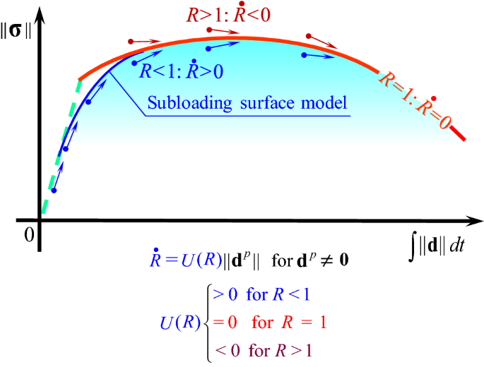

  

  Stress is automatically attracted to the normal-yield surface in subloading surface model

• (7) The outward-normal $\mathbf{n}$ at the peak stress point in the subloading surface is approximately coincides with the outward-normal of the plastic potential surface adopted in the Drucker–Prager model [9] as shown in Fig. 4 in which $\mathbf{n}^{\text{DP}}$ designates the outward-normal of the Drucker–Prager yield surface. Therefore, the associated flow rule can be adopted in the subloading surface model. On the other hand, the non-associated flow must be adopted in the Cap model composed of the Drucker–Prager model in the over-consolidated state and the Cam-clay model [61, 62] in the normal-consolidated state in order to suppress the excessive volumetric expansion in the over-consolidated state, which leads to the asymmetry of the elastoplastic tangent modulus tensor.

• (8) The exact finite strain elastoplastic constitutive equation, i.e., the multiplicative hyperelastic-based plastic constitutive equation can be formulated only by incorporating the subloading surface model (Hashiguchi [29, 32, 33], Hashiguchi and Yamakawa [42]).

  Fig. 4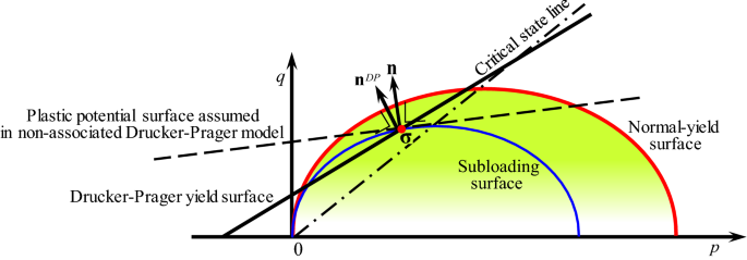

  

  Outward-normal of subloading surface, which coincides approximately with the plastic potential surface assumed in the Drucker–Prager model [9]

4 Material functions for granular materials

The material functions included in the subloading surface model described above are now formulated for a wide range of granular materials involving clays and sands, generalizing the past formulations to achieve the accurate description of cyclic loading behavior up to the cyclic mobility.

4.1 Elastic moduli

The elastic bulk modulus $K$ and the elastic shear modulus $G$ are given by Hashiguchi [31], modifying the former equations to describe the pressure-dependency (Hashiguchi [23, 32], Hashiguchi and Chen [34]) as follows:

$$K = \frac{-\dot{p}}{d_{\text{v}}^{\text{e}}} = \frac{p + \vartheta F}{\tilde{\kappa }}, \quad G = \frac{{\left\Vert {\mathop{\varvec{\upsigma}}\limits^{\circ}}{}^{\prime} \right\Vert}}{2 {\left\Vert {\mathbf{d}^{\text{e} \prime}} \right\Vert}} = G_{0} \left( \frac{p + \vartheta F}{p_{0} + \vartheta F_{0}} \right)^{n}$$

(48)

where $\tilde{\kappa}$ represents the slope of the swelling curve in the linear relation $\ln v - \ln p$ with both logarithms of volume $v$ and pressure $p$ in the isotropic consolidation. The term $\vartheta F$ is incorporated so that $K$ and $G$ are applicable even for the negative pressure range. Here, $\vartheta$ is a material constant leading to $\varepsilon_{\text{v}}^{\text{e}} \to \infty$ (infinite volume expansion) for $p \to - \vartheta F$, while $\vartheta \; (0 \le \vartheta < 0.1)$ for common clays and sands (Hashiguchi and Chen [34], Hashiguchi and Mase [35]). $d_{\text{v}}^{\text{e}}$ is the elastic volumetric strain rate $d_{\text{v}}^{\text{e}} \equiv \mathop{\mathrm{tr}} \mathbf{d}^{\text{e}}$. The power function of the pressure in Eq. (48) for the shear modulus is referred to Tatsuoka et al. [64]. $n \; (\le 1)$ is a material constant, while $n \cong 0.5$ is chosen for most sands. Consequently, the elastic tangent modulus depends naturally on pressure $p$ and isotropic hardening function $F$. The elastic moduli in Eq. (48) hold for granular materials consistently in the frameworks of the infinitesimal elasticity, the hypoelasticity and multiplicative hyperelasticity as was verified by Hashiguchi [31].

4.2 Yield and subloading functions

Let the normal-yield surface be given by the modified Cam-clay model (Burland [7], Roscoe and Burland [61]):

$$p \left[ 1 + \left( \frac{\| \varvec{\upsigma}{}^{\prime} \| / p}{M} \right)^{2} \right] = F$$

(49)

i.e.

$$\left( \frac{p - (1/2)F}{F/2} \right)^{2} + \left( \frac{\| \varvec{\upsigma}{}^{\prime} \|}{MF/2} \right)^{2} = 1$$

(50)

where $M$ is the stress ratio $\| \varvec{\upsigma}{}^{\prime} \| / p$ in the critical state. To take account of the influence of the third deviatoric stress invariant, $M$ is extended as follows (Hashiguchi [25]):

$$M = \frac{7}{8 + \cos 3 \theta_{\varvec{\upsigma}}} M_{\text{c}} = \frac{14\sqrt 6 \sin \phi_{\text{c}}}{(3 - \sin \phi_{\text{c}})(8 + \cos 3 \theta_{\varvec{\upsigma}})}$$

(51)

where $\theta_{\varvec{\upsigma}}$ is the so-called Lode angle defined by

$$\cos 3 \theta_{\varvec{\upsigma}} \equiv \sqrt{6} \mathop{\mathrm{tr}} (\varvec{\uprho}{}^{\prime})^{3}, \quad \varvec{\uprho}{}^{\prime} \equiv \frac{\varvec{\upsigma}{}^{\prime}}{\| \varvec{\upsigma}{}^{\prime } \|}$$

(52)

and

$$M_{\text{c}} \equiv \frac{2\sqrt{6} \sin \phi_{\text{c}} }{3 - \sin \phi_{\text{c}}}$$

(53)

$\phi_{\text{c}}$ being the angle of internal friction in the critical state for the axisymmetric, i.e., triaxial compression stress state $( \theta_{\varvec{\upsigma}} = \pi /3 \pm n(2\pi /3)) \; (n\colon \text{integer})$. The section of the normal-yield surface at the critical state given by Eq. (49) with Eq. (51) always fulfills the convexity condition as shown in Fig. 5 for the section of the critical state surface in the deviatoric stress plane. Equation (51) would be the simplest equation taking account of the third deviatoric stress invariant and fulfilling the convexity among various conical surface equations in the principal stress space [25].

Fig. 5

Section of the critical state surface in $\pi$-plane. (Coulomb–Mohr criterion is shown by dotted lines for reference)

Sands possess quite small strength in the negative pressure range. However, it is of crucial importance to shift the yield surface to the negative pressure range in order to describe rigorously the cyclic mobility, in which the stress changes actively around the null stress state. Here, it should be noticed that the shift of the yield surface is of the importance also in the computational aspect.

To shift the yield surface to the negative pressure range, Eq. (50) is modified by $\xi F$$(p \to p + \xi F)$ as follows (Hashiguchi and Mase [35]).

$$\left( \frac{p - ((1/2) - \xi )F}{F/2} \right)^{2} + \left( \frac{\| \varvec{\upsigma}{}^{\prime} \|}{MF/2} \right)^{2} = 1$$

(54)

where $\xi$ is the material constant, while it must fulfill $\xi \le 1/2$ since the tensile yield stress is smaller than the compression yield stress, and further the inequality $\xi < \vartheta$ is required since the volume does not become infinite by the elastic deformation inside the yield surface, satisfying $p \ge - \xi F > - \vartheta F$. The yield surface in Eq. (54) is shown in Fig. 6 in the pressure-deviatoric stress plane.

Fig. 6

Yield surface of granular materials with tensile strength

Equation (54) is extended by taking account of the rotation of the yield surface around the origin of the stress space into account and thus by replacing $\varvec{\upsigma}{}^{\prime}$ with $\varvec{\upsigma}{}^{\prime} - p \varvec{\upbeta}$, where $\varvec{\upbeta}$ is referred to as the rotational hardening variable represented by a deviatoric tensor, the evolution rule of which will be formulated in Sect. 4.4. This extension leads to

$$\left( \frac{p - ((1/2) - \xi )F}{F/2} \right)^{2} + \left( \frac{\left\Vert \overset{\frown}{\varvec{\upsigma}}{}^{\prime } \right\Vert}{\overset{\frown}{M} F/2} \right)^{2} = 1$$

(55)

where

$$\overset{\frown}{\varvec{\upsigma}}{}^{\prime} \equiv \varvec{\upsigma}^{\prime } - p \varvec{\upbeta}$$

(56)

$$\overset{\frown}{M} (\cos 3 \theta_{\overset{\frown}{\varvec{\upsigma}}})= \frac{14\sqrt{6} \sin \phi_{\text{c}}}{(3 - \sin \phi_{\text{c}}) (8 + \cos 3 \theta_{\overset{\frown}{\varvec{\upsigma}}} )} M_{\text{c}}$$

(57)

$$\cos 3\theta_{\overset{\frown}{\varvec{\upsigma}}} \equiv \sqrt{6} \mathop{\mathrm{tr}} ( \mathbf{t}_{\overset{\frown}{\varvec{\upsigma}}}^{\prime} )^{3}, \quad \mathbf{t}_{\overset{\frown}{\varvec{\upsigma}}}^{\prime} \equiv \frac{\overset{\frown}{\varvec{\upsigma}}{}^{\prime}}{{\left\Vert \overset{\frown}{\varvec{\upsigma}}{}^{\prime} \right\Vert}}$$

(58)

Equation (55) is rewritten as follows:

$$(1 - \xi ) \xi F^{2} + (1 - 2 \xi ) pF - (p^{2} + \overset{\frown}{\rho}{}^{2} ) = 0$$

(59)

where

$$\overset{\frown}{\rho } \equiv \frac{{\left\Vert \overset{\frown}{\varvec{\upsigma}}{}^{\prime} \right\Vert}}{\overset{\frown}{M}}$$

(60)

Equation (59) is the quadratic equation of the hardening function $F$. By solving this equation, it can be described in the separated form to the function $f ( p, \overset{\lower0.5em\hbox{$\smash{\scriptscriptstyle\frown}$}}{\rho} )$ and the hardening function $F$ as follows:

$$f ( p, \overset{\frown}{\rho} ) = F,\,f ( \varvec{\upsigma}, \varvec{\upbeta} ) = f ( p, \overset{\frown}{\rho} ) = \left\{\begin{array}{ll} p \bigl[ 1 + ( \overset{\frown}{\rho} / p )^{2} \bigr] & \text{for}\,\, \xi = 0 \\ \dfrac{1}{\tilde{\xi}} \bigl( \overset{\frown}{p}_{\rho } - \overline{\xi} p \bigr) & \text{for}\,\, \xi \ne 0 \end{array}\right.$$

(61)

where

$$\tilde{\xi} \equiv 2 ( 1 - \xi ) \xi, \quad \overline{\xi} \equiv 1 - 2 \xi, \quad \overset{\frown}{p}_{\rho} \equiv \sqrt{p^{2} + 2 \tilde{\xi} \overset{\frown}{\rho}{}^{2}}$$

(62)

Note that an analytically separated form cannot be derived from the yield conditions other than the modified Cam-clay model, e.g. the original Cam-clay model (Schofield and Wroth [62]) which is shifted to the negative pressure range by $p \to p + \xi F$ leading to $p \exp \bigl[ \| \varvec{\upsigma}{}^{\prime} \| / (pM) \bigr] = F \; \to \; (p + \xi F) \exp \bigl[ \| \varvec{\upsigma}{}^{\prime} \| / \{ (p + \xi F) M \} \bigr] = F$.

Further, let the subloading stress function $f ( \overline{\varvec{\upsigma}}, \varvec{\upbeta} )$ in Eq. (5) be given from Eq. (61) by replacing $\varvec{\upsigma}$ for the normal-yield surface to $\overline{\varvec{\upsigma}}$ for the subloading surface, i.e., $\overset{\frown}{\varvec{\upsigma}}{}^{\prime}$ to $\overset{\frown}{\overline{\varvec{\upsigma}}}{}^{\prime}$ as follows:

$$f ( \overline{\varvec{\upsigma}}, \varvec{\upbeta} ) = f ( \overline{p}, \overset{\frown}{\overline{\rho}} ) = \left\{\begin{array}{ll} \overline{p} \bigl[ 1 + \bigl( \overset{\frown}{\overline{\rho}} / \overline{p} \bigr)^{2} \bigr] & \text{for}\,\,\xi = 0 \\ \dfrac{1}{\tilde{\xi}} \bigl( \overset{\frown}{\overline{p}}_{\rho} - \overline{\xi } \overline{p} \bigr) & \text{for}\,\,\xi \ne 0 \end{array}\right.$$

(63)

where

$$\overset{\frown}{\overline{p}}_{\rho} \equiv \sqrt{ \overline{p}{}^{2} + 2\tilde{\xi } \overset{\frown}{\overline{\rho}}{}^{2} } \quad \bigl( \overline{p} \equiv - (\mathop{\mathrm{tr}} \overline{\varvec{\upsigma}} ) /3 \bigr)$$

(64)

$$\overset{\frown}{\overline{\rho}} \equiv \frac{{\left\Vert \overset{\frown}{\overline{\varvec{\upsigma}}}{}^{\prime} \right\Vert}}{\overset{\frown}{\overline{M}}}, \quad \overset{\frown}{\overline{\varvec{\upsigma}}}{}^{\prime} \equiv \overline{\varvec{\upsigma}}{}^{\prime} - \overline{p} \varvec{\upbeta}$$

(65)

$$\overset{\frown}{\overline{M}} ( \cos 3 \theta _{\overset{\frown}{\overline{\varvec{\upsigma}}}}) = \frac{14 \sqrt{6} \sin \phi_{\text{c}}}{( 3 - \sin \phi_{\text{c}} ) (8 + \cos 3 \theta _{\overset{\frown}{\overline{\varvec{\upsigma}}}} ) }$$

(66)

$$( \cos 3 \theta _{\overset{\frown}{\overline{\varvec{\upsigma}}}}) \equiv \sqrt{6} \mathop{\mathrm{tr}} ( \overset{\frown}{\overline{\varvec{\uprho}}}{}^{\prime} )^{3}, \quad \overset{\frown}{\overline{\varvec{\uprho}}}{}^{\prime} \equiv \frac{\overset{\frown}{\varvec{\overline{\upsigma}}}{}^{\prime} }{{\left\Vert \overset{\frown}{\varvec{\overline{\upsigma}}}{}^{\prime} \right\Vert}}$$

(67)

4.3 Isotropic hardening by volumetric and deviatoric plastic strain rates

The hardening function in Eqs. (4) or (5) is given as follows (Hashiguchi [32]):

$$F(H) = F_{0} \exp \left( \frac{H}{\tilde{\lambda} - \tilde{\kappa}} \right), \quad F^{\prime} \equiv \frac{dF}{dH} = \frac{1}{\tilde{\lambda} - \tilde{\kappa}} F$$

(68)

where $\tilde{\lambda }$ and $\tilde{\kappa }$ stand for the slopes of the normal-consolidation curve and the swelling curve, respectively, in the $\ln v - \ln (p + \vartheta F)$ plane (Hashiguchi [23]), which is based on the following isotropic consolidation characteristics.

$$\left\{ \begin{array}{ll} \varepsilon_{\text{v}}^{\text{e}} = \ln \dfrac{v}{\overline{v}} = - \tilde{\kappa} \ln \dfrac{p + \vartheta p_{\text{y}}}{p_{0} + \vartheta p_{\text{y0}}} \\ \varepsilon_{\text{v}}^{\text{p}} = \ln \dfrac{\overline{v}}{v_{0}} = - (\tilde{\lambda} - \tilde{\kappa}) \ln \dfrac{p_{\text{y}}}{p_{\text{y0}}} \end{array} \right.$$

(69)

where $\varepsilon_{\text{v}}^{\text{e}}$ and $\varepsilon_{\text{v}}^{\text{p}}$ are the elastic and the plastic logarithmic volumetric strains, respectively; $v$, $v_{0}$ and $\overline{v}$ are the current volume, the initial volume and the volume unloaded state to the initial pressure, respectively; and $p$, $p_{0}$, $p_{\text{y}}$ and $p_{\text{y0}}$ are the current, the initial and the current yield and the initial yield pressure, respectively, as shown in Fig. 6. Replacing the pressures $p_{\text{y}}$ and $p_{\text{y0}}$ to the isotropic hardening function $F$ and its initial value $F_{0}$, respectively, in Eq. (69), one has

$$\left\{ \begin{array}{ll} \varepsilon_{\text{v}}^{\text{e}} = - \tilde{\kappa} \ln \dfrac{p + \vartheta F}{p_{0} + \vartheta F_{0}} \\ \varepsilon_{\text{v}}^{\text{p}} = - (\tilde{\lambda } - \tilde{\kappa}) \ln \dfrac{F}{F_{0}} \end{array} \right.$$

(70)

The isotropic hardening function is given from Eq. (70) by choosing the isotropic hardening variable $H$ to be the plastic volumetric contraction, i.e., $H = - \varepsilon_{\text{v}}^{\text{p}}$ as follows:

$$F(H) = F_{0} \exp \left( \frac{H}{\tilde{\lambda} - \tilde{\kappa}} \right)$$

(71)

The rate of isotropic hardening/softening variable $H$ was extended by Nova [57] and Wilde [67] to incorporate the influence of the deviatoric plastic strain rate, called the deviatoric (isotropic) hardening, in addition to the volumetric plastic strain rate described above. Here, aiming at establishing a quantitative description of cyclic mobility, let $\dot{H}$ be extended to depend on the plastic volumetric strain rate $d_{\text{v}}^{\text{p}}$ and the plastic shear rate $d_{\text{s}}^{\text{p}}$ for a wide range of stress up to the negative pressure as follows (Fig. 6):

$$\dot{H} = -d_{\text{v}}^{\text{p}} + d_{\text{s}}^{\text{p}} = \dot{\bar{\lambda}} h$$

(72)

$$d_{\text{v}}^{\text{p}} \equiv \mathop{\mathrm{tr}} \mathbf{d}^{\text{p}}, \quad \mathbf{d}^{\text{p}\prime} \equiv \mathbf{d}^{\text{p}} - (d_{\text{v}}^{\text{p}}/3)\,\mathbf{I}$$

(73)

$$\begin{aligned} & d_{\text{s}}^{\text{p}} = \mu _{\text{d}} \| \mathbf{d}^{\text{p}\prime} \| \frac{\chi_{\text{d}}^{a} - 1}{\chi _{\text{d}}^{a} - 1 + b} \\ & \quad \left\{\begin{array}{ll} > 0 & \text{(deviatoric hardening) for} \, \chi_{\text{d}} > 1 \\ = 0 & \text{(deviatoric non-hardening) for}\,\, \chi_{\text{d}} = 1 \\ < 0 & \text{(deviatoric softening) for}\,\, \chi_{\text{d}} < 1 \end{array}\right. \end{aligned}$$

(74)

$$\chi_{\text{d}} \equiv \frac{\| \varvec{\upsigma}{}^{\prime} \| / (p + \vartheta F)}{M_{\text{d}}}$$

(75)

$$M_{\text{d}} (\cos 3 \theta_{\varvec{\upsigma}} ) \equiv \frac{14 \sqrt{6} \sin \phi_{\text{d}}}{(3 - \sin \phi_{\text{d}}) (8 + \cos 3 \theta_{\varvec{\upsigma}} )}$$

(76)

$$h = - \mathop{\mathrm{tr}} \overline{\mathbf{n}} + \mu_{\text{d}} \| \overline{\mathbf{n}}{}^{\prime} \| \, \frac{\chi_{\text{d}}^{a} - 1}{\chi_{\text{d}}^{a} - 1 + b}$$

(77)

where $\mu_{\text{d}}$, $\phi_{\text{d}} \; ( < \phi_{\text{c}} )$, $a \; ( \ge 1)$ and $b \; ( > 1)$ are material constants. Here, $\phi_{\text{d}} < \phi_{\text{c}}$ holds in general since the deviatoric stress can increase over the critical state ($\mathop{\mathrm{tr}} \overline{\mathbf{n}} = 0 \; \leadsto \; \mathop{\mathrm{tr}} \mathbf{d}^{\text{p}} = 0$) when the stress ratio increases at a low pressure under the undrained condition even in loose sands. $M_{\text{d}}$ in Eq. (76) is formulated analogously to $M$ in Eq. (51). Hardening and softening are induced outside and inside, respectively, the conical surface $\| \varvec{\upsigma}{}^{\prime} \| = M_{\text{d}} (p + \vartheta F)$ which is called the deviatoric hardening boundary surface. It is extended to accommodate the negative pressure $p \; ( -\vartheta F < p \le 0)$ by replacing the normalized stress ratio $(\| \varvec{\upsigma}{}^{\prime} \| / p) / M_{\text{d}}$ to $\chi_{\text{d}}$ defined in Eq. (75). The deviatoric hardening rate depends nonlinearly on the modified stress ratio $\chi_{\text{d}}$ with the upper limit $\mu_{\text{d}} \| \mathbf{d}^{p \prime} \|$ of the plastic shear rate $d_{\text{s}}^{\text{p}}$ (Fig. 7).

Fig. 7

Deviatoric hardening/softening

4.4 Rotational hardening: Anisotropic hardening by rotation of yield surface

The rotational hardening rule is formulated by

• (1) postulating that the central axis $\varvec{\upsigma}{}^{\prime } / p = \varvec{\upbeta}$ of the normal-yield surface rotates towards the conjugate generating line $\varvec{\upsigma}{}^{\prime} /p = \overset{\frown}{\overline{M}}_{\text{r}} \, \overset{\frown}{\overline{\varvec{\uprho}}}{}^{\prime}$ on the rotational limit surface $\| \varvec{\upsigma}{}^{\prime} \| / p = \overset{\frown}{\overline{M}}_{\text{r}}$,

• (2) noting that the anisotropic hardening is induced only by the deviatoric plastic strain rate as follows (Fig. 8):

  $$\mathop{\varvec{\upbeta}}\limits^{\circ} = b_{\text{r}} \left( \mathbf{d}^{\text{p} \prime} - \frac{1}{\overset{\frown}{\overline{M}_{\text{r}}} }\Vert \mathbf{d}^{\text{p} \prime } \Vert \, \varvec{\upbeta} \right) = \mathbf{b} \dot{\bar{\lambda}}$$

  (78)

where

$$\overset{\frown}{\overline{M}} \left( \cos 3 \theta _{\overset{\frown}{\overline{\varvec{\upsigma}}}} \right) = \frac{14 \sqrt{6} \sin \phi_{\text{r}}}{( 3 - \sin \phi_{\text{r}} ) (8 + \cos 3 \theta _{\overset{\frown}{\overline{\varvec{\upsigma}}}} ) }$$

(79)

$$\overset{\frown}{\overline{\varvec{\upsigma}}}{}^{\prime } \equiv \overline{\varvec{\upsigma }}{}^{\prime } - \overline{p} \varvec{\upbeta}, \,\,\mathbf{t}_{\overset{\frown}{\overline{\varvec{\upsigma}}}}^{\prime} \equiv \frac{\overset{\frown}{\overline{\varvec{\upsigma}}}{}^{\prime}} {\left\Vert \overset{\frown}{\overline{\varvec{\upsigma}}}{}^{\prime} \right\Vert},\,\, \cos 3 \theta_{\overset{\frown}{\overline{\varvec{\upsigma}}}} \equiv \sqrt{6} \mathop{\mathrm{tr}} \left({\mathbf{t}_{\overset{\frown}{\overline{\varvec{\upsigma}}}}^{\prime}}\right) ^{3}$$

(80)

$$\mathbf{b} = b_{\text{r}} \left( \overline{\mathbf{n}}{}^{\prime } - \frac{1}{\overset{\frown}{\overline{M}}_{\text{r}}} \Vert \overline{\mathbf{n}}{}^{\prime } \Vert \, \varvec{\upbeta} \right)$$

(81)

Fig. 8

Yield surface and rotational limit surfaces illustrated in the principal stress space

$b_{\text{r}}$ is the material constant regulating the rate of the rotation. $\overset{\frown}{\overline{M}}_{\text{r}}$ is formulated analogously to $M$ in Eqs. (51), (57) and (76), where $\phi_{\text{r}}$ is the material constant denoting the limit of the rotational angle of the normal-yield and subloading surfaces. Note here that Eq. (78) takes a form analogous to the evolution equation of back stress tensor in the nonlinear kinematic hardening rule [5]. For the subloading surface in Eq. (63) based on the modified Cam-clay model, the rotation does not occur, i.e., $\mathop{\varvec{\upbeta}}\limits^{\circ} = \mathbf{0}$ when the stress lies on the central axis of the subloading surface, fulfilling $\overline{\varvec{\upsigma}}{}^{\prime} = \overline{p} \varvec{\upbeta}$, for which $\overline{\mathbf{n}}{}^{\prime} = \mathbf{0}$ leading to $\mathbf{d}^{\text{p} \prime} = \mathbf{0}$ holds as shown in Fig. 1.

4.5 Extension of material parameter for evolution of normal-yield ratio

The material parameter $\overline{u}$ in the evolution equation (41) of the normal-yield ratio is extended as follows (Fig. 9):

$$\overline{u} = \frac{u_{0}}{\overset{\frown}{\overline{M}}{}^{\overline{m}} \exp \bigl( u_{\varepsilon} \varepsilon^{\text{p} \prime} \bigr)}$$

(82)

where

$$\varepsilon^{\text{p} \prime} \equiv \int_{0}^{t} \| \mathbf{d}^{\text{p} \prime} \| \, dt$$

(83)

Fig. 9

Extension of material parameter $\overline{u}$

$u_{0}$, $\overline{m}$ and $u_{\varepsilon }$ are material constants. The material parameter $\overline{u}$ becomes smaller inducing a larger plastic strain rate as the accumulation of the deviatoric plastic strain rate proceeds, while this trend is more notable for larger values of $u_{\varepsilon}$. In addition, $\overline{u}$ is inversely proportional to $\overset{\frown}{\overline{M}}$ and therefore a larger plastic strain rate is induced in the compression side than in the tension side, while this trend is more notable for larger value of $\overline{m}$.

5 Summary of material parameters and their physical meanings

Not a few material parameters, i.e., nineteen material constants and three initial values of internal variables are incorporated in the present elastoplastic constitutive equation in order to describe the cyclic mobility accurately. They are shown collectively in the following.

Material constants:

• Elastic moduli $\tilde{\kappa}, \; G_{0}, \; n$

• Yield surface (ellipsoid)$\phi_{\text{c}}, \; \xi \; (< 0.5)$

• Isotropic hardening/softening $\left\{\begin{array}{ll} \text{volumetric: } \tilde{\lambda}, \; \vartheta \; (> \xi) \\ \text{deviatoric: } \mu_{\text{d}}, \; \phi_{\text{d}} \; (< \phi_{\text{c}}), \; a \; (\ge 1), \; b \; (\ge 1), \end{array}\right.$

• Anisotropic (rotational) $\text{hardening: } b_{\text{r}}, \; \phi_{\text{r}}$

• Normal - yield ratio $u_{c}, \; \overline{u}, \; u_{\varepsilon}, \; \overline{m}$

• Similarity - center $\text{: } c_{\text{e}}, \; \chi \; (< 1)$

Initial values of internal variables:

• Isotropic hardening function $F_{{0}}$.

• Rotational hardening $\varvec{\upbeta}_{0}$.

• Elastic-core $\mathbf{c}_{0}$.

$F_{0}$, $G_{{0}}$, $\vartheta$, $\phi_{\text{c}}$, $\xi$, $\overline{u}$, $c_{\text{e}}$ and $\chi$ are larger but $\phi_{\text{d}}$, $\tilde{\lambda}$ and $\tilde{\kappa}$ are smaller in denser granular materials with higher strength for same arrangement of particles.

The main influences of the material constants on the deformation behavior are described below.

• 1. The transition from the elastic to plastic state is gentler for smaller $u_{0}$ values.

• 2. Axial strain is induced more intensely in the triaxial compression side for larger $\overline{m}$ values.

• 3. Strain rate increases more rapidly with the accumulated deviatoric plastic strain for larger $u_{\varepsilon}$ values.

• 4. The difference between the tangent stiffness moduli in reloading and reverse loading is larger and thus the difference between the curvatures of the stress–strain curves in them is larger for larger $u_{\text{c}}$ values.

• 5. Plastic deformation begins sooner after unloading for larger $c_{\text{e}}$ values for which the closed hysteresis loop is depicted so that the strain accumulation is suppressed. On the other hand, the open hysteresis loop is depicted for $c_{\text{e}} = 0$, returning to the initial subloading surface model.

• 6. The material constant $\phi_{\text{d}}$, which regulates the boundary of the deviatoric hardening and softening, is larger for a looser material with a wider range of deviatoric softening.

• 7. The normal-yield and subloading surfaces rotates in a wider range for a larger $\phi_{\text{r}}$ value. They rotate more rapidly with the deviatoric plastic strain for larger value of $b_{\text{r}}$.

The identifications of the material parameters are commented below.

$\tilde{\lambda }$ and $\tilde{\kappa }$ are determined by the curve-fitting to the test data of the isotropic consolidation. Also, they can be known easily by $\tilde{\lambda} = \lambda /(1 + e_{0}), \; \tilde{\kappa} = \kappa /(1 + e_{0})$, if there is past data of $\lambda$ and $\kappa$ in the $e - \log p$ linear relation.

$G_{0}$ and $n$ are determined from the stress vs. strain curve under constant pressure inside the yield surface, while we may use $n = 0.5$ usually.

$\phi_{\text{c}}$ is determined by the inclination of the critical state line in the triaxial compression.

$\xi$ is determined from the pressures in the isotropic compression and the extension test.

$\mu_{\text{d}}, \; \phi_{\text{d}}, \; a, \text{and } b$ are determined from the undrained triaxial compression test data.

$b_{\text{r}}$ and $\phi_{\text{r}}$ are determined from the loading and unloading process in the triaxial compression or extension test.

$u_{c}, \; \overline{u}, \; u_{\varepsilon},\text{ and } \overline{m}$ are inferred from the reloading curve in the drained test.

$c_{\text{e}}$ and $\chi$ are determined from the loading–unloading curve, while we may put $\chi = 0.7$ usually.

$F_{{0}}$ can be determined from the initial normal-consolidation stress.

$\varvec{\upbeta}_{0}$ may be chosen to be $\varvec{\upbeta}_{0} = \mathbf{0}$ in isotropic-consolidated sands but it can be calculated from $K_{0}$-value in a $K_{0}$-consolidation.

${\mathbf{c}}_{{0}}$ is determined from the stress at which the most elastic behavior is observed.

6 Simulations of test data for cyclic mobility

The constitutive equation of granular materials formulated in the previous sections is applied to the simulations of various test data on the cyclic mobility under the undrained condition with the constant deviatoric stress amplitudes.

All the test data adopted for the simulations were obtained by the cyclic triaxial compression/extension tests with symmetric constant deviatoric stress amplitudes from the isotropic stress state under constant total lateral confining pressures denoted by $p_{\text{c}}$. The initial isotropy, i.e., $\varvec{\upbeta}_{0} = \mathbf{0}$ is assumed and the typical values $n = 0.5$ and $\chi = 0.7$ are used for all test data. Further, the substructure spin is set to be zero because of the triaxial test in which the rotation of material is not induced so that the corotational-time derivative coincides with the material-time derivative. The physical properties of the tested sands, the test condition and the material parameters used in the simulations are listed in Table 1.

Table 1 Physical properties of tested sands, test condition and material parameters in simulations

The simulation results of the Toyoura sand with the almost same initial void ratio $(e_{0} = 0.722{\text{ and }}0.718)$ are shown for Figs. 10 and 11, while the same values of the material parameters are used in these simulations. Further, the simulations of the Tone river sand and the Edo river sand are shown for Figs. 12 and 13, respectively. The butterfly-shaped stress paths after the gradual decreases of the pressure and the deviatoric stress vs. axial strain curves with the increasing amplitudes of axial strain are simulated in these figures. The test results are simulated well in these calculations, where various stress ratios and numbers of loading cycles are applied. The maximum amplitudes of the axial strain are simulated well even for the high loading cycles up to the eighty-seven cycles. However, the deceases of the pressure are more gradual in the simulations than in the test results. The amplitudes of the axial strain in the simulations are smaller at the beginnings and later become larger compared with the test results in Figs. 10 and 11 for the Toyoura sand. The stress paths in the simulations are warped inversely to the test results in Figs. 12 and 13 for the Tone river sand and the Edo river sand. Further improvements would be required for a more accurate prediction of cyclic mobility.

Fig. 10

Simulation of test data for Toyoura sand after Yamada and Noda [68] ($e_{0}$ = 0.722, $D_{r}$ = 76%, $p_{\text{c}}$ = 100 kPa, stress ratio amplitude = $\pm$ 0.39, cyclic number = 9)

Fig. 11

Simulation of test data for Toyoura sand after Yamada and Noda [68] ($e_{0}$ = 0.718, $D_{r}$ = 77%, $p_{\text{c}}$ = 100 kPa, stress ratio amplitude = $\pm$ 0.44, cyclic number = 7)

Fig. 12

Simulation of test data for Tone river sand after Kiyota et al  [48, 49]. ($e_{0}$ = 0.739, $D_{r}$ = 84%, $p_{\text{c}}$ = 100 kPa, stress ratio amplitude = $\pm$ 0.80, cyclic number = 87)

Fig. 13

Simulation of test data for Edo river sand after Kiyota et al  [48, 49]. ($e_{0}$ = 0.762, $D_{r}$ = 88%, $p_{\text{c}}$ = 160 kPa, stress ratio amplitude = $\pm$ 0.60, cyclic number = 20)

Since seismic waves cause the cyclic loading at high frequency, the ground deformation occurs under fully or nearly undrained condition during an earthquake. However, when the earthquake ceases, the vertical load due to the weight of the ground and the gravity of the building floating during the earthquake acts to the soil grounds pushing out the pore water, and thus the soil skeleton deforms under the drained conditions. Therefore, it is required to describe both the cyclic mobility under undrained condition and the monotonic loading behavior under drained condition by a unique elastoplastic constitutive equation with a unified set of material parameters. On the other hand, although there are few test results of cyclic mobility and drained tests on specimens of the same material and the same void ratio, the results of drained tests obtained using Toyoura used in the above-mentioned cyclic mobility are provided from the same experimenter to the authors [69]. The simulation result under the drained condition is shown in Fig. 14, where the tested and the calculated stress and volume strain curves are shown. Therein, since the initial void ratio $e_{0} = 0.748$ in the drained test is sufficiently close to $e_{0} = 0.722$ and 0.718 in the above-mentioned cyclic mobility test, the material parameters shown in Table 1 (which are used in Figs. 10 and 11) are used. A fairly good simulation to the test result is seen in this figure.

Fig. 14

Simulation of test data for Toyoura sand in drained condition after Yamada [69] ($e_{0}$ = 0.748, $D_{r}$ = 69%, $p_{\text{c}}$ = 98.1 kPa)

Incidentally, for reference, the simulation to the drained test result with the initial void ratio $e_{0} = 0.924$ (looser than in Fig. 14) of the Toyoura sand is shown in Fig. 15, choosing the material parameters as follows:

$$\tilde{\lambda} = 0.02, \, \tilde{\kappa } = 0.0007, \, G_{0} = 100\,{\text{MPa}}, \, \vartheta = 0.1, \, \phi_{\text{c}} = 30^{ \circ} ,$$

$$\xi = 0.005, \, \mu_{\text{d}} = 1, \, \phi_{\text{d}} = 18^{ \circ }, \, a = 1, \, b = 6, b_{\text{r}} = 1, \, \phi_{\text{r}} = 5^{ \circ},$$

$$u_{\text{c}} = 3, \, \overline{u} = 10, \, u_{\varepsilon} = 9, \, \overline{m} = 10, \, c_{\text{e}} = 5,$$

$$F_{0} = 170\,{\text{kPa}}, \, {\mathbf{c}}_{0} = -60\,{\mathbf{I}}$$

Fig. 15

Simulation of test data for Toyoura sand in drained condition after Yamada [69] ($e_{0}$ = 0.924, $D_{r}$ = 18%, $p_{\text{c}}$ = 98.1 kPa)

7 Conclusion

In this article, the subloading surface model is elaborated to describe the cyclic mobility observed prior to the liquefaction induced by earthquakes. The results obtained in this study are summarized as follows:

• 1. The elastoplastic constitutive equation of geomaterials is elaborated by the formulations of

• 2. the rigorous evolution rule of the elastic-core, which is of crucial importance for the description of cyclic loading behavior,

• 3. the evolution rule of the rotational hardening, which is of crucial importance for the description of the anisotropic hardening behavior of granular materials,

• 4. the material functions for the elastic moduli extended to the pressure dependence, the yield condition extended to the negative pressure range, the isotropic hardening rule based on not only the volumetric but also the deviatoric plastic deformations for the accurate description of the cyclic loading behavior up to the cyclic mobility.

• 5. Then, the validity of the proposed constitutive equation based on the subloading surface model for granular materials was verified by the comparisons with the test data on the cyclic mobility in three kinds of sands for various numbers of cycles under various stress amplitudes. The butterfly-shaped stress path in the pressure vs. deviatoric stress plane and the S-shaped deviatoric stress vs. axial strain loops were reproduced accurately.

• 6. The present formulation would provide the substantial foundation for the elastoplastic description of cyclic mobility, although further elaboration is desirable for a highly accurate description of the cyclic mobility.

• 7. The present constitutive model would be applicable to the predictions of the deformation behavior not only during the earthquake but also after it.

Not a few material constants are incorporated in order to describe the cyclic mobility accurately by the elastoplastic constitutive equation because it is to be one of the most complicated mechanical phenomena in the natural world. Further study is required to clarify their definite physical meanings for formulating a more sophisticated constitutive equation of geomaterials.

The formulation falls within framework of the hypoelastic-based plasticity which is limited to the description of the infinitesimal elastic deformation and requires the cumbersome time-integrations of corotational rates of stress and internal variables. Then, it should be extended to the multiplicative hyperelastic-based plasticity (Hashiguchi [29, 33], Hashiguchi and Yamakawa [42]) with a rigorous description of hyperelastic equation of granular materials (Hashiguchi [31]) for further accurate description of cyclic mobility up to the finite deformation.

References

Akiyoshi T, Matsumoto H, Fuchida K, Fang HL (1994) Cyclic mobility behaviour of sand by the three-dimensional strain space multimechanism model. Int J Numer Anal Methods Geomech 18:397–415
Anjiki T, Oka M, Hashiguchi K (2016) Elastoplastic analysis by complete implicit stress-update algorithm based on the extended subloading surface model. Trans Jpn Soc Mech Eng. https://doi.org/10.1299/transjsme.16-00029 ((in Japanese))
Anjiki T, Oka M, Hashiguchi K (2019) Elastoplastic analysis by return-mapping method with rigorous loading criterion for extended subloading surface model. Trans Jpn Soc Mech Eng. https://doi.org/10.1299/transjsme.18-00327 ((in Japanese))
Anjiki T, Oka M, Hashiguchi K (2019) Complete implicit stress integration algorithm with extended subloading surface model for elastoplastic deformation analysis. Int J Numer Methods Eng 121:945–966
Armstrong PJ, Frederick CO (1966) A mathematical representation of the multiaxial Bauschinger effect. Report RD/B/N 731 (or Mater. High Temp. 24, 1–6, 2007).
ASCE (1978) The committee on soil dynamics of the geotechnical engineering division: Definition of terms related to liquefaction. J Geotech Eng Div ASCE 104(9):1197–1200
Burland JB (1965) The yielding and dilatation of clay. Corresp Géotech 15:211–214
Desai CS, Park I, Shao C (1998) Fundamental yet simplified model for liquefaction instability. Int J Numer Anal Methods Geomech 22:721–748
Drucker DC, Prager W (1952) Soil mechanics and plastic analysis for limit design. Quart Appl Math 10:157–165
Elgamal A, Yang Z, Parra E, Ragheb A (2003) Modeling of cyclic mobility in saturated cohesionless soils. Int J Plast 19:883–905
Fang HL, Zheng H, Zheng J (2017) Micromechanics-based multi mechanism bounding surface model for sands. Int J Plast 90:242–266
Fincato R, Tsutsumi S (2018) A return mapping algorithm for elastoplastic and ductile damage constitutive equations using the subloading surface method. Int J Numer Methods Eng 113:1729–1754. https://doi.org/10.1002/nme.5718
Fu Y, Iwata M, Ding W, Zhang F, Yashima A (2012) An elastoplastic model for soft sedimentary rock considering inherent anisotropy and confining-stress dependency. Soils Found 52:575–589
Fuente MDL, Vaunat J, Marin-Moreno H (2019) A densification mechanism to model the mechanical effect of methane hydrates in sandy sediments. Int J Numer Anal Methods Geomech 27:1–21
Gang W, Horikoshi K, Akiyoshi A (2020) Effects of internal erosion on parameters of subloading Cam-Clay model. Geotech Geol Eng 38:1323–1335
Ghasemzadeh H, Ghoreishian Amiri SA (2013) A hydro-mechanical elastoplastic model for unsaturated soils under isotropic loading conditions. Comput Geotech 51:91–100
Gerolymos N, Gazetas G (2005) Constitutive model for 1-D cyclic soil behaviour applied to seismic analysis of layered deposits. Soils Found 45(3):147–159
Hashiguchi K. (1975) Plastic constitutive equation of soils with hardening/softening behavior. Dr. Thesis (Engineering), Tokyo Institute of Technology, Tokyo, pp. 1–365.
Hashiguchi K (1980) Constitutive equations of elastoplastic materials with elastic–plastic transition. J Appl Mech (ASME) 47:266–272
Hashiguchi K (1989) Subloading surface model in unconventional plasticity. Int J Solids Struct 25:917–945
Hashiguchi K (1993) Fundamental requirements and formulation of elastoplastic constitutive equations with tangential plasticity. Int J Plast 9:525–549
Hashiguchi K (1993) Mechanical requirements and structures of cyclic plasticity models. Int J Plast 9:721–748
Hashiguchi K (1995) On the linear relations of V–ln p and ln v–ln p for isotropic consolidation of soils. Int J Numer Anal Methods Geomech 19:367–376
Hashiguchi K (1997) The extended flow rule in plasticity. Int J Plast 13:37–58
Hashiguchi K (2002) A proposal of the simplest convex-conical surface for soils. Soils Found 42(3):107–113
Hashiguchi, K. (2009) Elastoplasticity Theory, First edition, Lecture Note in Appl. Compt. Mech., Springer–Verlag.
Hashiguchi K (2013) General description of elastoplastic deformation/sliding phenomena of solids in high accuracy and numerical efficiency: Subloading surface concept. Arch Compt Methods Eng 20:361–417
Hashiguchi K (2013) Elastoplasticity Theory. Second edition Lecture Note in Appl. Compt. Mech. Springer–Verlag
Hashiguchi K (2016) Exact formulation of subloading surface model: Unified constitutive law for irreversible mechanical phenomena in solids. Arch Comput Methods Eng 23:417–447
Hashiguchi K (2017) Foundations of Elastoplasticity: Subloading Surface Model. Springer-Verlag
Hashiguchi K (2018) Hypo- and hyper-elastic equations of soils. Int J Numer Anal Methods Geomech 42:1554–1564
Hashiguchi K (2019) Multiplicative hyperelatic-based plasticity for finite elastoplastic deformation/sliding: A comprehensive review. Arch Compt Methods Eng 26:597–637
Hashiguchi K (2020) Nonlinear Continuum Mechanics for Finite Elasticity-plasticity: Multiplicative Decomposition with Subloading Surface Model. Elsevier
Hashiguchi K, Chen Z-P (1998) Elastoplastic constitutive equations of soils with the subloading surface and the rotational hardening. Int J Numer Anal Methods Geomech 22:197–227
Hashiguchi K, Mase T (2007) Extended yield condition of soils with tensile strength and rotational hardening. Int J Plast 23:1939–1956
Hashiguchi K, Ozaki S (2008) Constitutive equation for friction with transition from static to kinetic friction and recovery of static friction. Int J Plast 24:2102–2124
Hashiguchi K, Ozaki S, Okayasu T (2005) Unconventional friction theory based on the subloading surface concept. Int J Solids Struct 42:1705–1727
Hashiguchi K, Saitoh K, Okayasu T, Tsutsumi S (2002) Evaluation of typical conventional and unconventional plasticity models for prediction of softening behavior of soils. Géotechnique 52:561–573
Hashiguchi K, Ueno M (2017) Elastoplastic constitutive equation of metals under cyclic loading. Int J Eng Sci 111:86–112
Hashiguchi K, Ueno M, Kuwayama T, Suzuki N, Yonemura S, Yoshikawa N (2016) Constitutive equation of friction based on the subloading-surface concept. Proc Royal Soc London A472:20160212. https://doi.org/10.1098/rspa.2016.0212
Hashiguchi K, Ueno M, Ozaki T (2012) Elastoplastic model of metals with smooth elastic-plastic transition. Acta Mech 223:985–1013
Hashiguchi K, Yamakawa Y. (2012) Introduction to Finite Strain Theory for Continuum Elasto-Plasticity. Wiley Series in Computational Mechanics, John Wiley.
Hashiguchi K, Yoshimaru T (1995) A generalized formulation of the concept of nonhardening region. Int J Plasticity 11:347–365
Iai S, Matsunaga Y, Kameoka T (1992) Strain space plasticity model for cyclic mobility. Soils Found 32(2):1–15
Iguchi T, Yamakawa Y, Ikeda K (2016) A re-formulation of extended subloading surface model for cyclic plasticity within small strain framework: hyperelastic-based formulation and fully implicit return-mapping scheme. Trans Jpn Soc Mech Eng 82(841):16–00197. https://doi.org/10.1299/transjsme.16-00197 ((in Japanese))
Iguchi T, Yamakawa K, Hashiguchi K, Ikeda K (2017) Extended subloading surface model based on multiplicative finite strain elastoplasticity framework: constitutive formulation and fully implicit return-mapping scheme. Trans Jpn Soc Mech Eng 83:1–20. https://doi.org/10.1299/transjsme.17-00008 ((in Japanese))
Iguchi T, Fukuda T, Yamakawa Y, Ikeda K, Hashiguchi K (2017) An improvement of loading criterion for stress calculation based on elastic predictor and return-mapping scheme for extended subloading surface plasticity model. J Appl Mech (JSCE) 20:363–375 ((in Japanese))
Kiyota T, Kozeki J, Sato T, Kuwano S (2009) Aging effects on small strain shear moduli and liquefaction properties of in-situ frozen and reconstituted sandy soils. Soils Found 49:259–274
Kiyota T, Kozeki J, Sato T, Tsutsumi Y (2009) Effects of sample disturbance on small strain characteristics and liquefaction properties of Holocene and pleistocene sandy soils. Soils Found 49(4):509–523
Masing, G. (1926) Eigenspannungen und Verfestigung beim Messing. Proc 2nd Int Congr Appl Mech, Zurich 332–335.
Mroz Z, Norris VA, Zienkiewicz OC (1981) An anisotropic critical state model for soils subject to cyclic loading. Géotechnique 31:451–469
MSC Software Corporation (2017) User manual for Hashiguchi model, Marc and Mentat Release Guide 2017.1, Material Behavior.
Nakai T, Hinokio M (2004) A simple elastoplastic model for normally and over consolidated soils with unified material parameters. Soils Found 44(2):53–70
Nakai T, Farias MM, Bastos D, Sato Y (2007) Simulation of conventional and inverted braced excavations using subloading model. Soils Found 47(3):597–612
Nakai T, Shahin HM, Kikumoto M, Kyokawa H, Zhang F, Farias MM (2011) A simple and unified three-dimensional model to describe various characteristics of soils. Soils Found 51(6):1149–1168
Noda T, Xu B, Asaoka A (2013) Acceleration generation due to strain localization of saturated clay specimen based on dynamic soil–water coupled finite deformation analysis. Soils Found 53(5):653–670
Nova R (1977) On the hardening of soils. Arch Mech Stos 29:445–458
Pedroso DM (2014) The subloading isotropic plasticity as a variable modulus model. Comput Geotech 61:230–240
Prevost JH, Keane CM (1994) Multimechanism elasto-plastic model for soils. J Eng Mech Div 116(9):1924–1944
Oka F, Yashima A, Tateishi Y, Taguchi Y, Yamashita A (1999) A cyclic elasto-plastic constitutive model for sand considering a plastic-strain dependence of the shear modulus. Géotechnique 49:661–680
Roscoe KH, Burland JB (1968) On the generalized stress-strain behaviour of ‘wet’ clay. Engineering Plasticity, Cambridge Univ. Press, pp. 535–608.
Schofield AN, Wroth CP (1968) Critical State Soil Mechanics. McGraw-Hill, London
Sekiguchi H, Ohta H. (1977) Induced anisotropy and its time dependence in clays, Constitutive Equations of Soils. Proc. Spec. Session 9, 9th Int. Conf. Soil Mech. Found. Eng., 229–238.
Tatsuoka F, Iwasaki T, Takagi Y (1978) Hysteretic damping of sands under cyclic loading and its relation to shear modulus. Soils Found 18(2):25–40
Truesdell C (1955) Hypo-elasticity. J Rational Mech Anal 4:83–133
Wongsaroj J, Soga K, Mair RJ (2007) Modeling of long-term ground response to tunneling under St James’ Park London. Géotechnique 57:75–90
Wilde P (1977) Two invariants depending models of granular media. Arch Mech Stos 29:799–809
Yamada S, Noda T. (2018) The test data provided to the authors by the private communication.
Yamada S (2021) The test data provided to the authors by the private communication.
Yamakawa Y, Hashiguchi K, Ikeda K (2010) Implicit stress-update algorithm for isotropic Cam-clay model based on the subloading surface concept at finite strains. Int J Plast 26:634–658
Yuanming L, Long J, Xiaoxiao C (2009) Yield criterion and elasto-plastic damage constitutive model for frozen sandy soil. Int J Plast 25:1177–1205
Zhang F, Ye B, Noda T, Nakano M, Nakai K (2007) Explanation of cyclic mobility of soils: Approach by stress-induced anisotropy. Soils Found 47(4):635–648
Zhang JM, Wang G (2012) Large post-liquefaction deformation of sand, Part I: physical mechanism, constitutive description and numerical algorithm. Acta Geotech 7:69–113
Zhang S, Ye G, Wang J (2018) Elastoplastic model for overconsolidated clays with focus on volume change under general loading conditions. Int. J. Geomech. 18(3):04018005. https://doi.org/10.1061/(ASCE)GM.1943-5622.0001101
Zhang S, Leng W, Zhang F, Xiong Y (2012) A simple thermo-elastoplastic model for geomaterials. Int J Plasticity 34:93–113
Zhang Y, Zhou A (2016) Explicit integration of a porosity-dependent hydro-mechanical model for unsaturated soils. Int J Numer Anal Methods Geomech 40:2353–2382
Zhoa J, Sheng D, Rouainia M, Sloan SW (2005) Explicit stress integration of complex soil models. Int J Numer Anal Methods Geomech 29:1209–1229
Zhou Y, Sheng Q, Li X, Fu X (2019) Numerical investigation of the deformation properties of rock materials subjected to cyclic compression by the finite element method. Soil Dyn Earthq Eng 126(105795):1–14
Zhou A, Zhang Y (2015) Explicit integration scheme for a non-isothermal elastoplastic model with convex and nonconvex subloading surfaces. Comput Mech 55:924–961
Zhu H, Ye B, Cai Y, Zhang F (2013) An elasto-viscoplastic model for soft rock around tunnels considering overconsolidation and structure effects. Comput Geotech 50:6–16
Zienkiewicz OC, Chang CT, Hinton E (1978) Nonlinear seismic response and liquefaction. Int J Numer Anal Methods Geomech 2:381–404
Zienkiewicz OC, Leung KH, Pastor M (1985) Simple model for transient soil loading in earthquake analysis, I. Basic model and its application. Int J Numer Anal Methods Geomech 9:453–476
Acknowledgments
The heartfelt gratitude of the authors is dedicated to Professor Toshihiro Noda, Nagoya University, Professor Shotaro Yamada, Tohoku University, and Professor Takashi Kiyota, The University of Tokyo, for providing the numeric values in the test data regarding the cyclic mobility of sands (Toyoura sand data from Prof. Noda and Prof. Yamada, and Tone and Edo river sands data from Prof. Kiyota), which were quite helpful for performing the exact comparisons of the simulation results with the test results. This study was partially supported by Japan Society for the Promotion of Science (JSPS), KAKENHI, Grant-in-Aid for Scientific Research (C), Grant Number JP19K04566 for Y. Yamakawa.
Author information
Authors and Affiliations
Corresponding author
Additional information
Publisher's Note
Springer Nature remains neutral with regard to jurisdictional claims in published maps and institutional affiliations.
Rights and permissions
Open Access This article is licensed under a Creative Commons Attribution 4.0 International License, which permits use, sharing, adaptation, distribution and reproduction in any medium or format, as long as you give appropriate credit to the original author(s) and the source, provide a link to the Creative Commons licence, and indicate if changes were made. The images or other third party material in this article are included in the article's Creative Commons licence, unless indicated otherwise in a credit line to the material. If material is not included in the article's Creative Commons licence and your intended use is not permitted by statutory regulation or exceeds the permitted use, you will need to obtain permission directly from the copyright holder. To view a copy of this licence, visit http://creativecommons.org/licenses/by/4.0/.
About this article
Cite this article
Hashiguchi, K., Mase, T. & Yamakawa, Y. Elaborated subloading surface model for accurate description of cyclic mobility in granular materials. Acta Geotech. 17, 699–719 (2022). https://doi.org/10.1007/s11440-021-01203-y
Received:
Accepted:
Published:
Issue Date:
DOI: https://doi.org/10.1007/s11440-021-01203-y