
Abstract
We use an analytical scheme to construct distinct novel solutions of two well-known fractional complex models (the fractional Korteweg–de Vries equation (KdV) equation and the fractional Zakharov–Kuznetsov–Benjamin–Bona–Mahony (ZKBBM) equation). A new fractional definition is used to covert the fractional formula of these equations into integer-order ordinary differential equations. We obtain solitons, rational functions, the trigonometric functions, the hyperbolic functions, and many other explicit wave solutions. We illustrate physical explanations of these solutions by different types of sketches.
1 Introduction
Fractional nonlinear evolution equation is one of the noticeable branches of science in recent years. Fractional calculus has a great profound physical background able to formulate many various phenomena in distinct fields such as physics, mechanical engineering, economics, chemistry, signal processing, food supplement, applied mathematics, quasi-chaotic dynamical systems, hydrodynamics, system identification, statistics, finance, fluid mechanics, solid-state biology, dynamical systems with chaotic dynamical behavior, optical fibers, electric control theory, economics, and diffusion problems. Mathematical modeling of these phenomena contains fractional derivatives, which provide a great explanation of the nonlocal property of these models since they depend on both historical and current states of the problem in contrast to the classical calculus depending on the current state only. Based on the importance of this kind of calculus, many definitions were derived such as conformable fractional, fractional Riemann–Liouville, Caputo, and Caputo–Fabrizio derivatives [7, 8, 23, 24, 41, 43, 50]. These definitions are employed to convert fractional nonlinear partial differential equations to nonlinear integer-order ordinary differential equations, and then computational and numerical schemes can be applied to get various types of solutions for these models and examples of these schemes [3, 9, 11–19, 21, 22, 25, 32, 35, 36, 39, 40, 42, 44, 45, 51–53, 57].
Recently, the mK method is formulated and applied to distinct physical models such as the complex Ginzburg–Landau model, the \((2+1)\)-dimensional KD equation and KdV equation, and the fractional \((N+1)\) sinh–Gordon, biological population, equal width, modified equal width, Duffing equations, and so on [1, 2, 6, 27–31, 38, 48].
This method depends on a new auxiliary Riccati equation [47]. The auxiliary equation of the mK method is given by
where \({[}\delta, \varrho , \chi, \mathcal{Q} {]}\) are arbitrary constants such that \({[}\mathcal{Q}\neq0, \mathcal {Q}\neq1 {]}\), whereas the Riccati equation is given by
where \({[}\mathcal{E}_{0}, \mathcal{E}_{1}, \mathcal{E}_{2} {]}\) are arbitrary constants. So Eqs. (1) and (2) coincide when \({[}\mathcal{M}(\varphi)=\mathcal{R}(\varphi), \chi=\mathcal{E}_{1}, \varrho=\mathcal{E}_{0}, \delta=\mathcal {E}_{2} {]}\). Using this technique leads to the mK auxiliary equation, which includes many other analytical methods, but the mK method can obtain more solutions than most of them. This shows the superiority, power, and productivity of the mK method.
In this context, we employ the mK method to construct new formulas of solutions for the fractional KdV and ZKBBM equations, which are given, respectively, by [20, 26, 37, 46, 49, 54, 55]
where \({[} \lambda, \nu, \mu {]}\) are arbitrary constants.
The KdV model is one of the essential models in studying the shallow-water waves, and it has a strong physical impact in describing the interaction of two long waves with various dispersion relations. It is used only for the instant of time (local property); that is why the solitary wave in the soliton solutions of it may behave not very well, whereas the fractional KdV is used to estimate the effect of higher-order dispersion of the regular KdV equation to increasing the amplitude of the soliton. On the other hand, the fractional ZKBBM equation is used to investigate the gravity water waves in the long-wave regime.
In this research, we use new fractional derivative operator defined as follows.
Definition 1.1
The \(\mathcal{ABR}\) fractional operator is given by [4, 5, 10, 33, 34]
where \(\mathcal{E}_{\alpha}\) is the Mittag-Leffler function define by
\(\mathcal{B}(\alpha)\) being a normalization function. Thus
Applying this definition of \(\mathcal{ABR}\) fractional operator to Eqs. (3) and (4), respectively, with the wave transformation \({[} \mathcal{K}(x,t)=\mathcal{K}(\varphi), \mathcal{Z}(x,t)=\mathcal {Z}(\varphi), \varphi=x+\frac{c (1-\alpha) t^{- \alpha n}}{B(\alpha ) \sum_{n=0}^{\infty} (-\frac{\alpha}{1-\alpha} )^{n} \varGamma(1-\alpha n)} {]}\), where k, ω are arbitrary constants, leads to conversion of Eq. (3) and (4) into the corresponding ODEs. Integration of the obtained ODEs with zero constant of integration gives
Calculating the homogeneous balance value in Eqs. (8) and (9) yields \(N=1\). Thus both equations have the same general formula of solution given according to the mK method by
The rest of the paper is organized as follows. In Sect. 2, we apply the mK method to the nonlinear fractional Kdv and ZKBBM equations. Moreover, we give some sketches to show more physical properties of both models. In Sect. 4, we discuss the obtained computational results and compare them with those obtained in previous works. Moreover, we compare the obtained numerical results. In Sect. 5, we give the conclusion of the whole research.
2 Abundant wave solutions of the fractional KdV and ZKBBM equations
In this section, we apply an analytical scheme to the nonlinear fractional KdV and ZKBBM equations and show physical properties of the two models.
2.1 The fractional KdV equation
Applying the mK method with its auxiliary equation and the suggested general solutions of the fractional KdV equation leads to a system of algebraic equations. Using Mathematica 11.2, we find the values of the parameters in this system, which lead to two families of solutions.
Family I
Consequently, the closed-form solutions for the fractional KdV models are given as follows.
When \([ \chi^{2}-4 \delta \varrho<0\text{ \& }\delta\neq0 ]\),
When \([ \chi^{2}-4 \delta \varrho>0\text{ \& }\delta\neq0 ]\),
When \([ \delta \varrho>0\text{ \& }\varrho\neq0\text{ \& }\delta\neq0\text{ \& } \chi=0 ] \),
When \([ \delta \varrho<0\text{ \& }\varrho\neq0\text{ \& }\delta\neq0\text{ \& } \chi=0 ] \),
When \([ \chi=0\text{ \& }\varrho=-\delta ] \),
When \([ \chi=\frac{\varrho}{2}= \kappa\text{ \& }\delta=0 ] \),
When \([ \chi=0\text{ \& }\varrho=\delta ] \),
When \([ \delta= 0\text{ \& }\chi\neq0\text{ \& }\varrho\neq0 ] \),
When \([ \chi^{2}-4 \delta \varrho=0 ] \),
Family II
Consequently, the closed-form solutions for the fractional KdV models are given as follows.
When \([ \chi^{2}-4 \delta \varrho<0\text{ \& }\delta\neq0 ] \),
When \([ \chi^{2}-4 \delta \varrho>0\text{ \& }\delta\neq0 ] \),
When \([ \delta \varrho>0\text{ \& }\varrho\neq0\text{ \& }\delta\neq0\text{ \& } \chi=0 ] \),
When \([ \delta \varrho<0\text{ \& }\varrho\neq0\text{ \& }\delta\neq0\text{ \& } \chi=0 ] \),
When \([ \chi=0\text{ \& }\varrho=-\delta ] \),
When \([ \chi=\delta= \kappa\text{ \& }\varrho=0 ] \),
When \([ \varrho= 0\text{ \& }\chi\neq0\text{ \& }\delta\neq0 ] \),
When \([ \chi=0\text{ \& }\varrho=\delta ] \),
When \([ \chi^{2}-4 \delta \varrho=0 ] \),
2.2 The fractional ZKBBM equation
Applying the mK method with its auxiliary equation and the suggested general solutions for the fractional ZKBBM equation leads to a system of algebraic equations. Using Mathematica 11.2, we find the values of the parameters in this system, which lead to the following families of solutions.
Family I
Consequently, the closed-form solutions for the fractional ZKBBM models are given as follows.
When \([ \chi^{2}-4 \delta \varrho<0\text{ \& }\delta\neq0 ] \),
When \([ \chi^{2}-4 \delta \varrho>0\text{ \& }\delta\neq0 ] \),
When \([ \delta \varrho>0\text{ \& }\varrho\neq0\text{ \& }\delta\neq0\text{ \& } \chi=0 ] \),
When \([ \delta \varrho<0\text{ \& }\varrho\neq0\text{ \& }\delta\neq0\text{ \& } \chi=0 ] \),
When \([ \chi=0\text{ \& }\varrho=-\delta ] \),
When \([ \chi=\frac{\varrho}{2}= \kappa\text{ \& }\delta=0 ] \),
When \([ \chi=\delta=0\text{ \& }\varrho\neq0 ] \),
When \([ \chi=0\text{ \& }\varrho=\delta ] \),
When \([ \delta= 0\text{ \& }\chi\neq0\text{ \& }\varrho\neq0 ] \),
When \([ \chi^{2}-4 \delta \varrho=0 ] \),
Family II
Consequently, the closed-form solutions for the fractional ZKBBM models are given as follows.
When \([ \chi^{2}-4 \delta \varrho<0\text{ \& }\delta\neq0 ] \),
When \([ \chi^{2}-4 \delta \varrho>0\text{ \& }\delta\neq0 ] \),
When \([ \delta \varrho>0\text{ \& }\varrho\neq0\text{ \& }\delta\neq0\text{ \& } \chi=0 ] \),
When \([ \delta \varrho<0\text{ \& }\varrho\neq0\text{ \& }\delta\neq0\text{ \& } \chi=0 ] \),
When \([ \chi=0\text{ \& }\varrho=-\delta ] \),
When \([ \chi=\delta= \kappa\text{ \& }\varrho=0 ] \),
When \([ \varrho= 0\text{ \& }\chi\neq0\text{ \& }\delta\neq0 ] \),
When \([ \chi=\varrho=0\text{ \& }\delta\neq0 ] \),
When \([ \chi=0\text{ \& }\varrho=\delta ] \),
When \([ \chi^{2}-4 \delta \varrho=0 ] \),
3 Interpretation of figures
In this section, we give a physical interpretation of the shown figures. All our obtained solutions are considered as traveling wave solutions. We further give a physical interpretation of the shown figures:
-
1.
Fig. 1 shows the bright cone wave solution (13) in the three-dimensional plot (a) to explain the perspective view of the solution, the two-dimensional plot (b) to explain the wave propagation pattern of the wave along the x-axis, and the contour plot (c) to explain the overhead view of the solution when \({[} \alpha=\frac{1}{2}, \delta=6, \lambda=3, m=1, n=1, \chi=5, \varrho =1 {]}\).
Figure 1 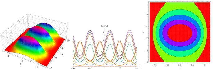
Numerical simulation of Eq. (13) in three distinct types of plots
-
2.
Fig. 2 shows the dark cone wave solution (14) in the three-dimensional plot (a) to explain the perspective view of the solution, the two-dimensional plot (b) to explain the wave propagation pattern of the wave along the x-axis, and the contour plot (c) to explain the overhead view of the solution when \({[} \alpha=\frac {1}{2}, \delta=6, \lambda=3, m=1, n=1, \chi=5, \varrho=1 {]}\).
Figure 2 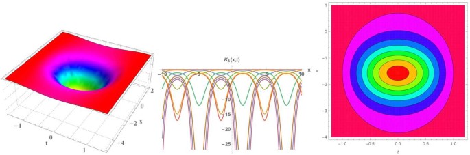
Numerical simulation of Eq. (14) in three distinct types of plots
-
3.
Fig. 3 shows the periodic bright cone-wave solution (40) in the three-dimensional plot (a) to explain the perspective view of the solution, the two-dimensional plot (b) to explain the wave propagation pattern of the wave along the x-axis, and the contour plot (c) to explain the overhead view of the solution when \({[} \alpha=\frac{1}{2}, \delta=6, \lambda=3, m=1, n=1, \chi=5, \varrho=1 {]}\).
Figure 3 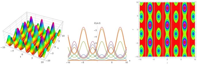
Numerical simulation of Eq. (40) in three distinct types of plots
-
4.
Fig. 4 shows the cone-wave solution (43) in the three-dimensional plot (a) to explain the perspective view of the solution, the two-dimensional plot (b) to explain the wave propagation pattern of the wave along the x-axis, and the contour plot (c) to explain the overhead view of the solution when \({[} \alpha=\frac {1}{2}, \delta=-9, \lambda=3, m=1, n=1, \chi=0, \varrho=1 {]}\).
Figure 4 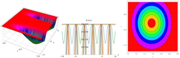
Numerical simulation of Eq. (43) in three distinct types of plots


4 Results and discussion
This section is divided into two main parts. In the first part, we studyg the obtained computational solutions for the two fractional suggested models. whereas in the second part, we compare them with the other obtained results in previous works.
-
1.
The shown solutions in our paper.
-
In this paper, we investigate the fractional KdV and ZKBBM equation by the employment of the mK method and a new fractional definition (\(\mathcal{ABR}\)). Abundant explicit closed-form solutions are obtained for each fractional model. Receptive twenty-six and twenty-eight solutions are obtained for each mentioned fractional model.
-
-
2.
The solutions obtained in previous works.
-
In [56], two analytical methods are applied to three different models involving two our models. However, they use two schemes, but a very few special solutions are obtained.
-
Two analytical schemes in [56] are just particular cases of the mK method when \({[} \mathcal{Q}^{\mathcal{M}(\varphi )}= ( \frac{G'}{G} ), \varrho=-\mu, \chi=-\lambda, \delta=1 {]}\).
-
Eq. (27) is equal to Eq. (3.9) in [56] when \({[} e_{0}=-12 \delta(\mu+d (d-\lambda)), -3(\lambda^{2}-4 \mu )=\delta\lambda\varrho {]}\).
-
Eq. (43) is equal to Eq. (3.30) in [56] when \({[} B=0, a=v, c=2 b v \lambda^{2}-8 b V \mu+V, b V (\lambda^{2}-4 \mu)=-4 c \delta\mu\varrho {]}\).
-
All other solutions obtained in this paper are new when compared with those obtained in [56].
-
5 Conclusion
In our paper, we solved the flaws and disadvantages of the \(( \frac{G'}{G} ) \)-expansion method that is used by Ali Akbar et al. [56] because, as shown in the previous section, it is just a particular case of our method. Moreover, we use a new definition of fractional derivative, which successfully converts the fractional-order differential equations from our models to integer-order ordinary differential equations. Abundant new solutions for both models were obtained, and to further clarify the physical meaning of these solutions, some plots are sketched in three- and two-dimensional and contour plots (Figs. 1, 2, 3, 4).
References
Alderremy, A.A., Attia, R.A.M., Alzaidi, J.F., Lu, D., Khater, M.M.A.: Analytical and semi-analytical wave solutions for longitudinal wave equation via modified auxiliary equation method and Adomian decomposition method. Therm. Sci. 23, S1943–S1957 (2019)
Ali, A.T., Khater, M.M., Attia, R.A., Abdel-Aty, A.-H., Lu, D.: Abundant numerical and analytical solutions of the generalized formula of Hirota–Satsuma coupled KdV system. Chaos Solitons Fractals 131, Article ID 109473 (2020)
Arqub, O.A., El-Ajou, A., Momani, S.: Constructing and predicting solitary pattern solutions for nonlinear time-fractional dispersive partial differential equations. J. Comput. Phys. 293, 385–399 (2015)
Atangana, A., Gómez-Aguilar, J.F.: Numerical approximation of Riemann–Liouville definition of fractional derivative: from Riemann–Liouville to Atangana–Baleanu. Numer. Methods Partial Differ. Equ. 34(5), 1502–1523 (2018)
Atangana, A., Koca, I.: Chaos in a simple nonlinear system with Atangana–Baleanu derivatives with fractional order. Chaos Solitons Fractals 89, 447–454 (2016)
Attia, R.A., Lu, D., Khater, M.M.A.: Chaos and relativistic energy-momentum of the nonlinear time fractional Duffing equation. Math. Comput. Appl. 24(1), Article ID 10 (2019)
Baleanu, D., Agrawal, O.P.: Fractional Hamilton formalism within Caputo’s derivative. Czechoslov. J. Phys. 56(10–11), 1087–1092 (2006)
Baleanu, D., Muslih, S.I.: About Lagrangian formulation of classical fields within Riemann–Liouville fractional derivatives. In: ASME 2005 International Design Engineering Technical Conferences and Computers and Information in Engineering Conference, pp. 1457–1464 (2005)
Benci, V., Fortunato, D.F.: Solitary waves of the nonlinear Klein–Gordon equation coupled with the Maxwell equations. Rev. Math. Phys. 14(4), 409–420 (2002)
Fernandez, A., Özarslan, M.A., Baleanu, D.: On fractional calculus with general analytic kernels. Appl. Math. Comput. 354, 248–265 (2019)
Gao, W., Ghanbari, B., Günerhan, H., Baskonus, H.M.: Some mixed trigonometric complex soliton solutions to the perturbed nonlinear Schrödinger equation. Mod. Phys. Lett. B 34(3), Article ID 2050034 (2020)
Gepreel, K.A., Omran, S.: Exact solutions for nonlinear partial fractional differential equations. Chin. Phys. B 21(11), Article ID 110204 (2012)
Ghanbari, B., et al.: A new generalized exponential rational function method to find exact special solutions for the resonance nonlinear Schrödinger equation. Eur. Phys. J. Plus 133(4), Article ID 142 (2018)
Ghanbari, B., Baleanu, D.: New solutions of Gardner’s equation using two analytical methods. Front. Phys. 7, Article ID 202 (2019)
Ghanbari, B., Baleanu, D.: A novel technique to construct exact solutions for nonlinear partial differential equations. Eur. Phys. J. Plus 134(10), Article ID 506 (2019)
Ghanbari, B., Gómez-Aguilar, J.F.: New exact optical soliton solutions for nonlinear Schrödinger equation with second-order spatio-temporal dispersion involving M-derivative. Mod. Phys. Lett. B 33(20), Article ID 1950235 (2019)
Ghanbari, B., Kuo, C.-K.: New exact wave solutions of the variable-coefficient \((1+ 1)\)-dimensional Benjamin–Bona–Mahony and \((2+ 1)\)-dimensional asymmetric Nizhnik–Novikov–Veselov equations via the generalized exponential rational function method. Eur. Phys. J. Plus 134(7), Article ID 334 (2019)
Ghanbari, B., Osman, M.S., Baleanu, D.: Generalized exponential rational function method for extended Zakharov–Kuzetsov equation with conformable derivative. Mod. Phys. Lett. A 34(20), Article ID 1950155 (2019)
Ghanbari, B., Rada, L., et al.: Solitary wave solutions to the Tzitzeica type equations obtained by a new efficient approach. J. Appl. Anal. Comput. 9(2), 568–589 (2019)
Guo, M., Fu, C., Zhang, Y., Liu, J., Yang, H.: Study of ion–acoustic solitary waves in a magnetized plasma using the three-dimensional time–space fractional Schamel–KdV equation. Complexity 2018, Article ID 6852548 (2018)
He, J.-H.: Exp-function method for fractional differential equations. Int. J. Nonlinear Sci. Numer. Simul. 14(6), 363–366 (2013)
He, J.-H., Wu, X.-H.: Construction of solitary solution and compacton-like solution by variational iteration method. Chaos Solitons Fractals 29(1), 108–113 (2006)
Heymans, N., Podlubny, I.: Physical interpretation of initial conditions for fractional differential equations with Riemann–Liouville fractional derivatives. Rheol. Acta 45(5), 765–771 (2006)
Hilfer, R.: Fractional diffusion based on Riemann–Liouville fractional derivatives. J. Phys. Chem. B 104(16), 3914–3917 (2000)
Inc, M.: The approximate and exact solutions of the space- and time-fractional Burgers equations with initial conditions by variational iteration method. J. Math. Anal. Appl. 345(1), 476–484 (2008)
Khader, M.M., Saad, K.M.: On the numerical evaluation for studying the fractional KdV, KdV–Burgers and Burgers equations. Eur. Phys. J. Plus 133(8), 335 (2018)
Khater, M., Attia, R., Lu, D.: Modified auxiliary equation method versus three nonlinear fractional biological models in present explicit wave solutions. Math. Comput. Appl. 24(1), Article ID 1 (2019)
Khater, M., Attia, R.A., Lu, D.: Explicit lump solitary wave of certain interesting \((3+ 1)\)-dimensional waves in physics via some recent traveling wave methods. Entropy 21(4), Article ID 397 (2019)
Khater, M.M., Lu, D., Attia, R.A.: Dispersive long wave of nonlinear fractional Wu–Zhang system via a modified auxiliary equation method. AIP Adv. 9(2), Article ID 025003 (2019)
Khater, M.M., Lu, D., Attia, R.A.: Erratum: “Dispersive long wave of nonlinear fractional Wu–Zhang system via a modified auxiliary equation method” [AIP Adv. 9, 025003 (2019)]. AIP Adv. 9(4), Article ID 049902 (2019)
Khater, M.M., Lu, D., Attia, R.A.: Lump soliton wave solutions for the \((2+ 1)\)-dimensional Konopelchenko–Dubrovsky equation and KdV equation. Mod. Phys. Lett. B 33, Article ID 1950199 (2019)
Khater, M.M., Seadawy, A.R., Lu, D.: Elliptic and solitary wave solutions for Bogoyavlenskii equations system, couple Boiti–Leon–Pempinelli equations system and time-fractional Cahn–Allen equation. Results Phys. 7, 2325–2333 (2017)
Khater, M.M.A., Baleanu, D.: On new analytical and semi-analytical wave solutions of the quadratic–cubic fractional nonlinear Schrödinger equation. Chaos Solitons Fractals (2020, submitted)
Khater, M.M.A., Baleanu, D.: On the new explicit computational and numerical solutions of the fractional nonlinear space–time Telegraph equation. Mod. Phys. Lett. A (2020, submitted)
Kuo, C.-K., Ghanbari, B.: Resonant multi-soliton solutions to new \((3+ 1)\)-dimensional Jimbo–Miwa equations by applying the linear superposition principle. Nonlinear Dyn. 96(1), 459–464 (2019)
Kurulay, M., Bayram, M.: Approximate analytical solution for the fractional modified KdV by differential transform method. Commun. Nonlinear Sci. Numer. Simul. 15(7), 1777–1782 (2010)
Le, U., Pelinovsky, D.E.: Convergence of Petviashvili’s method near periodic waves in the fractional Korteweg–de Vries equation. SIAM J. Math. Anal. 51(4), 2850–2883 (2019)
Li, J., Qiu, Y., Lu, D., Attia, R.A.M., Khater, M.M.A.: Study on the solitary wave solutions of the ionic currents on microtubules equation by using the modified Khater method. Therm. Sci. 23, S2053–S2062 (2019)
Liu, Q., Zhang, R., Yang, L., Song, J.: A new model equation for nonlinear Rossby waves and some of its solutions. Phys. Lett. A 383(6), 514–525 (2019)
Liu, W., Chen, K.: The functional variable method for finding exact solutions of some nonlinear time-fractional differential equations. Pramana 81(3), 377–384 (2013)
Losada, J., Nieto, J.J.: Properties of a new fractional derivative without singular kernel. Prog. Fract. Differ. Appl. 1(2), 87–92 (2015)
Lu, C., Fu, C., Yang, H.: Time-fractional generalized Boussinesq equation for Rossby solitary waves with dissipation effect in stratified fluid and conservation laws as well as exact solutions. Appl. Math. Comput. 327, 104–116 (2018)
Luchko, Y., Gorenflo, R.: An operational method for solving fractional differential equations with the Caputo derivatives. Acta Math. Vietnam. 24(2), 207–233 (1999)
Osman, M.S., Ghanbari, B.: New optical solitary wave solutions of Fokas–Lenells equation in presence of perturbation terms by a novel approach. Optik 175, 328–333 (2018)
Osman, M.S., Ghanbari, B., Machado, J.A.T.: New complex waves in nonlinear optics based on the complex Ginzburg–Landau equation with Kerr law nonlinearity. Eur. Phys. J. Plus 134(1), Article ID 20 (2019)
Ray, S.S., Sahoo, S.: Invariant analysis and conservation laws of \((2+ 1)\) dimensional time-fractional ZK–BBM equation in gravity water waves. Comput. Math. Appl. 75(7), 2271–2279 (2018)
Rezazadeh, H., Korkmaz, A., Eslami, M., Vahidi, J., Asghari, R.: Traveling wave solution of conformable fractional generalized reaction Duffing model by generalized projective Riccati equation method. Opt. Quantum Electron. 50(3), Article ID 150 (2018)
Rezazadeh, H., Korkmaz, A., Khater, M.M., Eslami, M., Lu, D., Attia, R.A.: New exact traveling wave solutions of biological population model via the extended rational sinh–cosh method and the modified Khater method. Mod. Phys. Lett. B 33(28), Article ID 1950338 (2019)
Saad, K.M., Baleanu, D., Atangana, A.: New fractional derivatives applied to the Korteweg–de Vries and Korteweg–de Vries–Burger’s equations. Comput. Appl. Math. 37(4), 5203–5216 (2018)
Shah, N.A., Khan, I.: Heat transfer analysis in a second grade fluid over and oscillating vertical plate using fractional Caputo–Fabrizio derivatives. Eur. Phys. J. C 76(7), Article ID 362 (2016)
Sun, J.-C., Zhang, Z.-G., Dong, H.-H., Yang, H.-W.: Fractional order model and Lump solution in dusty plasma. Phys. J. 68(21), Article ID 210201 (2019)
Tian, R., Fu, L., Ren, Y., Yang, H.: \((3+ 1)\)-Dimensional time-fractional modified Burgers equation for dust ion-acoustic waves as well as its exact and numerical solutions. Math. Methods Appl. Sci. (2019). https://doi.org/10.1002/mma.5823
Yang, H., Fu, L., et al.: An application of \((3+ 1)\)-dimensional time–space fractional ZK model to analyze the complex dust acoustic waves. Complexity 2019, 1–15 (2019)
Yaro, D., Seadawy, A.R., Lu, D., Apeanti, W.O., Akuamoah, S.W.: Dispersive wave solutions of the nonlinear fractional Zakhorov–Kuznetsov–Benjamin–Bona–Mahony equation and fractional symmetric regularized long wave equation. Results Phys. 12, 1971–1979 (2019)
Yaslan, H.Ç., Girgin, A.: Exp-function method for the conformable space–time fractional STO, ZKBBM and coupled Boussinesq equations. Arab J. Basic Appl. Sci. 26(1), 163–170 (2019)
Zayed, E.M.E.: A generalized and improved \(({G}'/{G})\)-expansion method for nonlinear evolution equations. Math. Probl. Eng. 2012(3), Article ID 459879 (2012)
Zhang, R., Yang, L., Liu, Q., Yin, X.: Dynamics of nonlinear Rossby waves in zonally varying flow with spatial-temporal varying topography. Appl. Math. Comput. 346, 666–679 (2019)
Acknowledgements
MK would like to dedicate this paper to my mother, son (Adam), and the soul of my father. Their love, support, and constant care will never be forgotten.
Availability of data and materials
All data generated or analyzed during this study are included in the paper.
Funding
Not applicable.
Author information
Authors and Affiliations
Contributions
All authors conceived of the study, participated in its design and coordination, drafted the manuscript, participated in the sequence alignment, and read and approved the final manuscript.
Corresponding authors
Ethics declarations
Competing interests
The authors declare that they have no competing interests.
Rights and permissions
Open Access This article is licensed under a Creative Commons Attribution 4.0 International License, which permits use, sharing, adaptation, distribution and reproduction in any medium or format, as long as you give appropriate credit to the original author(s) and the source, provide a link to the Creative Commons licence, and indicate if changes were made. The images or other third party material in this article are included in the article’s Creative Commons licence, unless indicated otherwise in a credit line to the material. If material is not included in the article’s Creative Commons licence and your intended use is not permitted by statutory regulation or exceeds the permitted use, you will need to obtain permission directly from the copyright holder. To view a copy of this licence, visit http://creativecommons.org/licenses/by/4.0/.
About this article

Cite this article
Khater, M.M.A., Baleanu, D. On abundant new solutions of two fractional complex models. Adv Differ Equ 2020, 268 (2020). https://doi.org/10.1186/s13662-020-02705-x
Received:
Accepted:
Published:
DOI: https://doi.org/10.1186/s13662-020-02705-x