
Abstract
Teleparallel Horndeski theory offers an avenue through which to circumvent the speed constraint of gravitational waves in an efficient manner. However, this provides an even larger plethora of models due to the increase in action terms. In this work we explore these models in the context of cosmological systems. Using Noether point symmetries, we classify the dynamical systems that emerge from teleparallel Horndeski cosmologies. This approach is very effective at selecting specific models in the general class of second-order teleparallel scalar–tensor theories, as well as for deriving exact solutions within a cosmological context. By iterating through the Lagrangians selected through the Noether symmetries, we solve for a number of cosmological systems which provides new cosmological systems to be studied.
1 Introduction
General relativity (GR) as the fundamental theory that describes gravity in the standard model of cosmology (\(\Lambda \)CDM) has seen overwhelming successes in describing the evolutionary processes in the Universe [1,2,3]. In this scenario, the current phase of expansion is being driven by the vacuum energy associated with spacetime [4, 5]. However, fundamental issues remain prevalent for a cosmological constant \(\Lambda \) scenario [6,7,8]. Along a similar vein, the prospect of direct observations of cold dark matter (CDM) particles remains elusive [9, 10]. More recently, \(\Lambda \)CDM has been met by challenges from observational cosmology in the form of the Hubble tension [11,12,13,14] where a disagreement in the value of the Hubble constant has appeared between late-time cosmology-independent measurements of \(H_0\) [15, 16] in contrast to observations from the early Universe which are then used to predict the value of \(H_0\) using \(\Lambda \)CDM [3, 17].
In order to better meet these challenges, a possible solution may be to reconsider GR as the fundamental description of gravitation within the standard model of cosmology [2, 18,19,20]. The possible directions that theories modified beyond GR can take has branched out into several directions over the years with the Lovelock theorem as one key guide [21] in these studies. One of these proposals is the addition of a single nonminimally coupled scalar field to the Einstein–Hilbert action which has led to the umbrella of Horndeski gravity [22] which is dynamically equivalent to most modified theories of gravity in curvature-based scenarios. Horndeski gravity is a rich arena for constructing cosmological models [23]. However, recent multimessenger signals have put tight constraints on the speed of gravitational waves of at most one part in \(10^{15}\) in comparison with the speed of light [24, 25]. This has led to a severely restricted form of regular Horndeski gravity that continues to be observationally viable [26].
This adds a strong motivation to consider possible alternatives that may revitalize the search for a viable model in terms of phenomenological within this framework. One such possibility is the transformation from curvature- to torsion-based theories of gravity [27,28,29,30]. In this setting, we consider teleparallel gravity (TG) which embodies the exchange of the Levi-Civita to the teleparallel connection [27, 31], which is torsion-full but continues to satisfy metricity. This represents a transformation in the geometry of the theory and thus the regular measures of curvature identically vanish, such as the Ricci scalar  (over-circles represent quantities calculated with the Levi-Civita connection), which in TG gives \(R \equiv 0\). By relating both geometries, it can is found that the regular Ricci scalar is dynamically equal to a torsion scalar T, up to a boundary term B. This guarantees that GR is dynamically equivalent to a teleparallel equivalent of general relativity (TEGR). Thus, in TG the division between the second- and fourth-order contributions to the Einstein–Hilbert action are decoupled which produces a softened version of the Lovelock theorem in this setting [21, 32, 33].
TEGR can be generalized in a number of interesting ways, using the same reasoning as  [18, 34,35,36] we can consider f(T) gravity [37,38,39,40,41,42], or even f(T, B) gravity [43,44,45,46,47,48,49,50] which have both shown interesting results in the literature. Another interesting generalization of TEGR that has gained interest in the literature is that of using the teleparallel analogue of the Gauss–Bonnet scalar \(T_G\) which can be used to produce \(f(T,T_G)\) gravity [51,52,53,54]. A novel approach in this direction has been recently suggested in Ref. [33] where a TG analogue of Horndeski theory was developed. Due to the organically lower order nature of TG, this produces a much richer landscape in which to produce scalar–tensor models. This inadvertently also helps revive previously disqualified models since the gravitational wave propagation equation becomes much more intricate [55]. Most models in the teleparallel Horndeski theory also satisfy the parameterized post-Newtonian conditions [56] and produce a varied polarization structure for gravitational waves [57]. More recently, teleparallel Horndeski gravity has been studied for its self-tuning properties in Refs. [58, 59].
In this work, we aim to use the Noether symmetry approach [60] to classify the ensuing models that can be produced within the teleparallel Horndeski plethora of models. This approach is a vital tool to probing physical models of a landscape of scalar–tensor theories such as Horndeski gravity since it can use symmetries to reduce the complexity of a system of equations [61]. In practice, the method depends on a point-like Lagrangian and a symmetry that leaves the Lagrangian invariant, which are then used to reduce the complexity for a systems so that analytic solutions may potentially be found [62]. These symmetries are always connected with conserved quantities in a system under investigation. Now, this investigative technique has been used in several settings [63] such as  [64, 65], scalar–tensor theories [66,67,68,69], as well as non-local theories [70]. In TG, this has been used in f(T) gravity [71], f(T, B) gravity [46] and \(f(T,T_G)\) gravity [72]. As an approach of classification of theories in regular Horndeski gravity, this approach was presented in Ref. [73] where only the invariance of the field equations under a Noether point symmetry was considered. This work also led to a number of interesting new solutions. In the present work, we generalize this approach to teleparallel Horndeski gravity to broaden this classification approach and to obtain novel solutions.
Our study first opens with a brief discussion of TG and the construction of the teleparallel analogue of Horndeski gravity which takes place in Sect. 2. We then discuss our use of the Noether symmetry approach in Sect. 3 where our point-like Lagrangian is written down together with the Noether symmetries that are then investigated. In Sect. 4 we use the Noether symmetry approach for the point-like Lagrangian to classify the ensuing classes of models that emerge. Here, we discuss how the regular Horndeski models are complemented by the new additions from this larger form of Horndeski gravity. Finally, we give a summary of our main results in Sect. 5.
2 Teleparallel Horndeski cosmology
The curvature associated with GR is recast in TG with the torsional geometric framework offered by the teleparallel connection which replaces the Levi-Civita connection for gravitational interactions [27,28,29,30]. By reconsidering the foundations of GR, TG can offer an alternative approach by which to construct gravitational theories.
In TG the metric tensor is replaced as the fundamental dynamical variable by the tetrad \(e^{A}_{\,\mu }\) and spin connection \(\omega ^{B}_{\,C\nu }\), where Greek indices refer to coordinates on the general manifold while Latin ones represent local Minkowski space \(\eta _{AB}\). In this way, the tetrads can be used to raise Minkowski indices to the general manifold through [74]
which also adhere to orthogonality conditions
where \(E_{A}^{\,\mu }\) represents the inverse tetrad. Given a metric, there exists an infinite number of the tetrad components that satisfy these relations due to the six local Lorentz degrees of freedom \(\Lambda ^{A}_{\,B}\). These degrees of freedom are represented by the spin connection. Together, the tetrad-spin connection pair represented the fundamental variables of the theory.
The Levi-Civita connection  (to recall, over-circles refer to any quantities based on the Levi-Civita connection) associated with curvature-based theories is replaced in TG with the teleparallel connection \(\Gamma ^{\sigma }_{\,\mu \nu }\). This can also be done in GR but is much less common [75]. The teleparallel connection is curvature-less and satisfies metricity [31], and can be expressed as [29, 30]
where the spin connection must satisfy [27]
in order to be the flat connection associated with TG. In this way, the tetrad-spin connection pair balance each other in terms of the freedom of theory. It is important to point out that tetrad frames exist which are compatible with zero spin connection components (as long as they satisfy the corresponding field equations). This is called Weitzenböck gauge [30].
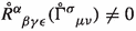
Teleparallel geometry is based on the replacement of the Levi-Civita with the teleparallel connection, which means that the Riemann tensor identically vanishes (\(R^{\alpha }_{\,\beta \gamma \epsilon }(\Gamma ^{\sigma }_{\,\mu \nu }) \equiv 0\)).Footnote 1 Thus, we consider the torsion tensor which is defined through the antisymmetry operator on the connection [28, 76]
which acts as a measure of the field strength of gravitation in TG [27], and where the square brackets denote antisymmetric operator. The torsion tensor transforms covariantly under local Lorentz transformations and diffeomorphisms [77], and can be decomposed into irreducible pieces, namely axial, vector and purely tensorial parts given by [78, 79]
where \(\epsilon _{\mu \nu \lambda \rho }\) is the totally antisymmetric Levi-Civita tensor in four dimensions. Naturally, when contracted with each other these irreducible parts vanish. This decomposition can also be used to form parts of the torsion scalar invariant through the scalars
which are parity preserving [44]. These three scalars form the most general gravitational Lagrangian formed only by parity preserving scalars, \(f(T_{\text {ax}},T_{\text {vec}},T_{\text {ten}})\), that is quadratic in contractions of the torsion tensor. Together, the torsion scalar can be formed by
which can be shown to be equivalent to the Ricci scalar  up to a total divergence term [44]

where R is the teleparallel connection calculated Ricci scalar (which identically vanishes since the teleparallel connection is curvature-less), \(e=\text {det}\left( e^{A}_{\,\mu }\right) =\sqrt{-g}\) is the tetrad determinant. The total divergence term defined the boundary quantity B through

The boundary term nature of B guarantees that an action formed by a linear contribution of T will produce a teleparallel 3 equivalent of general relativity (TEGR) [28, 80], while modifications of this may produce novel constructions of gravity [27, 29].
The equivalence principle offers a procedure by which to relate local Minkowski frames and the general manifold in GR. TG is not dissimilar in that the gravitational sector is indeed formed by the teleparallel connection but its interaction with matter preserves the minimal coupling prescription, namely [28, 81]

where partial derivatives are raised to the regular Levi-Civita covariant derivative for matter fields. Thus, both the gravitational and scalar field sectors are developed enough to consider the recently proposed teleparallel analog of Horndeski gravity [33, 55, 56], also called Bahamonde–Dialektopoulos–Levi Said (BDLS) theory. This construction of gravity in this framework depends on three limiting conditions which arise due to the organically lower-order nature of TG, namely (i) the field equations must be at most second order in their derivatives of the tetrads; (ii) the scalar invariants will not be parity violating; and (iii) the number of contractions with the torsion tensor is limited to being at most quadratic. Without these three conditions, the theory will admit an infinite number of terms which may not contribute appreciably to the physics. Automatically, this implies a weaker form of the generalized Lovelock theorem [21, 32, 82].
The teleparallel analog of Horndeski gravity or BDLS conditions leads directly to a finite number of contributing scalar invariants, which give the linearly coupled with the scalar field term [33]
where \(\phi \) is the scalar field, and while for the quadratic scenario, we find
where semicolons represent covariant derivatives with respect to the Levi-Civita connection. In addition the regular Horndeski Lagrangian terms (which can be calculating using the regular Levi-Civita connection due to the minimum coupling prescription) [22]


we also arrive at the additional term [33]
where the kinetic term is defined as \(X{:}{=}-\frac{1}{2}\partial ^{\mu }\phi \partial _{\mu }\phi \), and where the theory action is represented by
with \({\mathcal {L}}_\mathrm{m}\) is the matter Lagrangian in the Jordan conformal frame, \(\kappa ^2{:}{=}8\pi G\),  is the standard Einstein tensor, and comma represents regular partial derivatives. We denote the gravitational Lagrangian as \({\mathcal {L}} = e\left( {\mathcal {L}}_{\mathrm{Tele}} + \sum _{i=2}^{5} {\mathcal {L}}_i\right) \). One small difference to the original form of Horndeski gravity is that the tetrad is being used to make the calculations rather than the metric, but the resulting terms will be identical for the \({\mathcal {L}}_{2} - {\mathcal {L}}_{5}\) contributions. Clearly, the standard form of Horndeski gravity is recovered for the limit where \(G_{{\mathrm{Tele}}} = 0\). Another important point is that due to the invariance under local Lorentz transformations and diffeomorphisms, BDLS theory will also be invariant under these transformations.
3 Noether symmetries
Cosmological models identified through Noether symmetries offer an interesting approach by which to produce candidate models for further investigation. In this section, we present the teleparallel Horndeski Lagrangian followed by a brief review of the Noether approach to producing such cosmological solutions.
3.1 The point-like Lagrangian
Here, we will construct the point-like Lagrangian for the Lagrangian in Eq. (28) given a spatially flat Friedmann–Lemaître–Robertson–Walker (FLRW) metric. To this end, our core task is to incorporate the new torsion scalars into the formulation of the Lagrangian. This generalizes previous works on the topic [73] rendering a much more general set of solutions. Indeed, as will be explored in the Sect. 4 this will pose a problem in terms of the presentation of these solutions.
Consider the spatially flat FLRW metric described by
where N(t) represents the lapse function and a(t) the scale factor. This represents the maximally symmetric metric for this spacetime and thus can be used to produce the ensuing equations of motion. Aside from this, the scalar field \(\phi \) inherits all the symmetries of the spacetime, namely the position-independence \(\phi =\phi \;(t)\).
The metric in Eq. (29) can be reproduced by the tetrad \(e^{A}_{\,\mu } = \text {diag}(N(t),a(t),a(t),a(t))\) which turns out to be compatible with the Weitzenböck gauge [27], meaning a vanishing spin connection. Now, we consider the scalar contributions to the point-like Lagrangian by first calculating the torsion scalar
which is the Lagrangian density for TEGR. The only linear contraction scalar (16) is then given by
Interestingly, all the quadratic contraction scalars (17)–(22) vanish since only the vector irreducible is nonzero for this tetrad.
For completeness we also show the other scalars that are used to form the point-like Lagrangian where the derivative operators on the scalar field produce


while the kinetic term and the Ricci scalar are given by

Additionally, we apply the Lagrangian multiplier approach to the point-like Lagrangian by introducing the multipliers \(\lambda _1\) and \(\lambda _2\) which correspond to the scalars T and \(I_2\) respectively. The reasoning behind the use of Lagrangian multipliers is to identify any possible problematic features that may appear in the behaviour of the model. Moreover, this will provide a more convenient approach to investigating the properties of the theory more effectively.
By incorporating the Lagrangian multipliers as well as the scalar substitutions into the teleparallel Horndeski Lagrangian, we determine the point-like Lagrangian to be
For this setting, the Lagrangian coordinates are \(a(t),\phi (t),N(t),T(t),I_2(t)\) which implies a configuration space setup \(Q=(a,\phi ,N,T,I_2)\). Another feature of this Lagrangian is that the second-order derivatives can readily be eliminated through integration by parts. On the other hand, the only problematic term in this process is the \(a^3{\ddot{\phi }}\;G_3/N\) contribution which fails to be taken away using this approach. In order to resolve this issue, a reasonable choice is made in which we set
While not physically motivated, the choice that \(G_{3XX}=0\) provides a route by which most of the physically interesting and well-posed formulations can be derived. On this point, observational data cannot yet differentiate between the plethora of models available, and so we pursue the set of models that result from this setting providing a new range of possible cosmological models to probe.
Hence, the point-like Lagrangian in this setting is given by
which is the minimal form of the teleparallel Horndeski in this setting.
3.2 Noether symmetries
We briefly review how a general differential equation behaves under the action of a point transformation. Consider a system governed by a Lagrangian \({\mathcal {L}}\) with n generalized coordinates \(q^i\) and an independent variable t. The general form of an infinitesimal transformation acting on that system is expressed as follows.
Suppose that the dynamics of a system are governed by a Lagrangian \({\mathcal {L}}\) in terms of n generalized coordinates \(q^i\) while t is the independent variable.
which can be encapsulated in the generator vector of the transformation
For any differentiable function F, the action of this transformation is given by
which can readily be extended for the case where F also has a velocity dependence
where
is the first prolongation of the generator vector. For the case in which \(F = F(t,q,{\dot{q}},{\ddot{q}})\), the second prolongation will be applied giving
and so on for the nth order time derivative of q.
For the system under study consider the Lagrangian \({\mathcal {L}} = {\mathcal {L}}(t,q,{\dot{q}})\), the action of the system is said to invariant under infinitesimal transformations (up to a total divergence term), if the Rund–Trautman identity holds, namely [61]
where \({\mathcal {X}}^{(1)}\) is the first prolongation of the generating vector. Then, the generator vector \({\mathcal {X}}\) is a Noether symmetry of the dynamical system described by \({\mathcal {L}}\). For any such Noether symmetry, there exists a function
which is a first integral of the equations of motion. In the following, we will give explicit examples of the above general scenario.
4 Classification of teleparallel Horndeski cosmologies
For our configuration space, namely \(Q=(a,\phi ,N,T,I_2)\), of the point-like Lagrangian in Eq. (38), together with the independent variable of cosmic time t, the generator vector is described by
By applying the Rund–Trautman identity in Eq. (45) to the point-like Lagrangian (38) produces 62 differential equations for the coefficients of the Noether vector \(\xi ,\eta _a,\eta _{\phi },\eta _N,\eta _T,\eta _{I_2},f\) and the arbitrary Lagrangian functions \(G_i(\phi ,X)\). As already discussed, the Lagrangian functions are not all independent of each other [33, 55, 56] and may feature some overlap.
Considerations from Noether symmetries alone are not necessarily enough to fully determine \(G_i(\phi ,X)\) models. In some works, specific forms of the \(G_i(\phi ,X)\) functions are assumed in standard Horndeski theories [66,67,68,69] which aides in the full determination of cosmological models, as well as the Noether vector coefficients. Our strategy is rather to consider the most general Lagrangian and to constrain as much as possible the unknown functions of the model Lagrangian and Noether vector coefficients. This involves treating the symmetries in the most general way possible and investigating each possible symmetry in turn. This will produce particular models for the various scenarios that are produced in the teleparallel analogue of Horndeski gravity. In our case, if at least one coefficient of the generating Noether vector is nonzero, then a Noether symmetry is said to exist. The existence of such symmetries leads to different forms of the \(G_i(\phi ,X)\) functions which may be physically interesting.
In this work we exhaustively explored every possible cases that arise from considering the Noether symmetries as applied to the teleparallel analogue of Horndeski gravity. These symmetries are determined by the system of equations that come about by using the point-like Lagrangian (38) in conjunction with the Noether condition in Eq. (45) which leads to the over-constrained system of 62 equations. Now, these solutions are impacted by whether the \(g(\phi )\) function is vanishing or not in the redefinition in Eq. (37), this leads to genuinely distinct solutions. Moreover, the Noether classification cases result by considering the vanishes or not of each Noether vector coefficient, which lead to distinct solutions in most cases. The enormity of the teleparallel analogue of Horndeski gravity means that this process will result in many cases some of which may involve lengthy solutions not appropriate for such a setting. For this reason, we show below four specific examples of these cases, and retain the full set of classification case solutions separately.Footnote 2
Case 1 (2.a.ii.1.a.i.1.b.i.1.b in Table 2a):
In this first example, we find a solution to the 62 differential equations in which the Noether coefficients turn out to be
while the BDLS model functions are given by
which satisfies, as all the cases in the work, the speed constraint of gravitation waves [55]. In this and the other classification cases, the denominators cannot vanish due to the particular case not allowing it. This renders each case safe from divergences. This is an interesting case where the \(G_4\) functional expresses some dependence on the kinetic while the \(G_5\) function is nonzero. This is balanced by an intricate form of \(G_{ \mathrm{Tele}}\) which now must contain several terms to satisfy the gravitational wave constraint condition. It is difficult to relate these models to their standard Horndeski analogue since they do not regularly allow for so much of the dynamics to feature in the \(G_5\) function. On the other hand, we do note the dependence \(G_5 = G_5 (\phi )\) which omits the kinetic term, while the other functions do feature this term.
Case 2 (2.a.ii.1.a.ii.2.a.ii in Table 2a):
In other case of the solutions of the two differential equations, we find the Noether coefficients have values
where some of these results remain very general, and where the BDLS model functions now take on the form
This case is different because the \(G_5\) function is fully determined to be a constant while the \(G_4\) functional does not depend on the kinetic term. To that end, these parts of the model would survive the gravitational wave speed constraint in standard Horndeski gravity. The BDLS correction term then adds news dynamics distinct to this standard Horndeski model. What is interesting in this case is that the \(G_{ \mathrm{Tele}}\) term inherits directly the functional from the \(G_2\) term producing a coupling between the basic standard term and the BDLS correction term.
Case 3 (2.b.i2.b.ii.2.b.ii.2 in Table 2b):
In a similar vein, the generality of the \(G_2\) functional and the independence of \(G_4\) from the kinetic term remains the case with this case in which the Noether coefficients assume the values
while the Horndeski functions take the form
This case generalizes the \(G_5\) functional to arbitrary dependence on the scalar field, while also putting some kinetic term dependence on the \(G_4\) term. This is an example of a model that satisfies the gravitational wave constraint for BDLS theory but not for standard Horndeski gravity. As in the previous two cases, there is an \(I_2\) dependence on \(G_{ \mathrm{Tele}}\), together with a coupling with both \(G_4\)and \(G_5\) functionals.
Case 4 (2.b.ii1.a.ii.2.b.i in Table 2b):
The final case we consider that solves the 62 differential equations of the Noether symmetries gives
where the model functionals take the form
As in case 3, one of the Noether coefficients vanishes making the system slightly easier to solve. Here, we again observe nonvanishing \(G_4\) and \(G_5\) showing another case which is only possible, in an observationally consistent manner, in BDLS as compared with standard Horndeski theory.
5 Conclusions
Horndeski gravity is the most general scalar–tensor framework giving to second-order field equations [22]. Its teleparallel analogue [33] offers a larger framework in which to construct model since torsion naturally produces lower-order theories of gravity. The teleparallel of Horndeski gravity [55] is especially interesting because provides a direct way to circumvent the recent speed constraint on the propagation of gravitational waves [26]. Moreover it is well known that most higher order theories in curvature-based gravity can be mapped onto a dynamically equivalent Horndeski model, it follows that the teleparallel analogue allows for even more higher order dynamically equivalent theories. For these reasons, in this work, we studied the symmetries that emerge from the Noether symmetry approach. When such symmetries arise, the equations of motion become reducible and solvable in most cases. This means that exact solutions, which are rare in general, become more obtainable within this approach.
We do this by first determining the point-like Lagrangian for our setting in Sect. 3.1 using the maximally symmetric form of the flat FLRW metric. This is performed using a tetrad that is compatible with the Weitzenböck gauge. We then remove second-order derivatives in this Lagrangian using integration by parts. However, one of the terms, related to \(G_3\) poses a problem for this procedure and so we take the still general form of Eq. (37) for its functional form. In the end, this produced the point-like Lagrangian in Eq. (38) where the second-order derivatives have been removed. We then lay out the general approach taken in the remainder of the work in Sect. 3.2 where the first order equation of motion that emerges out of the Noether symmetry is given.
Thus, by applying the Rund–Trautman identity in Eq. (45) to the point-like Lagrangian (38) we find a system of 62 differential equations for the Noether vector coefficients and model functionals. This in turn leads to a large number of cases of this general system of equations. Given the enormity of these cases we display them elsewhere (GitHub). Saying that, in Sect. 4 we showcase 4 of these cases which display the power of this approach. To varying degrees, these cases give a determined system of model functionals and Noether symmetry coefficients. To display some information about the remainder of the other cases we present Tables in Appendix A where all the solution scenarios are enumerated together with the conditions which defines them. These are divided by whether the \(G_{4,XX}\) vanishes or not which is then subdivided into subcases.
These tables show the complexity available through the teleparallel analogue of Horndeski gravity. Moreover, they provide a wealth of models which may provide interesting dynamics for further investigation. Given the breadth of classification cases, it would not be feasible to explore the cosmology that they instigate in a systematic way. However, it would be very interesting to consider the viable models further and to determine their cosmological evolution.
Data Availability Statement
This manuscript has associated data regarding calculations and solutions in a data repository. [Authors’ comment: All data of Noether symmetry solutions are included at https://github.com/jacksonsaid/BDLS_Noether_classification.git.]
Notes
Naturally, this does not mean that the regular Riemann tensor vanishes in general, i.e.
 .
.The full set of Noether symmetry solutions can be found at https://github.com/jacksonsaid/BDLS_Noether_classification.git.
 .
.References
C. Misner, K. Thorne, J. Wheeler, Gravitation. No. pt. 3 in Gravitation (W. H. Freeman, New York, 1973). https://books.google.com.mt/books?id=w4Gigq3tY1kC
T. Clifton, P.G. Ferreira, A. Padilla, C. Skordis, Modified gravity and cosmology. Phys. Rep. 513, 1–189 (2012). https://doi.org/10.1016/j.physrep.2012.01.001arXiv:1106.2476 [astro-ph.CO]
Planck Collaboration, N. Aghanim et al., Planck 2018 results. VI. Cosmological parameters. Astron. Astrophys. 641, A6 (2020). https://doi.org/10.1051/0004-6361/201833910. arXiv:1807.06209 [astro-ph.CO]
Supernova Search Team Collaboration, A.G. Riess et al., Observational evidence from supernovae for an accelerating universe and a cosmological constant. Astron. J. 116, 1009–1038 (1998). https://doi.org/10.1086/300499. arXiv:astro-ph/9805201
Supernova Cosmology Project Collaboration, S. Perlmutter et al., Measurements of Omega and Lambda from 42 high redshift supernovae. Astrophys. J. 517, 565–586 (1999). https://doi.org/10.1086/307221. arXiv:astro-ph/9812133
S. Weinberg, The cosmological constant problem. Rev. Mod. Phys. 61, 1–23 (1989). https://doi.org/10.1103/RevModPhys.61.1
S. Appleby, E.V. Linder, The well-tempered cosmological constant. JCAP 07, 034 (2018). https://doi.org/10.1088/1475-7516/2018/07/034arXiv:1805.00470 [gr-qc]
M. Ishak, Testing general relativity in cosmology. Living Rev. Relativ. 22(1), 1 (2019). https://doi.org/10.1007/s41114-018-0017-4arXiv:1806.10122 [astro-ph.CO]
L. Baudis, Dark matter detection. J. Phys. G43(4), 044001 (2016). https://doi.org/10.1088/0954-3899/43/4/044001
G. Bertone, D. Hooper, J. Silk, Particle dark matter: evidence, candidates and constraints. Phys. Rep. 405, 279–390 (2005). https://doi.org/10.1016/j.physrep.2004.08.031arXiv:hep-ph/0404175
J.L. Bernal, L. Verde, A.G. Riess, The trouble with \(H_0\). JCAP 10, 019 (2016). https://doi.org/10.1088/1475-7516/2016/10/019arXiv:1607.05617 [astro-ph.CO]
E. Di Valentino et al., Cosmology intertwined II: the hubble constant tension. arXiv:2008.11284 [astro-ph.CO]
E. Di Valentino, O. Mena, S. Pan, L. Visinelli, W. Yang, A. Melchiorri, D.F. Mota, A.G. Riess, J. Silk, In the realm of the Hubble tension—a review of solutions. arXiv:2103.01183 [astro-ph.CO]
A.G. Riess et al., A comprehensive measurement of the local value of the Hubble constant with 1 km/s/Mpc uncertainty from the hubble space telescope and the SH0ES team. arXiv:2112.04510 [astro-ph.CO]
A.G. Riess, S. Casertano, W. Yuan, L.M. Macri, D. Scolnic, Large Magellanic Cloud Cepheid standards provide a 1% foundation for the determination of the Hubble constant and stronger evidence for physics beyond \(\Lambda \)CDM. Astrophys. J. 876(1), 85 (2019). https://doi.org/10.3847/1538-4357/ab1422arXiv:1903.07603 [astro-ph.CO]
K.C. Wong et al., H0LiCOW-XIII. A 2.4 per cent measurement of H0 from lensed quasars: 5.3\({\sigma }\) tension between early- and late-Universe probes. Mon. Not. R. Astron. Soc. 498(1), 1420–1439 (2020). https://doi.org/10.1093/mnras/stz3094arXiv:1907.04869 [astro-ph.CO]
DES Collaboration, T.M.C. Abbott et al., Dark energy survey year 1 results: a precise H0 estimate from DES Y1, BAO, and D/H data. Mon. Not. R. Astron. Soc. 480(3), 3879–3888 (2018). https://doi.org/10.1093/mnras/sty1939. arXiv:1711.00403 [astro-ph.CO]
S. Capozziello, M. De Laurentis, Extended theories of gravity. Phys. Rep. 509, 167–321 (2011). https://doi.org/10.1016/j.physrep.2011.09.003arXiv:1108.6266 [gr-qc]
CANTATA Collaboration, E.N. Saridakis et al., Modified gravity and cosmology: an update by the CANTATA network. arXiv:2105.12582 [gr-qc]
S. Nojiri, S.D. Odintsov, Unified cosmic history in modified gravity: from F(R) theory to Lorentz non-invariant models. Phys. Rep. 505, 59–144 (2011). https://doi.org/10.1016/j.physrep.2011.04.001arXiv:1011.0544 [gr-qc]
D. Lovelock, The Einstein tensor and its generalizations. J. Math. Phys. 12, 498–501 (1971). https://doi.org/10.1063/1.1665613
G.W. Horndeski, Second-order scalar-tensor field equations in a four-dimensional space. Int. J. Theor. Phys. 10, 363–384 (1974). https://doi.org/10.1007/BF01807638
T. Kobayashi, Horndeski theory and beyond: a review. Rep. Prog. Phys. 82(8), 086901 (2019). https://doi.org/10.1088/1361-6633/ab2429arXiv:1901.07183 [gr-qc]
LIGO Scientific, Virgo Collaboration, B.P. Abbott et al., GW170817: observation of gravitational waves from a binary neutron star inspiral. Phys. Rev. Lett. 119(16), 161101 (2017). https://doi.org/10.1103/PhysRevLett.119.161101. arXiv:1710.05832 [gr-qc]
A. Goldstein et al., An ordinary short gamma-ray burst with extraordinary implications: Fermi-GBM detection of GRB 170817A. Astrophys. J. 848(2), L14 (2017). https://doi.org/10.3847/2041-8213/aa8f41arXiv:1710.05446 [astro-ph.HE]
J.M. Ezquiaga, M. Zumalacárregui, Dark energy in light of multi-messenger gravitational-wave astronomy. Front. Astron. Space Sci. 5, 44 (2018). https://doi.org/10.3389/fspas.2018.00044arXiv:1807.09241 [astro-ph.CO]
S. Bahamonde, K.F. Dialektopoulos, C. Escamilla-Rivera, G. Farrugia, V. Gakis, M. Hendry, M. Hohmann, J.L. Said, J. Mifsud, E. Di Valentino, Teleparallel gravity: from theory to cosmology. arXiv:2106.13793 [gr-qc]
R. Aldrovandi, J.G. Pereira, Teleparallel Gravity, vol. 173 (Springer, Dordrecht, 2013). https://doi.org/10.1007/978-94-007-5143-9
Y.-F. Cai, S. Capozziello, M. De Laurentis, E.N. Saridakis, f(T) teleparallel gravity and cosmology. Rep. Prog. Phys. 79(10), 106901 (2016). https://doi.org/10.1088/0034-4885/79/10/106901arXiv:1511.07586 [gr-qc]
M. Krssak, R. van den Hoogen, J. Pereira, C. Böhmer, A. Coley, Teleparallel theories of gravity: illuminating a fully invariant approach. Class. Quantum Gravity 36(18), 183001 (2019). https://doi.org/10.1088/1361-6382/ab2e1farXiv:1810.12932 [gr-qc]
R. Weitzenböck, Invariantentheorie (Noordhoff, Gronningen, 1923)
P. Gonzalez, Y. Vasquez, Teleparallel equivalent of Lovelock gravity. Phys. Rev. D 92(12), 124023 (2015). https://doi.org/10.1103/PhysRevD.92.124023arXiv:1508.01174 [hep-th]
S. Bahamonde, K.F. Dialektopoulos, J. Levi Said, Can Horndeski theory be recast using teleparallel gravity? Phys. Rev. D 100(6), 064018 (2019). https://doi.org/10.1103/PhysRevD.100.064018arXiv:1904.10791 [gr-qc]
T.P. Sotiriou, V. Faraoni, f(R) theories of gravity. Rev. Mod. Phys. 82, 451–497 (2010). https://doi.org/10.1103/RevModPhys.82.451arXiv:0805.1726 [gr-qc]
V. Faraoni, f(R) gravity: successes and challenges, in 18th SIGRAV Conference (2008). arXiv:0810.2602 [gr-qc]
S. Nojiri, S.D. Odintsov, V.K. Oikonomou, Modified gravity theories on a nutshell: inflation, bounce and late-time evolution. Phys. Rep. 692, 1–104 (2017). https://doi.org/10.1016/j.physrep.2017.06.001arXiv:1705.11098 [gr-qc]
R. Ferraro, F. Fiorini, Modified teleparallel gravity: inflation without an inflaton. Phys. Rev. D 75, 084031 (2007). https://doi.org/10.1103/PhysRevD.75.084031
R. Ferraro, F. Fiorini, On Born–Infeld gravity in Weitzenbock spacetime. Phys. Rev. D 78, 124019 (2008). https://doi.org/10.1103/PhysRevD.78.124019arXiv:0812.1981 [gr-qc]
G.R. Bengochea, R. Ferraro, Dark torsion as the cosmic speed-up. Phys. Rev. D 79, 124019 (2009). https://doi.org/10.1103/PhysRevD.79.124019arXiv:0812.1205 [astro-ph]
E.V. Linder, Einstein’s other gravity and the acceleration of the universe. Phys. Rev. D 81, 127301 (2010). https://doi.org/10.1103/PhysRevD.81.127301. arXiv:1005.3039 [astro-ph.CO]. [Erratum: Phys. Rev. D 82, 109902 (2010)]
S.-H. Chen, J.B. Dent, S. Dutta, E.N. Saridakis, Cosmological perturbations in f(T) gravity. Phys. Rev. D 83, 023508 (2011). https://doi.org/10.1103/PhysRevD.83.023508arXiv:1008.1250 [astro-ph.CO]
S. Bahamonde, K. Flathmann, C. Pfeifer, Photon sphere and perihelion shift in weak \(f(T)\) gravity. Phys. Rev. D 100(8), 084064 (2019). https://doi.org/10.1103/PhysRevD.100.084064arXiv:1907.10858 [gr-qc]
C. Escamilla-Rivera, J. Levi Said, Cosmological viable models in \(f(T, B)\) theory as solutions to the \(H_0\) tension. Class. Quantum Gravity 37(16), 165002 (2020). https://doi.org/10.1088/1361-6382/ab939carXiv:1909.10328 [gr-qc]
S. Bahamonde, C.G. Böhmer, M. Wright, Modified teleparallel theories of gravity. Phys. Rev. D 92(10), 104042 104042 (2015). https://doi.org/10.1103/PhysRevD.92.104042arXiv:1508.05120 [gr-qc]
S. Capozziello, M. Capriolo, M. Transirico, The gravitational energy–momentum pseudotensor: the cases of \(f(R)\) and \(f(T)\) gravity. Int. J. Geom. Methods Mod. Phys. 15, 1850164 (2018). https://doi.org/10.1142/S0219887818501645arXiv:1804.08530 [gr-qc]
S. Bahamonde, S. Capozziello, Noether symmetry approach in \(f(T, B)\) teleparallel cosmology. Eur. Phys. J. C 77(2), 107 (2017). https://doi.org/10.1140/epjc/s10052-017-4677-0arXiv:1612.01299 [gr-qc]
A. Paliathanasis, de Sitter and Scaling solutions in a higher-order modified teleparallel theory. JCAP 08, 027 (2017). https://doi.org/10.1088/1475-7516/2017/08/027arXiv:1706.02662 [gr-qc]
G. Farrugia, J. Levi Said, V. Gakis, E.N. Saridakis, Gravitational waves in modified teleparallel theories. Phys. Rev. D 97(12), 124064 (2018). https://doi.org/10.1103/PhysRevD.97.124064arXiv:1804.07365 [gr-qc]
S. Bahamonde, M. Zubair, G. Abbas, Thermodynamics and cosmological reconstruction in \(f(T, B)\) gravity. Phys. Dark Universe 19, 78–90 (2018). https://doi.org/10.1016/j.dark.2017.12.005arXiv:1609.08373 [gr-qc]
M. Wright, Conformal transformations in modified teleparallel theories of gravity revisited. Phys. Rev. D 93(10), 103002 (2016). https://doi.org/10.1103/PhysRevD.93.103002arXiv:1602.05764 [gr-qc]
G. Kofinas, E.N. Saridakis, Teleparallel equivalent of Gauss–Bonnet gravity and its modifications. Phys. Rev. D 90, 084044 084044 (2014). https://doi.org/10.1103/PhysRevD.90.084044arXiv:1404.2249 [gr-qc]
S. Bahamonde, C.G. Böhmer, Modified teleparallel theories of gravity: Gauss–Bonnet and trace extensions. Eur. Phys. J. C 76(10), 578 (2016). https://doi.org/10.1140/epjc/s10052-016-4419-8arXiv:1606.05557 [gr-qc]
A. de la Cruz-Dombriz, G. Farrugia, J.L. Said, D. Saez-Gomez, Cosmological reconstructed solutions in extended teleparallel gravity theories with a teleparallel Gauss–Bonnet term. Class. Quantum Gravity 34(23), 235011 (2017). https://doi.org/10.1088/1361-6382/aa93c8arXiv:1705.03867 [gr-qc]
A. de la Cruz-Dombriz, G. Farrugia, J.L. Said, D. Sáez-Chillón Gómez, Cosmological bouncing solutions in extended teleparallel gravity theories. Phys. Rev. D 97(10), 104040104040 (2018). https://doi.org/10.1103/PhysRevD.97.104040arXiv:1801.10085 [gr-qc]
S. Bahamonde, K.F. Dialektopoulos, V. Gakis, J. Levi Said, Reviving Horndeski theory using teleparallel gravity after GW170817. Phys. Rev. D 101(8), 084060 (2020). https://doi.org/10.1103/PhysRevD.101.084060arXiv:1907.10057 [gr-qc]
S. Bahamonde, K.F. Dialektopoulos, M. Hohmann, J. LeviSaid, Post-Newtonian limit of teleparallel Horndeski gravity. Class. Quantum Gravity 38(2), 025006 (2020). https://doi.org/10.1088/1361-6382/abc441arXiv:2003.11554 [gr-qc]
S. Bahamonde, M. Caruana, K.F. Dialektopoulos, V. Gakis, M. Hohmann, J. Levi Said, E.N. Saridakis, J. Sultana, Gravitational wave propagation and polarizations in the teleparallel analog of Horndeski gravity. arXiv:2105.13243 [gr-qc]
R.C. Bernardo, J.L. Said, M. Caruana, S. Appleby, Well-tempered Minkowski solutions in teleparallel Horndeski theory. arXiv:2108.02500 [gr-qc]
R.C. Bernardo, J.L. Said, M. Caruana, S. Appleby, Well-tempered teleparallel Horndeski cosmology: a teleparallel variation to the cosmological constant problem. arXiv:2107.08762 [gr-qc]
S. Capozziello, R. De Ritis, C. Rubano, P. Scudellaro, Noether symmetries in cosmology. Riv. Nuovo Cim. 19N4, 1–114 (1996). https://doi.org/10.1007/BF02742992
S. Basilakos, M. Tsamparlis, A. Paliathanasis, Using the Noether symmetry approach to probe the nature of dark energy. Phys. Rev. D 83, 103512 (2011). https://doi.org/10.1103/PhysRevD.83.103512arXiv:1104.2980 [astro-ph.CO]
K.F. Dialektopoulos, T.S. Koivisto, S. Capozziello, Noether symmetries in symmetric teleparallel cosmology. Eur. Phys. J. C 79(7), 606 (2019). https://doi.org/10.1140/epjc/s10052-019-7106-8arXiv:1905.09019 [gr-qc]
K.F. Dialektopoulos, S. Capozziello, Noether symmetries as a geometric criterion to select theories of gravity. Int. J. Geom. Methods Mod. Phys. 15(supp01), 1840007 (2018). https://doi.org/10.1142/S0219887818400078arXiv:1808.03484 [gr-qc]
S. Capozziello, A. De Felice, f(R) cosmology by Noether’s symmetry. JCAP 08, 016 (2008). https://doi.org/10.1088/1475-7516/2008/08/016arXiv:0804.2163 [gr-qc]
A. Paliathanasis, M. Tsamparlis, S. Basilakos, Constraints and analytical solutions of \(f(R)\) theories of gravity using Noether symmetries. Phys. Rev. D 84, 123514 (2011). https://doi.org/10.1103/PhysRevD.84.123514arXiv:1111.4547 [astro-ph.CO]
N. Dimakis, A. Giacomini, A. Paliathanasis, Integrability from point symmetries in a family of cosmological Horndeski Lagrangians. Eur. Phys. J. C 77(7), 458 (2017). https://doi.org/10.1140/epjc/s10052-017-5029-9arXiv:1701.07554 [gr-qc]
N. Dimakis, A. Giacomini, S. Jamal, G. Leon, A. Paliathanasis, Noether symmetries and stability of ideal gas solutions in Galileon cosmology. Phys. Rev. D 95(6), 064031 (2017). https://doi.org/10.1103/PhysRevD.95.064031arXiv:1702.01603 [gr-qc]
A. Giacomini, S. Jamal, G. Leon, A. Paliathanasis, J. Saavedra, Dynamical analysis of an integrable cubic Galileon cosmological model. Phys. Rev. D 95(12), 124060 (2017). https://doi.org/10.1103/PhysRevD.95.124060arXiv:1703.05860 [gr-qc]
A. Paliathanasis, M. Tsamparlis, S. Basilakos, S. Capozziello, Scalar–tensor gravity cosmology: Noether symmetries and analytical solutions. Phys. Rev. D 89(6), 063532 (2014). https://doi.org/10.1103/PhysRevD.89.063532arXiv:1403.0332 [astro-ph.CO]
S. Bahamonde, S. Capozziello, K.F. Dialektopoulos, Constraining generalized non-local cosmology from Noether symmetries. Eur. Phys. J. C 77(11), 722 (2017). https://doi.org/10.1140/epjc/s10052-017-5283-xarXiv:1708.06310 [gr-qc]
S. Basilakos, S. Capozziello, M. De Laurentis, A. Paliathanasis, M. Tsamparlis, Noether symmetries and analytical solutions in \(f(T)\)-cosmology: a complete study. Phys. Rev. D 88, 103526 (2013). https://doi.org/10.1103/PhysRevD.88.103526arXiv:1311.2173 [gr-qc]
S. Capozziello, M. De Laurentis, K.F. Dialektopoulos, Noether symmetries in Gauss–Bonnet-teleparallel cosmology. Eur. Phys. J. C 76(11), 629 (2016). https://doi.org/10.1140/epjc/s10052-016-4491-0arXiv:1609.09289 [gr-qc]
S. Capozziello, K.F. Dialektopoulos, S.V. Sushkov, Classification of the Horndeski cosmologies via Noether symmetries. Eur. Phys. J. C 78(6), 447 (2018). https://doi.org/10.1140/epjc/s10052-018-5939-1arXiv:1803.01429 [gr-qc]
F.W. Hehl, P. von der Heyde, G.D. Kerlick, J.M. Nester, General relativity with spin and torsion: foundations and prospects. Rev. Mod. Phys. 48, 393–416 (1976). https://doi.org/10.1103/RevModPhys.48.393
M. Hohmann, Variational principles in teleparallel gravity theories. Universe 7(5), 114 (2021). https://doi.org/10.3390/universe7050114arXiv:2104.00536 [gr-qc]
T. Ortín, Gravity and Strings. Cambridge Monographs on Mathematical Physics (Cambridge University Press, Cambridge, 2004). https://books.google.com.mt/books?id=sRlHoXdAVNwC
M. Krššák, E.N. Saridakis, The covariant formulation of f(T) gravity. Class. Quantum Gravity 33(11), 115009 (2016). https://doi.org/10.1088/0264-9381/33/11/115009arXiv:1510.08432 [gr-qc]
K. Hayashi, T. Shirafuji, New general relativity. Phys. Rev. D 19, 3524–3553 (1979). https://doi.org/10.1103/PhysRevD.19.3524
S. Bahamonde, C.G. Böhmer, M. Krššák, New classes of modified teleparallel gravity models. Phys. Lett. B 775, 37–43 (2017). https://doi.org/10.1016/j.physletb.2017.10.026arXiv:1706.04920 [gr-qc]
F.W. Hehl, J.D. McCrea, E.W. Mielke, Y. Ne’eman, Metric affine gauge theory of gravity: field equations, Noether identities, world spinors, and breaking of dilation invariance. Phys. Rep. 258, 1–171 (1995). https://doi.org/10.1016/0370-1573(94)00111-FarXiv:gr-qc/9402012
J. Beltrán Jiménez, L. Heisenberg, T. Koivisto, The coupling of matter and spacetime geometry. Class. Quantum Gravity 37(19), 195013 (2020). https://doi.org/10.1088/1361-6382/aba31barXiv:2004.04606 [hep-th]
P. González, S. Reyes, Y. Vásquez, Teleparallel equivalent of Lovelock gravity, generalizations and cosmological applications. JCAP 07, 040 (2019). https://doi.org/10.1088/1475-7516/2019/07/040arXiv:1905.07633 [gr-qc]
Acknowledgements
KFD acknowledges support by the Hellenic Foundation for Research and Innovation (H.F.R.I.) under the “First Call for H.F.R.I. Research Projects to support Faculty members and Researchers and the procurement of high-cost research equipment grant” (Project Number: 2251). The authors would like to acknowledge networking support by the COST Action CA18108 and funding support from Cosmology@MALTA which is supported by the University of Malta. The authors would also like to acknowledge funding from “The Malta Council for Science and Technology” in project IPAS-2020-007.
Author information
Authors and Affiliations
Corresponding author
Appendix A: Noether classifications
Appendix A: Noether classifications
In the appendix we present on a table all the different classes of theories that appear through the classification process. Not all of them lead to symmetries because in some cases the system of equations was too complicated to be solved, or not all the functions are fully determined. In greater detail, meaning the Noether vector coefficients and the form of the \(G_i\) functions of the Lagrangian, can be found in the notebook files in GitHub.
\({\varvec{1. : G_{4,XX}\ne 0}}\)
\(\mathbf{1}\).a : \( \mathbf {h'(\phi )\ne 0}\) | \(\mathbf{1}\).b : \(\mathbf {h'(\phi )=0}\) | ||
|---|---|---|---|
1.a.i | \( G_{\mathrm{Tele },I_2 I_2}(\phi ,X,T,I_2)\ne 0\) | 1.b.i | \( G_{\mathrm{Tele},I_2 I_2}(\phi ,X,T,I_2)\ne 0\) |
1.a.ii | \(G_{\mathrm{Tele},I_2I_2} (\phi ,X,T,I_2)=0\) | 1.b.ii | \(G_{\mathrm{Tele},I_2I_2}(\phi ,X,T,I_2) =0\) |
1.a.ii.1 | \(G_{\mathrm{Tele}2,T}(\phi ,X,T)\ne 0\) | 1.b.ii.1 | \(G_{\mathrm{Tele}2,I_2I_2}(\phi ,X,I_2)\ne 0\) |
1.a.ii.2 | \(G_{\mathrm{Tele}2,T}(\phi ,X,T)=0\) | 1.b.ii.2 | \(G_{\mathrm{Tele}2,I_2I_2}(\phi ,X,I_2)=0\) |
\({\varvec{2. : G_{4,XX}= 0}}\)
\(\mathbf{2}\).a : \( \mathbf {G_{{Tele},{XI2}}(\phi ,X,T,I_2)\ne 2 G_{4b}'(\phi )-g(\phi )}\) | |
|---|---|
2.a.i. | \( G_{\mathrm{Tele},{XT}}(\phi ,X,T,I_2)\ne G_5'(\phi )\) |
2.a.i.1. | \(g(\phi )\ne 0\) |
2.a.i.1.a. | \(G_{\mathrm{Tele} 2a,{TT}}(\phi ,T)\ne -G_{\mathrm{Tele}1,{TT}} (\phi ,T,I2)\) |
2.a.i.1.b. | \(G_{\mathrm{Tele} 2a,{TT}}(\phi ,T)\,=\,-G_{\mathrm{Tele}1,{TT}} (\phi ,T,I2)\) |
2.a.i.1.b.i. | \( G_{\mathrm{Tele} 1b,{I_2}}(\phi ,I_2) \ne 0\) |
2.a.i.1.b.ii. | \( G_{\mathrm{Tele} 1b,{I_2}}(\phi ,I_2)=0\) |
2.a.i.1.b.ii.1. | \(G_{\mathrm{Tele} 3{T I_2}}(\phi ,I,I_2),\ne 0\) |
2.a.i.1.b.ii.2. | \(G_{\mathrm{Tele} 3,{T I_2}}(\phi ,I,I_2)=0\) |
2.a.i.1.b.ii.2.a. | \(G_{\mathrm{Tele} 2c,{TT} }(\phi ,T) \,+ \,G_{\mathrm{Tele} 3a,{TT}}(\phi ,T)\ne 0\) |
2.a.i.1.b.ii.2.b. | \(G_{\mathrm{Tele} 2c,{TT} }(\phi ,T)\,+ \,G_{\mathrm{Tele} 3a,{TT}}(\phi ,T)=0\) |
2.a.i.2. | \(g(\phi )=0\) |
2.a.i.2.a. | \(G_{4b}(\phi )\ne G_5'(\phi )/2\) |
2.a.i.2.a.i. | \(G_{\mathrm{Tele} 1,{I_2}}(\phi ,T,I_2)\ne 2 G_{4b}'(\phi )\) |
2.a.i.2.a.i.1. | \(h'(\phi )\ne 0\) |
2.a.i.2.a.i.1.a. | \(G_{\mathrm{Tele} 3,{I_2I_2}}(\phi ,T,I_2)\ne 0\) |
2.a.i.2.a.i.1.b. | \(G_{\mathrm{Tele} 3,{I_2I_2}}(\phi ,T,I_2)=0\) |
2.a.i.2.a.i.1.b.i. | \(G_{\mathrm{Tele} 3b,T}(\phi ,T)\ne 0\) |
2.a.i.2.a.i.1.b.ii. | \(G_{\mathrm{Tele} 3b,T}(\phi ,T)=0\) |
2.a.i.2.a.i.1.b.ii.1. | \(G_{\mathrm{Tele} 1,{TI_2}}(\phi ,T,I_2)\ne 0\) |
2.a.i.2.a.i.1.b.ii.2. | \(G_{\mathrm{Tele} 1,{TI_2}}(\phi ,T,I_2)=0\) |
2.a.i.2.a.i.1.b.ii.2.a | \(G_{\mathrm{Tele}1,{I_2I_2}}(\phi ,I_2)\ne 0\) |
2.a.i.2.a.i.1.b.ii.2.b | \(G_{\mathrm{Tele}1,{I_2I_2}}(\phi ,I_2)=0\) |
2.a.i.2.a.i.2. | \( h'(\phi )=0\) |
2.a.i.2.a.ii. | \(G_{\mathrm{Tele} 1,{I_2}}(\phi ,T,I_2)=2 G_{4b}'(\phi )\) |
2.a.i.2.a.ii.1. | \(G_{4b}(\phi )\ne c_2/h'(\phi )+G_5'(\phi )/2\) |
2.a.i.2.a.ii.1.a. | \(c_3\ne 0\) |
2.a.i.2.a.ii.1.b. | \(c_3=0\) |
2.a.i.2.a.ii.1.b.i | \(G_{\mathrm{Tele} 3,{I_2I_2}}(\phi ,T,I_2)\ne 0\) |
2.a.i.2.a.ii.1.b.ii | \(G_{\mathrm{Tele} 3,{I_2I_2}}(\phi ,T,I_2)=0\) |
2.a.i.2.a.ii.2. | \(G_{4b}(\phi )= c_2/G_{3h}'(\phi )+G_5'(\phi )/2\) |
2.a.i.2.a.ii.2.a | \(G_{\mathrm{Tele} 3,{I_2I_2}}(\phi ,T,I_2)\ne 0\) |
2.a.i.2.a.ii.2.b | \(G_{\mathrm{Tele} 3,{I_2I_2}}(\phi ,T,I_2)=0\) |
2.a.i.2.a.ii.2.b.i | \(G_{\mathrm{Tele} 3b,{T}}(\phi ,T)\ne 0\) |
2.a.i.2.a.ii.2.b.ii | \(G_{\mathrm{Tele} 3b,{T}}(\phi ,T)=0\) |
2.a.i.2.b. | \(G_{4b}(\phi )= G_5'(\phi )/2\) |
2.a.i.2.b.i | \(h'(\phi )\ne 0\) |
2.a.i.2.b.ii | \(h'(\phi )= 0\) |
2.a.ii. | \(G_{\mathrm{Tele},{XT}}(\phi ,X,T,I_2)= G_5'(\phi )\) |
2.a.ii.1. | \(g(\phi )\ne 0\) |
2.a.ii.1.a | \(G_{4b}(\phi )\ne G_5'(\phi )/2\) |
2.a.ii.1.a.i | \(G_{\mathrm{Tele}2,{TI_2}}(\phi ,T,I_2)\ne 0\) |
2.a.ii.1.a.i.1 | \(G_5'(\phi )\ne 0\) |
2.a.ii.1.a.i.1.a | \(G_{\mathrm{Tele}1,{XI_2}}\ne 2 G_{4b}'(\phi )\) |
2.a.ii.1.a.i.1.a.i | \(3 g(\phi )^2 +2g'(\phi )(- 2G_{4b}(\phi )+G_5'(\phi )) +g(\phi ) ( -6G_{4b}'(\phi )+ 3G_{\mathrm{Tele}1,{XI_2}}(\phi ,X,I_2))\ne 0\) |
2.a.ii.1.a.i.1.a.ii | \(3 g(\phi )^2 +2g'(\phi )(- 2G_{4b}(\phi )+G_5'(\phi )) +g(\phi ) ( -6G_{4b}'(\phi )+ 3G_{\mathrm{Tele}1,{XI_2}}(\phi ,X,I_2)) = 0\) |
2.a.ii.1.a.i.1.b | \(G_{\mathrm{Tele}1,{XI_2}}=2 G_{4b}'(\phi )\) |
2.a.ii.1.a.i.1.b.i | \(G_{4b}(\phi )\ne 3g(\phi )^2/4g'(\phi ) + G_{5}'(\phi )/2\) |
2.a.ii.1.a.i.1.b.i.1 | \(g'(\phi )\ne 0\) |
2.a.ii.1.a.i.1.b.i.1.a | \(c_2\ne -9/5\) |
2.a.ii.1.a.i.1.b.i.1.b | \(c_2=-9/5\) |
2.a.ii.1.a.i.1.b.i.2 | \(g'(\phi )=0\) |
2.a.ii.1.a.i.1.b.ii | \(G_{4b}(\phi )=3 g(\phi )^2/4 g'(\phi ) +G_5'(\phi )/2\) |
[XMLCONT]
2.a.ii.1.a.i.1.b.ii.1 | \(G_{\mathrm{Tele} 2}(\phi ,T,I_2)=-G_{\mathrm{Tele} 1b}(\phi ,I_2)+G_{\mathrm{Tele} 2a}(\phi ,T)+3 I_2 T g(\phi )^3/(4g'(\phi )^2) +2 I_2 G_{4a}'(\phi )\) |
+ \( I_2 g(\phi ) (-4X g'(\phi )-4h'(\phi )+T G_5'(\phi )+2 G_{2,X}(\phi ,X)+2 G_{\mathrm{Tele} 1a,X}(\phi ,X))\,/\,2\,g'(\phi )\) | |
2.a.ii.1.a.i.2 | \(G_5'(\phi )=0\) |
2.a.ii.1.a.i.2.a | \(G_{\mathrm{Tele} 1}(\phi ,X,I_2)\ne G_{\mathrm{Tele 1a}}(\phi ,X) + G_{\mathrm{Tele}1b}(\phi ,I_2)+2 I_2 X G_{4b}'(\phi )\) |
2.a.ii.1.a.i.2.a.i | \(G_{\mathrm{Tele} 1}\ne -I_2 X g(\phi )+G_{\mathrm{Tele} 1a}(\phi ,X)+G_{\mathrm{Tele} 1b}(\phi ,I_2)+4 I_2 X G_{4b}(\phi ) g'(\phi )/3 g(\phi )+2 X I_2 G_{4b}'(\phi )\) |
2.a.ii.1.a.i.2.a.ii | \(G_{\mathrm{Tele} 1}= -I_2 X g(\phi )+G_{\mathrm{Tele} 1a}(\phi ,X)+G_{\mathrm{Tele} 1b}(\phi ,I_2)+4 I_2 X G_{4b}(\phi ) g'(\phi )/3 g(\phi )+2 X I_2 G_{4b}'(\phi )\) |
2.a.ii.1.a.i.2.b | \(G_{\mathrm{Tele} 1}(\phi ,X,I_2)= G_{\mathrm{Tele 1a}}(\phi ,X) + G_{\mathrm{Tele}1b}(\phi ,I_2)+2 I_2 X G_{4b}'(\phi )\) |
2.a.ii.1.a.i.2.b.i | \(g'(\phi )\ne 0\) |
2.a.ii.1.a.i.2.b.i.1 | \(G_{\mathrm{Tele}2}(\phi ,T,I_2) = 3 T X g(\phi )^2-3 T g(\phi )G_{4a}'(\phi )\) |
+ \(2g'(\phi )(2TG_{4a}(\phi )-G_{\mathrm{Tele}1b}(\phi ,I_2)+G_{\mathrm{Tele}2a}(\phi ,I_2+3Tg(\phi )/(4g'(\phi ))))\) | |
2.a.ii.1.a.i.2.b.i.1.a | \(G_{\mathrm{Tele}2a}(\phi ,T,I_2) = G_{\mathrm{Tele}2a1}(\phi )+2(I_2+3Tg(\phi )/(4g'(\phi )))/(9T)(9TG_{4a}'(\phi )\) |
+ \((6I_2^2-6I_2(I_2+3Tg(\phi )/(4g'(\phi )))+2(I_2+3Tg(\phi )/(4g'(\phi )))^2-9TX)g(\phi )\) | |
\(-6h'(\phi )(-I_2+3Tg(\phi )/(4g'(\phi ))) +3(-I_2+3Tg(\phi )/(4g'(\phi )))(G_{2,X}(\phi ,X)+G_{\mathrm{Tele}1a,X}(\phi ,X)) )\) | |
2.a.ii.1.a.i.2.b.i.1.a.i | \(h(\phi ) = c_2 + c_3 g(\phi )\) |
2.a.ii.1.a.i.2.b.i.1.a.ii | \(h(\phi ) \ne c_2 + c_3 g(\phi )\) |
2.a.ii.1.a.i.2.b.i.1.b | \(G_{\mathrm{Tele}2a}(\phi ,T,I_2) \ne G_{\mathrm{Tele}2a1}(\phi )+2(I_2+3Tg(\phi )/(4g'(\phi )))/(9T)(9TG_{4a}'(\phi )\) |
+ \((6I_2^2-6I_2(I_2+3Tg(\phi )/(4g'(\phi )))+2(I_2+3Tg(\phi )/(4g'(\phi )))^2-9TX)g(\phi )\) | |
\(-6h'(\phi )(-I_2+3Tg(\phi )/(4g'(\phi ))) +3(-I_2+3Tg(\phi )/(4g'(\phi )))(G_{2,X}(\phi ,X)+G_{\mathrm{Tele}1a,X}(\phi ,X)) )\) | |
2.a.ii.1.a.i.2.b.i.2. | \(G_{\mathrm{Tele}2}(\phi ,T,I_2) \ne 3 T X g(\phi )^2-3 T g(\phi )G_{4a}'(\phi )\) |
+ \(2g'(\phi )(2TG_{4a}(\phi )-G_{\mathrm{Tele}1b}(\phi ,I_2)+G_{\mathrm{Tele}2a}(\phi ,I_2+3Tg(\phi )/(4g'(\phi ))))\) | |
2.a.ii.1.a.i.2.b.ii | \(g'(\phi )=0\) |
2.a.ii.1.a.i.2.b.ii.1 | \(G_{4b}(\phi )=c_2/h'(\phi )\) |
2.a.ii.1.a.i.2.b.ii.2 | \(G_{4b}(\phi )\ne c_2/h'(\phi )\) |
2.a.ii.1.a.ii | \(G_{\mathrm{Tele}2,{TI_2}}(\phi ,T,I_2)= 0\) |
2.a.ii.1.a.ii.1 | \(G_5'(\phi )\ne 0\) |
2.a.ii.1.a.ii.1.a | \(G_{\mathrm{Tele} 1},_{XI_2}\ne 2 G_{4b}'\) |
2.a.ii.1.a.ii.1.a.i | \(3 g^2(\phi )+2 g'(\phi ) ( -2 G_{4b}(\phi )+G_{5}'(\phi ) )+ g(\phi )( -6 G_{4b}'(\phi )+ 3 G_{\mathrm{Tele} 1}^{(0,1,1)}(\phi ,X,I_2))\ne 0\) |
2.a.ii.1.a.ii.1.a.i.1 | \(G_{\mathrm{Tele} 2a},_{TT}\ne 0\) |
2.a.ii.1.a.ii.1.a.i.2 | \(G_{\mathrm{Tele} 2a},_{TT}=0\) |
2.a.ii.1.a.ii.1.a.i.2.a | \(\eta _{\phi }(\phi )=0\) |
2.a.ii.1.a.ii.1.a.i.2.a.i | \(c_4\ne -1/2\) |
[XMLCONT]
2.a.ii.1.a.ii.1.a.i.2.a.i.1 | \(G_{4b}(\phi )=0\) |
2.a.ii.1.a.ii.1.a.i.2.a.i.2 | \(G_{4b}(\phi )\ne 0\) |
2.a.ii.1.a.ii.1.a.i.2.a.i.2.a | \(\eta _{I_2}(t,a,\phi ,N,T,I_2)\ne 0\) |
2.a.ii.1.a.ii.1.a.i.2.a.i.2.b | \(\eta _{I_2}(t,a,\phi ,N,T,I_2) = 0\) |
2.a.ii.1.a.ii.1.a.i.2.a.ii | \(c_4 = -1/2\) |
2.a.ii.1.a.ii.1.a.i.2.a.ii.1 | \(\eta _{a3c}\ne 0\) |
2.a.ii.1.a.ii.1.a.i.2.a.ii.2 | \(\eta _{a3c} = 0 \) |
2.a.ii.1.a.ii.1.a.i.2.a.ii.2.a | \(\eta _{I_2}(t,a,\phi ,N,T,I_2)\ne 0\) |
2.a.ii.1.a.ii.1.a.i.2.a.ii.2.b | \(\eta _{I_2}(t,a,\phi ,N,T,I_2) = 0\) |
2.a.ii.1.a.ii.1.a.i.2.b | \(\eta _{\phi }(\phi ) \ne 0\) |
2.a.ii.1.a.ii.1.a.i.2.b.i | \(G_{\mathrm{Tele} 1c}\ne -1/2\) |
2.a.ii.1.a.ii.1.a.i.2.b.i.1 | \(G_{\mathrm{Tele} 1c}\ne -2\) |
2.a.ii.1.a.ii.1.a.i.2.b.i.2 | \(G_{\mathrm{Tele} 1c}= -2\) |
2.a.ii.1.a.ii.1.a.i.2.b.ii | \(G_{\mathrm{Tele} 1c}= -1/2\) |
2.a.ii.1.a.ii.1.a.ii | \(3 g^2(\phi )+2 g'(\phi ) ( -2 G_{4b}(\phi )+G_{5}'(\phi ) )+ g(\phi )( -6 G_{4b}'(\phi )+ 3 G_{\mathrm{Tele} 1,XI_2}(\phi ,X,I_2))=0\) |
2.a.ii.1.a.ii.1.a.ii.1 | \(\eta _{\phi }(t,\phi ,N,I_2)=\eta _{\phi }(t,\phi )\) |
2.a.ii.1.a.ii.1.a.ii.1.a | \(\eta _{\phi }(t,\phi )\ne 0\) |
2.a.ii.1.a.ii.1.a.ii.1.b | \(\eta _{\phi }(t,\phi )=0 \) |
2.a.ii.1.a.ii.1.a.ii.1.b.i | \(G_{\mathrm{Tele} 2a,{TT}}(\phi ,T)\ne 0 \) |
2.a.ii.1.a.ii.1.a.ii.1.b.i.1 | \(G_{\mathrm{Tele} 2b}(\phi ,I_2) = -G_{\mathrm{Tele} 1b}(\phi ,I_2)+G_{\mathrm{Tele} 2b1}(\phi )+I_2 G_{\mathrm{Tele} 2b2}(\phi )\) |
2.a.ii.1.a.ii.1.a.ii.1.b.i.2 | \(G_{\mathrm{Tele} 2b}(\phi ,I_2) \ne -G_{\mathrm{Tele} 1b}(\phi ,I_2)+G_{\mathrm{Tele} 2b1}(\phi )+I_2 G_{\mathrm{Tele} 2b2}(\phi )\) |
2.a.ii.1.a.ii.1.a.ii.1.b.ii | \(G_{\mathrm{Tele} 2a,{TT}}(\phi ,T)=0\) |
2.a.ii.1.a.ii.1.a.ii.1.b.ii.1 | \(\eta _{a3c}=0 \) |
2.a.ii.1.a.ii.1.a.ii.1.b.ii.2 | \(\eta _{a3c} \ne 0 \) |
2.a.ii.1.a.ii.1.a.ii.1.b.ii.2.a | \(G_{4a}(\phi )\ne 0 \) |
2.a.ii.1.a.ii.1.a.ii.1.b.ii.2.b | \(G_{4a}(\phi ) = 0 \) |
2.a.ii.1.a.ii.1.a.ii.2 | \(\eta _{\phi }(t,\phi ,N,I_2)\ne \eta _{\phi }(t,\phi )\) |
2.a.ii.1.a.ii.1.b | \(G_{\mathrm{Tele} 1,{XI_2}}= 2 G_{4b}'(\phi )\) |
2.a.ii.1.a.ii.1.b.i | \(G_{4bc}\ne 1\) |
2.a.ii.1.a.ii.1.b.i.1 | \(G_{4bc}\ne -2\) |
2.a.ii.1.a.ii.1.b.i.1.a | \(G_{\mathrm{Tele} 2a,TT}(\phi ,T)\ne 0\) |
2.a.ii.1.a.ii.1.b.i.1.a.i | \(G_{\mathrm{Tele} 1b,I_2I_2}(\phi ,I_2)+G_{\mathrm{Tele} 2b,I_2I_2}(\phi ,I_2)\ne 0\) |
2.a.ii.1.a.ii.1.b.i.1.a.ii | \(G_{\mathrm{Tele} 1b,I_2I_2}(\phi ,I_2)+G_{\mathrm{Tele} 2b,I_2I_2}(\phi ,I_2) = 0\) |
2.a.ii.1.a.ii.1.b.i.1.b | \(G_{\mathrm{Tele} 2a,TT}(\phi ,T)= 0\) |
2.a.ii.1.a.ii.1.b.i.2 | \(G_{4bc}= -2\) |
2.a.ii.1.a.ii.1.b.i.2.a | \(G_{\mathrm{Tele} 2a,TT}(\phi ,T)\ne 0\) |
2.a.ii.1.a.ii.1.b.i.2.a.i | \(G_{\mathrm{Tele} 1b,I_2I_2}(\phi ,I_2)+G_{\mathrm{Tele} 2b,I_2I_2}(\phi ,I_2)\ne 0\) |
2.a.ii.1.a.ii.1.b.i.2.a.ii | \(G_{\mathrm{Tele} 1b,I_2I_2}(\phi ,I_2)+G_{\mathrm{Tele} 2b,I_2I_2}(\phi ,I_2) = 0\) |
2.a.ii.1.a.ii.1.b.i.2.b | \(G_{\mathrm{Tele} 2a,TT}(\phi ,T)=0\) |
2.a.ii.1.a.ii.1.b.i.2.b.i | \(\eta _{\phi }(\phi ) = 0\) |
2.a.ii.1.a.ii.1.b.i.2.b.i.1 | \(G_{\mathrm{Tele} 1b,I_2I_2}(\phi ,I_2)+G_{\mathrm{Tele} 2b,I_2I_2}(\phi ,I_2)\ne 0\) |
2.a.ii.1.a.ii.1.b.i.2.b.i.2 | \(G_{\mathrm{Tele} 1b,I_2I_2}(\phi ,I_2)+G_{\mathrm{Tele} 2b,I_2I_2}(\phi ,I_2) = 0\) |
2.a.ii.1.a.ii.1.b.i.2.b.ii | \(\eta _{\phi }(\phi ) \ne 0\) |
2.a.ii.1.a.ii.1.b.i.2.b.ii.1 | \(G_{\mathrm{Tele} 1b,I_2I_2}(\phi ,I_2)+G_{\mathrm{Tele} 2b,I_2I_2}(\phi ,I_2)\ne 0\) |
2.a.ii.1.a.ii.1.b.i.2.b.ii.2 | \(G_{\mathrm{Tele} 1b,I_2I_2}(\phi ,I_2)+G_{\mathrm{Tele} 2b,I_2I_2}(\phi ,I_2)=0\) |
[XMLCONT]
2.a.ii.1.a.ii.1.b.i | \(G_{4bc}= 1\) |
2.a.ii.1.a.ii.2 | \(G_5'(\phi )=0\) |
2.a.ii.1.a.ii.2.a | \( G_{\mathrm{Tele} 1}(\phi ,X,I_2) = -I_2 X g(\phi )+G_{\mathrm{Tele}1a}(\phi ,X)+G_{\mathrm{Tele}1b}(\phi ,I_2)\) |
\(+4 I_2 X G_{4b}(\phi )g'(\phi )/ 3 g(\phi ) + 2 I_2 X G_{4b}'(\phi ) \) | |
2.a.ii.1.a.ii.2.a.i | \(G_{4bc}\ne 0\) |
2.a.ii.1.a.ii.2.a.ii | \( G_{4bc} = 0\) |
2.a.ii.1.b | \(G_{4b}(\phi ) = G_5'(\phi )/2\) |
2.a.ii.1.b.i | \(g(\phi )-G_5''(\phi )+G_{\mathrm{Tele} 1,X,I_2}(\phi ,X,I_2)\ne 0\) |
2.a.ii.1.b.i.1 | \(G_{\mathrm{Tele} 2a,{TT}}\ne 0\) |
2.a.ii.1.b.i.2 | \(G_{\mathrm{Tele} 2a,{TT}} = 0\) |
2.a.ii.1.b.i.2.a | \(G_5'(\phi )=0\) |
2.a.ii.1.b.i.2.b | \(G_5'(\phi ) \ne 0\) |
2.a.ii.1.b.i.2.b.i | \(G_{\mathrm{Tele} 2b,{I_2I_2}}(\phi ,T)+G_{\mathrm{Tele} 1,{I_2I_2}}(\phi ,X,I_2)\ne 0\) |
2.a.ii.1.b.i.2.b.ii | \(G_{\mathrm{Tele} 2b,{I_2I_2}}(\phi ,T)+G_{\mathrm{Tele} 1,{I_2I_2}}(\phi ,X,I_2)= 0\) |
2.a.ii.1.b.i.2.b.ii.1 | \(G_{\mathrm{Tele} 2a1}(\phi ) = 2 G_{4a}(\phi ),\,\,\eta _{\phi } \ne 0\) |
2.a.ii.1.b.i.2.b.ii.2 | \(G_{\mathrm{Tele} 2a1}(\phi ) = 2 G_{4a}(\phi ),\,\,\eta _{\phi } = 0\) |
2.a.ii.1.b.i.2.b.ii.3 | \(G_{\mathrm{Tele} 2a1}(\phi ) \ne 2 G_{4a}(\phi ),\,\,\eta _{\phi } \ne 0\) |
2.a.ii.1.b.ii | \(g(\phi )-G_5''(\phi )+G_{\mathrm{Tele} 1,XI_2}(\phi ,X,I_2) = 0\) |
2.a.ii.1.b.ii.1 | \(G_{\mathrm{Tele} 2a1}(\phi )\ne 2 G_{4a}(\phi )\) |
2.a.ii.1.b.ii.2 | \(G_{\mathrm{Tele} 2a1}(\phi )= 2 G_{4a}(\phi )\) |
2.a.ii.1.b.ii.2.a | \(G_{\mathrm{Tele} 1b,I_2I_2}(\phi ,I_2)+G_{\mathrm{Tele} 2b,I_2I_2}(\phi ,I_2) \ne 0\) |
2.a.ii.1.b.ii.2.b | \(G_{\mathrm{Tele} 1b,I_2I_2}(\phi ,I_2)+G_{\mathrm{Tele} 2b,I_2I_2}(\phi ,I_2) = 0\) |
2.a.ii.2. | \(g(\phi )=0\) |
2.a.ii.2.a | \(G_5'(\phi )\ne 0\) |
2.a.ii.2.a.i | \(G_{\mathrm{Tele} 1,{XI_2}}(\phi ,X,I_2)\ne 2G_{4b}'(\phi )\) |
2.a.ii.2.a.i.1 | \(G_5'(\phi )\ne 2 G_{4b}(\phi )\) |
2.a.ii.2.a.i.1.a | \(G_{\mathrm{Tele} 2,{TI_2}}(\phi ,T,I_2)\ne 0\) |
2.a.ii.2.a.i.1.a.i | \(G_{\mathrm{Tele} 1,{XI_2I_2}} \ne 0\) |
2.a.ii.2.a.i.1.a.ii | \(G_{\mathrm{Tele} 1,{XI_2I_2}} = 0\) |
2.a.ii.2.a.i.1.b | \(G_{\mathrm{Tele} 2,{TI_2}}(\phi ,T,I_2)=0\) |
2.a.ii.2.a.i.2 | \(G_5'(\phi ) = 2 G_{4b}(\phi )\) |
2.a.ii.2.a.i.2.a | \(2G_{4a}(\phi )-G_{\mathrm{Tele} 2,{T}}(\phi ,T,I_2)\ne 0\) |
2.a.ii.2.a.i.2.a.i | \(G_{\mathrm{Tele} 2,{TI_2}}(\phi ,T,I_2)\ne 0\) |
2.a.ii.2.a.i.2.a.i.1 | \(h'(\phi )\ne 0\) |
2.a.ii.2.a.i.2.a.i.2 | \(h'(\phi )=0\) |
2.a.ii.2.a.i.2.a.ii | \(G_{\mathrm{Tele} 2,{TI_2}}(\phi ,T,I_2)=0\) |
2.a.ii.2.a.i.2.b | \(2G_{4a}(\phi )-G_{\mathrm{Tele} 2,{T}}(\phi ,T,I_2)=0\) |
2.a.ii.2.a.i.2.b.i | \(G_{\mathrm{Tele} 1} = -G_{\mathrm{Tele} 4}+G_{\mathrm{Tele} 1a}+I_2(G'_{\mathrm{Tele} 3}+XG''_5(\phi ))\) |
2.a.ii.2.a.i.2.b.i.1 | \(h'(\phi )\ne 0\) |
2.a.ii.2.a.i.2.b.i.2 | \(h'(\phi )= 0\) |
2.a.ii.2.a.i.2.b.ii | \(G_{\mathrm{Tele} 1}\ne -G_{\mathrm{Tele} 4}+G_{\mathrm{Tele} 1a}+I_2(G'_{\mathrm{Tele} 3}+XG''_5(\phi ))\) |
2.a.ii.2.a.i.2.b.ii.1 | \(h'(\phi )\ne 0\) |
2.a.ii.2.a.i.2.b.ii.2 | \(h'(\phi )= 0\) |
2.a.ii.2.a.ii | \(G_{\mathrm{Tele} 1,{XI_2}}(\phi ,X,I_2)= 2G'_{4b}(\phi )\) |
2.a.ii.2.a.ii.1 | \(G'_5(\phi )\ne 2 G_{4b}(\phi )\) |
2.a.ii.2.a.ii.1.a | \(h'(\phi )\ne 0\) |
2.a.ii.2.a.ii.1.b | \(h'(\phi )= 0\) |
2.a.ii.2.a.ii.2 | \(G'_5(\phi )=2 G_{4b}(\phi )\) |
2.a.ii.2.a.ii.2.a | \(G_{\mathrm{Tele} 1b,{I_2I_2}}(\phi ,I_2)\ne - G_{\mathrm{Tele} 2,{I_2I_2}}(\phi ,T,I_2)\) |
2.a.ii.2.a.ii.2.b | \(G_{\mathrm{Tele} 1b,{I_2I_2}}(\phi ,I_2) = - G_{\mathrm{Tele} 2,{I_2I_2}}(\phi ,T,I_2)\) |
\(\mathbf{2}\).b : \( \mathbf {G_{{Tele},{XI2}}(\phi ,X,T,I_2) = 2 G_{4b}'(\phi )-g(\phi )}\) | |
|---|---|
2.a.ii.2.a.ii.2.b.i | \(G_{\mathrm{Tele} 2b,T}(\phi ,T) \ne 0\) |
2.a.ii.2.a.ii.2.b.ii | \(G_{\mathrm{Tele} 2b,T}(\phi ,T) = 0\) |
2.a.ii.2.b | \(G_5'(\phi )= 0 \) |
2.a.ii.2.b.i | \(G_{4b}(\phi )\ne 0\) |
2.a.ii.2.b.i.1 | \(G_{\mathrm{Tele} 2,TT}(\phi ,T,I_2) \ne 0\) |
2.a.ii.2.b.i.2 | \(G_{\mathrm{Tele} 2,TT}(\phi ,T,I_2)=0\) |
2.a.ii.2.b.ii | \(G_{4b}(\phi )=0\) |
2.a.ii.2.b.ii.1 | \(G_{\mathrm{Tele} 2,T}(\phi ,T,I_2)\ne 2 G_{4a}(\phi )\) |
2.a.ii.2.b.ii.2 | \(G_{\mathrm{Tele} 2,T}(\phi ,T,I_2) = 2 G_{4a}(\phi )\) |
2.b.i | \(g(\phi )\ne 0\) |
2.b.i.1 | \(g'(\phi )\ne 0\) |
2.b.i.1.a | \(G_{4b}(\phi )\ne G'_{5}(\phi )/2\) |
2.b.i.1.a.i | \(3 G'_5(\phi )-2G_{4b}(\phi )+2 G_{\mathrm{Tele} 1,{XT}}(\phi ,X,T)\ne 0\) |
2.b.i.1.a.i.1 | \(\eta _{4cc}\ne -2\) |
2.b.i.1.a.i.2 | \(\eta _{4cc}=-2\) |
2.b.i.1.a.i.2.a | \(h(\phi )=c_5+c_4 g(\phi )\) |
2.b.i.1.a.i.2.b | \(h(\phi )\ne c_5+c_4 g(\phi )\) |
2.b.i.1.a.ii | \(3 G'_5(\phi )-2G_{4b}(\phi )+2 G_{\mathrm{Tele} 1,{XT}}(\phi ,X,T)=0\) |
2.b.i.1.a.ii.1 | \(G_{4b}(\phi )\ne 0\) |
2.b.i.1.a.ii.1.a | \(\eta _{a4c}\ne 0\) |
2.b.i.1.a.ii.1.a.i | \(\eta _{a4c}=-3/2\) |
2.b.i.1.a.ii.1.a.ii | \(\eta _{a4c}\ne -3/2\) |
2.b.i.1.a.ii.1.b | \(\eta _{a4c}=0\) |
2.b.i.1.a.ii.1.b.i | \(-2G_{4a}(\phi )+G_{\mathrm{Tele} 1b,T}(\phi ,T)+G_{\mathrm{Tele}2,T}(\phi ,T,I_2)\ne 0\) |
2.b.i.1.a.ii.1.b.ii | \(-2G_{4a}(\phi )+G_{\mathrm{Tele} 1b,T}(\phi ,T)+G_{\mathrm{Tele}2,T}(\phi ,T,I_2)=0\) |
2.b.i.1.a.ii.2 | \(G_{4b}(\phi )=0\) |
2.b.i.1.a.ii.2.a | \(\eta _{a3c}\ne -2\) |
2.b.i.1.a.ii.2.b | \(\eta _{a3c}= -2\) |
2.b.i.1.b | \(G_{4b}(\phi )= G'_{5}(\phi )/2\) |
2.b.i.1.b.i | \(G'_{5}(\phi )\ne G_{\mathrm{Tele} 1,XT}(\phi ,X,T)\) |
2.b.i.1.b.i.1 | \(\eta _{a4c}\ne 0\) |
2.b.i.1.b.i.2 | \(\eta _{a4c}=0\) |
2.b.i.1.b.ii | \(G'_{5}(\phi ) = G_{\mathrm{Tele} 1,XT}(\phi ,X,T)\) |
2.b.i.1.b.ii.1 | \(2 G_{4a}(\phi )-G_{\mathrm{Tele} 1b,T}(\phi ,T)-G_{\mathrm{Tele} 2,T}(\phi ,T,I_2)\ne 0\) |
2.b.i.1.b.ii.2 | \(2 G_{4a}(\phi )-G_{\mathrm{Tele} 1b,T}(\phi ,T)-G_{\mathrm{Tele} 2,T}(\phi ,T,I_2)=0\) |
2.b.i.1.b.ii.2.a | \(G_{\mathrm{Tele} 2a,{I_2I_2}}(\phi ,I_2)\ne 0\) |
2.b.i.1.b.ii.2.b | \(G_{\mathrm{Tele} 2a,{I_2I_2}}(\phi ,I_2)=0\) |
2.b.i.1.b.ii.2.b.i | \(\eta _{a4c}\ne 0 \) |
2.b.i.1.b.ii.2.b.i.1 | \(h(\phi )\ne c_5+c_4 g(\phi ) \) |
2.b.i.1.b.ii.2.b.i.2 | \(h(\phi ) = c_5+c_4 g(\phi ) \) |
2.b.i.1.b.ii.2.b.ii | \(\eta _{a4c}=0\) |
2.b.i.1.b.ii.2.b.ii.1 | \(G_{\mathrm{Tele} 2a2}(\phi )=c_7 g(\phi )+2 G'_{4a}(\phi )\) |
2.b.i.1.b.ii.2.b.ii.1.a | \(h(\phi ) \ne c_4+G_{\mathrm{Tele}2a2c}g(\phi ) \) |
2.b.i.1.b.ii.2.b.ii.1.b | \(h(\phi ) = c_4+G_{\mathrm{Tele}2a2c}g(\phi )\) |
2.b.i.1.b.ii.2.b.ii.2 | \(G_{\mathrm{Tele} 2a2}(\phi ) \ne c_7 g(\phi )+2 G'_{4a}(\phi )\) |
2.b.i.2 | \(g'(\phi )= 0\) |
2.b.i.2.a | \(3 G'_{5}(\phi )-2(G_{4b}(\phi )+G_{\mathrm{Tele} 1,XT}(\phi ,X,T))\ne 0\) |
2.b.i.2.a.i | \(G'_{5}(\phi ) \ne G_{\mathrm{Tele} 1,XT}(\phi ,X,T)\) |
2.b.i.2.a.ii | \(G'_{5}(\phi ) = G_{\mathrm{Tele} 1,XT}(\phi ,X,T)\) |
2.b.i.2.b | \(3 G'_{5}(\phi )-2(G_{4b}(\phi )+G_{\mathrm{Tele} 1,XT}(\phi ,X,T))=0\) |
2.b.i.2.b.i | \(G'_{5}(\phi )\ne 2 G_{4b}(\phi )\) |
2.b.i.2.b.i.1 | \(G_{\mathrm{Tele} 1b,TT}(\phi ,T)+G_{\mathrm{Tele} 2,{TT}}(\phi ,T,I_2)\ne 0\) |
2.b.i.2.b.i.1.a | \(G_{\mathrm{Tele} 2}(\phi ,T,I_2) \ne G_{\mathrm{Tele} 2a}(\phi ,T)+I_2 G_{\mathrm{Tele} 2b}(\phi ,T)\) |
2.b.i.2.b.i.1.b | \(G_{\mathrm{Tele} 2}(\phi ,T,I_2) = G_{\mathrm{Tele} 2a}(\phi ,T)+I_2 G_{\mathrm{Tele} 2b}(\phi ,T)\) |
2.b.i.2.b.i.2 | \(G_{\mathrm{Tele} 1b,TT}(\phi ,T)+G_{\mathrm{Tele} 2,{TT}}(\phi ,T,I_2) =0\) |
2.b.i.2.b.i.2.a | \(G_{4a}(\phi ) \ne 0\) |
2.b.i.2.b.i.2.b | \(G_{4a}(\phi )=0 \) |
2.b.i.2.b.ii | \(G'_{5}(\phi )= 2 G_{4b}(\phi )\) |
2.b.i.2.b.ii.1 | \(h'(\phi )\ne 0\) |
2.b.i.2.b.ii.1.a | \(G_{\mathrm{Tele} 2,{TI_2}}(\phi ,T,I_2)\ne 0\) |
2.b.i.2.b.ii.1.b | \(G_{\mathrm{Tele} 2,{TI_2}}(\phi ,T,I_2)= 0\) |
2.b.i.2.b.ii.1.b.i | \(G_{\mathrm{Tele} 2b,{I_2I_2}}(\phi ,I_2)\ne 0\) |
2.b.i.2.b.ii.1.b.i.1 | \(G_{\mathrm{Tele} 1b,{TT}}(\phi ,T)+G_{\mathrm{Tele} 2a,{TT}}(\phi ,T) \ne 0 \) |
2.b.i.2.b.ii.1.b.i.2 | \(G_{\mathrm{Tele} 1b,{TT}}(\phi ,T)+G_{\mathrm{Tele} 2a,{TT}}(\phi ,T) = 0 \) |
2.b.i.2.b.ii.1.b.i.2.a | \(G_5'(\phi )\ne 0 \) |
2.b.i.2.b.ii.1.b.i.2.b | \(G_5'(\phi ) =0 \) |
2.b.i.2.b.ii.1.b.ii | \(G_{\mathrm{Tele} 2b,{I_2I_2}}(\phi ,I_2)=0\) |
2.b.i.2.b.ii.1.b.ii.1 | \(G_{\mathrm{Tele} 1b,{TT}}(\phi ,T)+G_{\mathrm{Tele} 2a,{TT}}(\phi ,T)\ne 0\) |
2.b.i.2.b.ii.1.b.ii.2 | \(G_{\mathrm{Tele} 1b,{TT}}(\phi ,T)+G_{\mathrm{Tele} 2a,{TT}}(\phi ,T) = 0 \) |
2.b.i.2.b.ii.1.b.ii.2.a | \(G_5'(\phi ) \ne 0 \) |
2.b.i.2.b.ii.1.b.ii.2.b | \(G_5'(\phi ) = 0 \) |
2.b.i.2.b.ii.2 | \(h'(\phi ) = 0\) |
2.b.i.2.b.ii.2.a | \(G_{\mathrm{Tele} 2,{I_2I_2}}(\phi ,T,I_2) \ne 0\) |
2.b.i.2.b.ii.2.a.i | \(G_5'(\phi )\ne 0\) |
2.b.i.2.b.ii.2.a.ii | \(G_5'(\phi ) = 0\) |
2.b.i.2.b.ii.2.b | \(G_{\mathrm{Tele} 2,{I_2I_2}}(\phi ,T,I_2)=0\) |
2.b.i.2.b.ii.2.b.i | \(G_{\mathrm{Tele} 2b,T}(\phi ,T)\ne 0\) |
2.b.i.2.b.ii.2.b.ii | \(G_{\mathrm{Tele} 2b,T}(\phi ,T) = 0\) |
2.b.i.2.b.ii.2.b.ii.1 | \(G_{\mathrm{Tele} 1b,{TT}}(\phi ,T)+G_{\mathrm{Tele} 2a,{TT}}(\phi ,T)\ne 0\) |
2.b.i.2.b.ii.2.b.ii.2 | \(G_{\mathrm{Tele} 1b,{TT}}(\phi ,T)+G_{\mathrm{Tele} 2a,{TT}}(\phi ,T) = 0\) |
2.b.ii | \(g(\phi )= 0\) |
2.b.ii.1 | \(G_{4b}(\phi )\ne G'_5(\phi )/2\) |
2.b.ii.1.a | \(G'_{4a}(\phi ) \ne G_{\mathrm{Tele} 2,{I_2}}(\phi ,X,I_2)/2 \) |
2.b.ii.1.a.i | \(3 G'_5(\phi ) - 2 G_{4b}(\phi )-2 G_{\mathrm{Tele} 1,XT}(\phi ,X,T)\ne 0 \) |
2.b.ii.1.a.ii | \(3 G'_5(\phi ) - 2 G_{4b}(\phi )-2 G_{\mathrm{Tele} 1,XT}(\phi ,X,T)=0 \) |
2.b.ii.1.a.ii.1 | \(h'(\phi ) \ne 0 \) |
2.b.ii.1.a.ii.1.a | \(G_{\mathrm{Tele} 2,{I_2I_2}}(\phi ,T,I_2)\ne 0 \) |
2.b.ii.1.a.ii.1.b | \(G_{\mathrm{Tele} 2,{I_2I_2}}(\phi ,T,I_2) = 0 \) |
2.b.ii.1.a.ii.1.b.i | \(G_{\mathrm{Tele} 2b,{T}}(\phi ,T)\ne 0\) |
2.b.ii.1.a.ii.1.b.ii | \(G_{\mathrm{Tele} 2b,{T}}(\phi ,T)=0\) |
2.b.ii.1.a.ii.1.b.ii.1 | \(G_{\mathrm{Tele} 1b,{TT}}(\phi ,T)+G_{\mathrm{Tele} 2a,{TT}}(\phi ,T) \ne 0\) |
2.b.ii.1.a.ii.1.b.ii.2 | \(G_{\mathrm{Tele} 1b,{TT}}(\phi ,T)+G_{\mathrm{Tele} 2a,{TT}}(\phi ,T)=0\) |
2.b.ii.1.a.ii.2 | \(h'(\phi ) = 0 \) |
2.b.ii.1.a.ii.2.a | \(G_{\mathrm{Tele} 2,{I_2I_2}}(\phi ,T,I_2)\ne 0 \) |
2.b.ii.1.a.ii.2.b | \(G_{\mathrm{Tele} 2,{I_2I_2}}(\phi ,T,I_2) = 0 \) |
2.b.ii.1.a.ii.2.b.i | \(G_{\mathrm{Tele} 2b,T}(\phi ,T)\ne 0\) |
2.b.ii.1.a.ii.2.b.ii | \(G_{\mathrm{Tele} 2b,T}(\phi ,T)=0,\) |
2.b.ii.1.a.ii.2.b.ii.1 | \(G_{\mathrm{Tele} 1b,{TT}}(\phi ,T)+G_{\mathrm{Tele} 2a,{TT}}(\phi ,T)\ne 0\) |
2.b.ii.1.a.ii.2.b.ii.2 | \(G_{\mathrm{Tele} 1b,{TT}}(\phi ,T)+G_{\mathrm{Tele} 2a,{TT}}(\phi ,T) = 0\) |
2.b.ii.1.b | \(G'_{4a}(\phi ) = G_{\mathrm{Tele} 2,{I_2}}(\phi ,X,I_2)/2\) |
2.b.ii.1.b.i | \(-G'_5 (\phi )+G_{\mathrm{Tele} 1,{XT}}(\phi ,X,T)\ne 0 \) |
2.b.ii.1.b.i.1 | \(3 G'_5(\phi ) -2 G_{4b}(\phi ) - 2 G_{\mathrm{Tele} 1,{XT}}(\phi ,X,T)\ne 0 \) |
2.b.ii.1.b.i.2 | \(3 G'_5(\phi ) -2 G_{4b}(\phi ) - 2 G_{\mathrm{Tele} 1,{XT}}(\phi ,X,T)= 0 \) |
2.b.ii.1.b.i.2.a | \(G_{\mathrm{Tele} 1b,{TT}}(\phi ,T)+G_{\mathrm{Tele} 2a,{TT}}(\phi ,T)\ne 0\) |
2.b.ii.1.b.i.2.a.i | \(h'(\phi ) \ne 0\) |
2.b.ii.1.b.i.2.a.ii | \(h'(\phi ) = 0\) |
2.b.ii.1.b.i.2.b | \(G_{\mathrm{Tele} 1b,{TT}}(\phi ,T)+G_{\mathrm{Tele} 2a,{TT}}(\phi ,T)=0\) |
2.b.ii.1.b.i.2.b.i | \(h'(\phi ) \ne 0\) |
2.b.ii.1.b.i.2.b.ii | \(h'(\phi ) = 0\) |
2.b.ii.1.b.ii | \(-G'_5 (\phi )+G_{\mathrm{Tele} 1,{XT}}(\phi ,X,T) = 0 \) |
2.b.ii.1.b.ii.1 | \(G_{4b}(\phi )\ne 0 \) |
2.b.ii.1.b.ii.1.a | \(h'(\phi ) \ne 0 \) |
2.b.ii.1.b.ii.1.b | \(h'(\phi ) = 0\) |
2.b.ii.1.b.ii.2 | \(G_{4b}(\phi )=0 \) |
2.b.ii.1.b.ii.2.a | \(-2h'(\phi )+G_{2,X}(\phi ,X)+G_{\mathrm{Tele} 1a,X}(\phi ,X) \ne 0 \) |
2.b.ii.1.b.ii.2.a.i | \(G_{\mathrm{Tele} 1b,{TT}}(\phi ,T)+G_{\mathrm{Tele} 2a,{TT}}(\phi ,T)\ne 0\) |
2.b.ii.1.b.ii.2.a.ii | \(G_{\mathrm{Tele} 1b,{TT}}(\phi ,T)+G_{\mathrm{Tele} 2a,{TT}}(\phi ,T)=0 \) |
2.b.ii.1.b.ii.2.b | \(-2h'(\phi )+G_{2,X}(\phi ,X)+G_{\mathrm{Tele} 1a,X}(\phi ,X)=0 \) |
2.b.ii.2 | \(G_{4b}(\phi )= G'_5(\phi )/2\) |
2.b.ii.2.a | \(-G'_5 (\phi )+G_{\mathrm{Tele} 1,{XT}}(\phi ,X,T) \ne 0\) |
2.b.ii.2.a.i | \(2 G'_{4a}(\phi )\ne G_{\mathrm{Tele} 2,{I_2}}(\phi ,T,I_2)\) |
2.b.ii.2.a.i.1 | \(\eta _{a1,{\phi }}(a,\phi )\ne 0\) |
2.b.ii.2.a.i.2 | \(\eta _{a1,{\phi }}(a,\phi )=0\) |
2.b.ii.2.a.i.2.a | \(h'(\phi )\ne 0\) |
2.b.ii.2.a.i.2.a.i | \(G_{\mathrm{Tele} 2,{I_2I_2}} (\phi ,T,I_2) \ne 0\) |
2.b.ii.2.a.i.2.a.ii | \(G_{\mathrm{Tele} 2,{I_2I_2}} (\phi ,T,I_2)=0\) |
2.b.ii.2.a.i.2.a.ii.1 | \(G_{\mathrm{Tele} 2b,T}(\phi ,T)\ne 0\) |
2.b.ii.2.a.i.2.a.ii.2 | \(G_{\mathrm{Tele} 2b,T}(\phi ,T)=0\) |
2.b.ii.2.a.i.2.a.ii.2.a | \(G_{\mathrm{Tele} 2a,TT}(\phi ,T)+ G_{\mathrm{Tele}1,TT}(\phi ,X,T)\ne 0\) |
2.b.ii.2.a.i.2.a.ii.2.b | \(G_{\mathrm{Tele} 2a,TT}(\phi ,T)+ G_{\mathrm{Tele}1,TT}(\phi ,X,T) = 0 \) |
2.b.ii.2.a.i.2.b | \(h'(\phi ) = 0\) |
2.b.ii.2.a.i.2.b.i | \(G_{\mathrm{Tele}2,I_2I_2}(\phi ,T,I_2)\ne 0\) |
2.b.ii.2.a.i.2.b.ii | \(G_{\mathrm{Tele}2,I_2I_2}(\phi ,T,I_2) = 0\) |
2.b.ii.2.a.i.2.b.ii.1 | \(G_{\mathrm{Tele} 2b,T}(\phi ,T)\ne 0\) |
2.b.ii.2.a.i.2.b.ii.2 | \(G_{\mathrm{Tele} 2b,T}(\phi ,T)=0 \) |
2.b.ii.2.a.i.2.b.ii.2.a | \(G_{\mathrm{Tele} 2b1}(\phi ) \ne 2 G'_{4a}(\phi )\) |
2.b.ii.2.a.i.2.b.ii.2.b | \(G_{\mathrm{Tele} 2b1}(\phi ) = 2 G'_{4a}(\phi )\) |
2.b.ii.2.a.ii | \(2 G'_{4a}(\phi )= G_{\mathrm{Tele} 2,{I_2}}(\phi ,T,I_2)\) |
2.b.ii.2.a.ii.1 | \(h'(\phi )\ne 0\) |
2.b.ii.2.a.ii.2 | \(h'(\phi ) = 0\) |
2.b.ii.2.a.ii.2.a | \(G_{\mathrm{Tele}1}(\phi ,X,T) = 2 T G_{4a}(\phi ) -G_{\mathrm{Tele} 2a}(\phi ,T) + G_{\mathrm{Tele} 1a}(\phi ,X) + T X G'_5(\phi )\) |
2.b.ii.2.a.ii.2.b | \(G_{\mathrm{Tele}1}(\phi ,X,T) \ne 2 T G_{4a}(\phi ) -G_{\mathrm{Tele} 2a}(\phi ,T) + G_{\mathrm{Tele} 1a}(\phi ,X) + T X G'_5(\phi )\) |
2.b.ii.2.b | \(-G'_5 (\phi )+G_{\mathrm{Tele} 1,{XT}}(\phi ,X,T) = 0\) |
2.b.ii.2.b.i | \(G_{\mathrm{Tele} 2}(\phi ,T,I_2) = 2T G_{4a}(\phi ) - G_{\mathrm{Tele} 1b}(\phi ,T) + G_{\mathrm{Tele} 2a}(\phi ,I_2)\) |
2.b.ii.2.b.i.1 | \(G_{\mathrm{Tele} 2a}(\phi ,I_2) = G_{\mathrm{Tele} 2a1}(\phi ) + 2 I_2 G'_{4a}(\phi )\) |
2.b.ii.2.b.i.1.a | \(4 h'(\phi ) - T G'_5(\phi )-2 ( G_{2,X}(\phi ,X) + G_{\mathrm{Tele} 1a,X}(\phi ,X)) = 0\) |
2.b.ii.2.b.i.1.a.i | \(h'(\phi ) = 0\) |
2.b.ii.2.b.i.1.a.i.1 | \(G_{2b}(\phi )+G_{\mathrm{Tele} 2a1}(\phi ) + T G_{4a}(\phi )=0\) |
2.b.ii.2.b.i.1.a.i.2 | \(G_{2b}(\phi )+G_{\mathrm{Tele} 2a1}(\phi ) + T G_{4a}(\phi )\ne 0\) |
2.b.ii.2.b.i.1.a.ii | \(h'(\phi ) \ne 0\) |
2.b.ii.2.b.i.1.b | \(4 h'(\phi ) - T G'_5(\phi )-2 ( G_{2,X}(\phi ,X) + G_{\mathrm{Tele} 1a,X}(\phi ,X)) \ne 0\) |
2.b.ii.2.b.i.2 | \(G_{\mathrm{Tele} 2a}(\phi ,I_2) \ne G_{\mathrm{Tele} 2a1}(\phi ) + 2 I_2 G'_{4a}(\phi )\) |
2.b.ii.2.b.ii | \(G_{\mathrm{Tele} 2}(\phi ,T,I_2) \ne 2T G_{4a}(\phi ) - G_{\mathrm{Tele} 1b}(\phi ,T) + G_{\mathrm{Tele} 2a}(\phi ,I_2)\) |
Rights and permissions
Open Access This article is licensed under a Creative Commons Attribution 4.0 International License, which permits use, sharing, adaptation, distribution and reproduction in any medium or format, as long as you give appropriate credit to the original author(s) and the source, provide a link to the Creative Commons licence, and indicate if changes were made. The images or other third party material in this article are included in the article’s Creative Commons licence, unless indicated otherwise in a credit line to the material. If material is not included in the article’s Creative Commons licence and your intended use is not permitted by statutory regulation or exceeds the permitted use, you will need to obtain permission directly from the copyright holder. To view a copy of this licence, visit http://creativecommons.org/licenses/by/4.0/.
Funded by SCOAP3
About this article

Cite this article
Dialektopoulos, K.F., Said, J.L. & Oikonomopoulou, Z. Classification of teleparallel Horndeski cosmology via Noether symmetries. Eur. Phys. J. C 82, 259 (2022). https://doi.org/10.1140/epjc/s10052-022-10201-7
Received:
Accepted:
Published:
DOI: https://doi.org/10.1140/epjc/s10052-022-10201-7