
Abstract
Many eigenvalue matrix models possess a peculiar basis of observables that have explicitly calculable averages. This explicit calculability is a stronger feature than ordinary integrability, just like the cases of quadratic and Coulomb potentials are distinguished among other central potentials, and we call it superintegrability. As a peculiarity of matrix models, the relevant basis is formed by the Schur polynomials (characters) and their generalizations, and superintegrability looks like a property \(\langle character\rangle \,\sim character\). This is already known to happen in the most important cases of Hermitian, unitary, and complex matrix models. Here we add two more examples of principal importance, where the model depends on external fields: a special version of complex model and the cubic Kontsevich model. In the former case, straightforward is a generalization to the complex tensor model. In the latter case, the relevant characters are the celebrated Q Schur functions appearing in the description of spin Hurwitz numbers and other related contexts.
1 Introduction
In the original definition, matrix models are defined as averages over matrix ensembles, often described by integrals over matrices or eigenvalues. Generating functions of all correlators are then described by integrals with arbitrary potentials in the action (matrix models of the first kind) or, alternatively, with background fields (matrix models of the second kind). In the both cases, one can prove that the partition functions are actually \(\tau \) functions of KP/Toda integrable theories, see [1,2,3,4,5,6] for details, we do not need them in the present text.
However, besides being just a \(\tau \)-function, the partition function of matrix model can be often presented as an explicit combinatorial power sum [7, 8]. This property is much similar to superintegrability of mechanical systems [9, 10], hence the term.
The superintegrability has been explicitly formulated so far for the matrix models of the first kind, and, in this paper, our goal is to extend formulation to the second kind. So far the known examples include:
-
Rectangular complex model
Correlators in the rectangular complex model are expressed [7, 8, 11, 12] through the Schur polynomials (see earlier results in [13, 14]), which are characters of linear groups:
 (1)
(1)The matrix X here is \(N_1\times N_2\) rectangular matrix, \(\chi _R\{p_k\}\) is the Schur polynomial (which is defined to be a symmetric function \(\chi _R(z_i)\) of the variables \(z_i\), or a polynomial \(\chi _R\{p_k\}\) of the power sums \(p_k:=\sum _iz_i^k\)), and the formula explains what is special about the Schur polynomials. At the l.h.s. (1) the role of \(z_i\) is played by the eigenvalues of the matrix \(X{\bar{X}}\), while at the r.h.s. \(p_k=N_1\), \(N_2\) or \(\delta _{k,1}\). Averages of \(\mathrm{tr}\,(X{\bar{X}})^k\) per se are more involved than those of characters and actually contain an additional summation over Young diagrams at the level |R|, for examples of the corresponding Harer-Zagier formulas, see [15,16,17]. In (1) and below, all the integration measures are normalized to unity, \(\langle 1\rangle \,:=1\); in other words, we omit normalization integrals in denominators to simplify formulas. For the quantity \(\chi _R\{\delta _{k,1}\}\), there is a hook formula [19]
$$\begin{aligned} \chi _R\{\delta _{k,1}\}=\frac{1}{\prod _{(\alpha ,\beta )\in R} h_{\alpha ,\beta }} = {\prod _{i<j}^{l_R} (R_i-i-R_j+j)\over \prod _i^{l_R} (l_R+R_i-i)!}\nonumber \\ \end{aligned}$$(2)where \(l_R\) is the number of lines \(R_i\) in the Young diagram R: \(R_1\ge R_2\ge \cdots \ge R_{l_R}\), and |R| is the size of the Young diagram R: \(|R|:=\sum _{i=1}^{l_R}R_i\), and \(h_{\alpha ,\beta }\) is the hook length for a box \((\alpha ,\beta )\in R\). For other similar loci we have, up to a coefficient, equal to \(\pm 1\) and 0,
$$\begin{aligned} \chi _R\{\delta _{k,s}\}\sim \prod _{(\alpha ,\beta )}\frac{1}{[[h_{\alpha ,\beta }]]_{s,0}} \end{aligned}$$(3)where we use the notation
$$\begin{aligned}{}[[n]]_{s,a} = n\ \mathrm{if}\ n=a \,\mathrm{mod}(s) \ \ \mathrm{and} \ 1 \ \mathrm{otherwise} \end{aligned}$$(4)which will be also useful beyond Gaussian models. Also simple in terms of the box coordinates is the expression on the topological locus:
$$\begin{aligned} \chi _R\{N\}= \chi _R\{\delta _{k,1}\}\prod _{(\alpha ,\beta )\in R}(N+\alpha -\beta ) \end{aligned}$$(5)Using Eq. (1) and the Cauchy formula
$$\begin{aligned} \exp \left( \sum _k {p_k\over k}\ \mathrm{Tr}\,(X{\bar{X}})^k\right) =\sum _R \chi _R\{p_k\}\cdot \chi _R\{\mathrm{Tr}\,(X{\bar{X}})^k\} \nonumber \\ \end{aligned}$$(6)one can immediately obtain a combinatorial expression for the generating function of all correlators:
$$\begin{aligned}&\int \exp \left( -\mathrm{Tr}\,X{\bar{X}}+\sum _k {p_k\,\over k}\mathrm{Tr}\,(X{\bar{X}})^k\right) d^2X \nonumber \\&\quad = \sum _R{ \chi _R\{p_k\}\ \chi _R\{N_1\}\ \chi _R\{N_2\}\over \chi _R\{\delta _{k,1}\}} \end{aligned}$$(7) -
Gaussian Hermitian model
Correlators in the Gaussian Hermitian model are [7, 8, 12] (cf. also with a Fourier expansion of [20, Eq. (2.18)] in terms of characters)
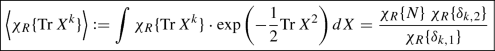 (8)
(8)where X is an \(N\times N\) matrix, and the generating function of all correlators is
$$\begin{aligned}&\int \exp \left( -{1\over 2}\mathrm{Tr}\,X^2+\sum _k{p_k\over k}\ \mathrm{Tr}\,X^k\right) dX \nonumber \\&\quad = \sum _R{ \chi \{p_k\} \chi _R\{N\}\ \chi _R\{\delta _{k,2}\}\over \chi _R\{\delta _{k,1}\}} \end{aligned}$$(9) -
Trigonometric (unitary type) matrix model
This model is given by the eigenvalue integral, and the correlators are [21]
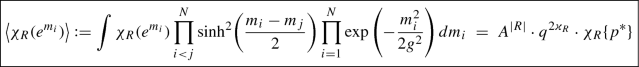 (10)
(10)When averaging, the argument of character in the integrand is the diagonal matrix with the entries \(e^{m_i}\), and, at the r.h.s., the parameters are \(q = e^{g^2/2}\), \(A=q^N=e^{Ng^2/2}\), the exponent \(\varkappa _R = \sum _{(x,y)\in R}(y-x)\), and the time variables \(p^*_k = \frac{A^{k}-A^{-k}}{q^k-q^{-k}}\) in the argument of the character at the r.h.s. lie in the “topological locus” obtained by the q-deformation of \(p_k = N\) in (8).
-
Knot matrix model
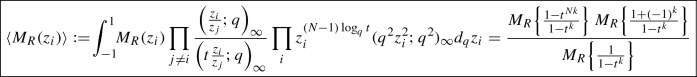
Further deformation of the measure to the knot eigenvalue model gives basically the same expression for the correlators [22, 23]:
 (11)
(11)with \(q=e^{\frac{g^2}{2ab}}\).
The correlators of \(\left\langle \chi _R(e^{m_i}) \right\rangle \) are more involved this time, but are related to the HOMFLY-PT polynomials of the torus knots \({{\mathcal {H}}}_R^{\mathrm{Torus}_{a,b}}(A,q)\) q1 [22, 23]:
$$\begin{aligned} \left\langle \chi _R(e^{m_i}) \right\rangle = {{\mathcal {H}}}_R^{\mathrm{Torus}_{a,b}}(A,q) = \chi _R\{N\} \cdot H_R^{\mathrm{Torus}_{a,b}}(A,q)\nonumber \\ \end{aligned}$$(12)where
$$\begin{aligned} {{\mathcal {H}}}_R^{\mathrm{Torus}_{a,b}}(A,q)&= \left\langle \sum _{Q\vdash a|R|} c_{R,Q} \chi _Q(e^{m_i\over a}) \right\rangle \nonumber \\&= A^{\frac{b|R|}{a}}\sum _{Q\vdash a|R|} c_{R,Q} \cdot q^{\frac{2b \varkappa _Q}{a} } \cdot \chi _Q\{p^*\}\nonumber \\ \end{aligned}$$(13)where \(c_{R,Q}\) are peculiar Adams coefficients [24, 25].
Generalization to non-torus knots, for example, like that in [26, 27], remains to be analyzed.
-
q, t deformed Gaussian Hermitian model
The eigenvalue q, t-deformed Gaussian Hermitian model is associated with a deformation of Schur polynomials: all of them in the formula (8) are replaced by the corresponding Macdonald polynomials \(M_R\) [28]:
 (14)
(14)where
$$\begin{aligned} (z;q)_\infty :=\prod _{k=0}^{\infty }(1-q^kz) \end{aligned}$$(15)and the integral is defined to be the Jackson integral,
$$\begin{aligned} \int _{-1}^1 d_qz f(z):=(1-q)\sum _{k=0}^\infty q^k\Big (f(\xi q^k)+f(-\xi q^k)\Big ) \end{aligned}$$(16)The measure \(d\mu _{q,t}(z)=(q^2z^2;q^2)_\infty d_qz\) gives rise to the Gaussian measure \(d\mu _G(z)=\exp \Big (-{1\over 2}z^2\Big )dz\) in the limit of \(q\rightarrow 1\).
One can expect also a further extension of similar character identities to the elliptic q, t model [29, 30].
-
Monomial non-Gaussian models
Superintegrability is in no way restricted to the Gaussian integration measures or their deformations, though beyond them the knowledge is still restricted. The most important example is provided by monomial non-Gaussian actions:
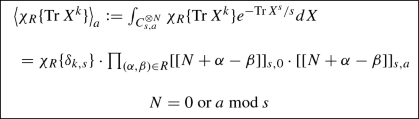 (17)
(17)where we used the notation from (4). The new trick here is the use of a special star-like (closed) integration contour \(C_{s,a}\):
$$\begin{aligned}&\int _{C_{s,a}} F(x)\ e^{-x^s/s} \,dx \,=\ \sum _{b=1}^s e^{-2\pi i(a-1)b/s} \nonumber \\&\quad \cdot \int _0^\infty F\big (e^{2\pi ib/s}x\big )\ e^{-x^s/s}\, dx \end{aligned}$$(18)which picks up only the powers of x, which are equal to \(a-1\, \mathrm{mod}\, s\), in particular,
$$\begin{aligned} \int _{C_{s,a}} x^ke^{-x^s/s} dx=\delta _{k+1-a}^{(s)}\cdot \Gamma \left( {k+1\over s}\right) \end{aligned}$$(19)\(\delta _k^{(s)}\) is defined to be 1 if \(k=0\) mod s and to vanish otherwise. This makes the answer depending on an additional parameter \(a=0,\ldots s-1\). The r.h.s. of (17) contains some factors \(N+j\) from \(\chi _R\{N\}\), (5), that is, those with \(N+i = 0,a\, \mathrm{mod}(s)\), and, hence, its vanishing depends also on the value of N. Note that if the condition \(N=0\ \hbox {or}\ a\ \hbox {mod}\ s\) is not satisfied, one can not define the correlator by the condition \(\langle 1\rangle =1\) because of zeroes in the denominator. Note also that the Vandermonde determinant in the integrand is independent of s and a. For more details, see the original paper [31].


In this paper, we extend these results to the simplest background field models: the matrix integral over \(N_1\times N_2\) complex matrices X with the measure
where \(N_1\times N_1\) matrix A and \(N_2\times N_2\) matrix B are fixed external matrices, and the Hermitian generalized Kontsevich model [32, 33] in background matrix field \(\Lambda \), i.e. the matrix integral over \(N\times N\) Hermitian matrix X with the measure
and \(\Lambda \) is an external \(N\times N\) matrix. In this paper, we consider these two examples, the potential in the second one being \(W(X) = -\frac{X^3}{3}\), which is just the original Kontsevich model [34]. Remarkably, the difference between these two models is severely increased in this case: in particular, in the Hermitian case, only one background field can be easily handled.
The question we address is what are the functions of X-variables that have simple and explicitly calculable averages. As we demonstrate in this paper, in the complex case, these are still the Schur polynomials \(\chi _R\{\mathrm{tr}\,(X{\bar{X}})^k\}\), however, the r.h.s. of (1) now contains traces of A and B instead of \(N_1\) and \(N_2\):

see Sect. 2 below for details, and for generalization to the complex tensor model. In the Hermitian (Kontsevich) case, the story makes a new twist: the relevant functions are more restricted Q Schur polynomials, see Sect. 3.3 for the correlators in this case,

and Sect. 4.2 for the combinatorial expression for the Kontsevich model

Contributing here are only diagrams R with all lines of even length. Equation (24) can be considered as the main new result of this paper. Important feature of formulas (22)–(24) is that they depend on the matrix size only implicitly, through the traces of powers of background fields. This is the crucial feature, which allows one to forget about the matrix-integral origin/realization of these models, in particular to treat them in terms of \(\tau \)-functions of integrable hierarchies [32, 33].
2 Rectangular complex model
2.1 Correlators in terms of permutations
We start with calculating the correlators in the complex matrix model with the external matrix (see [35] for a square matrix example), and use the symmetry group technique worked out in [8]. In this section, we closely follow that paper.
We consider the rectangular complex model
with correlators defined as
where X is \(N_1\times N_2\) rectangular matrix, A and B are square matrices of sizes \(N_1\times N_1\) and \(N_2\times N_2\) respectively, and (notice that, with this definition, the matrix multiplication is defined by convolution of the first indices with each other, and of the second indices with each other)
The pair correlator is equal to
The 2m-point correlator can be labelled by a permutation of indices \(\sigma \) that belongs to the symmetric group \(S_m\):
In order to calculate this correlator, we apply the Wick theorem and use formula (28):
and obtain
where
and \(l_\gamma \) is the number of cycles in the permutation \(\gamma \), with \(i(\gamma )\) denoting the i-th cycle in the permutation \(\gamma \).
Now we use the standard identity [19]
Here the sum goes over all Young diagrams R with \(|{\gamma }|\) boxes, \(\chi _R\{p\}\) is the Schur polynomial (the character of the linear group GL(N)), \(p_{\gamma }=\prod _{i=1}^{l_\gamma }p_{\gamma _i}\) and \(\psi _R({\gamma })\) is the character of the symmetric group \(S_{|R|}\). Now using the orthogonality relation
where \(d_R:=\chi _R\{\delta _{k,1}\}\), we finally come to
where the sizes of R and \(\sigma \) coincide.
2.2 Complex model in background fields
Let us now use the Frobenius formula [19]
where \(|\gamma |\) is the size of the Young diagram R, and the orthogonality relation (34) with the particular value \(\psi _R(id)=\psi _R([1^{|R|}])=|R|!d_R\). Then, one immediately obtains from (35)

This generalizes the answer (1) to the case of \(A\ne I\), \(B\ne I\).
Similarly to (7), we also can obtain the combinatorial expression for the generating function

2.3 Tensor model in background fields
The results of this section for the complex matrix model can be straightforwardly extended to the Gaussian tensor model in background fields. To this end, we follow [36, 37] and again apply the technique of [8].
The Gaussian tensor model is a model of complex r-tensors \(X_{a^1,...a^r}\) where each subscript runs through its interval \(a_i=1,\ldots ,N_i\), in the background of r external square matrices \(A_{(i)}\) of the sizes \(N_i\) with the Gaussian action
Gauge invariant operators at the level m in any (not obligatory Gaussian) tensor model are the tensorial counterparts of “multi-trace” operators
labeled by the set of m elements \(\sigma _i\) of the permutation group \(S_m\). In fact, the labeling is reduced to a double coset \(S_m\backslash S_m^{\otimes r}/ S_m\) [38,39,40,41,42], but we do not need these details here.
There is also a distinguished set of operators called generalized characters in [36, 37] that are defined as
These generalized characters do not form a full basis in the space of all gauge invariant operators, instead they form an over-complete basis in the space of all gauge invariant operators with non-vanishing Gaussian averages [36, 37].
The pair correlator is now \( \left\langle X_{a^1_p,...a^r_p}{\bar{X}}^{b^1_p,...b^r_p}\right\rangle =\left( A_{(1)}^{-1}\right) _{a_1}^{b_1}\cdots \left( A_{(r)}^{-1}\right) _{a_r}^{b_r} \) and, in complete analogy with what we were doing in the complex matrix model case, we obtain the averages of these generalized characters

where
and \(z_\Delta :=\prod _k k^{m_k}m_k!\) is the standard symmetric factor of the Young diagram (order of the automorphism). In the case of \(r=3\), \(C_{R_1,R_2,R_3}\) are the Clebsch-Gordan coefficients of the three irreducible representations \(R_1\), \(R_2\), \(R_3\) of the symmetric group.
3 Correlators in Hermitian model
3.1 Examples of correlators
Let us calculate the correlators in the Gaussian Hermitian matrix model with external fields
Since the matrices are square, we return to the standard convention of convolution of indices in the matrix multiplication. One could expect that, similarly to coming from the rectangular complex model to the Gaussian Hermitian one, the results will not be too much different from those in Sect. 2. It turns out, however, not to be the case, and both the calculations in the Hermitian case with the external field are much more tedious even in the case of one external matrix, and the results remarkably differ from those of Sect. 2. We consider here only the case of one external matrix, i.e. the correlators of the form
Since, the partition function is an invariant function of the external matrix \(\Lambda \), i.e. depends only on its traces, it suffices to choose \(\Lambda \) diagonal. Similarly to (32), we define \(p_k:=\mathrm{Tr}\,\Lambda ^{-k}\).
In this model, the pair correlator in terms of eigenvalues \(\lambda _i\) of the (diagonal) matrix \(\Lambda \) is equal to
Here is the difference with the case of two external matrices: in that case one can not work in terms of eigenvalues, and the pair correlator is much more involved.
Now we consider examples of simple correlators in order to demonstrate the structure of answers.
First consider \(\langle \mathrm{Tr}\,X^3\cdot \mathrm{Tr}\,X^3\rangle =\langle X_{ij}X_{jk}X_{ki}X_{\alpha \beta }X_{\beta \gamma }X_{\gamma \alpha }\rangle \). This average is equal to the sum of products of pairings: \(\langle X_{ij}X_{jk}\rangle \langle X_{ki}X_{\alpha \beta }\rangle \langle X_{\beta \gamma }X_{\gamma \alpha }\rangle \) plus all possible other pairings. Totally, there are 15 different possibilities: 3 terms of the form
three terms of the form
and nine terms of the form
Note that \(C_2+3C_3=p_1^3/2\). Thus, we finally obtain \(\langle \mathrm{Tr}\,X^3\cdot \mathrm{Tr}\,X^3\rangle =3p_3+12p_1^3\).
Consider examples of all correlators up to the level 6 (for the sake of brevity, we use the notation \(\xi _k:=\sum _{i,j}{1\over (\lambda _i+\lambda _j)^k}\)):


and all odd level correlators evidently vanish.
These examples demonstrate that the correlators that involve traces of only odd degrees of the matrix X (they are boxed in (49)) are expressed only through the times (32), moreover, through the odd times. We will return to other correlators elsewhere, and here we consider only this type of correlators. We will need a set of polynomials of odd times that gives a complete basis and forms a closed ring.
3.2 Q Schur polynomials
Emergence of only the odd times immediately gives one a hint to use the Q Schur polynomials instead of the standard Schur polynomials, as we did in the previous sections. These polynomialsFootnote 1 depend only on odd time-variables \(p_{2k+1}\) and only on strict Young diagrams \(R=\{r_1>r_2>\cdots>r_{l_R}>0\}\in \hbox {SP}\). They were introduced by I. Schur [44] in the study of projective representations of symmetric groups, and were later identified by I. Macdonald [45] with the Hall-Littlewood polynomials \(\hbox {HL}_R\{p\}:=\hbox {Mac}_R\{p\}\Big |_{q=0}\) at \(t=-1\):
Macdonald’s observations were that \(\hbox {HL}_R\{p\}\) for \(R\in \hbox {SP}\) depend only on odd time-variables \(p_{2k+1}\), and that \(\hbox {HL}_R\{p\}\) for \(R\in \hbox {SP}\) form a sub-ring, i.e. the Littlewood-Richardson coefficients \({{\mathcal {N}}}_{R_1,R_2}^R\) in the ring
vanish for \(R\notin \hbox {SP}\), provided \(t=-1\) and \(R_1,R_2\in \hbox {SP}\). Note that \(\hbox {HL}_R\{p\}\) do not vanish for \(R\notin \hbox {SP}\), and then they can also depend on even \(p_{2k}\), thus the set of \(Q_R\{p\}\) is not the same as the set of \(\hbox {HL}_R\), it is a sub-set, and a sub-ring.
There is also a manifest way to construct the Q Schur polynomial as a Pfaffian (see, e.g., [43, Eq. (74)]).
The Q Schur polynomials form a system, which has very close properties to the standard Schur functions, only they form a basis in a subspace of time-variables. In particular, there is a counterpart of the Frobenius formula (36), for the Q Schur polynomials it states

where OP (odd partitions) is a set of Young diagrams with all lengths of lines odd, and \(\Psi _R(\Delta )\) are the characters of the Sergeev group [46, 48]. As any characters, they satisfy the orthogonality conditions:

Actually relevant for the Q Schur polynomials is the restriction to odd times, i.e. the Young diagram \(\Delta \) in (52), which defines the monomial \(p_\Delta = \prod _{i}^{l_\Delta } p_{\Delta _i}\) should have all the lines of odd length: \(\Delta \in \hbox {OP}\). Therefore of crucial importance is the celebrated one-to-one correspondence between the sets of \(\hbox {SP}\) and \(\hbox {OP}\).
At last, the Q Schur polynomials satisfy the Cauchy formula, which we write in a form similar to (6), because this is how it will be used in Sect. 4.2 below:

3.3 Combinatorial expression for correlators
We are now ready to formulate a nice result for the correlators (44) in terms of the Q Schur polynomials. Let us denote through 2R the Young diagram produced from the diagram R by doubling all line lengths, and denote through R|2 the Young diagram with all even line lengths (in this case, R/2 denotes the Young diagram with all line lengths being half of those of R)Footnote 2. Then (compare with [49]),

For the quantity \(Q_{R}\{\delta _{k,1}\}\), there is a counterpart of the standard hook formula (2):
It is non-zero only for \(R\in \hbox {SP}\), and
Note that, unlike most formulas in the Introduction, the r.h.s. in (55) is sensitive to relative normalization of two different Q-Schur functions \(Q_R\) and \(Q_{R/2}\), which is actually well defined, because these quantities are characters of a group and they form an algebra with integer Littlewood-Richardson coefficients. Another property that distinguishes this normalization is that, with the scalar product
the Q-polynomials are orthonormal:
and the Cauchy formula (54) acquires an especially simple form with unit coefficients in the sum.
4 Kontsevich model
Now we are ready to consider the Kontsevich model given by the integral [34]
and it can be further generalized to non-cubic potentials [32, 33], including the quadratic one, when the model is equivalent to the Hermitian matrix model [3]. In this paper, we concentrate on the original cubic case, and we denote the background field by \(\Lambda ^2\) to simplify the formulas in Sect. 4.2.
4.1 Kontsevich model in the character phase
The normalization of measure of the Kontsevich integral depends on the phase of the model [50]. In the character phase, the integral is understood as a formal series in positive powers of \(\mathrm{Tr}\,\Lambda ^k\), and the generating function of the correlators is defined to be
Since the cubic part does not depend on the angular part of the matrix X, one can first perform the angular integration using the expansion [51] of the Itzykson-Zuber integral [52, 53]
so that one remains with
and then calculate the correlators \(\left\langle \chi _R\{\mathrm{Tr}\,X^k\}\right\rangle \) for the star-like integration contours directly applying formulas like (17). Thus, in this phase, the expression in terms of characters is straightforward and nearly obvious.
4.2 Kontsevich model in the Kontsevich phase
Much more interesting is the case of Kontsevich phase, where the character calculus is much less trivial. In this phase, the model is given by the integral
and is understood as a formal series in \(\mathrm{Tr}\,\Lambda ^{-k}\). The simplest way to deal with this integral is to shift the integration variable to the saddle point \(X\rightarrow X+\Lambda \) so that the integral takes the form
and one calculates this integral perturbatively using the Cauchy formula (54),
Since, for even sizes of Young diagrams |R|, \(Q_R\{-p_k\}=Q_R\{p_k\}\) and averages are non-vanishing only for even sizes, one finally obtains the Kontsevich partition function:

where we used (55) for the average. Note that, because of the factor \(Q_{2R}\{\delta _{k,3}\}\), this sum effectively runs over R of sizes divisible by 3.
As expected in Kontsevich phase, this partition function depends on the matrix size N only through the variables \(\mathrm{Tr}\,\Lambda ^{-k}\). This is exactly the same phenomenon which we observed in (22).
Derivation of the formula (67) could be one of the goals in [49], but at that time the Q Schur polynomials were even less known then now, and an explicit answer like this was unavailable.
4.3 Integrability and character expansion
Note that expansion of the partition function in characters typically allows one to check if it is a \(\tau \)-function of the KP hierarchy immediately by checking that the expansion coefficients satisfy the Plücker relations. For instance, this is the case for the partition functions (7) and (9). Indeed, any partition function of the form
with the function \(w_R\) being the product
and \({\bar{p}}_k\) just arbitrary parameters, is a KP \(\tau \)-function [11, 54,55,56], since arbitrary Schur polynomial \(S_R\{{\bar{p}}\}\) satisfies the Plücker relations, and multiplying any solution to the Plücker relations by \(w_R\) of the form (69) preserves the solution. Now using (5) and fixing \({\bar{p}}_k=N_2\), one obtains that (7) is of the form (68). Similarly, fixing \(p_k=\delta _{k,1}\), one obtains that (9) is of the form (68).
As we explained in [43, Sect. 8] (see also [57,58,59,60]), similarly looking at expansion in the Q Schur polynomials, one can expect that the partition function is a \(\tau \)-function of the BKP hierarchy. Moreover, we proposed an example of expansion literally repeating formula (7) but with the Schur polynomials substituted by the Q Schur polynomials, though have not managed to construct a matrix model that possesses such an expansion. Hence, it is surprising to realize that the Kontsevich model, which is a \(\tau \)-function of the KP hierarchy [32, 33], not BKP have a similar character expansion in the Q Schur polynomials. This realization in terms of matrix model is especially important as the Q Schur polynomials are related to the spin Hurwitz numbers and to the corresponding cut-and-join operators [43].
Let us emphasize that, as soon as the Kontsevich partition function is a KdV \(\tau \)-function [32, 33], and the KdV \(\tau \)-function depends on odd times only, this is quite natural to expand the Kontsevich partition function in the Q Schur polynomials, which, in variance with the ordinary Schur polynomials, depends only on odd times. One may ask why people usually consider expansions of KdV \(\tau \)-functions into the ordinary Schur polynomials and not into the Q Schur polynomials (see, however, [61]), which could look more natural. The reason is that the standard technique of the KdV hierarchy as an embedding into the KP hierarchy uses the formalism of free fermions [62], hence the ordinary Schur polynomials, and it is only using the neutral fermions that gives rise to the Q Schur polynomials, but this type of fermions is associated with the BKP hierarchy [57,58,59,60, 63, 64]. We will consider this issue in detail elsewhere.
5 Conclusion
In this paper, we extended the superintegrability relation \(\langle character\rangle \sim \mathrm{character}\) to the second kind of matrix models, depending on background fields. This provides a very nice generalization for the complex matrix model, where dimensions of matrices are lifted to more general traces of background matrices. The best known example of the background-field model is, however, different: this is the Kontsevich model, which is rather analogous to the Hermitian, not complex model. In the Hermitian case, the simple formulas are known to get a little more involved: they include characters at a peculiar locus \(\delta _{k,s}\), where s is the power of the potential. Thus, it was an intriguing question what happens in background fields. Our result in this paper is for the ordinary Kontsevich model with cubic potential, and it is that the very set of characters is changed from the Schur polynomials to the very interesting set of Q Schur polynomials, and then their averages are given by a rather transparent formula (55). The formula is, however, somewhat non-trivial, because it requires a correlation between normalization of different Q Schur polynomials, in most other examples this does not matter because just a single character appears in the answer which is made from its values at three different loci. In the Kontsevich case, this is different, and this adds new colors to the yet-no-so-well-known subject of Q Schur polynomials.
It is important that the superintegrability-related expansion (67) of the Kontsevich partition function in Q Schur polynomials is much simpler than the expansion through the ordinary Schur polynomials, which could seem natural from the point of view of KP integrability [4,5,6, 65]. Indeed, the coefficients of the latter expansion were found in [66, 67] and turned out to be quite complicated and do not expose any clear structure. Even the character nature of the coefficients is not evident in this KP induced expansion. Equation (67) is obviously free from all such drawbacks, in full accordance with the expectations. It, however, remains a problem to lift (67) to generalized Kontsevich model [32, 33], while the ordinary Schur expansion of them should be a direct lifting of [66, 67].
Data Availability Statement
This manuscript has no associated data or the data will not be deposited. [Authors’ comment: This is a theoretical study, and no experimental data has been listed.]
Notes
More detailed review of these polynomials can be found, e.g., in [43].
For instance, an example of R|2 is \(R=[6,4,2]\). In this case, \(R/2=[3,2,1]\) and \(2R=[12,8,4]\).
References
A. Gerasimov, A. Marshakov, A. Mironov, A. Morozov, A. Orlov, Nucl. Phys. B 357, 565–618 (1991)
S. Kharchev, A. Marshakov, A. Mironov, A. Orlov, A. Zabrodin, Nucl. Phys. B 366, 569–601 (1991)
S. Kharchev, A. Marshakov, A. Mironov, A. Morozov, Nucl. Phys. B 397, 339–378 (1993). arXiv:hep-th/9203043
A. Morozov, Phys.Usp.(UFN) 37 (1994) 1; arXiv:hep-th/9502091; arXiv:hep-th/0502010
A. Mironov, Int. J. Mod. Phys. A 9, 4355 (1994)
A. Mironov, Phys. Part. Nucl. 33, 537 (2002). arXiv:hep-th/9409190
A. Mironov, A. Morozov, Phys. Lett. B 771, 503 (2017). arXiv:1705.00976
A. Mironov, A. Morozov, Phys. Lett. B 774, 210 (2017). arXiv:1706.03667
A. Mishchenko, A. Fomenko, Funct. Anal. Appl. 12, 113 (1978)
W. Miller Jr., S. Post, P. Winternitz, J. Phys. A46, 423001 (2013). arXiv:1309.2694
A. Alexandrov, A. Mironov, A. Morozov, S. Natanzon, JHEP 11, 080 (2014). arXiv:1405.1395
H. Itoyama, A. Mironov, A. Morozov, JHEP 1706, 115 (2017). arXiv:1704.08648
C. Kristjansen, J. Plefka, G.W. Semenoff, M. Staudacher, Nucl. Phys. B 643, 3–30 (2002). arXiv:hep-th/0205033
S. Corley, A. Jevicki, S. Ramgoolam, Adv. Theor. Math. Phys. 5, 809–839 (2002). arXiv:hep-th/0111222
J. Harer, D. Zagier, Invent. Math. 85, 457–485 (1986)
C. Itzykson, J.-B. Zuber, Comm. Math. Phys. 134, 197–208 (1990)
S.K. Lando, A.K. Zvonkin, Embedded graphs, Max-Plank-Institut für Mathematik, Preprint 2001 (63)
A. Morozov, S. Shakirov, JHEP 0904, 064 (2009). arXiv:0902.2627
W. Fulton, Young tableaux: with applications to representation theory and geometry, LMS (1997)
R. de Mello Koch, S. Ramgoolam, arXiv:1002.1634
A. Mironov, A. Morozov, JHEP 1808, 163 (2018). arXiv:1807.02409
M. Tierz, Mod. Phys. Lett. A 19, 1365–1378 (2004). arXiv:hep-th/0212128
A. Brini, B. Eynard, M. Mariño, Annales Henri Poincaré. Vol. 13. No. 8. SP Birkhäuser Verlag Basel (2012). arXiv:1105.2012
M. Rosso, V.F.R. Jones, J. Knot Theory Ramifications 2, 97–112 (1993)
X.-S. Lin, H. Zheng, Trans. Am. Math. Soc. 362, 1–18 (2010). arXiv:math/0601267
A. Alexandrov, A. Mironov, A. Morozov, An. Morozov, JETP Lett. 100, 271–278 (2014) (Pis’ma v ZhETF 100 (2014) 297–304). arXiv:1407.3754
A. Alexandrov, D. Melnikov, JETP Lett. 101, 51–56 (2015). arXiv:1411.5698
A. Morozov, A. Popolitov, S. Shakirov, Phys. Lett. B 784, 342 (2018). arXiv:1803.11401
A. Mironov, A. Morozov. arXiv:2011.02855
A. Mironov, A. Morozov. arXiv:2011.01762
C. Cordova, B. Heidenreich, A. Popolitov, S. Shakirov, Commun. Math. Phys. 361, 1235 (2018). arXiv:1611.03142
S. Kharchev, A. Marshakov, A. Mironov, A. Morozov, A. Zabrodin, Phys. Lett. B 275, 311 (1992). arXiv:hep-th/9111037
S. Kharchev, A. Marshakov, A. Mironov, A. Morozov, A. Zabrodin, Nucl. Phys. B 380, 181 (1992). arXiv:hep-th/9201013
M. Kontsevich, Commun. Math. Phys. 147, 1 (1992)
E. Langmann, R.J. Szabo, K. Zarembo, JHEP 01, 017 (2004). arXiv:hep-th/0308043
H. Itoyama, A. Mironov, A. Morozov, JHEP 1912, 127 (2019). arXiv:1909.06921
H. Itoyama, A. Mironov, A. Morozov, Phys. Lett. B 802, 135237 (2020). arXiv:1910.03261
J. Ben Geloun, S. Ramgoolam, arXiv:1307.6490
R. de Mello Koch, D. Gossman, L. Tribelhorn, JHEP 2017, 011 (2017). arXiv:1707.01455
P. Diaz, S.J. Rey,. arXiv:1706.02667
J. Ben Geloun, S. Ramgoolam, arXiv:1708.03524
H. Itoyama, A. Mironov, A. Morozov, Nucl. Phys. B 932, 52 (2018). arXiv:1710.10027
A. Mironov, A. Morozov, S. Natanzon, Eur. Phys. J. C 80, 97 (2020). arXiv:1904.11458
I. Schur, J. Reine Angew. Math. 139, 155–250 (1911)
I.G. Macdonald, Symmetric functions and Hall polynomials, 2nd edn. (Oxford University Press, Oxford, 1995)
A. Sergeev, Math. Sb. USSR 51, 419–427 (1985)
M. Yamaguchi, J. Algebra 222, 301–327 (1999). arXiv:math/9811090
A. Kleshchev, Linear and projective representations of symmetric groups, Cambridge Tracts in Mathematics 163 (Cambridge Univ. Press, Cambridge, 2005)
P. Di Francesco, C. Itzykson, J.B. Zuber, Commun. Math. Phys. 151, 193 (1993). arXiv:hep-th/9206090
A. Mironov, A. Morozov, G.W. Semenoff, Int. J. Mod. Phys. A 11, 5031 (1996). arXiv:hep-th/9404005
A. Y. Morozov, Theor. Math. Phys. 162 (2010) 1 [Teor. Mat. Fiz. 161 (2010) 3]. arXiv:0906.3518
Am Harish-Chandra, J. Math. 79, 87 (1957)
C. Itzykson, J.B. Zuber, J. Math. Phys. 21, 411 (1980)
S. Kharchev, A. Marshakov, A. Mironov, A. Morozov, Int. J. Mod. Phys. A 10, 2015 (1995). arXiv:hep-th/9312210
A. Orlov, D.M. Shcherbin, Theor. Math. Phys. 128, 906–926 (2001)
A. Orlov, Theor. Math. Phys. 146, 183–206 (2006)
A. Orlov, Theor. Math. Phys. 137, 1574–1589 (2003). math-ph/0302011
J. Harnad, J.W. van de Leur, AYu. Orlov, Theor. Math. Phys. 168, 951–962 (2011). arXiv:1101.4216
J.W. van de Leur, A.Yu. Orlov, arXiv:1404.6076. arXiv:1611.04577
A. Yu. Orlov, T. Shiota, K. Takasaki. arXiv:1201.4518. arXiv:1611.02244
J.J.C. Nimmo, A. Orlov, Glasgow Math. J. 47 (A), 149–168. arXiv:nlin/0405009 (2005)
E. Date, M. Jimbo, M. Kashiwara, T. Miwa, R.I.M.S. Symp, Non-linear integrable systems: classical theory and quantum theory (World Scientific, Singapore, 1983)
E. Date, M. Jimbo, M. Kashiwara, T. Miwa, Phys. D 4, 343–365 (1982)
M. Jimbo, T. Miwa, Publ. RIMS Kyoto Univ. 19, 943–1001 (1983)
Y. Ohta, J. Satsuma, D. Takahashi, T. Tokihiro, Prog. Theor. Phys. Suppl. 94, 210 (1988)
J. Zhou. arXiv:1306.5429
F. Balogh, D. Yang, Lett. Math. Phys. 107, 1837 (2017). arXiv:1412.4419
Acknowledgements
This work was supported by the Russian Science Foundation (Grant No.20-12-00195).
Author information
Authors and Affiliations
Corresponding author
Rights and permissions
Open Access This article is licensed under a Creative Commons Attribution 4.0 International License, which permits use, sharing, adaptation, distribution and reproduction in any medium or format, as long as you give appropriate credit to the original author(s) and the source, provide a link to the Creative Commons licence, and indicate if changes were made. The images or other third party material in this article are included in the article’s Creative Commons licence, unless indicated otherwise in a credit line to the material. If material is not included in the article’s Creative Commons licence and your intended use is not permitted by statutory regulation or exceeds the permitted use, you will need to obtain permission directly from the copyright holder. To view a copy of this licence, visit http://creativecommons.org/licenses/by/4.0/.
Funded by SCOAP3
About this article

Cite this article
Mironov, A., Morozov, A. Superintegrability of Kontsevich matrix model. Eur. Phys. J. C 81, 270 (2021). https://doi.org/10.1140/epjc/s10052-021-09030-x
Received:
Accepted:
Published:
DOI: https://doi.org/10.1140/epjc/s10052-021-09030-x