
Abstract
We present our first attempt to develop a model for soft interactions at high energy, based on the BFKL Pomeron and the CGC/saturation approach. We construct an eikonal-type model, whose opacity is determined by the exchange of the dressed BFKL Pomeron. The Green function of the Pomeron is calculated in the framework of the CGC/saturation approach. Using five parameters we achieve a reasonable description of the experimental data at high energies (\(W\ge 0.546\) TeV) with overall \(\chi ^2/d.o.f. \approx 2\). The model results in different behavior for the single- and double-diffraction cross sections at high energies. The single-diffraction cross section reaches a saturated value (about 10 mb) at high energies, while the double-diffraction cross section continues growing slowly.
1 Introduction
The strong interaction at high energies is one of the most difficult and unrewarding problems of high energy physics. The reason for this is the embryonic stage of our understanding of non-perturbative QCD. Traditionally, we consider the strong interaction at high energy as a typical example of processes that occur at long distances, where the unknown force confining quarks and gluons plays a crucial role, making all our theoretical efforts to treat these processes fruitless. The description of these processes which we need for practical purposes is the field of high energy phenomenology, based on Pomeron calculus [1–4]. The LHC data [5–10] shows that in many cases models based on this phenomenology failed to agree with the results of the classical set of soft interaction data: total, elastic, and diffraction cross section as well as elastic slope and the inclusive production of the secondary hadrons [11–18]. However, there is a glimpse of hope due to the following two facts: models that fit the LHC data have been proposed [19–21]; and after two decades of experience in high energy phenomenology we have learned that the more theoretically based the phenomenological input is, the more appropriate and apprehensible, the resulting description of the data we obtain.
In Ref. [22] we reviewed our model which describes successfully all high energy data, including those at the LHC, and which incorporates theoretical ingredients from N = 4 SYM [23–30] and from perturbative QCD [31–39]. In the present paper we improve this approach, by including more pertinent theoretical input. First, we introduce a more constructive meaning to our old idea [15, 40] that there is only one Pomeron that describes both soft and hard interactions. In perturbative QCD the BFKL Pomeron at high energy takes the following form [31, 32]:Footnote 1

 denotes the BFKL Pomeron Green function, \(\bar{\alpha }_S\) the QCD coupling, \(r\) and \(R\) are the sizes of the two interacting dipoles. \(Y =\ln s\), where \(s = W^2\). \(W\) denotes the energy of the interaction, and \(b\) the impact parameter for the scattering amplitude of the two dipoles.
From Eq. (1.1) it is obvious that the BFKL Pomeron is not a pole in angular momentum but a branch cut, since its Y-dependence has an additional \(\ln s\) term; it does not reproduce the exponential decrease at large \(b\), which follows from the general properties of analyticity and unitarity [41, 42]; as the exchange of the BFKL Pomeron depends on the sizes of the dipoles, consequently, the BFKL Pomeron does not factorize.
The Pomeron that appears in N \(=\) 4 SYM [23–25] corresponds to the BFKL Pomeron in QCD with the following glossary:

where \(\lambda = 4 \pi N_c \alpha ^{YM}_S\) and \(\alpha ^{YM}_S \) denotes the QCD-like coupling.
Hereby we generalize our approach, dealing with the BFKL Pomeron instead of the simple Regge pole that was used in our previous model.
The second innovation is related to the Pomeron interaction. The LHC data supports the assumption that dense systems of partons (gluons) are produced in the proton–proton interactions at high energy. Such a system of partons appears naturally in the CGC/saturation approach [47–66], and it provides a successful description of the general properties of the average event at the LHC [67–71], and of the long range rapidity angular correlations [72–74]. In this paper, we use the CGC/saturation approach to describe the Pomeron interactions, replacing the Pomeron calculus. This strategy allows us not only to treat the Pomeron interactions, but also to include the saturation phenomenon, which was beyond the scope of our previous model.
2 Model: theoretical ingredients
2.1 Parton cascade of one dipole in the saturation region
The parton cascade, which originates from the decay of one gluon to two gluons in QCD, can be described equally well in two ways. The first, using the QCD expression for this decay, describes the change of probability to have \(n\) gluons at rapidity \(Y\), due to the decay of one gluon to two. The equation in this approach is a linear functional equation for the generating functional (see Refs. [53, 54, 58–65, 75–77]). The alternate way is to sum the Pomeron fan diagrams (see Fig. 1) in the framework of the BFKL Pomeron calculus [78–83].

The structure of the parton cascade for a fast dipole and its relation to the Pomeron interaction. Helical lines denote gluons. The wavy lines describe BFKL Pomerons. The blobs stand for triple Pomeron vertices
In this paper we use the solution of the functional equation which was proposed and discussed in Ref. [84]. For completeness of presentation, we repeat the main ideas of the solution, and explain the physical meaning of the phenomenological parameters that we have introduced in our model.
The first simplification arises when we consider the interaction of the parton cascade with a large target (say with a heavy nucleus). In this case the functional equation reduces to the non-linear Balitsky–Kovchegov equation. The solution of this equation has three distinct kinematic regions.
-
1.
\(r^2 Q^2_s\left( Y, b\right) \ll 1\), where \(Q_s\) denotes the saturation scale [47–52]. The non-linear corrections are small, and the solution is the BFKL Pomeron;
-
2.
\(r^2 Q^2_s\left( Y, b\right) \sim 1\) (vicinity of the saturation scale). The scattering amplitude has the following form [85–87]:
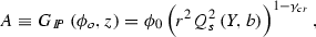 (2.1)
(2.1)where \(\phi _0\) is a constant, and where the critical anomalous dimension \(\gamma _{cr}\) can be found from
$$\begin{aligned} \frac{\chi \left( \gamma _{cr}\right) }{1 - \gamma _{cr}}&= - \frac{\mathrm{d}\chi \left( \gamma _{cr}\right) }{\mathrm{d}\gamma _{cr}} \quad \text{ and }\nonumber \\ \chi \left( \gamma \right)&= 2\psi \left( 1 \right) -\psi \left( \gamma \right) -\psi \left( 1 - \gamma \right) \!. \end{aligned}$$(2.2) -
3.
\(r^2 Q^2_s\left( Y, b\right) \gg 1\) (deeply inside the saturation domain). The amplitude approaches unity [88]:
$$\begin{aligned} A&= 1\!-\!\text{ Const }\exp \Big (\! - \frac{z^2}{2\kappa }\Big ) , \quad \text{ where } \nonumber \\&\quad z\!=\!\ln \left( r^2Q^2_s\left( Y, b\right) \right) =\bar{\alpha }_S\kappa Y+\xi \text{, }\kappa = \frac{\chi \left( \gamma _{cr}\right) }{ 1 - \gamma _{cr}}.\nonumber \\ \end{aligned}$$(2.3)and \( \xi = \ln \left( r^2Q^2_s\left( Y=Y_{0}, b\right) \right) \).

In spite of our understanding of all qualitative features of the solution, we do not have an equation for an analytical solution [66], which we need to reconstruct the parton cascade. The parton cascade can be described as the amplitude for the production of dipoles of size \(r_i\) at impact parameters \(b_i\). This amplitude can be written as

The solution to the non-linear equation is of the following general form:

Comparing Eq. (2.4) with Eq. (2.5) we see
Unfortunately, we cannot find the coefficient \(C_n\), for the general non-linear equation. For the case of the simplified BFKL kernel (see Refs. [84, 88]) the solution can be found, and we can suggest a simple formula that provides a very accurate solution of Eq. (2.5) (see Ref. [84]):

with \(a\) = 0.65.
This formula allows us to find \(\widetilde{C}_n\left( \phi _0, r\right) \), and to reconstruct the amplitude of Eq. (2.4).
2.2 Summing Pomeron loops (MPSI approximation)
It was shown in Ref. [89] that in the BFKL Pomeron calculus for the parton cascade (see Fig. 1), the integration over rapidities of the triple Pomeron vertices, suggests that the value of the typical rapidity is of the order of \(Y - Y_i \sim 1/\Delta _{\text{ BFKL }}\). Consequently, only large Pomeron loops with rapidity of order \(Y\), contribute at high energies [90–93]. To sum such loops we use the MPSI approximation developed in Ref. [90–93]. The essence of this approximation is to use the \(t\)-channel unitarity constraint, which is satisfied by the one BFKL Pomeron exchange. Indeed, at any value of \(Y'\), the BFKL Pomeron has the following property from \(t\)-channel unitarity [47, 94] (see Fig. 2b):

The MPSI approximation is illustrated in Fig. 2a, where the first non-trivial loop diagram is presented. This approximation enables us to evaluate the Pomeron loops, using the fan diagram structure of the parton cascade. The general MPSI equation for the sum of enhanced Pomeron diagrams, has the form which leads to a new Pomeron Green function (dressed Pomeron):

In the last equation we used Eq. (2.6) with
Since, for the proton–proton scattering, \(r = R \), \( z >0\) (see Eq. (2.10)), we are dealing with parton cascades in the saturation domain. We recall that the saturation domain corresponds to \( z>0, ( r^2 Q^2_s \ge 1\)), while \(z < 0 ( r^2Q^2_s \le 1)\) characterizes the perturbative QCD region.

MPSI approximation: the simplest diagram (a) and one Pomeron contribution (b). \(C=\bar{\alpha }_S^2/4 \pi \). \( \vec {x}_1 - \vec {x}_2 = \vec {r}^{'}\). \(\frac{1}{2}(\vec {x}_1 + \vec {x}_2 ) = \vec {b}^{'}\). The wavy lines describe BFKL Pomerons. The blobs stand for triple Pomeron vertices
In Ref. [95–97] the MPSI approximation, as well as the equivalence of the CGC/saturation approach and the BFKL Pomeron calculus, was proven for a wide range of rapidities:
For larger \(Y\) the MPSI approximation does not give the exact answer, since we have not introduced the vertex of the four Pomeron interaction, which violates the simple structure of the parton cascade shown in Fig. 1. The errors that stem from neglecting the four Pomeron interaction, have been evaluated in Ref. [22, 95–97].
3 Model: main formulas and parameters
In this section we describe our model. Its main ingredient is the sum of the Pomeron loops, which leads to a new dressed Pomeron Green function.
3.1 Dressed Pomeron
The resulting Green function of the Pomeron is given by Eq. (2.9). Using Eq. (2.7) and Eq. (2.9) (see Fig. 3a) we obtain the following expression (see Refs. [22, 84] for more details):

where \(\Gamma \left( x \right) \) is the incomplete Euler gamma function (see 8.35 of Ref. [98]). The function \(T\left( Y- Y_0, r, R, b \right) \) can be found from Eq. (2.9) and has the form

where we used two inputs: \(r \!=\! R\) and \(Q^2_s\!=\!\left( 1/(m^2R^2)\right) S\left( b \right) \)
\(\exp \left( \lambda Y\right) \). The parameter \(\lambda =\bar{\alpha }_S\chi \left( \gamma _{cr}\right) /(1 - \gamma _{cr})\) in leading order of perturbative QCD. From phenomenology \(\lambda \) turns out to have the value \(\lambda = 0.2 \div 0.3\) [99, 101, 102]. \(S\left( b\right) \) is a pure phenomenological profile function, which we choose to be of the form
The parameter \(m\) represents the inverse size of the dipole \(m \sim 1/r = 1/R\). Unfortunately, we have no theoretical estimate for this mass. It may be large, reflecting the masses of glueballs and the small size of the typical dipole in a hadron [103]. Note that \(S\left( b\right) \) has a correct, exponential decrease at large \(b\). This is an advantage of our approach, as it enables us to introduce a non-perturbative scale in a physical motivated way, for the observable that characterizes the principal property of the parton cascade. Therefore, in the framework of our approach we do not face the theoretical problem of large \(b\) behavior, which is the main unsolved problem in the CGC/saturation approach [104, 105] (Fig. 3).

The dressed Pomeron in the MPSI approximation (a) and the sum of net diagrams (b). The wavy lines describe BFKL Pomerons. The gray blobs stand for triple Pomeron vertices while the black ones describes the vertex hadron–Pomeron interaction \(g\left( b \right) \)
3.2 Interaction of dressed Pomerons
The interaction of a dressed Pomeron with a hadron is a non-perturbative problem, which cannot be solved for the moment. From the microscopic point of view this interaction depends on the size of a typical dipole in a hadron, on the probability of finding such a dipole, and on the interaction coupling. Since this interaction originates at long distances, we cannot calculate it even in the CGC/saturation approach. Introducing two phenomenological constants, \(g\) and \(m_1\), we describe the vertex of the hadron–Pomeron interaction as follows:
To account for the interaction of the dressed Pomerons with hadrons, we use the strategy that has been suggested in Ref. [14], and which is based on the fact that we anticipate the value of \(g\) in Eq. (3.4) will be large. In this case we can evaluate the scattering amplitude in the following kinematic region of rapidities:

The difference with our previous model reviewed in Ref. [22] lies in the value of  which was a phenomenological parameter, while now we are able to estimate it from the CGC/saturation approach.
Finally, the opacity \(\Omega \) has the form (see Fig. 3b)

where

In Eq. (3.6) we assumed that \(m\gg m_1\). The factor \(1.29\) stem from estimates of the triple Pomeron vertex in the CGC/saturation approach.
3.3 Observables
3.3.1 Elastic amplitude
The elastic amplitude is
3.3.2 Single diffraction
The cross section for single diffraction can be written as
where \( \bar{N}_\mathrm{SD}\left( Y\right) =\int \mathrm{d}^2 b' N_\mathrm{SD}\left( Y, b'\right) \) and \(N_\mathrm{SD}\left( Y, b\right) \) has been calculated in Ref. [84]. It has the form
where \(T = T\left( Y, b \right) \) of Eq. (3.2). This definition of \(T\) is valid only in the region where \(T < 1\). A more general formula is given in Ref. [84]. Equation (3.10) which sums the diagrams of Fig. 4a, where the double wavy lines crossed by the dashed one, denote the dressed Pomeron structure in terms of the produced particle. In Reggeon calculus it is referred to as the cut Pomeron. We would like to emphasis that in our approach this contribution is the solution to the equation for single-diffractive production of Ref. [108], which is given in Ref. [84].

Single (a) and double (b) diffraction production. The double wavy lines describe dressed Pomerons. The double wavy line crossed by the dashed one stands for the dressed Pomeron structure, in terms of produced particles. The blobs stand for the hadron–Pomeron interaction \(g\left( b \right) \) vertices
The profile function for the single-diffraction production is taken from Eq. (3.25) of Ref. [15].
3.3.3 Double diffraction
The double diffraction cross section has the form
\( \bar{N}_\mathrm{DD}\left( Y\right) =\int \mathrm{d}^2 b' N_\mathrm{DD}\left( Y, b'\right) \) and \(N_\mathrm{DD}\left( Y, b\right) \) can be determined from the simple expression

where \(T = T\left( Y, b \right) \) of Eq. (3.2) with the same comments as for Eq. (3.10). Equation (3.11) sums the diagrams shown in Fig. 4b.Footnote 2
The profile \(S_\mathrm{DD}\left( b \right) \) is given by
3.4 Phenomenological parameters
In this section we summarize our phenomenological parameters and provide theoretical estimates for them. Altogether, we have five parameters: \(g\), \(\phi _0\), \(\lambda \), \(m\) and \(m_1\).
-
\(\lambda \) in the CGC/saturation approach, can be calculated in the leading order of perturbative QCD. It characterizes the energy dependence of the saturation scale in proton–proton collisions. Theoretical estimates give \(\lambda = \bar{\alpha }_S\chi \left( \gamma _{cr}\right) /(1 - \gamma _{cr}) \approx 4.88\bar{\alpha }_S\) in leading order of perturbative QCD, where \(\gamma _{cr} = 0.37\). However, the estimates with a running QCD coupling, as well as CGC/saturation phenomenology, lead to \(\lambda = 0.2 \div 0.3\).
-
In the vicinity of the saturation line
 (see Eq. 2.1). \(\phi _0\) denotes the value of the Pomeron Green function on the saturation line (at \(z = 0, r Q_s = 1 \)). The exact value of \(\phi _0\) cannot be determined without specifying the Pomeron–hadron interaction in more detail than we have. However, \(\phi _0 \propto \bar{\alpha }_S^2\) so we expect \(\phi _0\) to be small.
 -
\(m_1\) and \(m\) are pure phenomenological parameters, in our formulas we assumed that \(m \gg m_1\). We make this assumption in order to simplify the formula.
-
\(g\) is a pure phenomenological parameter which we assumed to be larger than
 .
.
 (see Eq.
  .
.4 Fit to the data
4.1 Cross sections and the values of the parameters
We determine the five parameters that our model depends on, by fitting to experimental data for the following set of observables: total, inelastic, and elastic cross sections, for single and double-diffractive production cross sections, and for the slope of the forward elastic differential cross section. We fit to the high energy data with \(W \ge \) 0.546 TeV. We choose the minimal energy \(W = 0.546\) TeV in our fit, as starting from this energy the CGC/saturation approach is able to describe the data on inclusive production in proton–proton collisions (see Ref. [100]). On the other hand the energy \(W = 0.2\) TeV is too low, as at this energy saturation occurs in ion–ion and proton–ion collisions, but not in proton–proton collisions [101].
The quality of the fit can be seen from Fig. 5 and the values of parameters are presented in Table 1.

Comparison with the experimental data: the energy behavior of the total (a), inelastic (b), elastic cross sections (c), as well as the elastic slope (\(B_\mathrm{el}\)) (d), and single diffraction (e) and double diffraction (f) cross sections. The solid lines show our present fit. The data has been taken from Ref. [109] for energies less than the LHC energy. At the LHC energy for total and elastic cross section we use TOTEM data [9, 10] and for single- and double-diffraction cross sections are taken from Ref. [5]
Our first observation is that the values of all parameters are in agreement with our expectations given in Sect. 3.4. Second, the overall fit has \(\chi ^2/d.o.f. \approx 2\) of which 40% is due to our failure to reproduce the TOTEM value of \(B_\mathrm{el}\) at W = 7 TeV, and therefore, except for this point, we have a reasonably good description of the data.
We discuss some regularities in our fit, which could be useful for further and more profound understanding of the microscopic physics.
-
We obtain a good description both of the values and of the energy dependence for total, inelastic, and elastic cross sections in a wide energy range: \(W = 0.546 \div 57\) TeV.
-
At lower energies the values of \(B_\mathrm{el}\) are rather close to the experimental ones, but a glance at Fig. 5d shows that the energy behavior in our model is milder than that of the experimental one. The LHC value of \(B_\mathrm{el}\) is considerably higher than our prediction. A natural conjecture would be that this behavior is a direct consequences of long standing and unsolved problem in the CGC/saturation approach: i.e. the large impact parameter behavior of the BFKL Pomeron [104, 105], however, we do not think that this is correct. Indeed, the problem noticed in Ref. [104, 105] is one of the principal problems of the CGC/saturationapproach, and has not yet been solved. Several theoretical models [106, 107] show that the correct (exponential decreasing \(\exp (-\mu b)\)) large impact parameter behavior of the scattering amplitude, does not influence the BFKL Pomeron, and does not even produce shrinkage of the diffraction peak (i.e. energy behavior of \(B_\mathrm{el}\)). We can also see indications of the weak influence of the large \(b\) tail of the profile function in the data. Indeed, we were able to describe both \(\sigma _\mathrm{tot}\) and \(\sigma _\mathrm{el}\) which could be possible, only if one profile function describes the typical \(b\) behavior correctly. Since there is no reason to expect that large \(b\) behavior could be crucial in the description of the available data, we assume that the CGC/saturation approach will not be changed by the (incorrect) large \(b\) behavior of the BFKL Pomeron, and that all non-perturbative corrections have to be included in \(Q_s\) [87]: the only dimensional parameter of the theory. It should be stressed that this assumption leads to correct exponential fall off of the amplitude in the framework of our approach. We believe that the weak energy dependence of the elastic slope follows mostly from rather small shadowing corrections (see Fig. 6b), which we hope will be alleviated in our future planned two channel treatment.
-
Our single-diffractive production cross section has values within the experimental error, but our model predicts a lower cross section at \(W =\) 7 TeV, than the one given by ALICE [5]. The model’s results are shown in Table 2 and support the idea that the single diffraction is saturated at high energy.Footnote 3 In our model the saturation, and oscillatory behavior, of the single-diffraction cross section stems from two sources: the simple one channel parametrization and the robust features of CGC/saturation approach. We plan to develop a more sophisticated (say two channel) model to disentangle these two effects, and we trust that this will also cure the present oscillatory behavior.
-
The striking feature of our model and, perhaps of the data, is that the double diffractive cross section increases with energy (see Table 2).

The behavior of the elastic amplitude \(A_\mathrm{el}\left( s, b\right) \) versus \(b\) (a) and the \(b\)-dependence of  at different energies (b)
4.2 Partial amplitudes and comparison with other models
4.2.1 Partial amplitudes
We believe that the information contained in the impact parameter dependence of partial amplitude is instructive for understanding the nature of strong interactions at high energy. It is also useful for illustrating the strong and weak features of the model. Our present model, which is a single channel model has only one elastic amplitude, \(A_\mathrm{el}\left( s, b\right) \) which is shown in Fig. 6a.
One can consider our proton as a gray disk (\( A_\mathrm{el}\left( s, b =0\right) <1\)), even at energies as high as \(W = 57\) TeV. This behavior stems mostly from the \(b\)-dependence of the Green function of the dressed Pomeron (see Fig. 6b).
The typical \(b\) increases with energy. Note that such an increase has been seen in the behavior of \(B_\mathrm{el}\) versus energy (see Fig. 5d). This behavior is due to strong saturation in dipole–dipole scattering, as the slope of the Pomeron trajectory for the BFKL Pomeron, is equal to zero.
In Fig. 7 \(\mathrm{d} \sigma _\mathrm{SD}\left( s, b\right) /\mathrm{d}b^2\) Eq. (3.9) and \(\mathrm{d}\sigma _\mathrm{DD}\left( s, b\right) /\mathrm{d}b^2\) (Eq. 3.11) are plotted. Note that the single- and double-diffraction production have quite different distributions in \(b\). \(d \sigma _\mathrm{DD}\left( s, b\right) /\mathrm{d}b^2\), as is expected, has a peripheral form having a minimum at \(b =0\), the maximum and the width of the \(b\)-distribution of \(\mathrm{d}\sigma _\mathrm{DD}\left( s, b\right) /\mathrm{d} b^2\) grows considerably with energy. On the other hand, the peripheral nature of the single-diffractive production starts to appear only at high energies. The typical distribution has two maxima, at \(b=0\) and \(b \approx 1 fm\), both decrease with energy, while the width of the distribution slowly increases with energy. Such unexpected behavior stems mostly from the rather transparent dipole–dipole interaction, which is due to the values of the fitted parameters in our model.

The feedback from the impact parameter behavior of the scattering amplitude is that there is a need to increase the shadowing corrections in the dipole–dipole scattering. From our experience with the description of soft interactions at high energies, we know that one way of achieving this is by using a two channel model.
4.2.2 Comparison with other models on the market
In brief, this model is a one channel eikonal-type model, with a dressed Pomeron whose form has been adapted from the CGC/saturation approach. It differs from our previous model (see review [22]) which is a two-component model having three different partial amplitudes (see Fig. 8a). The striking feature of the two-component model is that two amplitudes become black at low energies. The resulting elastic amplitude in the two-component model is shown in Fig. 8b, and is similar to that of our present model. This is not surprising, as both models provide a good description of the data. However, the fact that in our present approach none of the ingredients, elastic amplitude and Green function of the dressed Pomeron, reach the black limit, looks surprising, especially so, since the recent model proposed by KMR (see Ref. [111]; Fig. 9), supports the fact that two of the partial amplitudes are black.

Partial amplitudes of the GLM two channel model of Ref. [22]

We wish to emphasize that our two models: the present one and the two-component model, lead to completely different predictions for single diffraction: in the first the cross section is saturated, while in the second it grows with energy.
Over the past few years a number of models have been constructed [18, 111, 112] based on Reggeon Field Theory whose results for energies below that of the LHC are similar i.e. they adhere to the general trend of the experimental data, in that their results for \(\sigma _\mathrm{tot}, \sigma _\mathrm{el}, B_\mathrm{el}, \sigma _\mathrm{SD}\) and \(\sigma _\mathrm{DD}\) increase with increasing energy. The same applies to the Monte Carlo program MBR [113] (which is an “event generator” based on an enhanced PYTHIA8 simulation) and QGSJET-II [21].
Following the appearance of the preliminary results for single- and double-diffraction cross sections by the TOTEM Collaboration [114, 115] and the CMS Collaboration [116] which suggests that the growth of \(\sigma _\mathrm{SD}\) and \(\sigma _\mathrm{DD}\) may be leveling off (or even decreasing) at \(W = 7\) TeV. KMR [20] have modified their model by including energy dependent couplings, so as to be in accord with the TOTEM results. We would like to stress that the published results of the ALICE Collaboration [117] have the single- and double-diffractive cross sections still increasing at LHC energies.
5 Conclusions
In this paper we present a first attempt to develop a consistent approach based on the BFKL Pomeron and the CGC/saturation approach for soft interactions at high energy. We follow our general strategy for constructing models for strong interactions at high energy i.e. to maximize the theoretical ingredients, and to minimize the number of phenomenological parameters.
We construct an eikonal-type model whose opacity is determined by the exchange of the dressed BFKL Pomeron. The Green function of the Pomeron is calculated in the framework of the CGC/saturation approach. Having only five parameters we obtain a reasonable description of the experimental data at high energies (\(W\ge 0.546\) TeV). One of these five parameters \(\lambda \), determines the energy dependence of the saturation scale, its value \(\lambda = 0.323\) is a bit higher than the values that have been found from the description of the DIS and heavy ion scattering data, but it is close to them.
Using the value of \(\lambda \) from the fit we can estimate the value of the intercept of the BFKL Pomeron since \(\lambda = 4.88 \bar{\alpha }_S\) while \(\Delta _{\text{ BFKL }} = 2.8\bar{\alpha }_S\approx 0.2\). From Eq. (2.11) we see that we can trust the MPSI approximation for \(Y\le \) 36, and therefore, the MPSI approximation provides the exact answer for the entire kinematic region of energies quoted.
In our model we find different behavior for the single- and double-diffraction cross sections at high energies. The single diffraction reaches a saturated value (about 10 mb) at high energies, while the double-diffraction cross section grows steadily. The reason for this is the different energy and impact parameter dependences, of the diagrams describing \(\sigma _\mathrm{SD}\) (Fig. 4a) and \(\sigma _\mathrm{dd}\) (Fig. 4b).
It turns out that in the model, all ingredients are far from being a black disc, in contradiction to our previous model. This illustrates how important it is to find a theoretical approach for soft processes.
We consider this paper as a first attempt to expand the CGC/saturation approach to describe soft processes at high energy. We plan to include more details of the CGC/saturation theory in our model and, in particular, to account for the running QCD coupling and to develop a two channel model to disentangle the two effects: the simple eikonal approach and the CGC/saturation features, which are included in our model. This paper provides an illustration of how the LHC data has stimulated our thinking.
Notes
We thank our referee for pointing out that in our treatment of double diffraction, we have not included the contribution arising from the superposition of two (projectile and target) single diffraction processes, which may provide corrections to our present results. We will include this process in our planned two channel treatment.
As far as we know, Goulianos [110] was the first to predict this feature of single-diffraction production at high energies, based on a different point of view of high energy interactions, than ours.
References
P.D.B. Collins, An Introduction to Regge Theory and High Energy Physics (Cambridge University Press, Cambridge, 1977)
L. Caneschi (ed.), Regge Theory of Low-\(p_T\) Hadronic Interaction (North-Holland, The Netherlands,1989)
E. Levin, An Introduction to Pomerons. arXiv:hep-ph/9808486
E. Levin, Everything About Reggeons. I: Reggeons in *soft* interaction. arXiv:hep-ph/9710546
M.G. Poghosyan, J. Phys. G G 38, 124044 (2011). arxiv:1109.4510 [hep-ex]
ALICE Collaboration, First proton–proton collisions at the LHC as observed with the ALICE detector: measurement of the charged particle pseudorapidity density at \(\sqrt{s}\) = 900 GeV. arXiv:0911.5430
G. Aad et al., [ATLAS Collaboration], Nature Commun. 2, 463 (2011). arXiv:1104.0326 [hep-ex]
CMS Physics Analysis Summary, Measurement of the Inelastic pp Cross Section at s = 7 TeV with the CMS Detector (2011)
F. Ferro, TOTEM Collaboration, AIP Conf. Proc. 1350, 172 (2011)
G. Antchev et al., [TOTEM Collaboration], Europhys. Lett. 96, 21002 (2011), 95, 41001 (2011). arXiv:1110.1385 [hep-ex]
A. Donnachie, P.V. Landshoff, Nucl. Phys. B 231, 189 (1984)
A. Donnachie, P.V. Landshoff, Phys. Lett. B 296, 227 (1992)
A. Donnachie, P.V. Landshoff, Zeit. Phys. C 61, 139 (1994)
E. Gotsman, E. Levin, U. Maor, Eur. Phys. J. C 71, 1553 (2011). arXiv:1010.5323 [hep-ph]
E. Gotsman, E. Levin, U. Maor, J.S. Miller, Eur. Phys. J. C 57, 689 (2008). arXiv:0805.2799 [hep-ph]
A.B. Kaidalov, M.G. Poghosyan, arXiv:0909.5156 [hep-ph]
A.D. Martin, M.G. Ryskin, V.A. Khoze, arXiv:1110.1973 [hep-ph]
S. Ostapchenko, Phys. Rev. D 81, 11402 (2010)
E. Gotsman, E. Levin, U. Maor, Phys. Lett. B 716, 425 (2012). arXiv:1208.0898 [hep-ph]
V.A. Khoze, A.D. Martin, M.G. Ryskin, Eur. Phys. J. C 74, 2756 (2014). arXiv:1312.3851 [hep-ph]
S. Ostapchenko, Phys. Rev. D 83, 014018 (2011). arXiv:1010.1869 [hep-ph]
E. Gotsman, E. Levin, U. Maor, A comprehensive model of soft interactions in the LHC era. arXiv:1403.4531 [hep-ph]
R.C. Brower, J. Polchinski, M.J. Strassler, C.I. Tan, JHEP 0712, 005 (2007). hep-th/0603115]
R.C. Brower, M.J. Strassler, C.I. Tan, JHEP 0903, 092 (2009). arXiv:0710.4378 [hep-th]
R.C. Brower, M.J. Strassler, C.I. Tan, JHEP 0903, 050 (2009). arXiv:0707.2408 [hep-th]
J. Polchinski, M.J. Strassler, JHEP 0305, 012 (2003). hep-th/0209211
J. Polchinski, M.J. Strassler, Phys. Rev. Lett. 88, 031601 (2002). hep-th/0109174]
A. V. Kotikov, L. N. Lipatov, A. I. Onishchenko and V.N.Velizhanin, Phys. Lett. B 595, 521 (2004). [Erratum-ibid. B 632, 754 (2006)]. hep-th/0404092
A.V. Kotikov, L.N. Lipatov, Nucl. Phys. B 661, 19 (2003). [Erratum-ibid. B 685, 405 (2004)]. hep-ph/0208220
A.V. Kotikov, L.N. Lipatov, Nucl. Phys. B 582, 19 (2000). hep-ph/0004008
E.A. Kuraev, L.N. Lipatov, F.S. Fadin, Sov. Phys. JETP 45, 199 (1977)
Ya.Ya. Balitsky, L.N. Lipatov, Sov. J. Nucl. Phys. 28, 22 (1978)
L.N. Lipatov, Phys. Rep. 286, 131 (1997)
L.N. Lipatov, Sov. Phys. JETP 63, 904 (1986)
J. Bartels, M. Braun, G.P. Vacca, Eur. Phys. J. C40, 419 (2005). hep-ph/0412218]
J. Bartels, C. Ewerz, JHEP 9909, 026 (1999). hep-ph/9908454]
J. Bartels, M. Wusthoff, Z. Phys. C 6, 157 (1995)
A.H. Mueller, B. Patel, Nucl. Phys. B 425, 471 (1994). hep-ph/9403256
J. Bartels, Z. Phys. C 60, 471 (1993)
E. Gotsman, E. Levin, U. Maor, A Soft Interaction Model at Ultra High Energies: Amplitudes, Cross Sections and Survival Probabilities. arXiv:0708.1506 [hep-ph]
M. Froissart, Phys. Rev. 123, 1053 (1961)
A. Martin, Scattering Theory: Unitarity, Analitysity and Crossing. Lecture Notes in Physics (Springer, Berlin, 1969)
J.M. Maldacena, Adv. Theor. Math. Phys. 2, 231 (1998)
J.M. Maldacena, Int. J. Theor. Phys. bf 38, 1113 (1999). hep-th/9711200
S.S. Gubser, I.R. Klebanov, A.M. Polyakov, Phys. Lett. B 428, 105 (1998). hep-th/9802109]
E. Witten, Adv. Theor. Math. Phys. 2, 505 (1998). hep-th/9803131]
L.V. Gribov, E.M. Levin, M.G. Ryskin, Phys. Rep. 100, 1 (1983)
A.H. Mueller, J. Qiu, Nucl. Phys. B 268, 427 (1986)
L. McLerran, R. Venugopalan, Phys. Rev. D 49(2233), 3352 (1994)
L. McLerran, R. Venugopalan, Phys. Rev. D 50, 2225 (1994)
L. McLerran, R. Venugopalan, Phys. Rev. D 53, 458 (1996)
L. McLerran, R. Venugopalan, Phys. Rev. D 59, 09400 (1999)
A.H. Mueller, Nucl. Phys. B 415, 373 (1994)
A.H. Mueller, Nucl. Phys. B 437, 107 (1995). hep-ph/9408245]
I. Balitsky, hep-ph/9509348
I. Balitsky, Phys. Rev. D 60, 014020 (1999). hep-ph/9812311]
Y.V. Kovchegov, Phys. Rev. D 60, 034008 (1999). hep-ph/9901281
J. Jalilian-Marian, A. Kovner, A. Leonidov, H. Weigert, Phys. Rev. D 59, 014014 (1999). hep-ph/9706377]
J. Jalilian-Marian, A. Kovner, A. Leonidov, H. Weigert, Nucl. Phys. B 504, 415 (1997). hep-ph/9701284]
J. Jalilian-Marian, A. Kovner, H. Weigert, Phys. Rev. D 59, 014015 (1999). hep-ph/9709432]
A. Kovner, J.G. Milhano, H. Weigert, Phys. Rev. D 62, 114005 (2000). hep-ph/0004014]
E. Iancu, A. Leonidov, L.D. McLerran, Phys. Lett. B 510, 133 (2001). hep-ph/0102009]
E. Iancu, A. Leonidov, L.D. McLerran, Nucl. Phys. A 692, 583 (2001). hep-ph/0011241]
E. Ferreiro, E. Iancu, A. Leonidov, L. McLerran, Nucl. Phys. A 703, 489 (2002). hep-ph/0109115]
H. Weigert, Nucl. Phys. A703, 823 (2002). hep-ph/0004044]
Y.V. Kovchegov, E. Levin, Quantum Choromodynamics at High Energies. Cambridge Monographs on Particle Physics, Nuclear Physics and Cosmology. (Cambridge University Press, Cambridge, 2012)
E. Levin, A.H. Rezaeian, Phys. Rev. D 83, 114001 (2011). arXiv:1102.2385 [hep-ph]
E. Levin, A.H. Rezaeian, AIP Conf. Proc. 1350, 243 (2011). arXiv:1011.3591 [hep-ph]
E. Levin, A.H. Rezaeian, Phys. Rev. D 82, 054003 (2010). arXiv:1007.2430 [hep-ph]
E. Levin, A.H. Rezaeian, Phys. Rev. D 82, 014022 (2010). arXiv:1005.0631 [hep-ph]
P. Tribedy, R. Venugopalan, Nucl. Phys. A 850, 136 (2011). [Erratum-ibid. A 859, 185 (2011)]. arXiv:1011.1895 [hep-ph]
E. Levin, A.H. Rezaeian, Phys. Rev. D 84, 034031 (2011). arXiv:1105.3275 [hep-ph]
K. Dusling, R. Venugopalan, Evidence for BFKL and saturation dynamics from di-hadron spectra at the LHC. Phys. Rev. Lett. 108, 262001 (2012). arXiv:1201.2658 [hep-ph]. arXiv:1210.3890 [hep-ph]
A. Kovner, M. Lublinsky, Angular and long range rapidity correlations in particle production at high energy. arXiv:1211.1928 [hep-ph]
E. Levin, M. Lublinsky, Nucl. Phys. A 763, 172 (2005). hep-ph/0501173
E. Levin, M. Lublinsky, Phys. Lett. B 607, 131 (2005). hep-ph/0411121
E. Levin, M. Lublinsky, Nucl. Phys. A 730, 191 (2004). hep-ph/0308279
M.A. Braun, Phys. Lett. B 632, 297 (2006). hep-ph/0512057]
M.A. Braun, Eur. Phys. J. C 16, 337 (2000). hep-ph/0001268]
M.A. Braun, Phys. Lett. B 483, 115 (2000). hep-ph/0003004]
M.A. Braun, Eur. Phys. J. C 33, 113 (2004). hep-ph/0309293]
M.A. Braun, C6, 321 (1999). hep-ph/9706373
M.A. Braun, G.P. Vacca, Eur. Phys. J. C6, 147 (1999). hep-ph/9711486
E. Levin, JHEP 1311, 039 (2013). arXiv:1308.5052 [hep-ph]
A.H. Mueller, D.N. Triantafyllopoulos, Nucl. Phys. B 640, 331 (2002). hep-ph/0205167]
D.N. Triantafyllopoulos, Nucl. Phys. B 648, 293 (2003). hep-ph/0209121
E. Iancu, K. Itakura, L. McLerran, Nucl. Phys. A 708, 327 (2002). hep-ph/0203137]
E. Levin, K. Tuchin, Nucl. Phys. B 573, 833 (2000). hep-ph/9908317
E. Levin, J. Miller, A. Prygarin, Nucl. Phys. A 806, 245 (2008). arXiv:0706.2944 [hep-ph]
A.H. Mueller, B. Patel, Nucl. Phys. B 425, 471 (1994)
A.H. Mueller, G.P. Salam, Nucl. Phys. B 475, 293 (1996). hep-ph/9605302
G.P. Salam, Nucl. Phys. B 461, 512 (1996)
E. Iancu, A.H. Mueller, Nucl. Phys. A 730, 460–494 (2004). hep-ph/0308315. hep-ph/0309276
A.H. Mueller, A.I. Shoshi, Nucl. Phys. B 692, 175 (2004). hep-ph/0402193
T. Altinoluk, C. Contreras, A. Kovner, E. Levin, M. Lublinsky, A. Shulkim, Int. J. Mod. Phys. Conf. Ser. 25, 1460025 (2014)
T. Altinoluk, A. Kovner, E. Levin, M. Lublinsky, JHEP 1404, 075 (2014). arXiv:1401.7431 [hep-ph]
T. Altinoluk, A. Kovner, E. Levin, M. Lublinsky, Reggeon Field Theory for Large Pomeron Loops. arXiv:1401.7431 [hep-ph]
I. Gradstein, I. Ryzhik, Table of Integrals, Series, and Products, 5th edn. (Academic Press, London, 1994)
K.J. Golec-Biernat, M. Wusthoff, Phys. Rev. D 59, 014017 (1998). hep-ph/9807513]
E. Levin, A.H. Rezaeian, Phys. Rev. D 82, 014022 (2010). arXiv:1005.0631 [hep-ph]
D. Kharzeev, E. Levin, Phys. Lett. B 523, 79 (2001). nucl-th/0108006
J.L. Albacete, N. Armesto, J.G. Milhano, P. Quiroga-Arias, C.A. Salgado, Eur. Phys. J. C 71, 1705 (2011). arXiv:1012.4408 [hep-ph]
S. Nussinov, Is the Froissart bound relevant for the total pp cross section at \(s=(14\, TeV)^2?\) arXiv:0805.1540 [hep-ph]
A. Kovner, U.A. Wiedemann, Phys. Rev. D 66, 051502, 034031 (2002). [ hep-ph/0112140, hep-ph/0204277]
A. Kovner, U.A. Wiedemann, Phys. Lett. B 551, 311 (2003). hep-ph/0207335
E. Levin, L. Lipatov, M. Siddikov, Phys. Rev. D 89, 074002 (2014). arXiv:1401.4671 [hep-ph]
E. Levin, S. Tapia, JHEP 1307, 183 (2013). arXiv:1304.8022 [hep-ph]
Y.V. Kovchegov, E. Levin, Nucl. Phys. B 577, 221 (2000). hep-ph/9911523
J. Beringer et al., Particle Data Group, Phys. Rev. D 86, 010001 (2012)
K.A. Goulianos, [CDF Collaboration], Acta Phys. Polon. B 33, 3467 (2002). hep-ph/0205217]
V.A. Khoze, A.D. Martin, M.G. Ryskin, arXiv:1402.2778 [hep-ph]
A.B. Kaidalov, M.G. Poghosyan, Description of soft diffraction in the framework of reggeon calculus: predictions for LHC. arXiv:0909.5156 [hep-ph]
R. Ciesielski, K. Goulianos, PoS ICHEP 2012, 301 (2013). arXiv:1205.1446 [hep-ph]
F. Oljemark, 15th Int. Conf. on Elastic and Diffractive Scattering (Saariselka) Finland, September 2013
G. Antchev et al., (TOTEM Collaboration), Phys. Rev. Lett. 111, 262001 (2013)
K. Goulianos, 15th Int. Conf.on Elastic and Diffractive Scattering (Saariselka) Finland, September 2013
B. Abelev et al., ALICE Collaboration, Eur. Phys. J. C 73, 2456 (2013). arXiv:1208.4968 [hep-ex]
Acknowledgments
We thank our colleagues at Tel Aviv university and UTFSM for encouraging discussions. Our special thanks go to Carlos Contreras, Alex Kovner, and Misha Lublinsky for elucidating discussions on the subject of this paper. This research was supported by the BSF Grant 2012124 and the Fondecyt (Chile) Grant 1140842.
Author information
Authors and Affiliations
Corresponding author
Rights and permissions
Open Access This article is distributed under the terms of the Creative Commons Attribution License which permits any use, distribution, and reproduction in any medium, provided the original author(s) and the source are credited.
Funded by SCOAP3 / License Version CC BY 4.0.
About this article

Cite this article
Gotsman, E., Levin, E. & Maor, U. A model for strong interactions at high energy based on the CGC/saturation approach. Eur. Phys. J. C 75, 18 (2015). https://doi.org/10.1140/epjc/s10052-014-3205-8
Received:
Accepted:
Published:
DOI: https://doi.org/10.1140/epjc/s10052-014-3205-8