
Abstract
Mortality improvements pose a challenge for the life annuity business. For the management of such portfolios, it is important to forecast future mortality rates. Standard models for mortality forecasting assume that the force of mortality at age x in calendar year t is of the form exp, where the dynamics of the time index is described by a random walk with drift. Starting from such a best estimate of future mortality (called second-order mortality basis in actuarial science), the paper explains how to determine a conservative life table serving as first-order mortality basis. The idea is to replace the stochastic projected life table with a deterministic conservative one, and to assume mutual independence for the remaining life times. The paper then studies the distribution of the present value of the payments made to a closed group of annuitants. It turns out that De Pril–Panjer algorithm can be used for that purpose under first-order mortality basis. The connection with ruin probabilities is briefly discussed. An inequality between the distribution of the present value of future annuity payments under first-order and second-order mortality basis is provided, which allows to link value-at-risk computed under these two sets of assumptions. A numerical example performed on Belgian mortality statistics illustrates how the approach proposed in this paper can be implemented in practice.
Introduction and motivation
Lee and Carter (1992) proposed a simple model for describing the secular change in mortality as a function of a single time index. The method describes the log of a time series of age-specific death rates as the sum of an age-specific component that is independent of time and another component that is the product of a time-varying parameter reflecting the general level of mortality, and an age-specific component that represents how rapidly or slowly mortality at each age varies when the general level of mortality changes. This model is fitted to historical data. The resulting estimate of the time-varying parameter is then modeled and projected as a stochastic time series using standard Box–Jenkins methods. From this forecast of the general level of mortality, the actual age-specific rates are derived using the estimated age effects. Often a simple random walk with drift is used to project the time index to the future. The Lee–Carter model is relatively easy to understand, and easy to implement in the stochastic simulations used by actuaries. Moreover, it performed quite well since it has been proposed in 1992.
This paper discusses the technical basis for life annuities. By technical basis, actuaries mean a set of assumptions used to set premium rates in life insurance. Here, we consider first-order mortality basis, which makes conservative or “safe-side” assumptions about future mortality. Experience basis is called second-order basis by actuaries. Contrarily to first-order mortality basis, second-order mortality basis consists in the best estimate of future death rates applying to the insured population. Second-order mortality basis will be taken as the Lee–Carter stochastic forecast.
What is “safe-side” in respect of mortality depends on the nature of the risk insured. In the context of life annuities, first-order mortality basis are routinely obtained by decreasing second-order death rates or one-year death probabilities. The present paper aims to provide a method to design first-order mortality basis in the context of life annuities.
The paper is organized as follows. In the next section, we briefly present the log-bilinear model for mortality projection proposed by Lee and Carter (1992). The following section explains how to determine a conservative, first-order life table. The subsequent section studies the distribution of the present values of the payments made to a closed group of life annuitants. In the penultimate section, a case study based on Belgian mortality statistics is proposed. The final section concludes and discusses further issues.
The contribution of this paper is twofold. First, we supplement the work by Frostig et al. (2003) with a simple formula to compute the ruin probability for life annuities portfolios. In the context of life annuity contracts, this amounts to study of the distribution of the present values of the payments made to a closed group of life annuitants. We explain how the actual computations can be performed with the help of De Pril–Panjer recursive algorithms under first-order mortality basis. Switching from a stochastic projected life table (under second-order mortality basis) to a deterministic conservative one (under first-order mortality basis) and replacing correlated life times (under second-order mortality basis) with independent ones (under first-order mortality basis) greatly facilitate the computations. As a second contribution, the paper compares the distribution of the present value of the payments made to a closed group of life annuitants under first-order and second-order mortality basis. This helps to quantify the impact of adopting the conservative life table suggested in this paper, and of assuming independence between the remaining life times. As a direct application, we get useful inequalities between the value-at-risk computed under the two sets of technical assumptions.
In what follows, many quantities used have a dependence on n, the number of contracts. This dependence is suppressed for notational convenience.
Log-bilinear model for mortality forecasting
Log-bilinear form for the forces of mortality
Under the Lee–Carter model, the (central) death rate applying to age x in calendar year t is assumed to be of the form

where the parameters and are subject to constraints ensuring model identification. Interpretation of the parameters involved in model (1) is quite simple. The value of exp is the general shape of the mortality schedule. The actual forces of mortality change according to an overall mortality index modulated by an age response . The shape of the profile tells which forces of mortality decline rapidly and which slowly over time in response of change in . The time factor is intrinsically viewed as a stochastic process and Box–Jenkins techniques are then used to model and forecast .
Calibration
The main statistical tool of Lee and Carter (1992) is least-squares estimation via singular value decomposition of the matrix of the log age-specific observed forces of mortality. To account for the higher variability at older ages, Brouhns et al. (2002a, 2002b) and Renshaw and Haberman (2003) replaced ordinary least-squares regression with Poisson regression for the death counts. Alternative approaches include Negative Binomial regression as in Delwarde et al. (2007), Binomial regression as in Cossette et al. (2007), as well as penalized estimation methods as in Delwarde et al. (2007) and Bayesian methods as in Czado et al. (2005).
Booth et al. (2002) designed procedures for selection of an optimal calibration period. An ad hoc procedure for selecting the optimal fitting period has been suggested in Denuit and Goderniaux (2005). The restriction of the optimal fitting period favors the random walk with drift model for the 's. It also corresponds to a conservative approach, since the decline in the 's usually tends to fasten after the 1970s (where the optimal fitting period starts in most cases). In the numerical illustrations of the penultimate section, we will nevertheless select the appropriate ARIMA model on the basis of standard goodness-of-fit criteria.
Projecting the time index
To forecast, Lee and Carter (1992) assume that the 's and 's remain constant over time and forecast future values of using a standard univariate time series model. If the 's obey to a random walk with drift model, as it is the case in the majority of applications after having selected the optimal fitting period, then

where θ is known as the drift parameter and  stands for the Normal distribution with mean 0 and variance σ
2. We will retain the model (2) throughout this paper (and justify it in the numerical illustrations). Note that since the 's obey to the dynamics of Eq. (2), the death rates are not constant but develop over time following a stochastic process.
stands for the Normal distribution with mean 0 and variance σ
2. We will retain the model (2) throughout this paper (and justify it in the numerical illustrations). Note that since the 's obey to the dynamics of Eq. (2), the death rates are not constant but develop over time following a stochastic process.
We will assume in the remainder of this paper that the values κ1, …, κ are known but that the κ, 's, k= 1, 2, …, are unknown and have to be projected from the random walk with drift model (2). To forecast the time index at time with all data available up to , we use

The point estimate of the stochastic forecast is thus 𝔼[κ which follows a straight line as a function of the forecast horizon k, with slope θ. The conditional variance of the forecast is 𝕍[κ. Therefore, the conditional standard errors for the forecast increase with the square root of the distance to the forecast horizon k. Now, the covariance structure of the  ' s is given by
  .
.
Let us denote the ultimate age of the life table as ω. Precisely, ω is such that p
ω
(t)=0 for every year t. The random vector ( ) governing the survival of the cohort aged x
0 in year t
0 is Multivariate Normal with mean vector
) governing the survival of the cohort aged x
0 in year t
0 is Multivariate Normal with mean vector  and variance–covariance matrix

First-order mortality basis
Requirement
Now, let us determine a conservative life table as follows. Let us consider the cohort reaching age x
0 (typically, retirement age) in year t
0. For this cohort, we determine the first-order death rates  , k=1, 2, …, in order to satisfy

for some probability level ɛ
mort
small enough. In order to find the  's, we express them as a percentage π of a set of reference forces of mortality
  , that is,
  Then, the value of π comes from the constraint

Note that the reduction of death rates by a constant factor π is in line with the proportional hazard transform approach to measure risk that has been proposed by Wang (1995).
Reference life table
The set of the  can be the latest available population life table, for instance. Here, we take for the
  the exponential of the point estimates of the 's, that is,

The  's thus correspond to the deterministic projected life table produced by the Lee–Carter approach to mortality forecasting. In order to fix the value of π, we then require that


The value of ln π can then be determined as a quantile of the random vector

that is multivariate Normal with 0 mean and variance–covariance matrix

Present value of life annuity benefits
First-order and second-order mortality basis
Let us consider a portfolio of n life annuity contracts. The policyholders have respective lifetimes T 1, T 2, …, T n . We assume that all the annuity contracts pay one monetary unit at the end of each year, as long as the annuitant survives.
Let us consider the random variable Z k representing the present value of the payments made to the annuitants up to time k, that is,

where  denotes the present value of a sequence of unit cash-flows due at times 1, …, k discounted with the help of the v(0, j)'s. This definition is easily extended to non-integer k's by first rounding it to its integer part. Taking k=ω−x
0 gives the random variable
denotes the present value of a sequence of unit cash-flows due at times 1, …, k discounted with the help of the v(0, j)'s. This definition is easily extended to non-integer k's by first rounding it to its integer part. Taking k=ω−x
0 gives the random variable  representing the present value of all the payments made to the group of n annuitants aged x
0 in year t
0.
representing the present value of all the payments made to the group of n annuitants aged x
0 in year t
0.
Let us now explicitly distinguish the two sets of technical assumptions. Henceforth, we denote as P
1[E] the probability of the event E taken under the first-order mortality basis, and as P
2[E] the probability of the event E taken under the second-order mortality basis. We assume that under P
1 the lifetimes T
1, …, T
n
are independent with death rates  k=1, 2, …. Recall that under P
2 the lifetimes are conditionally independent (given the 's) and have common death rates
k=1, 2, …. Recall that under P
2 the lifetimes are conditionally independent (given the 's) and have common death rates  given by (1). The probability measure Pr used in the preceding section corresponds to P
2. This section aims to derive the distribution function of Z
k
under P
1 and then to relate it to the distribution function of Z
k
under P
2.
given by (1). The probability measure Pr used in the preceding section corresponds to P
2. This section aims to derive the distribution function of Z
k
under P
1 and then to relate it to the distribution function of Z
k
under P
2.
Distribution of Z j under first-order mortality basis
Computing the distribution function of Z
j
thus amounts to computing the distribution function of the sum of the  Under second-order mortality basis, we must account for the dependence induced among the T
i
's by the unknown life table (i.e., by the κ random vector). See Denuit and Frostig (2007a, 2007b) for more details about the correlation structure between the T
i
's in the Lee–Carter setting. However, this dependence disappears under P
1.
Under second-order mortality basis, we must account for the dependence induced among the T
i
's by the unknown life table (i.e., by the κ random vector). See Denuit and Frostig (2007a, 2007b) for more details about the correlation structure between the T
i
's in the Lee–Carter setting. However, this dependence disappears under P
1.
Let us now work under the first-order mortality basis, that is, we assume from now on that the T
i
's are independent and identically distributed, and all conform to the life table defined by the forces of mortality  Let us denote as
  the corresponding one-year death probabilities given by

In this case, computing the distribution function of Z
j
thus amounts to computing the distribution function of a sum of n independent and identically distributed random variables  Clearly,
  is valued in
  and has probability distribution

Let X
i
be  that has been appropriately discretized. Here, we keep the original probability mass at the origin, and round the other values in the support of
  to the least upper integer (after having selected an appropriate monetary unit). The probability mass function p
X
of the X
i
's has support
to the least upper integer (after having selected an appropriate monetary unit). The probability mass function p
X
of the X
i
's has support  with p
X
(0)>0 (since the probability mass
with p
X
(0)>0 (since the probability mass  of
of  at the origin is kept unchanged). De Pril (1985) developed a simple recursion giving the n-fold convolution of p
X
directly in terms of p
X
. This substantially reduces the number of required operations. Specifically, the probability mass function of the sum
at the origin is kept unchanged). De Pril (1985) developed a simple recursion giving the n-fold convolution of p
X
directly in terms of p
X
. This substantially reduces the number of required operations. Specifically, the probability mass function of the sum  can be computed from the following recursive formula:

starting from p S (0)=(p X (0))n. This recurrence relation is a particular case of Panjer recursion formula in the compound Binomial case. It is known to be numerically unstable so that particular care is needed when performing the computations. Backward and forward computations are often needed to reach a given numerical accuracy. For more details about these issues, we refer the reader to Panjer and Wang (1993).
Link between first-order and second-order mortality bases
As mentioned earlier, the distribution of the Z
k
's under second-order mortality basis is more difficult to obtain because of the correlation arising between the T
i
's (all of them being influenced by the 's). The next result gives an inequality between the distribution of the Z
k
's under P
1 and P
2.
Property 1
-
For any time horizon k, we have

for any z⩾0.

Proof
-
Let us define

For any event E, let
 be the indicator of E, that is,
  is E is realized, and 0 otherwise. Then, denoting as 𝔼
i
the mathematical expectation taken under P
i
, for i=1, 2,
is E is realized, and 0 otherwise. Then, denoting as 𝔼
i
the mathematical expectation taken under P
i
, for i=1, 2, 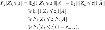
which is the announced result. □
This result is very useful for risk management. If you take for z the (1−ɛ)th quantile of Z k under P 1 then the probability that Z k is less than z under P 2 is at least equal to (1−ɛ mort )(1−ɛ). Taking ɛ mort =ɛ=1 percent for example, shows that the 99th percentile of Z k under P 1 is at least equal to the 98.01th percentile of Z k under P 2.

 be the indicator of E, that is,
  is E is realized, and 0 otherwise. Then, denoting as 𝔼
i
the mathematical expectation taken under P
i
, for i=1, 2,
is E is realized, and 0 otherwise. Then, denoting as 𝔼
i
the mathematical expectation taken under P
i
, for i=1, 2, 
Remark 2
-
Property 1 can be extended to the expectation of any non-increasing function of the T i 's. It is indeed easy to see that considering any non-negative non-increasing function g : ℝn → ℝ+, we have


Ruin probability
Let U t be the surplus of the insurance company at time t. Starting from U 0=u, the surplus obeys to the dynamics

where L 0=n by convention, where L t denotes the (random) number of survivors at time t among the initial n annuitants, and where r t is the (deterministic) interest rate earned on the reserve during period t (from t−1 to t).
Let us denote the ruin probability at horizon k computed under first-order basis (i=1) and under second-order basis (i=2) as

where  is the non-ruin probability. We thus work conditionally on the initial reserve u, for a given initial number n of annuitants all aged x
0 at issuance (in calendar year t
0).
is the non-ruin probability. We thus work conditionally on the initial reserve u, for a given initial number n of annuitants all aged x
0 at issuance (in calendar year t
0).
For any horizon k, the non-ruin probability can be expressed as

Coming back to (3), we see that U t <0 → U t+j <0 for any j=1, 2, …, which in turn implies that the non-ruin probability can be expressed as

Computing the non-ruin probability at horizon k then amounts to evaluate the distribution function of Z k .
Let u be the initial capital such that the ultimate ruin probability  is at most ɛ
solv
for a portfolio of n annuitants. Note that the number of annuities comprised in the portfolio is an element of the computation. Specifically, we consider the random variable , and we determine its 1−ɛ
solv
quantile under P
1.
is at most ɛ
solv
for a portfolio of n annuitants. Note that the number of annuities comprised in the portfolio is an element of the computation. Specifically, we consider the random variable , and we determine its 1−ɛ
solv
quantile under P
1.
The ruin probability under the second-order mortality basis is difficult to evaluate in an analytical way, but we can provide the following easy-to-compute lower bound. Specifically, considering (4), Property 1 allows us to write

For instance, taking ɛ mort =ɛ solv =1 percent gives a ruin probability of at most 1.99 percent.
Numerical illustration
Context
This section discusses a practical example. We consider individuals buying a life annuity at the age of 65 in year 2005. We can think of people getting retired and desiring to convert their pension fund benefits into periodic payments. In this section, we consider Belgian males aged 65 in year 2005. We take in all the computations ω=100.
We use the 2005 zero coupon yield curve published by Eurostat (for more details, we refer the interested reader to the website http://epp.eurostat.cec.eu.int) to obtain the discount factors used for the numerical illustration. Specifically, the r t 's correspond to the forward rates deduced from the prices of Euro zero coupon bonds. The Eurostat curve shows the structure of interest rates for maturities of one year up to 30 years. The bonds are identified as government issues to guarantee their quality. They are thus appropriate to use by annuity providers (being non-defaultable and having the same currency as the insurer's liabilities).
Mortality projection
We apply the Poisson modeling to the general population data of Belgium. The ages considered here range from 65 to 100, and the observation period is 1950–2002. All the data are available from the Human Mortality Database (maintained by the University of California, Berkeley, U.S.A., and the Max Planck Institute for Demographic Research, Germany), http://www.mortality.org (data downloaded in October 2006).
The higher variability observed at advanced ages rules out the least-squares approach to estimating the Lee–Carter parameters , β x and κ t (since it assumes a constant variance across ages) unless the mortality surface is previously closed as explained in Denuit and Goderniaux (2005). Here, we resort to the Poisson maximum likelihood approach to estimating the 's, β x 's and κ t 's, allowing for heteroskedasticity.
Applying the methodology proposed by Booth et al. (2002) to Belgian males yields an optimal calibration period starting in 1974. The ad hoc method of Denuit and Goderniaux (2005) suggests that we could start the fitting period in 1970, since the adjustment coefficient peaks around 1970. Therefore, we focus on the period 1970–2002 (Figure 1).

Estimated 's, β x 's and κ t 's obtained for the optimal fitting period 1970–2002.
Let us now model the time index κ t . As in the Lee–Carter methodology the time factor κ t is intrinsically viewed as a stochastic process. Box–Jenkins techniques are therefore used to estimate and forecast κ t within an ARIMA times series model. First, the κ t 's are differenced, to remove the downward linear trend. Considering the first differences of the time index, the autocorrelation functions and partial autocorrelation functions (which both tail off) clearly suggests that an ARIMA(0,1,0) process is appropriate. Running a Shapiro–Wilk test yields a P-value of 0.2358, which indicates that the residuals seem to be approximately Normal. The corresponding Jarque–Bera statistics is 0.4734, which confirms that there is no significant departure from Normality. The random walk with drift model outperforms its competitor on the basis of standard information criteria. The ARIMA(0,1,0) estimated parameters for the period 1970–2002 are θ̂=−0.4169175 and ς̂ 2=0.3333644. The projected κ t 's are then obtained from last κ 2002 by adding a linear trend with slope θ̂.
First-order mortality basis
We are now in a position to determine the conservative life table. The criterion is that the random future life table should not produce smaller death rates than the conservative life table with probability at least 99 percent (corresponding to ɛ mort =11 percent). This gives π=0.9320154. This value of π has been found using the qmvnorm function of the R package mvtnorm.
This gives a pure life annuity premium amount of 11.62939, to be compared with 11.37335 obtained with the projected life table. The increase in the premium amount is rather moderate. This can be explained by the Gaussian modeling for the time index together with the effect of discounting. The distribution function of the present values  of the life annuity payments for policyholder i is depicted in Figure 2 (left panel) where T
i
obeys to the first-order life table. The right panel of Figure 2 describes the distribution function obtained after discretization.
of the life annuity payments for policyholder i is depicted in Figure 2 (left panel) where T
i
obeys to the first-order life table. The right panel of Figure 2 describes the distribution function obtained after discretization.

Distribution function of the present values of the annuity payments  (on the left) and its discretized version (on the right).
Ruin probabilities
The distribution of Z 35 can easily be computed as explained in the previous section. Figure 3 gives the probability mass function and the distribution function for n=10, 20 and 30. Imposing a non-ruin probability of 99 percent (i.e., ɛ solv =0.01) under P 1 requires an initial capital u(10, 1%, 1%)=152, u(20, 1%, 1%)=287, and u(30, 1%, 1%)=417.9, respectively, under P 1. These values correspond to ruin probabilities of at most 2 percent under P 2. Increasing the number of policies clearly reduces the amount of capital per policy, as expected.

Probability mass functions (left panels) and corresponding distribution functions (right panels) of Z 35 under P 1 for n=10 (top), 20 (middle) and 30 (bottom).
Let us now augment this preliminary set of results to indicate how u depends on ɛ mort and ɛ solv under P 1. To this end, we have computed the values displayed in the next table. illustration

These values correspond to the capital needed to have a ruin probability of at most ɛ solv under P 1 (when P 1 corresponds to ɛ mort ), divided by the number n of policies. As expected for fixed ɛ solv , these values decrease as ɛ mort increases. Similarly, for fixed ɛ mort , these values decrease as ɛ solv increases. Some values coincide because of the discrete nature of the underlying distribution. Note that combining ɛ mort =0.5 percent with ɛ solv =0.5 percent gives a ruin probability of at most 1 percent under P 2.
Conclusion
In this paper, first-order mortality bases for life annuity contracts, using a conservative life table corresponding to a high-longevity scenario (determined by the ɛ mort probability level). Assuming that the remaining life times are mutually independent, the computation of ruin probabilities is then straightforward from Panjer algorithm. We prove that this approach allows us to control the ruin probability in the second-order mortality basis.
In this paper, we have disregarded the sampling errors in the Lee–Carter parameters , β x and κ t , and in the ARIMA parameters. The two sources of uncertainty that have to be combined are the sampling fluctuation in the , β x , and κ t parameters, and the forecast error in the κ t parameters. To this end, Brouhns et al. (2002a, 2002b) sampled directly from the approximate multivariate Normal distribution of the maximum likelihood estimators , β̂, κ. Brouhns et al. (2005) sampled from the death counts (under a Poisson error structure). Specifically, the bootstrapped death counts are obtained by applying a Poisson noise to the observed numbers of deaths. The bootstrapping procedure can also be achieved in a number of alternative ways. We refer to Renshaw and Haberman (2008) for a detailed study.
For individual death rate forecasts, we know from Lee and Carter (1992, Appendix B) that confidence intervals based on κ t alone are a reasonable approximation only for forecast horizons greater than 10–25 years. For long-run forecasts (35 years in the numerical illustration), the error in forecasting the mortality index clearly dominates the errors in fitting the mortality matrix.
References
Booth, H., Maindonald, J. and Smith, L. (2002) ‘Applying Lee–Carter under conditions of variable mortality decline’, Population Studies 56: 325–336.
Brouhns, N., Denuit, M. and Van Keilegom, I. (2005) ‘Bootstrapping the Poisson log-bilinear model for mortality projection’, Scandinavian Actuarial Journal 2005 (3): 212–224.
Brouhns, N., Denuit, M. and Vermunt, J.K. (2002a) ‘A Poisson log-bilinear approach to the construction of projected lifetables’, Insurance: Mathematics and Economics 31: 373–393.
Brouhns, N., Denuit, M. and Vermunt, J.K. (2002b) ‘Measuring the longevity risk in mortality projections’, Bulletin of the Swiss Association of Actuaries 2002 (2): 105–130.
Cossette, H., Delwarde, A., Denuit, M., Guillot, F. and Marceau, E. (2007) ‘Pension plan valuation and dynamic mortality tables’, North American Actuarial Journal 11: 1–34.
Czado, C., Delwarde, A. and Denuit, M. (2005) ‘Bayesian Poisson log-bilinear mortality projections’, Insurance: Mathematics & Economics 36: 260–284.
Delwarde, A., Denuit, M. and Eilers, P. (2007) ‘Smoothing the Lee–Carter and Poisson log-bilinear models for mortality forecasting: A penalized log-likelihood approach’, Statistical Modelling 7: 29–48.
Delwarde, A., Denuit, M. and Partrat, Ch. (2007) ‘Negative binomial version of the Lee–Carter model for mortality forecasting’, Applied Stochastic Models in Business and Industry 23: 385–401.
Denuit, M. and Frostig, E. (2007a) ‘Association and heterogeneity of insured lifetimes in the Lee–Carter framework’, Scandinavian Actuarial Journal 107: 1–19.
Denuit, M. and Frostig, E. (2007b) Life insurance mathematics with random life tables, working paper 07-07, Institut des Sciences Actuarielles, Université Catholique de Louvain, Louvain-la-Neuve, Belgium.
Denuit, M. and Goderniaux, A.-C. (2005) ‘Closing and projecting lifetables using log-linear models’, Bulletin of the Swiss Association of Actuaries 2005: 29–49.
De Pril, N. (1985) ‘Recursions for convolutions of arithmetic distributions’, ASTIN Bulletin 15: 135–139.
Frostig, E., Haberman, S. and Levikson, B. (2003) ‘Generalized life insurance: Ruin probabilities’, Scandinavian Actuarial Journal 2: 136–152.
Lee, R.D. and Carter, L. (1992) ‘Modelling and forecasting the time series of US mortality’, Journal of the American Statistical Association 87: 659–671.
Panjer, H.H. and Wang, S. (1993) ‘On the stability of recursive formulas’, ASTIN Bulletin 23: 227–258.
Renshaw, A.E. and Haberman, S. (2003) ‘Lee–Carter mortality forecasting with age specific enhancement’, Insurance: Mathematics & Economics 33: 255–272.
Renshaw, A.E. and Haberman, S. (2008) ‘On simulation-based approaches to risk measurement in mortality with specific reference to Poisson Lee–Carter modelling’, Insurance: Mathematics & Economics, available online, doi:10.1016/j.insmatheco.2007.08.009.
Wang, S. (1995) ‘Insurance pricing and increased limits ratemaking by proportional hazard transforms’, Insurance: Mathematics & Economics 17: 43–54.
Acknowledgements
We thank the three anonymous referees for useful comments, which significantly improved the original manuscript and helped to clarify the results. Michel Denuit acknowledges the financial support of the Communauté Française de Belgique under contract “Projet d’Actions de Recherche Concertées ARC 04/09-320”, as well as the financial support of the Banque Nationale de Belgique under grant “Risk Measures and Economic Capital”.
Author information
Authors and Affiliations
Rights and permissions
About this article
Cite this article
Denuit, M., Frostig, E. First-Order Mortality Basis for Life Annuities. Geneva Risk Insur Rev 33, 75–89 (2008). https://doi.org/10.1057/grir.2008.9
Published:
Issue Date:
DOI: https://doi.org/10.1057/grir.2008.9