A general model-checking procedure for semiparametric accelerated failure time models

Abstract

We propose a set of goodness-of-fit tests for the semiparametric accelerated failure time (AFT) model, including an omnibus test, a link function test, and a functional form test. This set of tests is derived from a multi-parameter cumulative sum process shown to follow asymptotically a zero-mean Gaussian process. Its evaluation is based on the asymptotically equivalent perturbed version, which enables both graphical and numerical evaluations of the assumed AFT model. Empirical p-values are obtained using the Kolmogorov-type supremum test, which provides a reliable approach for estimating the significance of both proposed un-standardized and standardized test statistics. The proposed procedure is illustrated using the rank-based estimator but is general in the sense that it is directly applicable to some other popular estimators such as induced smoothed rank-based estimator or least-squares estimator that satisfies certain properties. Our proposed methods are rigorously evaluated using extensive simulation experiments that demonstrate their effectiveness in maintaining a Type I error rate and detecting departures from the assumed AFT model in practical sample sizes and censoring rates. Furthermore, the proposed approach is applied to the analysis of the Primary Biliary Cirrhosis data, a widely studied dataset in survival analysis, providing further evidence of the practical usefulness of the proposed methods in real-world scenarios. To make the proposed methods more accessible to researchers, we have implemented them in the R package afttest, which is publicly available on the Comprehensive R Archive Network.

Appendix

We prove Theorems 1 and 2 for the non-smooth rank-based estimator, . We impose the following regularity conditions C1–C7. These conditions are also specified in Lin et al. (1998) and Novák (2013).

• C1 $\varvec{Z}_{i}, i=1, \cdots , n$ are bounded.

• C2 $\left( N_{i}, C_{i}, \varvec{Z}_{i} \right) , i=1, \cdots , n$ are i.i.d..

• C3 $\psi _{n} \left( t, \varvec{\beta }_{0}\right) , E_{n} \left( t, \varvec{\beta }_{0} \right) , E_{n}^{\left( \pi \right) } \left( t, \varvec{\beta }_{0}\right)$, and $n^{-1} S_{n}^{\left( \pi \right) } \left( t, \varvec{\beta }_{0}\right)$ have bounded variations and converge almost surely to the continuous functions $\psi _{\infty }, E_{\infty }, E_{\infty }^{\left( \pi \right) }$, and $S_{\infty }^{\left( \pi \right) }$, respectively.

• C4 $C_{i} \exp \left( \varvec{Z}^{\top }_{i} \beta _{0} \right)$ have a uniformly bounded density and $\Lambda _{0} \left( \cdot \right)$ has a bounded second derivative.

• C5 $f_{\pi } \left( t, \varvec{z}\right)$ and $g_{\pi } \left( t, \varvec{z}\right)$ have bounded variations and converge almost surely to $f_{\infty }^{\left( \pi \right) } \left( t, \varvec{z}\right)$ and $g_{\infty }^{\left( \pi \right) } \left( t, \varvec{z}\right)$, respectively.

• C6 The kernel estimate of $\widehat{f}_{n}^{\left( 0 \right) } \left( t \right)$ and $\widehat{g}_{n}^{\left( 0 \right) } \left( t \right)$ have bounded variations and converge in probability uniformly to $f^{\left( 0 \right) } \left( t \right)$ and $g^{\left( 0 \right) } \left( t \right)$, respectively.

• C7 $\varvec{\Omega } = \int _{0}^{\infty } \psi _{n} \left( t \right) {\mathbb {E}} [ Y_{1} \left( t,\varvec{\beta }_{0} \right) \left\{ \varvec{Z}_{1} - E_{\infty } \left( t \right) \right\} \left\{ \varvec{Z}_{1} - E_{\infty }\left( t \right) \right\} ^{\top }] d \left( \lambda _{0} \left( t \right) t \right)$ is full rank.

As mentioned in Sect. 3, these results are also applicable to the other estimators such as the induced smoothed rank-based estimator, , and least-squares estimator, . For , the results remain identical mainly due to the asymptotic equivalence of the limiting distributions of and (Johnson and Strawderman 2009). For , the $h_{i}(\cdot )$ in the asymptotic representation for , a sum of integrated martingale residuals, is different from those for or . Its specific form is presented in (A7) of Jin et al. (2006, Appendix). The asymptotic covariance function for will have a different form due to the differences of $\varvec{\Omega }$ and $h_{i}(\cdot )$ in Theorem 1 that are specific to . $\varvec{\Omega }$ in C7 will also be changed when is considered.

1.1 A.1 Proof of Theorem 1

We first state the following Results 1–4, frequently used in the proofs of Theorems 1 and 2, derived in Lin et al. (1998) and Novák (2013). Results 1 and 2 are the asymptotic expansion results of and $\widehat{\Lambda }_{n} \left( t, \varvec{\beta }\right)$ about $\varvec{\beta }_{0}$, respectively (Lin et al. 1998). Specifically, under C1–C7,

Result 1

For as $n \rightarrow \infty$,

Result 2

For as $n \rightarrow \infty$,

$$\begin{aligned}&\sup _{ \Vert \varvec{\beta }- \varvec{\beta }_{0} \Vert < d_{n} } \Vert n^{\frac{1}{2}} \left\{ \widehat{\Lambda }_{n} \left( t , \varvec{\beta }\right) - \widehat{\Lambda }_{n} \left( t , \varvec{\beta }_{0} \right) \right\} \\ {}&\quad - \varvec{\kappa }^{\top } \left( t \right) n^{\frac{1}{2}} \left( \varvec{\beta }- \varvec{\beta }_{0} \right) \Vert = o_{p} \left( 1 \right) \end{aligned}$$

where

$$\begin{aligned} \varvec{\kappa } \left( t \right) = - \int _{0}^{t} E_{\infty } \left( s \right) d \left( \lambda _{0} \left( s \right) s \right) . \end{aligned}$$

Results 3 and 4 are the asymptotic expansion results of the normalized weighted sum processes of $N_{i} \left( t, \varvec{\beta }\right)$ and $Y_{i} \left( t, \varvec{\beta }\right)$ about $\varvec{\beta }_{0}$, respectively (Novák 2013, Lemma 6.1; p.53). Specifically, under C1–C7,

Result 3

For as $n \rightarrow \infty$,

$$\begin{aligned}&\sup _{t \in \left[ 0, \infty \right) , \Vert \varvec{\beta }- \varvec{\beta }_{0} \Vert < d_{n}} \Vert n^{-\frac{1}{2}} \sum _{i=1}^{n} \pi _{i} \left( \varvec{Z}\right) \left( N_{i} \left( t , \varvec{\beta }\right) - N_{i} \left( t , \varvec{\beta }_{0} \right) \right) \\ {}&\qquad + f_{n}^{\left( \pi \right) } \left( t, \varvec{z}\right) ^{\top } n^{\frac{1}{2}} \left( \varvec{\beta }- \varvec{\beta }_{0} \right) \Vert = o_{p} \left( 1 \right) . \end{aligned}$$

Result 4

For as $n \rightarrow \infty$,

$$\begin{aligned}&\sup _{t \in \left[ 0, \infty \right) , \Vert \varvec{\beta }- \varvec{\beta }_{0} \Vert < d_{n} } \Vert n^{-\frac{1}{2}} \sum _{i=1}^{n} \pi _{i} \left( \varvec{z}\right) \left( Y_{i} \left( t , \varvec{\beta }\right) - Y_{i} \left( t , \varvec{\beta }_{0} \right) \right) \\&\qquad + g_{n}^{\left( \pi \right) } \left( t , \varvec{z}\right) ^{\top } n^{\frac{1}{2}} \left( \varvec{\beta }- \varvec{\beta }_{0} \right) \Vert \\&\quad = o_{p} \left( 1 \right) . \end{aligned}$$

First, we show that follows asymptotically a zero-mean Gaussian process. This part of the proof simply follows the proof in Appendix of Novák (2013). By using the definition of the martingale residual, we have

It follows from applying Result 3 that

Using Results 1 and 2 and under the assumption that $\varvec{\Omega }$ is full rank, we have

Then, by applying Result 4 and the asymptotic expansion result , we have

Denote

For fixed t and $\varvec{z}$, each of the processes is a sum of i.i.d. quantities having a zero mean. The multivariate central limit theorem establishes the finite-dimensional convergence of $\left( V_{n}^{t}, V_{n}^{\varvec{Z}}, V_{n}^{\pi } \right)$. , , and , $i =1, \cdots , n$ are manageable (Pollard 1990, p38) since they can be expressed as sums and products of monotone functions. Then, it follows from the functional central limit theorem (Pollard 1990)) that $\left( V_{n}^{t}, V_{n}^{\varvec{Z}}, V_{n}^{\pi } \right)$ is tight and converges weakly to a zero-mean Gaussian process, denoted as $\left( V_{\infty }^{t}, V_{\infty }^{\varvec{Z}}, V_{\infty }^{\pi } \right)$. By the Skorohod-Dudley-Wichura theorem (Shorack and Wellner 2009, p47), there exists an equivalent process $\left( V_{n}^{t}, V_{n}^{\varvec{Z}}, V_{n}^{\pi } \right)$ in an alternative probability space that the weak convergence is strengthened to almost sure convergence. Combining these results with the almost sure convergence results of $\psi _{n} \left( t, \varvec{\beta }_{0}\right)$, $E_{n} \left( t, \varvec{\beta }_{0}\right)$, $E_{n}^{\left( \pi \right) }\left( t, \varvec{\beta }_{0}\right)$, and $n^{-1} S_{n}^{\left( \pi \right) }\left( t, \varvec{\beta }_{0}\right)$ to continuous functions $\psi _{\infty }$, $E_{\infty }$, $E_{\infty }^{\left( \pi \right) }$, and $S_{\infty }^{\left( \pi \right) }$, respectively, we have the following almost sure convergence results:

• 1. 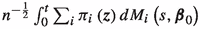converges to $\int _{0}^{t} d V_{\infty }^{\pi }$

• 2. 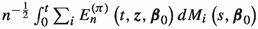converges to $\int _{0}^{t} E_{\infty }^{\left( \pi \right) } \left( s,\varvec{\beta }_{0} \right) d V_{\infty }^{\varvec{Z}} \left( s \right) ;$

• 3. 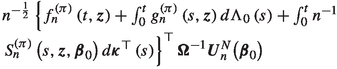converges to $\left\{ f_{\infty }^{\left( \pi \right) } \left( t \right) + \int _{0}^{t} g_{\infty }^{\left( \pi \right) } \left( s \right) d \Lambda _{0} \left( s \right) + \int _{0}^{t} S_{\infty }^{\left( \pi \right) } \left( s, \varvec{z}, \varvec{\beta }_{0} \right) d \varvec{\kappa }^{\top }\right.$$\left. \left( s \right) \right\} ^{\top } \varvec{\Omega }^{-1}\left\{ \int _{0}^{\infty } \psi _{\infty } \left( s \right) d V_{\infty }^{\varvec{Z}} - \int _{0}^{\infty } \psi _{\infty } \left( s \right) E_{\infty } \left( s,\varvec{\beta }_{0} \right) \right.$ $\left. d V_{\infty }^{t} \right\} .$

Note that, in Jin et al. (2003), it was shown that , i.e., a sum of integrated martingales where $\psi _{\infty }\left( s \right) \left\{ \varvec{Z}_{i} - E_{\infty } \left( s, \varvec{\beta }_{0} \right) \right\}$ are nonrandom functions.

In summary, as $n \rightarrow \infty$, converges weakly to

$$\begin{aligned}&\int _{0}^{t} dV_{\infty }^{\varvec{Z}} - \int _{0}^{t} E_{\infty } \left( s, \varvec{\beta }_{0} \right) dV_{\infty }^{t} \\&\quad - \varvec{\nu }^{\top } \left( t, \varvec{z}\right) \varvec{\Omega }^{-1}\left\{ \int _{0}^{\infty } \psi _{\infty } \left( s \right) dV_{\infty }^{\varvec{Z}} \right. \\&\quad \left. - \int _{0}^{\infty } \psi _{\infty } \left( s \right) E_{\infty } \left( s, \varvec{\beta }_{0} \right) dV_{\infty }^{t} \right\} , \end{aligned}$$

a Gaussian process with the zero-mean and the covariance function being

where $\varvec{\nu } \left( t, \varvec{z}\right) = f_{\infty }^{\left( \pi \right) } \left( t,\varvec{z}\right) + \int _{0}^{t} g_{\infty }^{\left( \pi \right) } \left( s, \varvec{z}\right) d \Lambda _{0} \left( s \right) + \int _{0}^{t} S_{\infty }^{\left( \pi \right) } \left( s, \varvec{z}, \varvec{\beta }_{0} \right) d \varvec{\kappa }^{\top } \left( t \right)$.

Second, we claim that the omnibus test based on is consistent against the general alternative that there does not exist a constant vector $\varvec{\beta }$ and a function $\lambda _{0} \left( \cdot \right)$ such that $\lambda (t | \varvec{Z}) = \lambda _{0} \left( t \cdot g \left( \varvec{Z}\right) \right) g \left( \varvec{Z}\right)$, generalized hazard function, for almost all $t > 0$ and $\varvec{z}$ generated by the random vector $\varvec{Z}$.

We first decompose into two parts:

(9)

Then, it follows from the Strong Law of Large Numbers (SLLN) and Lin et al. (1998, Theorem 2; p.616), (9) is asymptotically equivalent to

(10)

Let $H \left( \varvec{z}\right)$ denote the distribution of $\varvec{Z}_{i}$. Then, the first term of (10) can rewritten as

The last equality above comes from $\lambda (t | \varvec{Z}) = \lambda _{0} \left( t \cdot g \left( \varvec{Z}\right) \right) g \left( \varvec{Z}\right)$. Likewise, the second term of (10) can be written as

Combining these two results, (10) reduces to

(11)

Under the alternative hypothesis, and converge to $\varvec{\beta }_{\infty }^{\star }$ and $\int \lambda _{0}^{\star } (s, \varvec{\beta }_{\infty }^{\star }) ds$, respectively, and $g \left( Z; \varvec{\beta }_{\infty }^{\star } \right) \ne \exp \left( Z^{\top } \varvec{\beta }_{\infty }^{\star } \right)$. Therefore, (11) converges to

$$\begin{aligned}&\int _{-\infty }^{\varvec{z}} \int _{0}^{t} \ell \left( \varvec{v}\right) Y_{i} \left( s,\varvec{\beta }_{\infty }^{\star } \right) \exp \left( - \varvec{v}^{\top } \varvec{\beta }_{\infty }^{\star } \right) \\&\quad \left\{ \frac{g \left( \varvec{v}; \varvec{\beta }_{\infty }^{\star } \right) }{\exp \left( - \varvec{v}^{\top } \varvec{\beta }_{\infty }^{\star } \right) } - \frac{\lambda _{0}^{\star } \left( s \cdot \exp \left( - \varvec{v}^{\top } \varvec{\beta }_{\infty }^{\star } \right) \right) }{\lambda _{0} \left( s \cdot g \left( \varvec{v}; \varvec{\beta }_{\infty }^{\star } \right) \right) } \right\} \\&\quad \lambda _{0} \left( s \cdot g \left( \varvec{v}; \varvec{\beta }_{\infty }^{\star } \right) \right) d s d H \left( \varvec{v}\right) . \end{aligned}$$

By Hardy et al. (1952, p.136) and in Lin et al. (1993, Appendix 3), as $n \rightarrow \infty$,

almost surely. For the maximizer of $g \left( \varvec{z}; \varvec{\beta }_{\infty }^{\star } \right) / \exp \left( {-}\varvec{z}^{\top } \varvec{\beta }_{\infty }^{\star } \right)$, say $\varvec{z}_{\dag }$, we have

$$\begin{aligned}&\left\{ \frac{g \left( \varvec{z}_{\dag } ; \varvec{\beta }_{\infty }^{\star } \right) }{\exp \left( - \varvec{z}_{\dag }^{\top } \varvec{\beta }_{\infty }^{\star } \right) } \right\} \\&\quad - \frac{ \int \exp \left( -\varvec{z}^{\top } \varvec{\beta }_{\infty }^{\star } \right) \left\{ \frac{g \left( \varvec{z}; \varvec{\beta }_{\infty }^{\star } \right) }{\exp \left( -\varvec{z}^{\top } \varvec{\beta }_{\infty }^{\star } \right) } \right\} Y_{i} \left( t, \varvec{\beta }_{\infty }^{\star } \right) dH \left( \varvec{z}\right) }{\int \exp \left( -\varvec{z}^{\top } \varvec{\beta }_{\infty }^{\star } \right) Y_{i} \left( t, \varvec{\beta }_{\infty }^{\star } \right) dH\left( \varvec{z}\right) } > 0. \end{aligned}$$

It shows that the test statistic is consistent against the general alternative as we stated above.

Table 5 Rejection rates under the nominal level of 0.05 testing the exponentiality of the model $\lambda \left( t | Z \right) = \lambda _{0} \left( t \right) \exp \left( 0.3 Z \right)$

1.2 A.2 Proof of Theorem 2

To show that is asymptotically identically distributed as the test statistic based on non-smoothed score process where

Under Results 1 and 2,

Since , we observe that shares the same components as . Note that $\varvec{\beta }_{0}$, , $f_{n}^{\left( \pi \right) } \left( t, \varvec{z}\right)$, and $g_{n}^{\left( \pi \right) } \left( t, \varvec{z}\right)$ can be replaced by , , $\widehat{f}_{n}^{\left( \pi \right) } \left( t, \varvec{z}\right)$, and $\widehat{g}_{n}^{\left( \pi \right) } \left( t, \varvec{z}\right)$, respectively. In addition, the resampled martingale residuals have the same distribution as , and the kernel estimates of $f^{\left( 0 \right) }$ and $g^{\left( 0 \right) }$ converge uniformly to their true densities. Consequently, exhibits the same limiting finite-dimensional distributions as , and its tightness follows the same arguments as for .

1.3 A.3 Timing results for the simulation studies and real data analysis

For the simulation studies and real data analysis, we used parallel computing on a high-performance computing environment, the University of Florida HiPerGator 3.0 cluster (70,320 cores, with 8GB RAM per core). Running time depends on many factors such as the sample size, the number of covariates, complexity of the data structure, etc. Under Simulation Scenario 2, Table 4 presents the running timing results for different sample sizes and values of $\gamma$.

1.4 A.4. Additional simulation experiments

We conducted additional simulation experiments to investigate various underlying parametric distributions, following the setup outlined in Lin and Spiekerman (1996, Chapter 5). The objective was to test the exponentiality assumption under the proportional hazards (PH) model, where the hazard function is defined as $\lambda \left( t | Z \right) = \lambda _{0} \left( t \right) \exp \left( 0.3 Z \right)$, with the covariate Z following a standard normal distribution. To evaluate the type I error rate and power, we generated baseline failure times from two distributions: the Weibull distribution with the survival function $S \left( t \right) = \exp \left( - t^{\rho } \right)$ with $\rho =$ 1, 0.5 and 2, and the log-normal distribution with the survival function $S \left( t \right) = 1 - \Phi \left( - \sigma ^{-1} \log t \right)$ with $\sigma = 0.5$ and 3. Censoring times were generated from independent uniform random variables within the interval $\left( 0, \tau \right)$. The value of $\tau$ was chosen to achieve the desired censoring rates of 25%, 50% and 75% in each simulation sample. We set the sample sizes to $n =$ 50, 100 and 200. For each configuration, we applied our proposed semiparametric test procedures with 200 approximated sample paths from the null model, repeating this procedure 1,000 times. The rejection rates (p-values) under our proposed procedure and the parametric test procedure by Lin and Spiekerman (1996) are presented in Table 5.

Under our proposed approach (“stdmis"), the rejection rates consistently remained low around 0.05 or less in most cases considered. In contrast, the parametric approach (ls) produced values close to 0.05 only when considering the exponential distribution with a baseline hazard function of 1 ($\text {W} \left( 1 \right)$). When other distributions were considered, the corresponding rejection rates increased, with some of them even approaching 1 in cases of low censoring rates (25%) or larger sample sizes ($n =$ 100 or 200). These findings are not surprising given the nature of the hypotheses for the two approaches.

It is important to note that there are differences in the hypotheses between the parametric test and the proposed semiparametric test. In the parametric test by Lin and Spiekerman (1996), the null hypothesis assumes a PH model with an exponential distribution, where the baseline hazard is equal to 1, i.e., $H_{0}: \lambda \left( t | Z \right) = \exp \left( 0.3 Z \right)$. The alternative hypothesis considers a PH model with other specific distributions, assuming specified parameter values, such as Weibull distributions with $\rho =$ 0.5 or 2 ($\text {W} (0.5)\hbox { or }\text {W} (2)$), or log-normal distributions with $\sigma =$ 0.5 or 3 ($\text {LN}(0.5)$ or $\text {LN}(3)$). On the other hand, for our proposed test, the null hypothesis is an AFT model with a single covariate Z, i.e., $H_{0}: \text {Data follows an AFT model with a single covariate }Z$. Therefore, direct comparison between the two tests is not straightforward. For example, in the parametric approach, only the unit exponential distribution, $\text {W} (1)$, is considered the correct specification. In contrast, for our proposed approach, any Weibull distribution (regardless of the value of the shape parameter) is considered a correct specification, as PH models with Weibull baseline hazards also satisfy the assumptions of the AFT model. Consequently, it is not surprising that the results remain under control at the nominal significance level for any Weibull distributions.

The log-normal distributional assumption for the baseline hazard function in the current PH model does not precisely align with the AFT assumption. This constitutes a misspecification in the baseline hazard function, failing to account for the time-transformed feature. Consequently, we anticipate that an AFT model may only partially approximate these distributions, resulting in lower corresponding statistical power. It is important to note that a single probability density can often be well-represented by an entirely different family of densities Cavallo et al. (2012). Furthermore, distinguishing between Weibull and log-normal distributions becomes challenging when the censoring rate is high or the sample sizes are small (Cain 2002). Except for the $\text {LN}(0.5)$ case with $n=200$ and censoring rates of 25% or 50%, all estimated powers are approximately 0.05 or lower. Consequently, we conducted additional simulation experiments with a sample size of 500 to assess whether the statistical power of the proposed test improves. As expected, for the log-normal cases, the powers increase and can be as high as 0.190 (LN(0.5) with a 25% censoring rate). Overall, it is worth noting that the powers still appear considerably lower than those obtained by the parametric approach proposed by Lin and Spiekerman (1996). These differences can be attributed to the nature of the semiparametric procedure and, to some extent, the non-direct comparability of the hypotheses.

References

Bae, W., Choi, D., Yan, J., Kang, S.: afttest: model diagnostics for accelerated failure time models. R package version 4.3.2.2. https://cran.r-project.org/web/packages/afttest/index.html (2022)
Bagdonavičius, V.B., Levuliene, R.J., Nikulin, M.S.: Chi-squared goodness-of-fit tests for parametric accelerated failure time models. Commun. Stat.-Theory Methods 42, 2768–2785 (2013)
Balakrishnan, N., Chimitova, E., Galanova, N., Vedernikova, M.: Testing goodness of fit of parametric aft and ph models with residuals. Commun. Stat.-Simul. Comput. 42, 1352–1367 (2013)
Barlow, W.E., Prentice, R.L.: Residuals for relative risk regression. Biometrika 75, 65–74 (1988)
Brown, B.M., Wang, Y.: Induced smoothing for rank regression with censored survival times. Stat. Med. 26, 828–836 (2006). https://doi.org/10.1002/sim.2576
Buckley, J., James, I.: Linear regression with censored data. Biometrika 66, 429–436 (1979)
Cain, S.R.: Distinguishing between lognormal and weibull distributions [time-to-failure data]. IEEE Trans. Reliab. 51, 32–38 (2002)
Cavallo, A., Rosenthal, B., Wang, X., Yan, J.: Treatment of the data collection threshold in operational risk: a case study using the lognormal distribution. J. Operat. Risk 7(1), 3–38 (2012). https://doi.org/10.21314/jop.2012.101
Chiou, S., Kang, S., Yan, J.: Rank-based estimating equations with general weight for accelerated failure time models: an induced smoothing approach. Stat. Med. 34, 1495–1510 (2015)
Chiou, S.H., Kang, S., Kim, J., Yan, J.: Marginal semiparametric multivariate accelerated failure time model with generalized estimating equations. Lifetime Data Anal. 20, 599–618 (2014)
Chiou, S.H., Kang, S., Yan, J.: Fitting accelerated failure time models in routine survival analysis with r package aftgee. J. Stat. Softw. 61, 1–23 (2014)
Chiou, S.H., Kang, S., Yan, J.: Semiparametric accelerated failure time modeling for clustered failure times from stratified sampling. J. Am. Stat. Assoc. 110, 621–629 (2015). https://doi.org/10.1080/01621459.2014.917978
Cockeran, M., Meintanis, S.G., Santana, L., Allison, J.S.: Goodness-of-fit testing of survival models in the presence of type-ii right censoring. Comput. Statistics 36, 977–1010 (2021)
Cox, D.R.: Regression models and life-tables. J. Roy. Stat. Soc.: Ser. B (Methodol.) 34, 187–202 (1972). https://doi.org/10.1111/j.2517-6161.1972.tb00899.x
Diehl, S., Stute, W.: Kernel density and hazard function estimation in the presence of censoring. J. Multivar. Anal. 25, 299–310 (1988)
Ding, Y., Nan, B.: Estimating mean survival time: when is it possible? Scand. J. Stat. 42, 397–413 (2015)
Fleming, T.R., Harrington, D.P.: Counting processes and survival analysis, vol. 625. John Wiley & Sons (2013)
Hardy, G., Littlewood, J., Pólya, G.: Inequalities. Cambridge Mathematical Library, Cambridge University Press https://books.google.com/books?id=t1RCSP8YKt8C (1952)
Huang, C.-Y., Luo, X., Follmann, D.A.: A model checking method for the proportional hazards model with recurrent gap time data. Biostatistics 12, 535–547 (2011). https://doi.org/10.1093/biostatistics/kxq071
Jin, Z., Lin, D., Wei, L., Ying, Z.: Rank-based inference for the accelerated failure time model. Biometrika 90, 341–353 (2003)
Jin, Z., Lin, D.Y., Ying, Z.: On least-squares regression with censored data. Biometrika 93, 147–161 (2006)
Johnson, L.M., Strawderman, R.L.: Induced smoothing for the semiparametric accelerated failure time model: asymptotics and extensions to clustered data. Biometrika 96, 577–590 (2009)
Lee, C.H., Ning, J., Shen, Y.: Model diagnostics for the proportional hazards model with length-biased data. Lifetime Data Anal. 25, 79–96 (2019)
Li, J., Scheike, T.H., Zhang, M.-J.: Checking fine and gray subdistribution hazards model with cumulative sums of residuals. Lifetime Data Anal. 21, 197–217 (2015)
Lin, D., Wei, L., Ying, Z.: Accelerated failure time models for counting processes. Biometrika 85, 605–618 (1998)
Lin, D., Ying, Z.: Semiparametric inference for the accelerated life model with time-dependent covariates. J. Stat. Plan. Inference 44, 47–63 (1995)
Lin, D.Y., Spiekerman, C.F.: Model checking techniques for parametric regression with censored data. Scand. J. Stat. 23, 157–177 (1996)
Lin, D.Y., Wei, L.-J., Ying, Z.: Checking the cox model with cumulative sums of martingale-based residuals. Biometrika 80, 557–572 (1993)
Lu, W., Liu, M., Chen, Y.-H.: Testing goodness-of-fit for the proportional hazards model based on nested case-control data. Biometrics 70, 845–851 (2014). https://doi.org/10.1111/biom.12239
Novák, P.: Goodness-of-fit test for the accelerated failure time model based on martingale residuals. Kybernetika 49, 40–59 (2013)
Pollard, D.: Empirical processes: theory and applications. NSF-CBMS Reg. Conf. Series Probab. Stat. 2, 1–86 (1990)
Prentice, R.L.: Linear rank tests with right censored data. Biometrika 65, 167–179 (1978)
Sfumato, P., Filleron, T., Giorgi, R., Cook, R.J., Boher, J.-M.: Goftte: A r package for assessing goodness-of-fit in proportional (sub) distributions hazards regression models. Comput. Methods Programs Biomed. 177, 269–275 (2019)
Shorack, G.R., Wellner, J.A.: Empirical processes with applications to statistics. Soc. Ind. Appl. Math. (2009). https://doi.org/10.1137/1.9780898719017
Silverman, B.: Density estimation for statistics and data analysis. CRC Press (2018)
Spiekerman, C., Lin, D.: Checking the marginal cox model for correlated failure time data. Biometrika 83, 143–156 (1996)
Team, R. C.: R: a language and environment for statistical computing. R Foundation for Statistical Computing, Vienna, Austria https://www.R-project.org/ (2023)
Therneau, T. M.: A package for survival analysis in R. R package version 3.5-5. https://cran.r-project.org/package=survival (2023)
Tsiatis, A.A.: Estimating regression parameters using linear rank tests for censored data. Ann. Stat. 18, 354–372 (1990). https://doi.org/10.1214/aos/1176347504
Wei, L.-J.: The accelerated failure time model: a useful alternative to the cox regression model in survival analysis. Stat. Med. 11, 1871–1879 (1992)
Acknowledgements
The first two authors have made equal contributions to this paper. This study was supported by the National Research Foundation of Korea(NRF) grant funded by the Korea government(MSIT) (RS-2023-00218377).
Author information
Authors and Affiliations
Contributions
DC and WB wrote the main manuscript text, proved theorems 1 and 2, conducted both simulation experiments and real data analysis, making equal contributions. JY revised the main methodologies, main manuscript text, and the R scripts. SK developed the main methodologies, wrote the main manuscript text, and revised both the main manuscript text and proofs of Theorems 1 and 2. All authors reviewed the manuscript.
Corresponding author
Ethics declarations
Conflict of interest
The authors declare no competing interests.
Additional information
Publisher's Note
Springer Nature remains neutral with regard to jurisdictional claims in published maps and institutional affiliations.