
Abstract
The purpose of this article is to value participating life insurance contracts when the linked portfolio is modeled by a jump-diffusion. More precisely, this process has a Brownian component and a compound Poisson one, where the jump size is driven by a double exponential distribution. Specifically here, the bankruptcy risk of the insurance company is considered. Thus, market and credit risks are taken into account. A quasi-closed-form formula is obtained in fair value for the price of the considered life insurance contract. This allows us to investigate the impact of strategic parameters as well as structural ones, as is shown in the numerical section of this paper. In particular, we study the impact on the contract of the volatility, jump intensity, jump asymmetry, company leverage, guaranteed rate, participation rate and level of the default barrier, and comment on how they are likely to increase the probability of early default of the issuer.
Introduction
The valuation of life insurance contracts at market value is the basis on which rests the principle of fair value. This market-oriented approach has been promoted by international organizations such as the International Accounting Standard Board (IASB), the Financial Accounting Standard Board (FASB) or the Accounting Regulatory Committee of the European Union. Directives given in the International Financial Reporting Standards (IFRS 4) and in the forthcoming Solvency II, for instance, require life insurance companies to present their accounting information at fair value. The valuation of insurance contracts using option theory is then particularly relevant both for academics and practitioners.
Life insurance policies with profits and with guaranteed rates are well known and can be found in most of industrial countries. Many contributions have been devoted to their pricing. Brennan and Schwartz (1976) is the first paper to use the contingent claim analysis in this area. Nielsen and Sandmann (1995) extend this analysis by taking into account stochastic interest rates in the pricing of products with periodic premia. Seminal articles are the ones by Briys and de Varenne (1994, 1997), which have been extended in many directions, in particular with a series of papers by Grosen and Jørgensen (1997, 2002) who considered early default in a Gaussian framework. Some of the now classical articles are those of Bacinello (2001, 2003), Ballotta et al. (2003) and Tanskanen and Lukkarinen (2003), to name only a few.
The above-mentioned papers all assume normal returns for the asset portfolio. However, this hypothesis is more and more rejected in financial markets. Indeed, many return distributions display asymmetry and fat tails. Cont (2001) gives a nice survey of the stylized features that are empirically observed in financial markets, and that include the existence of non-null skewness and excess kurtosis coefficients for asset return distributions. Bouchaud (2001) gives additional evidence in the same direction. In a seminal article, Carr et al. (2002) introduce a new type of jump process well suited to represent the dynamics of securities. In this article, an empirical study is also conducted and confirms the presence of skewness and excess kurtosis in asset return distributions. Interestingly, their paper also justifies the use of jump processes, the systematic relevance of jumps, and, at times, the possibility to neglect the diffusion component and to replace it by small jumps, which then arrive at a high – or infinite – rate. Another interesting paper in this strand of the literature is the one by Aït-Sahalia (2004), which gives tools to disentangle jump and diffusive components (and to measure the probability that jumps really occur in a particular dynamics).
Because the biggest part of an insurance company's assets is made of public securities, using the convenient but not very realistic hypothesis of Gaussian returns can lead to mispricing life insurance contracts. Indeed, both from a static viewpoint (presence of skewness and excess kurtosis) and a dynamic one (presence of jumps), the Gaussian model does not match reality, as illustrated in the literature cited above. The order of magnitude of this mismatch is one of the objects of study of the present article. We rely on an alternative approach to the Gaussian model, which appeared in the late 1990s and aims at representing financial price movements by geometric Lévy processes. In life insurance, this modeling is more and more adopted. Ballotta (2005) was the first author to analyze the impact of jumps for valuing life insurance contracts. Recently, Riesner (2006) analyzed the hedging of these contracts in a Lévy financial market. Kassberger et al. (2005) price various similar policies with Meixner and NIG processes.
This paper uses a jump-diffusion process introduced by Kou (2002) which offers great flexibility and is well suited for our purpose. This process allows for the presence of skewness, kurtosis and jumps. Contrary to other Lévy processes (like NIG, Variance Gamma or CGMY ones), it can be used in most types of path-dependent problems where a crossing time (or a condition on the supremum/infimum of the process) is involved to yield semi-closed-form formulas, so to avoid the use of simulations.
In this article, we take into account the possibility that the issuer of the considered participating contracts goes bankrupt. Default can occur at maturity or at any time during the contract life, as in Grosen and Jørgensen (2002). However, because under our hypothesis jumps are admissible, the problem changes from the one of a hitting time to the one of a crossing time. In the case of a hitting time, the investors recover all that is left from the assets, upon default. In our opinion, this is not viable from an economic viewpoint. On the contrary, under our approach, which makes use of a crossing time, the assets remaining to the investors upon bankruptcy are typically inferior to the triggering barrier, due to the downward jump impacting the assets. Note in passing that this approach is not incompatible with the addition of bankruptcy costs, which constitute a distinct cause affecting negatively a firm's assets. In the considered jump-diffusion context, we obtain quasi-closed-form formulas for the fair value of a participating life insurance contract with guaranteed rate. Thanks to this approach, it is now possible to investigate the impact of strategic parameters such as the participation rate, the guaranteed rate and the financial leverage, or structural market parameters such as the volatility and the default intensity.
The paper is organized as follows. In the next section, we present the contracts, the default mechanism and generic pricing formulas. In the subsequent section, we give specific formulas within the considered particular Lévy market. The penultimate section gives a general numerical analysis, and the last section concludes the paper.
The contracts
The contracts we consider were first studied by Briys and de Varenne (see for instance their book (2001) for a comprehensive treatment). Grosen and Jorgensen extended their studies in a few directions (see for instance their contribution in the Journal of Risk and Insurance (2002)). In this spirit, let us consider a life insurance company on the time period [0, T]. At time 0, the company acquires an assets portfolio whose value A
0 is financed with paid-in equity E
0, and with a life insurance policy for an amount of L
0. The assets portfolio is totally invested in risky assets: stocks and bonds. The capital structure is such that E
0=(1−α)A
0 and L
0=αA
0 with α∈[0, 1] The variable α is a decision variable for the management. It is linked to the financial leverage β=L
0/E
0. The life insurance contract is a participating one and matures at T. Policyholders are guaranteed a minimum rate r
g
for the period [0, T] and if financial earnings are sufficient, they receive a bonus or supplementary fraction δ of these, up to their contribution α to the funding of the portfolio. More formally, policyholders will receive at maturity  , augmented if the company performed well by the amount δ[αA
T
−L
g
T]. The coefficients α and δ are strategic parameters. The guaranteed rate α is typically set to less than the return of a risk-free asset of the same maturity. The participating rate δ can be seen associated with the required risk premium by policyholders. The state regulator requires this participating coefficient to be greater than a specified level, and the guaranteed rate must obey some restrictions (in continental Europe, such minimum levels are often imposed; for instance, the minimum participation rate has long been set at 85 percent by the French regulator). These contracts are quite widespread. In this article, we assume that insurance and financial markets are competitive and our aim is to value the contract on a market value basis. So we have to carefully examine the payoff associated with this contract, which is dependent on a possible bankruptcy. We examine two cases: when default occurs only at maturity, and when this event can occur at any time between inception and maturity, called here early default.
, augmented if the company performed well by the amount δ[αA
T
−L
g
T]. The coefficients α and δ are strategic parameters. The guaranteed rate α is typically set to less than the return of a risk-free asset of the same maturity. The participating rate δ can be seen associated with the required risk premium by policyholders. The state regulator requires this participating coefficient to be greater than a specified level, and the guaranteed rate must obey some restrictions (in continental Europe, such minimum levels are often imposed; for instance, the minimum participation rate has long been set at 85 percent by the French regulator). These contracts are quite widespread. In this article, we assume that insurance and financial markets are competitive and our aim is to value the contract on a market value basis. So we have to carefully examine the payoff associated with this contract, which is dependent on a possible bankruptcy. We examine two cases: when default occurs only at maturity, and when this event can occur at any time between inception and maturity, called here early default.
Default at maturity
At maturity, there are three possible situations for the company: insolvency, solvency and solvency+good performance. In the first case: A T <L g T, the company cannot fulfill its commitments and the firm is declared bankrupt. Policyholders receive A T and equityholders nothing. In the second case the assets generate enough value to match the guaranteed payment but are unable to serve the participating bonus to policyholders. In this case, L T g⩽A T ⩽L T g/α. Finally, in the third case, the company performed well and policyholders can receive a bonus. This is the situation where A T >L g T/α. To recapitulate, policyholders receive at maturity T

This can be rewritten in a more compact form

The cashflow at maturity can be seen as the sum of three terms. The first is the promised payment; the second, a bonus option, is associated with the participating clause and the third one is a put option linked to the default risk. Written this way, it is clear that the two last payoffs are exactly similar to usual European options.
Early default
We assume that the company is continuously monitored and is allowed to pursue its activity till the assets value is greater than a multiple of the initial policy holders premia accumulated at the rate r g , that is

So the default is exactly defined as in the so-called structural approach of bankruptcy (see the seminal work of Black and Cox (1976)). In our paper we have an activating default barrier of exponential type, denoted by B. As soon as condition (2) is not satisfied, the company is declared bankrupt. The default time τ is then defined as the first time A hits or crosses the barrier B.

where the barrier can be touched upon default due to the diffusive component, or crossed upon default due to the jump component of the process.
The interpretation of γ is the following: when γ>1, the managers (or, more generally, the party filing for bankruptcy) are conservative and file for default as soon as the assets become inferior or equal to the amount  which is superior to the nominal amount due. On the contrary, γ<1 means that the managers are optimistic: they believe that even though the assets become smaller than
  , it is not necessary to file for bankruptcy immediately. In the case of γ<1, the managers therefore are monitoring the assets around a level
  and file for bankruptcy only when this level is touched or crossed.
Upon early default, as upon any type of default, the residual value of the assets is redistributed to the liability holders. In the present situation, we therefore assume that A
τ
, so the amount remaining after the jump causing default and which can be inferior to  , is redistributed to the insured. In particular, the absence of bankruptcy costs in this assumption can be noted. Taking into account bankruptcy costs is a straightforward extension: one could for example assume that δ
1
A
τ
−δ
2 remains after the various bankruptcy costs are subtracted (δ
1<1 for variable costs and δ
2 for the fixed costs). Let us now turn to the valuation framework.
, is redistributed to the insured. In particular, the absence of bankruptcy costs in this assumption can be noted. Taking into account bankruptcy costs is a straightforward extension: one could for example assume that δ
1
A
τ
−δ
2 remains after the various bankruptcy costs are subtracted (δ
1<1 for variable costs and δ
2 for the fixed costs). Let us now turn to the valuation framework.
The valuation framework
As it is usually done in the many works devoted to the fair valuation of life insurance contracts, we use the arbitrage pricing methodology. We consider an economy defined on a filtered probability space Ω, F, (Ft)0⩽t⩽T
, P. The insurance and financial markets are embedded in this economy and we assume them pure and perfect. We assume that the interest rate r in this economy is constant and that the insurance portfolio value is given by a geometric Lévy process A such that  where X is a Lévy process described in the next section. Moreover, we assume that an equivalent martingale measure Q, such that the discounted prices at the rate r are Q martingales has been chosen. The chosen measure Q is a risk-neutral probability. There are many ways to choose the risk-neutral measure in a Lévy setting; see for instance the equivalent martingale measures presented in Fujiwara and Miyahara (2003). We refer to Ω, F, (Ft)0⩽t⩽T
, Q as the risk-neutral world. In this context the arbitrage free price of our life insurance contract, hereafter LIC, can be given through very general expressions. With a particular choice of the process X, closed-form or quasi-closed-form formulas can be found as we show in our article both for the default at maturity and for the early default.
where X is a Lévy process described in the next section. Moreover, we assume that an equivalent martingale measure Q, such that the discounted prices at the rate r are Q martingales has been chosen. The chosen measure Q is a risk-neutral probability. There are many ways to choose the risk-neutral measure in a Lévy setting; see for instance the equivalent martingale measures presented in Fujiwara and Miyahara (2003). We refer to Ω, F, (Ft)0⩽t⩽T
, Q as the risk-neutral world. In this context the arbitrage free price of our life insurance contract, hereafter LIC, can be given through very general expressions. With a particular choice of the process X, closed-form or quasi-closed-form formulas can be found as we show in our article both for the default at maturity and for the early default.
Valuation for default at maturity: generic formulas
The arbitrage free price of our life insurance contract writes

which develops as

or more precisely as

where C(X T , K) represents the value at time 0 of a European call with maturity T, underlying price process X and strike K; a similar meaning can be given to the Put(X T , K). Now, using the put–call parity relationship

which allows to suppress the put expression in the valuation formula, so to write

or more simply

This is an important formula which states that the arbitrage price of our participating contract can be obtained as soon as we are able to compute a European call. In particular, we do not impose any restriction on X other than to be a semimartingale.
We define a fair value contract as a contract such that V L (0)=L 0, so in this case

and the participating coefficient is given by

This formula, already existing in the literature (see, e.g. Briys and de Varenne, 2001 or Ballotta et al., 2006), can be used for example to find feasible couples (δ, r g ) for fair value contracts.
Valuation for early default: generic formulas
Again with arbitrage arguments we can write the contract fair value as

This contract can be split up into four simpler subcontracts

where  corresponds to the final guarantee,
  to the bonus option,
  to the default put on which policyholders are short and
  to the rebate paid to policyholders in case of early default. Taken individually these four subcontracts can be written as

Now, define

such that indeed  Then
Then

and finally

allows to readily compute the participating coefficient.
From these expressions it is clear that the contract valuation mainly consists of pricing barrier options with a rebate. It is also clear that these formulas do not impose a particular law for the assets process. In a standard Black and Scholes economy, it is straightforward to obtain closed-form formulas. Bernard et al. (2005) proposed semi-closed formulas considering a stochastic term structure of interest rates, added to a lognormal representation of the assets. However, the assumption of normal returns, due to its important degree of approximation, is more and more often rejected for modeling financial prices (see for instance Bouchaud (2001) or Cont (2001) for a detailed discussion on the limits of the Gaussian hypothesis). Indeed, using the convenient but not very realistic hypothesis of Gaussian returns can lead to mispricing LICs and to an imperfect risk management.
In this article we do take into account jump risk emanating from the assets process and allow the assets returns to be non-Gaussian. Now, let us turn to the definition of the assets dynamics and to the pricing of the considered LICs under these new assumptions.
Fair valuation in a jump-diffusion model
Even with simple LICs it is hard to find closed-form formulas when modeling the insurance portfolio value with Lévy processes. For example, Kassberger et al. (2005) use Monte Carlo when dealing with NIG and Meixner processes. Numerical methods, especially Fourier transforms can be used for example with infinite activity jump processes like Variance Gamma or CGMY processes. However, and as far as we know, there are no instantaneous or quasi-instantaneous ways of valuing barrier options under these assumptions, except, of course, in the Gaussian case. The reader can though be referred to some methods that allow to accelerate simulations, these methods have existed for a long time in the Gaussian context, see Brotherton-Ratcliffe (1994), and are now applied in the Lévy context, see for instance the two interesting papers by Ribeiro and Webber (2003, 2005). The Kou process is a notable exception where closed-form and semi-closed-form formulas can be obtained. This process, as we show below, permits to price LICs with quasi-closed-form formulas when taking into account a possible bankruptcy of the insurance company. In general, these processes have the advantage, over other Lévy processes such as NIG or CGMY processes, to allow for the obtention of semi-closed-form formulas (formulas than can be computed by performing a simple Laplace inversion). An example of application of these dynamics is the choice of a risk-neutral measure and of the calibration of ad hoc parameters: the reader can be referred to Le Courtois and Quittard-Pinon (2006) for the use of the Esscher measure with Kou processes, and the way Kou process parameters are changed when going from the historical world to the risk-neutral world, or conversely. The present section's contribution is to give the complete development of the LIC pricing formula. The results are obtained as follows.
Assets dynamics and first passage time
We start our analysis by detailing the chosen representation of the firm assets value process. We assume that in the risk-neutral world the company assets value A follows the stochastic differential equation

where z is a standard Brownian motion, N is a Poisson process with constant intensity rate λ, Z k are strictly positive i.i.d. random variables and ζ is here for compensation purposes.
The random variables Y k =ln(Z k ) are i.i.d. and possess a double exponential density

where η 1 and η 2 are positive numbers satisfying η 1>1 and η 2>0, and p and q positive numbers such that p+q=1. Note also that all the sources of randomness, N, z and the Y k 's, are assumed to be independent.
In this setting, for  to be a martingale, one should set

Using Itō's lemma for jump-diffusions, we obtain the alternative representation

The Lévy–Khintchine formula is given by

with  . The function G(β) is usually called the Laplace exponent.
Therefore, under Q, the assets return X becomes

We call X a Kou process. For the valuation of our LICs we need to introduce the following X * and Z processes.
X *, that will be used as an intermediate dynamics in the coming subsections, is defined ∀t by X t *=X t −r g t. As for X t *, it satisfies

Z, that will prove to be very important in the following developments, is defined ∀t by Z t =−X t *.
Next, we introduce the measure Q A defined by the Radon–Nikodym derivative (dQ A /dQ)F T =A T /A 0 e rT. The new measure Q A can be understood as the measure associated with the numéraire A, although it is not necessary, from a strict computational viewpoint, to refer to it.
We recall here a result that is needed for our subsequent analysis and that was proved in Kou and Wang (2004).Footnote 1 Under Q A the process Z is a Kou process. Thus, we can write

where  is a Q
A
-BM, Ñ is a simple Poisson process with intensity λ̃=λ(1+ζ), the i.i.d. random variables Ỹ
k
have the double exponential distribution with parameters
is a Q
A
-BM, Ñ is a simple Poisson process with intensity λ̃=λ(1+ζ), the i.i.d. random variables Ỹ
k
have the double exponential distribution with parameters  and
and 
This ends up the presentation of the assumed dynamics. The next subsections are dedicated to the plain pricing of the contracts.
Default at maturity
When default is allowed to occur only at maturity, the analytic treatment is simple. We recall that the arbitrage free price of the contract in the present context is

and this can be priced directly using Kou's closed-form formula for a European call option, which we recall below

where  and
and

and

The function involves the Hh function, a special function coming from mathematical physics. For more details, see the appendix that explains how to compute quickly this function. The case of default at maturity can be therefore straightforwardly implemented (yet, this is the first time this is done in the actuarial literature concerning participating contracts). This is clearly not the case of early default which is technically the main contribution of this paper and which we address in the coming subsection.
Remark In case a fixed amount Λ of bankruptcy costs is incurred upon default, the payment to policyholders readily becomes A T −Λ at time T. The price of the product is therefore diminished by the amount

which stands as a simple Gaussian cumulative distribution function.
Early default
The case of early default is much more complicated to deal with than the above situation. We can prove the following proposition, obtaining a semi-closed-form formula for the price of a LIC, under early default:
Proposition 1
-
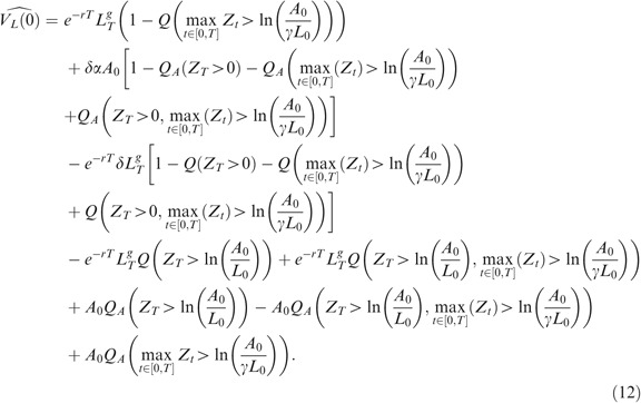
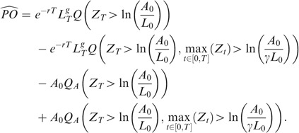
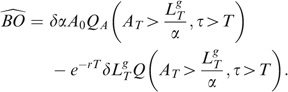
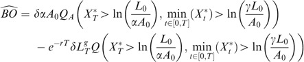
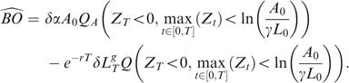
Defining ∀t X t *=X t −r g t, Z t =−X t *, Q A the A-neutral measure, and allowing for early default, the life insurance contract admits the following price:

Proof
-
This proof gives the closed-form development of (6) and (7) when the company's assets returns are modeled by a Lévy process of the Kou type.
Preliminary elements
The risk-neutral no-default condition on the company writes
or equivalently
thus, defining ∀t X t *=X t −r g t, the risk-neutral no-default condition writes
or
To conclude, with the convention b=ln(γL 0/A 0), one has
Computation of

 is defined by
One readily writes
which, from above, is equivalent to
now, setting ∀t Z t =−X t *, one can write
or finally
Computation of

Recall the definition
which can be straightforwardly rewritten as
or as
Using the previous lines of reasoning, one finally obtains
Computation of

From Eq. (7), one has
which becomes

or

We first compute
 , then
One readily has

Referring to the notations in the preliminaries
Defining ∀t Z t =−X t *, one can swap the min for a max according to
or
indeed, it will be more convenient to use
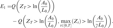
In order to compute E 2, we use the well-known change of numéraire technique. Choosing the assets A as the new numéraire, and denoting by Q A the associated measure (recall that Q A is such that (dQ A /dQ)F T =A T /A 0 e rT), we obtain

Then, obviously
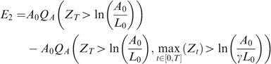
and finally
Computation of

From (7), we recall

We simplify this expression as

and then as
Introducing the return process X *, we obtain
or (noting in particular that L 0=αA 0)
Finally, it will be more convenient to use the following representation
which concludes the proof. □
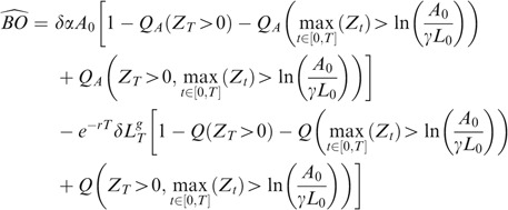
In order to compute Eq. (12), one needs to compute

and

and the joint term
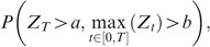
where the measure P will in fact be Q or Q A . The process A follows a Kou process under Q or Q A but of course with different parameters as shown in the previous section.


 is defined by


 , then


Remark
-
In case a fixed amount Λ of bankruptcy costs is incurred upon default, the payment to policyholders becomes A τ −Λ at time τ. The price of the product is therefore diminished by the amount
 . This amount can also be written as Λ∫0
T
e
−rτdQ(τ<x). It can be computed by performing a quadrature on Q(τ<.), which can be itself computed as the inverse Laplace transform of a known function (see Kou and Wang, 2003).
. This amount can also be written as Λ∫0
T
e
−rτdQ(τ<x). It can be computed by performing a quadrature on Q(τ<.), which can be itself computed as the inverse Laplace transform of a known function (see Kou and Wang, 2003).
 . This amount can also be written as Λ∫0
T
e
−rτdQ(τ<x). It can be computed by performing a quadrature on Q(τ<.), which can be itself computed as the inverse Laplace transform of a known function (see
. This amount can also be written as Λ∫0
T
e
−rτdQ(τ<x). It can be computed by performing a quadrature on Q(τ<.), which can be itself computed as the inverse Laplace transform of a known function (see Numerical analysis
The goal of this section is to give an overview of the effect of jump parameters on the contract value and on the choice of both the fair guaranteed rate and the fair participation rate.
Simulation data
We start by giving in Tables 1 and 2 the chosen parameter values. These values hold in all the sections, except otherwise indicated.
We recall that A 0 is the initial assets value and that σ is the volatility of the diffusive component of these assets. p is the probability of positive jumps w.r.t. negative ones: it is the probability that, given a jump occurred, this jump is positive. η 1 and η 2 are the parameters driving the exponential laws underlying the positive and negative jumps. One shows readily by integration that the average size of positive jumps is η 1 −1 while the average size of negative jumps is η 2 −1. λ is the jump intensity; it describes the arrival rate of jumps, independently of their size and sign (it just says how many jumps occur over a given time lag). So, the jumps of the considered process are fully described by the parameters p, η 1, η 2 and λ.
The parameter α is the leverage coefficient, r the unique constant interest rate prevailing on the market; r g is the guaranteed rate offered by the contract while δ is the participation coefficient. Finally T is the maturity, and γ is the default barrier multiplier used in the early default case.
Default at maturity
This part of the analysis is devoted to the simple case where default can only occur at the contract maturity.
In Figure 1 the contract value is graphed with respect to the jump process intensity. Each curve represents a different level of the diffusive component volatility. First, one can note the existence of optima: there are levels of jump intensity where the contract value is maximized. Then, comparing these graphs for different levels of σ, we remark that the optima are shifted to the left when σ increases: for a high value of σ, the optimum is for a small value of λ – when for a small value of σ, the optimum is for a high value of λ. This is not a surprise if one considers that λ and σ are two faces of the same coin. Indeed, the quadratic variation of the assets process, which is a description of its overall dispersion, is made of two components: one for the diffusion, one for the jumps. So this graph illustrates that the quadratic variation of the jumps is compensated by the quadratic variation of the diffusion. In other terms, when there is an important dispersion that is achieved through the diffusion (through σ), a small amount of additional dispersion coming from the jumps (so, from λ) is required in order to attain the optimum. The converse holds true. So, we observe in the default at maturity case, where the paths are by definition not important, an interesting compensation feature between diffusion and jump components.

Contract value w.r.t. λ for different levels of σ.
Figure 1 also shows that the contract value does not admit large variations, both in terms of λ (consider two values of a same curve, at different abscissas) and in terms of σ (consider two values of two different curves, but at the same abscissa). So, big variations of σ and λ imply small variations of the contract value. Then, in terms of parameter estimation, we refer the reader to the article of Aït-Sahalia (2004), which concentrates on the relative estimation of the continuous and discontinuous parts of the quadratic variation of a stochastic process. See also the recent paper of Aït-Sahalia and Jacod (2008), which gives a general test of the presence of jumps in a dynamics. To sum up, the impact of replacing erroneously λ by σ, or conversely, can have an impact on the kurtosis of the assets at the maturity, and can therefore induce a misprice of the contract. As appears from the previous observations, though, the contract's value is quite stable. As the coming subsection will show, the impact of mistaking jumps for diffusion can be a real concern in the case where default can happen early.
Figure 2, where σ is set at 10 percent, represents the curves linking r g and δ, the guaranteed and bonus rates given to the policyholders, for fair contracts (contracts whose initial book value is equal to their initial market value). These curves are computed for a given level of σ, given in the above table, but for varying levels of λ. On this graph, choose a given high level of r g : let λ increase, then for the contract to remain fair, δ should increase. This situation is the one when the contract is risky (in the sense of a possible default) and an increase in jump rate should be compensated by a higher participation of the insured. For a given, but now low value of r g , when λ increases, the participation coefficient of a fair contract decreases. In this situation, adding some jumps is not too risky in terms of probability of company bankruptcy: the increase in λ intervenes as an overall increase of the process quadratic variation, and the call-option effect dominates.

Participation level δ w.r.t. r g for different levels of λ (σ=0.1).
Figure 3 also plots curves linking the r g and δ of fair contracts, but for a σ set at 15 percent. We observe that in this situation, we nearly always have the monotonous situation where, for a given r g , an increase of λ corresponds to an increase of the participation level. In other terms, for a high degree of overall dispersion or risk, an increase in the jump intensity should be compensated economically by a higher participation rate granted to policyholders.

Participation level δ w.r.t. r g for different levels of λ (σ=0.15).
Finally, in Figure 4, we graph the fair participation level as a function of the leverage parameter α (assuming σ=0.1). Each curve corresponds to a different value of λ. In this example, the interpretations are straightforward. First of all, when λ is fixed, a higher initial leverage means that the insured provided a higher contribution to the initial liabilities of the company. Accordingly, they should obtain a higher proportion of the benefits. This proportion should obviously tend to one when α tends to one: in a company without stocks, the insured get back all the benefits. Then, because we set ourselves in a situation where the company is at risk due to jumps, an increase of λ, at a fixed level of α, means an increase of risk for the insured, and they should be compensated by an increase of their bonus rate.

Participation level δ w.r.t. α for different levels of λ (σ=0.1).
Figure 5 graphs the fair participation level as a function of the leverage parameter α, but for σ=0.15. We observe the same relationships as in Figure 4: for a fixed initial capital structure coefficient α, a higher intensity of jumps should be compensated by a higher participation coefficient δ. However, a comparison of the two figures shows that the participation coefficient δ is bigger for a higher level of σ, everything else kept equal. We also observe in the two figures, that for a fixed participation rate δ, a higher intensity induces a smaller α. This is a kind of compensation because a small α corresponds to a small initial input of capital in the company.

Participation level δ w.r.t. α for different levels of λ (σ=0.15).
Early default
We start by plotting, in Figure 6, the contract value as a function of the jump intensity λ, at different levels of σ. We remark that the same types of shapes emerge as when default could only occur at maturity. Indeed, optima with respect to the jump intensity exist, and these optima are increasing with the level of the volatility.

Contract value w.r.t. λ for different levels of σ.
One also observes that the optimal values of the contract are slightly higher in the early default case than in the default at maturity case. In fact, a continuously (or discretely but frequently) monitored company sees its value increased by the fact that very negative outcomes are made unlikely. In the case of default at maturity only, case of the previous subsection, the assets remaining upon default can be exceedingly small, whence a negative impact on firm valuation. One should insist though that in the presence of jumps, early default can mean a loss, because the assets not only touch but also cross the barrier – but this negative contribution to the contract value is less important than the negative contribution of a massive default at maturity.
Then, Figure 7 graphs the contract value with respect to the jump intensity, for various levels of the critical threshold γ. This graph is important because it shows the dependence of the contract price on the level of the early default barrier, when the assets are allowed to jump (we recall that the barrier is given by:  ). It clearly appears in the graph that the higher the barrier γ, the higher the contract value. Imposing a continuous surveillance where default is declared very easily, in other words when the barrier is high, is clearly beneficial to the contract value, so to policyholders. On the contrary, when γ becomes smaller, the control is less stringent: for γ tending to 0, we get back the limit case of a default occurring only at maturity. Ultimately, for an infinitesimal γ, we are therefore left with a curve similar to the ones from Figure 1.

Contract value w.r.t. λ for different levels of γ.
With Figure 8, we observe the dependence of the contract value on main parameters describing the jump component of the assets process: η 1 and η 2. We recall that η 1 −1 defines the average size of positive jumps when η 2 −1 gives the average size of negative ones. In Figure 8, we increase η 2 progressively and observe that for high levels of this parameter, so for negative jumps that become smaller and smaller on average, the contract is worth more. This makes sense because small negative jumps are less amenable to induce bankruptcy than big ones. Similar results hold (that we do not detail for the sake of brevity) when studying the impact of η 1. Indeed, a higher η 1 means smaller positive jumps, so jumps that bring the process less far from the default barrier, so a smaller contract value.

Contract value w.r.t. λ for different levels of η 2.
To conclude on jump parameters, we plot Figure 9 that represents the evolution of the contract value for various levels of the parameter p. We recall that p represents the probability that a jump, given it occurred, is positive. So a higher p means more positive jumps and less negative jumps. Not surprisingly, we observe that the contract value increases together with p, less negative jumps meaning a lower probability of getting bankrupt.

Contract value w.r.t. λ for different levels of p.
Then, to get an analytic pattern of the effects of early bankruptcy, we compute Table 3 that presents the values of the diverse sub-contracts involved. The volatility of the diffusive part of the assets is fixed at 0.1, and the intensity of the jumps is set to 0.1. We can readily perceive from the table that the early rebate  is a non-negligible component of the contract. When γ is high, equal to 80 percent, it represents more than 13 percent of the overall contract price. One should therefore not neglect the value of the continuous control of an insurance company. When γ becomes smaller, and not surprisingly, the relative importance of
  with regard to the contract value
  decreases to zero.
The preceding study emphasizes the importance of early bankruptcy. Let us conclude by now observing the effect of jumps. In Table 4 are displayed the same computations as in Table 3, but with only one parameter changing: the jump intensity is set to λ=0; said differently we come down to the Gaussian case without jumps. The same pattern as in Table 3 can be observed, but the values of and
and  are smaller. Our conclusion at this stage is that the introduction of jumps (symmetrical in our numerical example with η
1=η
2) increases the value of the early rebate; therefore continuous, or frequent in practice, control is even more desirable when the assets process admits a jump part, which is consistent with common intuition. For the sake of brevity, we do not include here the graphs representing δ as a function of r
g
or α for fair contracts, where patterns similar to the ones of Figures 2 and 4 are obtained.
are smaller. Our conclusion at this stage is that the introduction of jumps (symmetrical in our numerical example with η
1=η
2) increases the value of the early rebate; therefore continuous, or frequent in practice, control is even more desirable when the assets process admits a jump part, which is consistent with common intuition. For the sake of brevity, we do not include here the graphs representing δ as a function of r
g
or α for fair contracts, where patterns similar to the ones of Figures 2 and 4 are obtained.
We conclude this study by taking a look at the behavior of one of the contract components: the so-called default put option. Figure 10 represents the value of this option as a function of σ, and this for various levels of λ. The case λ=0 is interesting because it corresponds to the absence of jumps, so to the Gaussian model. We observe that in this case, the put option value remains null when the volatility is inferior to about 5 percent. Then, it increases as σ increases. For λ not null, we observe that the put option value is not null, also when σ=0. So, and not surprisingly, jumps can create bankruptcy by themselves. This figure is therefore interesting because it gives a price to the two contributions inducing bankruptcy: the jump (λ) and diffusion (σ) components of the assets process.

Put option value w.r.t. σ for different levels of λ.
Conclusion
In this article we study the valuation of participating life policies with guarantee. We give generic formulas that can prove to be very useful for subsequent research, especially quasi-closed formulas, in the third section. The originality of our approach is to consider a possible bankruptcy of the insurance company before contract maturity in a Lévy financial market framework. This problem has been analyzed in a Gaussian context and the results are well known. But there is now enough empirical evidence to admit that geometric Lévy processes can give good alternative to the classical geometric Brownian motion to model financial asset prices. The class of Lévy processes is actually very large. In option pricing many of them have been studied and in our context jump-diffusions with Gaussian jumps, Normal Inverse Gaussian, Generalized Hyperbolic Gamma and Meixner processes are among the more frequent choices. However, except for some jump-diffusion cases, no explicit formulas are available for European options, and numerical methods – especially Fast Fourier Transforms and partial integro-differential equation or Monte Carlo simulations – are needed. Dealing with exotic options is even more difficult and the pricing of barrier options is rather difficult.
We use the Kou process: a jump-diffusion with double exponential distributed jumps. These dynamics have already been used in the literature to tackle finance issues. For instance, Dao and Jeanblanc (2006) and Chen and Kou (2008) study the problem of the valuation of credit spreads, and Le Courtois and Quittard-Pinon (2006) the one of the prediction of default probabilities in such a context. With Kou processes, quasi-closed-form formulas are obtained for European options and an efficient procedure can be implemented for barrier options. It is what we use in our paper considering the bankruptcy in a so-called structural approach to default. We obtain a classical behavior in a fair value pricing for the couple participating level, guaranteed rate. Our modeling stresses the effects of early default on the life insurance contract considered here. First, to take into account early default is not innocuous, it really matters as it is illustrated in the previous section. Second, in our Lévy context we have shown that the impact of early default is more important than in the Gaussian environment. This framework could be used to analyze some equity linked contracts now sold in North America (for instance Equity-Indexed Annuities, see Hardy (2003) for a description). From a managerial standpoint this article shows the importance of efficient and frequent controls to make contracts safer.
Notes
This proof can be obtained using the Laplace exponent, while the original proof by Kou and Wang makes use of the Girsanov theorem. The former proof is available from the authors upon request.
References
Abramowitz, M. and Stegun, I.A. (1965) Handbook of Mathematical functions with formulas, graphs, and mathematical tables, Dover Publications.
Aït-Sahalia, Y. (2004) ‘Disentangling diffusion from jumps’, Journal of Financial Economics 74: 487–528.
Aït-Sahalia, Y. and Jacod, J. (2008) ‘Testing for jumps in a discretely observed process’, to appear in the Annals of Statistics.
Bacinello, A. (2001) ‘Fair pricing of life insurance participating policies with a minimum interest rate guaranteed’, Astin Bulletin 31 (2): 275–297.
Bacinello, A.R. (2003) ‘Fair valuation of a guaranteed life insurance participating contract embedding a surrender option’, The Journal of Risk and Insurance 70 (3): 461–487.
Ballotta, L. (2005) ‘A Lévy process-based framework for the fair valuation of participating life insurance contracts’, Special Issue of Insurance: Mathematics and Economics 37 (2): 173–196.
Ballotta, L., Haberman, S. and Wang, N. (2003) Modelling and valuation of guarantees in with-profit and unitised with-profit life insurance contracts, Actuarial Research Paper, 146, Cass Business School, London.
Ballotta, L., Haberman, S. and Wang, N. (2006) ‘The fair valuation problem of guaranteed annuity options: The stochastic mortality environment case’, Insurance: Mathematics and Economics 38 (1): 195–214.
Bernard, C., Le Courtois, O. and Quittard-Pinon, F. (2005) ‘Market value of life insurance contracts under stochastic interest rates and default risk’, Insurance: Mathematics and Economics 36 (3): 499–516.
Black, F. and Cox, J. (1976) ‘Valuing corporate securities: Some effects of bond indenture provisions’, Journal of Finance 31 (2): 351–367.
Bouchaud, J.-P. (2001) ‘Power laws in economics and finance’, Quantitative Finance 1: 105–112.
Brennan, M.J. and Schwartz, E.S. (1976) ‘The pricing of equity-linked life insurance policies with an asset value guarantee’, Journal of Financial Economics 3: 195–213.
Briys, E. and de Varenne, F. (1994) ‘Life insurance in a contingent claim framework: Pricing and regulatory implications’, The Geneva Papers on Risk and Insurance Theory 19 (1): 53–72.
Briys, E. and de Varenne, F. (1997) ‘On the risk of life insurance liabilities: Debunking some common pitfalls’, Journal of Risk and Insurance 64 (4): 673–694.
Briys, E. and de Varenne, F. (2001) Insurance from Underwriting to Derivatives, Wiley Finance, Chichester.
Brotherton-Ratcliffe, R. (1994) ‘Monte-Carlo monitoring’, Risk Magazine 7 (12): 53–57.
Carr, P., Geman, H., Madan, D.B. and Yor, M. (2002) ‘The fine structure of asset returns: An empirical investigation’, Journal of Business 75 (2): 305–332.
Chen, N. and Kou, S.G. (2008) ‘Credit spreads, optimal capital structure, and implied volatility with endogenous default and jump risk’, to appear in Mathematical Finance.
Cont, R. (2001) ‘Empirical properties of asset returns: Stylized facts and statistical issues’, Quantitative Finance 1 (2): 223–236.
Dao, T.B. and Jeanblanc, M. (2006) Double exponential jump diffusion process: A structural model of endogenous default barrier with roll-over debt structure, Working paper.
Fujiwara, T. and Miyahara, Y. (2003) ‘The minimal entropy martingale measures for geometric Lévy processes’, Finance and Stochastics 7: 509–531.
Grosen, A. and Jørgensen, P. (1997) ‘Valuation of early exercisable interest rate guarantees’, Journal of Risk and Insurance 64 (3): 481–503.
Grosen, A. and Jørgensen, P. (2002) ‘Life insurance liabilities at market value: An analysis of insolvency risk, bonus policy, and regulatory intervention rules in a barrier option framework’, Journal of Risk and Insurance 69 (1): 63–91.
Hardy, M. (2003) Investment Guarantees. Modeling and Risk Management for Equity-Linked Life Insurance, Wiley Finance, Hoboken.
Kassberger, S., Kiesel, R. and Liebmann, T. (2005) Fair valuation of insurance contracts under Lévy process specifications, Ulm University Working paper.
Kou, S.G. (2002) ‘A jump diffusion model for option pricing’, Management Science 48: 1086–1101.
Kou, S.G. and Wang, H. (2003) ‘First passage times of a jump diffusion process’, Advances in Applied Probability 35 (9): 504–531.
Kou, S.G. and Wang, H. (2004) ‘Option pricing under a double exponential jump diffusion model’, Management Science 50 (9): 1178–1192.
Le Courtois, O. and Quittard-Pinon, F. (2006) ‘Risk-neutral and actual default probabilities with an endogenous bankruptcy jump-diffusion model’, Asia-Pacific Financial Markets 13: 11–39.
Nielsen, J. and Sandmann, K. (1995) ‘Equity-linked life insurance: A model with stochastic interest rates’, Insurance: Mathematics and Economics 16: 225–253.
Ribeiro, C. and Webber, N.J. (2003) ‘Valuing path dependent options in the variance-gamma model by Monte Carlo with a gamma bridge’, Journal of Computational Finance 7 (2).
Ribeiro, C. and Webber, N.J. (2005) ‘Correcting for simulation bias in Monte Carlo methods to value exotic options in models driven by Lévy processes’, Applied Mathematical Finance.
Riesner, M. (2006) ‘Hedging life insurance contracts in a Lévy process financial market’, Insurance: Mathematics and Economics 38 (3): 599–608.
Tanskanen, A. and Lukkarinen, J. (2003) ‘Fair valuation of path-dependent participating life insurance contracts’, Insurance: Mathematics and Economics 33: 595–609.
Acknowledgements
The authors wish to thank Karim Aroussi, Georges de Nemeskeri-Kiss, Rivo Randrianarivony, and the two referees for their useful comments.
Author information
Authors and Affiliations
Appendix
Appendix
Computation of the function
The function is defined by:

where  z is a standard Brownian motion, N a Poisson process with intensity λ and Y has a double exponential law with parameters p, q, η
1, η
2. Kou (2002) develops in his Appendix B an algorithm to compute . We give here the main lines of this algorithm.
z is a standard Brownian motion, N a Poisson process with intensity λ and Y has a double exponential law with parameters p, q, η
1, η
2. Kou (2002) develops in his Appendix B an algorithm to compute . We give here the main lines of this algorithm.
With π n ≔P(N(T)=n)=e −λT(λT)n/n!, and I n defined below, we have the result

The expression Φ stands for the cdf of the standard normal law. P n , k and Q n, k are given by:

The functions I and Hh are linked as follows:

The function Hh (see Abramowitz and Stegun, 1965) can be obtained recursively:

with:

Rights and permissions
About this article
Cite this article
Le Courtois, O., Quittard-Pinon, F. Fair Valuation of Participating Life Insurance Contracts with Jump Risk. Geneva Risk Insur Rev 33, 106–136 (2008). https://doi.org/10.1057/grir.2008.11
Published:
Issue Date:
DOI: https://doi.org/10.1057/grir.2008.11