The effects of structural parameters on tangentially injected highly swirling turbulent tube air flow

Abstract

In the textile industry, air-jet nozzles known as Jetring, Nozzlering, Compact-jet and Siro-jet are used for the final spinning of the yarn. The air flow, which determines the yarn quality and other yarn properties, depends on the flow parameters such as pressure, mass flow rate, and the structural parameters of the air jet nozzle which acting on the flow parameters. In this study, SST turbulence model was selected and 225 kPa (absolute) total pressure was applied to the nozzle injectors. Approximately 2,500,000 tetrahedral elements are used for any geometry in the mesh prepared for parametric study. All parameters solved in ANSYS CFX 18.0 with used parametric study. The structural parameters were subjected to parametric CFD analysis and different flow parameters such as mass flow, swirling number, geometric swirling number, Reynolds number, vorticity, helicity real eigen, velocity, velocity w (z-axis velocity, i.e. twisting chamber axis), total pressure, flow pressure were compared.

1 Introduction

There are swirling flows in many areas of our lives and engineering. “Swirling flow” [1] is defined as the rotating helical flow. For example, in nature events: tornadoes, hurricanes, water vents, etc. many events can be shown. However, in the field of engineering, cyclone separators and jet engines, as well as swirling flows in many areas are encountered. In combustion systems such as gas turbine engines, diesel engines, industrial burners and boilers, helical rotating flows are used to improve and control the mixing ratio between fuel and oxygen streams to achieve flame geometries and heat release rates appropriate to particular process applications [2]. An important feature of rotating flows has been proposed by Ranque Hilsch [3]. He discovered the ability of vortex tubes to separate compressed air into the hot and cold air streams located near the periphery of the periphery of the tube. The Ranque-Hilsch vortex tube has been used in a number of engineering applications using this flow behavior, such as separation of different molecular weight gases, cooling arrangement, cyclone separation, gas turbine cyclone, combustion chamber and spray driers [4]. An example of the swirling flows is the air-jet nozzles used in the textile industry on spinning machines. Swirling air flow is produced in air nozzle depending on nozzle geometry and compressed air [5, 6]. The helical rotating flow in turbulent jets results in an increase in jet growth, drift speed and decay rate of the jet. These effects also increase when helical rotation density increases [4]. Swirling flows depend on different parameters. Most of these parameters were formulated and found as a result of studies. The most important of these is the Number of Swirling (Sn). The integral definition of the swirling number is expressed as the ratio of the axial flux of the angular momentum to the axial momentum flux and radius multiplication [1, 7, 8].

$$S_{n} = \frac{Angular \,Momentum}{R \cdot Axial \,Momentum} = \frac{{G_{Ang} }}{{RG_{Ax} }} = \frac{{\mathop \smallint \nolimits_{0}^{2\pi } \mathop \smallint \nolimits_{0}^{R} u_{z} u_{\phi } r^{2} drd\phi }}{{R\mathop \smallint \nolimits_{0}^{2\pi } \mathop \smallint \nolimits_{0}^{R} u_{z}^{2} rdrd\phi }}$$

(1)

where ${\text{R}}$ twisting chamber radius, $u_{z}$ axial velocity component, $u_{\phi }$ tangential velocity component, $r$ and $\phi$ radial and angular coordinates taken according to the main hole (twisting chamber) center. Since these values cannot be known in advance, a geometric swirling number (Sg) can also be defined based on the ratio of mass flows in the twisting chamber and in the entrance cross-sectional areas. These values can also be defined in a geometric swirling number (Sg) based on the ratio of mass flows in the twisting chamber and in the air inlet entrance (injectors) cross-sectional areas as it is not previously known before the CFD (computational fluid dynamics) analysis or experimental studies are performed [1, 9, 10].

$$S_{g} = \left( {\frac{{m_{t} }}{{m_{T} }}} \right)^{2} \left( {\frac{{D_{tc} }}{d}} \right)^{2} \frac{sin\theta }{N}$$

(2)

where $m_{t}$ and $m_{T}$ mass flow in the injectors (total) and in the test section (twisting chamber). According to Eq. 2, geometric swirling number (i.e. the swirl density) is dependent on the diameter of the twist chamber $D_{tc}$, injector diameter $d$, injector angle $\theta$, and the number of injectors $N$ [1, 10].

The calculation of the turbulent helical rotating flow by computational fluid dynamics is the determining factor for the appropriate turbulence model. The swirling number is a decisive factor for the turbulence model of turbulent helical rotating flow in the analysis of computational fluid dynamics. Chen et al. [11] reported that, determined a weak swirling flow at swirling number of 0.03, moderate swirling flow at swirling number of 0.26, highly swirling flow at swirling number of 0.8. Parra-Santos et al. [12] reported that, determined a weak swirling flow at swirling number of 0.2, moderate swirling flow at swirling number of 0.7, highly swirling flow at swirling number of 1.2. In literature, it is suggested that if the number of swirling is less than 0.5 there is a weak or medium swirling flow, it can be sufficient flow analysis and the k-ε turbulence model can be used (with realizable k–ε, RNG k–ε selections). If the swirling number is greater than 0.5, it is emphasized that it has high swirling flow and Reynolds Stress Models should be preferred [13]. Guo [8] reported that the Reynolds Stress Model (RSM) is generally more reliable than two-equation models, but the RSM model needs large memory and processor time, and convergence is more difficult. As an alternative, the realizable k–ε turbulence model closes the turbulent Navier–Stokes equations. The realizable k–ε model is a revised k–ε turbulence model. Compared to the standard k–ε turbulence model, the realizable k–ε model exhibits superior performance for flows involving boundary layers, flow separations, and rotation under strong reverse pressure gradients. In another turbulent swirling flow study, turbulence models were compared under steady flow analysis and SST (Shear Stress Transport) turbulence model was found to be closest to experimental study. According to study, The SST model provides the transition between the potential flow and the boundary layer flow in a suitable way thanks to the first blending function, In the second blending function, it is seen that both the sensitivity to the flow under the reverse pressure and the accuracy of the result in the regions where flow separations are present, and it has been found to be successful in modeling the existing turbulence in the problem [14].

1.1 Used CFD turbulence model

The two-equation turbulence models are widely used because of a good balance between numerical effort and calculation accuracy. Two equation models are more complex than zero equation models [15]. Velocity and length scales are solved using separate transport equations. Therefore, it is called the two equation model.

In two equation models for example k–ω, k–ε, realizable k–ε, RNG k–ε, etc., the turbulence rate scale is calculated according to the turbulence kinetic energies resulting from the dissolution of transport equations. The turbulence length scale is generally estimated by turbulence kinetic energy and diffusion rate, which are two characteristics of the turbulent area. The turbulence kinetic energy diffusion ratio provides the solution of the transport equation.

There are also models of turbulence that combine the advantageous aspects of two equation models such as baseline (BSL) and shear stress transport (SST). The BSL model combines the advantageous parts of the Wilcox k–ω [16] and k–ε models. But it still fails to estimate the beginning and amount of separation of flow on smooth surfaces. This lack of reasons are given in detail by Menter [17]. The main reason for the low sensitivity of the results is that it cannot solve the turbulent shear stress transport model. These results are estimated from the eddy viscosity that has been achieved. The k–ω based SST model, as in the BSL model, combines the advantageous parts of the k–ω and k–ε models, giving very accurate predictions in the flow states that are separated under the reverse pressure gradients from the start of the flow [14].

The SST includes a collation function to add a cross-diffusion term in the ${{\upomega }}$ equation in the turbulence model and to ensure that the model equations behave appropriately in both the near-wall and far area regions [18].

1.1.1 SST turbulence model transport equations

SST turbulence model basically has the same definition as k–ω model [18,19,20,21]:

$$\frac{\partial }{\partial t}\left( {\rho k} \right) + \frac{\partial }{{\partial x_{i} }}\left( {\rho ku_{i} } \right) = \frac{\partial }{{\partial x_{j} }}\left( {{{\varGamma }}k\frac{\partial k}{{\partial x_{j} }}} \right) + G_{k} - Y_{k} + S_{k}$$

(3)

and

$$\frac{\partial }{\partial t}\left( {\rho \omega } \right) + \frac{\partial }{{\partial x_{i} }}\left( {\rho \omega u_{i} } \right) = \frac{\partial }{{\partial x_{j} }}\left( {{{\varGamma }}\omega \frac{\partial \omega }{{\partial x_{j} }}} \right) + G_{\omega } - Y_{\omega } + D_{\omega } + S_{\omega }$$

(4)

where G_k is the production of turbulence kinetic energy because of average velocity gradients. G_ω is the production of ω. Γ_k and Γ_ω is the effective diffusivity of k and ω. Y_k and Y_ω is the dissipation of k and ω owing to turbulence. D_ω is the cross diffusion term formulized in Eq. 21. S_k and S_ω are user-defined resource terms [18,19,20,21,22,23,24,25,26].

1.1.2 Effective diffusivity model

SST k–ω model effective diffusivities are given by [18, 20, 27]:

$${{\varGamma }}_{{k = \mu + \frac{{\mu_{t} }}{{\sigma_{k} }}}}$$

(5)

$${{\varGamma }}_{{\omega = \mu + \frac{{\mu_{t} }}{{\sigma_{\omega } }}}}$$

(6)

where σ_k and σ_ω are the turbulent Prandtl numbers for k and ω. The turbulent viscosity, µt, is calculated as follows [18, 20]:

$$\mu_{t} = \frac{\rho k}{\omega }\frac{1}{{max\left[ {\frac{1}{{\alpha^{*} }},\frac{{{{\varOmega }}F_{2} }}{{a_{1\omega } }}} \right]}}$$

(7)

where

$${{\varOmega }} \equiv \sqrt {2{{\varOmega }}_{ij} {{\varOmega }}_{ij} }$$

(8)

$$\sigma_{k} = \frac{1}{{\frac{{F_{1} }}{{\sigma_{k,1} }} + \frac{{1 - F_{1} }}{{\sigma_{k,2} }}}}$$

(9)

$$\sigma_{\omega } = \frac{1}{{\frac{{F_{1} }}{{\sigma_{\omega ,1} }} + \frac{{1 - F_{1} }}{{\sigma_{\omega ,2} }}}}$$

(10)

Because of low Reynolds number correction, α* damps the turbulent viscosity α* computed as follows [18]:

$$a^{*} = a_{\infty }^{*} \left( {\frac{{a_{\infty }^{*} + Re_{t} /Re_{k} }}{{1 + Re_{t} /Re_{k} }}} \right)$$

(11)

where

$$Re_{t} = \frac{\rho k}{\mu \omega }$$

(12)

$$R_{k} = 6$$

(13)

$$a_{0}^{*} = \frac{{\beta_{i} }}{3}$$

(14)

$$\beta_{i} = 0.072$$

(15)

For the high Reynolds number form of the k–ω model, $\varvec{a}^{\varvec{*}}$ = $\varvec{a}_{\infty }^{\varvec{*}}$ = 1. Ω_ij is the average rate of rotation tensor and the blending functions, F₁ and F₂, are given by [18, 22, 23]:

$$F_{1} = \tanh \left( {\Phi_{1}^{4} } \right)$$

(16)

$${{\Phi }}_{1} = min\left[ {max\left( {\frac{\sqrt k }{0.09\omega y},\frac{500\mu }{{\rho y^{2} \omega }}} \right),\frac{4\rho k}{{\sigma_{\omega ,2} D_{\omega }^{ + } y^{2} }}} \right]$$

(17)

$$D_{\omega }^{ + } = max\left[ {2\rho \frac{1}{{\sigma_{\omega ,2} }}\frac{1}{\omega }\frac{\partial k}{{\partial x_{j} }}\frac{\partial \omega }{{\partial x_{j} }},10^{ - 20} } \right]$$

(18)

$$F_{2} = \tanh \left( {\Phi_{2}^{2} } \right)$$

(19)

$${{\Phi }}_{2} = max\left[ {2\frac{\sqrt k }{0.09\omega y},\frac{500\mu }{{\rho y^{2} \omega }}} \right]$$

(20)

where $D_{\omega }^{ + }$ is the positive parts of the cross-diffusion term and $y$ is the distance to the next face. SST model is based on both the standard k–ω model and the standard k–ε model. Blends these two turbulence model together, the standard k–ε model has been transformed into equations based on k and ω, which leads to the intake of a cross-diffusion term (D_ω in Eq. 4). D_ω is defined as [18,19,20, 22, 23, 28, 29]:

$$D_{\omega } = 2\left( {1 - F_{1} } \right)\rho \sigma_{\omega ,2} \frac{1}{\omega }\frac{\partial k}{{\partial x_{j} }}\frac{\partial \omega }{{\partial x_{j} }}$$

(21)

1.1.3 Model constants

$$\sigma_{k,1} = 1.176$$

(22)

$$\sigma_{\omega ,1} = 2.0$$

(23)

$$\sigma_{k,2} = 1.0$$

(24)

$$\sigma_{\omega ,2} = 1.168$$

(25)

$$a_{1} = 0.31$$

(26)

$$\beta_{i,1} = 0.075$$

(27)

$$\beta_{i,2} = 0.0828$$

(28)

All the other model constants ($\alpha_{\infty }^{*} ,\alpha_{\infty } ,\alpha_{0} ,\beta_{\infty }^{*} ,R_{\beta } ,R_{k} ,R_{\omega } ,\xi^{*}$ and $M_{t0}$) have the equal values as the standard k-ω model [18].

2 Computational method

The first design for the idea of obtaining fibers by collecting and twisting fibers using a rotating fluid was developed by Götzfried [30]. Götzfried [30] and then Pacholski et al. [31, 32] showed that the air jets entering the tangentially into the nozzle hole caused the vortex in the nozzle and could be twisted to the yarn passing through the center of the rotating air stream at high speeds [33]. In recent years, the development of modified spinning systems with the addition of air nozzles to various spinning systems and research on the effect of these systems on yarn properties are being studied. These systems, which are developed depending on the spinning system where air is used, are named with Jetring, NozzleRing, Compact-jet [5, 34] and Siro-jet [5, 33, 35,36,37]. Figure 1 shows an air jet nozzle mounted on the Siro-jetsystem. An air jet nozzle mounted on the Siro-jetsystem is shown in Fig. 1.

Fig. 1

Application of an air nozzle on the sirospun spinning system (siro-jet)

Yilmaz [36] Evaluates the effect of pseudo-twist on the yarn properties of compressed air fed into the air ring in the conventional ring spinning system. In order to determine the performance of the core, the yarns produced in the Ne 30/1 yarn number can represent the linear density. In this study, the air nozzle in the conventional ring spinning systems produced using yarns Similarly to literature “Jetring yarn” was called.

Jetring, Compact-jet and Siro-jet spinning systems consist of three basic components: compressed air, nozzle and yarn. Compressed air with a certain value from the compressor is transported to the level and passed through the thread. The nozzle has a very simple structure and consists of a nozzle housing and nozzle body (Fig. 2). The nozzle body part has a circular cross-section consisting of the main hole (twisting chamber) (1), injectors (2), connecting screw for the nozzle housing (3) and the nozzle outlet (4) (Fig. 2b). The main hole extends from the nozzle entrance to the nozzle outlet. The injectors are positioned so as to be tangential to the twisting chamber. The nozzle housing conveys the compressed air from the compressor to the twisting chamber section of the device via the injectors [35, 36].

Fig. 2

Nozzle housing (a), nozzle body (b) and nozzle assembly (c)

Yilmaz [36] was determined that there was not a single type of flat hair with the lowest hairiness values. It has been determined that the rate of improvement in hairiness values has changed depending on the structural parameters and air pressure value. However, it was found that the different yarn types were effective on other yarn properties which determine the yarn quality as well as yarn hairiness.

2.1 Parametric study

Nozzle geometry for parametric study the flow volume with the Ansys Design Modeller 18.0 program drawed as parameter dependent. The representation of the drawing of flow volume, parameters and boundary conditions are given in Fig. 3. According to these ranges mentioned in Table 1; 5 different auxiliary hole angle × 3 different main hole diameter × 5 different auxiliary hole diameter × 2 different environmental auxiliary hole number = total 150 different geometry modelled.

Fig. 3

3D model draw of a nozzle flow volume with 3 injectors

Table 1 Parametric study review interval

A parametric working table (Table 1) was created on Ansys Workbench 18.0 by selecting the desired measurements. According to Table 1, 150 different geometry configurations according to the 3 injectors 75 and 4 injectors 75 divided into 2 groups. ANSYS Workbench 18.0 parametric working table created by defining 225 kPa pressure of 75 different geometries of 3 injectors is given in Table 2.

Table 2 Parametric study plan

Approximately 2,500,000 tetrahedral elements are used for any geometry in the mesh prepared for parametric study (Number of elements varies according to structural parameters). With the ICEM CFD mesher in ANSYS CFX 18.0, the body of influence and the a thin mesh of size 0.07 mm element were assigned to the cylindrical control volume which is 1 mm before and 2 mm after the distance the injectors are opened to the twisting chamber. For the twisting room boundary layer, the size of the element is 0.1 mm face sizing was assigned. The detail view of the mesh topology is given in Fig. 4.

Fig. 4

Mesh detail of a nozzle with 3 injectors generated with ANSYS ICEM CFD mesher

After the parameters and mesh topology are determined, in ANSYS CFX 18.0 software as shown in Fig. 3, the inlet boundary condition is defined as 225 kPa total pressure from the air inlet. The relative pressure value is defined as “0” by selecting static pressure in the outlet boundary condition. Opening boundary condition defined in fiber inlet boundary condition and as in outlet boundary condition the relative pressure value is defined as “0”. Air at 25° is selected as fluid and reference pressure defined as 101,325 kPa. All parametric study configurations were solved separately using the SST turbulence model.

2.2 CFD verification

CFD Verification is based on mass flow measurement and comparison. The mass flow rate measurements of the air inlets which have been fed to the nozzle injectors and the air outlets which leaving the nozzle bending chamber were carried out by Alicat Scientific Brand M series mass flow meters (Fig. 5). Gas mass flow meters from Alicat are highly flexible instruments that can be used with many gases across a very wide range. Measure mass flow, volumetric flow, pressure and temperature in a compact device. The M series is suitable for most flow measurement applications, with models that can measure flow rates as high as 0.083 m³/s or as low as 4.16 × 10⁻⁸ kg/s. Alicat mass flow meter accuracy is 0.8% of the reading (0.4% optional) + 0.2% full-scale repeatability. CFD validation was performed by means of air inlet and outlet mass flow measurements with an experimental study and compared with CFD results. Air inlet comparison data are given in Fig. 7 and outlet comparison data are given in Fig. 9.

Fig. 5

Measuring with Alicat Scientific Brand M series mass flow meter

3 Results and discussion

As shown in Fig. 3, the nozzle of 27 mm length is divided into planes with 1 mm spacing along the z axis (twisting chamber axis). The place where the injectors are connected to the twisting chamber of the nozzle is 4 mm ahead of the fiber inlet. The representation of the defined plans on the nozzle is shown in Fig. 6.

Fig. 6

View of the reference plane of a nozzle with 3 injectors

3.1 Comparison of mass flow

According to the mass flow graph of the air inlet in Fig. 7, when the number of circular injectors, injector diameter, injector angle and twisting chamber diameter values increases, the air inlet mass flow enters into the nozzle also increases. The highest structural configuration of the air inlet upstream mass flow rate is given in Table 3, while the lowest 5 structural configurations are given in Table 4.

Fig. 7

Air inlet mass flow comparison chart

Table 3 The highest 5 nozzle configuration for air inlet mass flow rate according to the CFD results under 225 kPa air pressure

Table 4 The lowest 5 nozzle configuration for air inlet mass flow rate according to the CFD results under 225 kPa air pressure

According to the fiber inlet mass flow graph given in Fig. 8, the negative flow rate of some nozzle configurations means that the amount of air exiting is more dominant than the intake on the fiber inlet boundary layer. It is desirable to have only air intake from the fiber inlet opening to give a smooth twist to the fiber where placed in the middle of this swirling nozzle. Having an air outlet out of the fiber inlet opening disrupts the flow of an optimum swirling and thus adversely affects the twist of the fibers on the fiber. Exiting the air out of the fiber inlet boundary layer an optimum swirling disrupts the flow and thus adversely affects the twist of the fibers on the fiber. In this case, it is thought that it will affect the yarn quality (hairiness, strength, yarn smoothness etc.) negatively.

Fig. 8

Fiber inlet mass flow comparison chart

As seen in Fig. 8, in most of the configurations where the diameter of the twisting chamber is Ø2 mm (DP 1–DP 25), it is understood from the graph an outward air outlet occurs from the fiber inlet boundary layer. According to this case is not recommended to use Ø2 mm twisting chamber diameter nozzle. According to the mass flow graph of the air inlet in Fig. 8, when the injector diameter values increases, the fiber inlet mass flow rate enters into the nozzle decreases. On the contrary the increase in the twisting chamber diameter and the injector angle increases the fiber inlet mass flow rate enters into the nozzle. In the same structural configuration, the number of circular injectors has no significant effect on the fiber inlet mass flow rate of the change. The structural configuration of 5 different nozzles with the highest value of the fiber inlet mass flow rate is given in Table 5, while the 5 lowest nozzle structural configurations are given in Table 6.

Table 5 The highest 5 nozzle configuration for fiber inlet mass flow rate according to the CFD results under 225 kPa air pressure

Table 6 The lowest 5 nozzle configuration for fiber inlet mass flow rate according to the CFD results under 225 kPa air pressure

According to the outlet mass flow graph given in Fig. 9, the reason for the negative value of the mass flow rate is that the air outlet direction is from the nozzle to the outside environment. As can be seen from the graph in Fig. 9, the increase of the injector diameter reduces the mass flow, and the increase in the twisting chamber diameter and the injector angle increases the outlet boundary layer mass flow (in the negative direction). In the same structural configuration, the number of circular injectors has no significant effect on the outlet boundary layer mass flow of the change. The structural configuration of 5 different nozzles with the highest value (in the negative direction) of the outlet inlet mass flow rate is given in Table 7, while the 5 lowest nozzle structural configurations are given in Table 8.

Fig. 9

Outlet inlet mass flow comparison chart

Table 7 The highest 5 nozzle configuration for outlet mass flow rate according to the CFD results under 225 kPa air pressure

Table 8 The lowest 5 nozzle configuration for outlet mass flow rate according to the CFD results under 225 kPa air pressure

3.2 Comparison of swirling number and geometric swirling number

According to the number of geometric swirling number (Sg) graph given in Fig. 10, when the injector diameter, number of circular injectors and injector angle values increases, the geometric swirling number value decreases. On the contrary the increase in the twisting chamber diameter increases geometric swirling number value. The structural configuration of 5 different nozzles with the highest value the geometric swirling number is given in Table 9, while the 5 lowest nozzle structural configurations are given in Table 10. According to the studies in the literature [11,12,13] all of the parametric studies performed in this study are accepted as highly swirl.

Fig. 10

Geometric swirling number (Sg) comparison chart

Table 9 The highist 5 nozzle configuration for geometric swirling number (Sg) according to the CFD results under 225 kPa air pressure

Table 10 The lowest 5 nozzle configuration for geometric swirling number (Sg) according to the CFD results under 225 kPa air pressure

According to the geometric swirling number (Sn) graph in Fig. 11, when the injector diameter, number of circular injectors and injector angle values increases, the swirling number value decreases. On the contrary the increase in the twisting chamber diameter increases swirling number value.

Fig. 11

Swirling number (Sn) comparison chart at plane 4 mm

Although the number of geometric swirling increases as the injector angle increases, according to the geometric swirling number formula (Eq. 2), but the reason for the decrease in the graph shown in Fig. 11 is based on the angle to the vertical instead of the horizontal angle as the injector angle (Fig. 3). But still, the geometric swirling number was calculated by taking into account the horizontal angle as in the literature [1]. The structural configuration of 5 different nozzles with the highest value the swirling number is given in Table 11, while the 5 lowest nozzle structural configurations are given in Table 12 where the injectors are opened to the twisting chamber (plane 4 mm).

Table 11 The highist 5 nozzle configuration for swirling number (Sn) according to the CFD results under 225 kPa air pressure (where injectors are opened to the twisting chamber, 4 mm ahead of the fiber inlet)

Table 12 The lowest 5 nozzle configuration for swirling number (Sn) according to the CFD results under 225 kPa air pressure (where injectors are opened to the twisting chamber, 4 mm ahead of the fiber inlet)

A comparative graph of the swirling number (Sn) and the geometric swirling number (Sg) is given in Fig. 12. According to this graph, it is seen that Sn and Sg values tend to be in a coherent and correct ratio. The number of geometric swirling can be used to estimate the swirling density before the CFD analysis, since the momentum values mentioned in the swirling number formula (Eq. 1) cannot be pre-specified.

Fig. 12

Swirling number (Sn) at plane 4 mm—geometric swirling number (Sg)—comparison chart

According to the results, swirl number or geometric swirl number, injector diameter and injector angle values tend to decrease with increasing. On the contrary, as the diameter of the twist chamber increases, the number of swirl decreases.

3.3 Comparison of total pressure and flow pressure

According to the total pressure graph given in Fig. 13, when the twisting chamber diameter and injector angle values increases, the total pressure value decreases. On the contrary increase the injector diameter, increases total pressure value. In the same structural configuration, the number of circular injectors has no significant effect on the total pressure value of the change. The structural configuration of 5 different nozzles with the highest total pressure values is given in Table 13, while the 5 lowest nozzle structural configurations are given in Table 14 where the injectors are opened to the twisting chamber (plane 4 mm).

Fig. 13

Total pressure comparison chart at plane 4 mm

Table 13 The highist 5 nozzle configuration for total pressure value according to the CFD results under 225 kPa air pressure (where injectors are opened to the twisting chamber, 4 mm ahead of the fiber inlet)

Table 14 The lowest 5 nozzle configuration for total pressure value according to the CFD results under 225 kPa air pressure (where injectors are opened to the twisting chamber, 4 mm ahead of the fiber inlet)

According to the flow pressure graph given in Fig. 14, when the twisting chamber diameter increases, the flow pressure value decreases. On the contrary increase the injector diameter, injector angle and the number of circular injectors, increases total pressure value. The structural configuration of 5 different nozzles with the highest flow pressure values is given in Table 15, while the 5 lowest nozzle structural configurations are given in Table 16 where the injectors are opened to the twisting chamber (plane 4 mm).

Fig. 14

Flow pressure comparison chart at plane 4 mm

Table 15 The highist 5 nozzle configuration for flow pressure value according to the CFD results under 225 kPa air pressure (where injectors are opened to the twisting chamber, 4 mm ahead of the fiber inlet)

Table 16 The lowest 5 nozzle configuration for flow pressure value according to the CFD results under 225 kPa air pressure (where injectors are opened to the twisting chamber, 4 mm ahead of the fiber inlet)

As the injector angle and the twist chamber diameter increase, the total pressure decreases. On the contrary, increasing the diameter of the injector increases the total pressure value. There is a different improvement in flow pressure value. Increasing the injector diameter and injector angle increases the flow pressure value. On the contrary, the increase of the bending chamber diameter decreases the flow pressure value. Flow pressure value is one of the major features to give the yarn twist. It is therefore desirable that the twist chamber diameter is low.

3.4 Comparison of Reynolds number

According to the Reynolds number graph given in Fig. 15, when the twisting chamber diameter and injector angle values increases, the Reynolds number value decreases. On the contrary increase the injector diameter, increases Reynolds number value. In the same structural configuration, the number of circular injectors has no significant effect on the Reynolds number value of the change. The structural configuration of 5 different nozzles with the highest Reynolds number values is given in Table 17, while the 5 lowest nozzle structural configurations are given in Table 18 where the injectors are opened to the twisting chamber (plane 4 mm).

Fig. 15

Reynolds number comparison chart at plane 4 mm

Table 17 The highest 5 nozzle configuration for Reynolds number value according to the CFD results under 225 kPa air pressure (where injectors are opened to the twisting chamber, 4 mm ahead of the fiber inlet)

Table 18 The lowest 5 nozzle configuration for Reynolds number value according to the CFD results under 225 kPa air pressure (where injectors are opened to the twisting chamber, 4 mm ahead of the fiber inlet)

Increasing the injector diameter increases the Reynolds number and increasing the injector angle decreases it. When CFD results are examined, it is understood that the twist chamber diameter change has no significant effect on Reynolds number. It is undesirable to increase this number since the rise of the Reynolds number will make the swirling flow even more unstable. These values must therefore be taken into account when testing the yarn. According to the Reynolds number graph, it is recommended to test nozzles with Ø0.5 mm injector diameter and 35°–40° injector angle range which give low results.

3.5 Comparison of velocity and velocity w

According to the velocity graph given in Fig. 16, when the twisting chamber diameter values increases, the velocity value decreases. On the contrary increase the injector diameter, increases velocity value. In the same structural configuration, the number of circular injectors and injector angle has no significant effect on the velocity value of the change. The structural configuration of 5 different nozzles with the highest velocity values is given in Table 19, while the 5 lowest nozzle structural configurations are given in Table 20 where the injectors are opened to the twisting chamber (plane 4 mm). In plane 4 mm, the structural configuration of the nozzle where the velocity is highest: Twist chamber diameter Ø2 mm, injector diameter Ø0.9 mm, injector angle 25° and have 3 injector. Airflow velocity is calculated as 390.3 m/s (1.14 Mach). The structural configuration of the lowest speed nozzle is: Twist chamber diameter Ø3 mm, injector diameter Ø0.5 mm, injector angle 25° and have 4 injector. Airflow velocity is calculated as 192.7 m/s (0.56 Mach).

Fig. 16

Velocity comparison chart at plane 4 mm

Table 19 The highest 5 nozzle configuration for velocity value according to the CFD results under 225 kPa air pressure (where injectors are opened to the twisting chamber, 4 mm ahead of the fiber inlet)

Table 20 The lowest 5 nozzle configuration for velocity value according to the CFD results under 225 kPa air pressure (where injectors are opened to the twisting chamber, 4 mm ahead of the fiber inlet)

According to the velocity w (velocity in z axis) graph given in Fig. 17, when the twisting chamber diameter values increases, the velocity w value decreases. On the contrary increase the injector diameter and injector angle, increases velocity w value. In the same structural configuration, the number of circular injectors has no significant effect on the velocity value of the change. The structural configuration of 5 different nozzles with the highest velocity w values is given in Table 21, while the 5 lowest nozzle structural configurations are given in Table 22 where the injectors are opened to the twisting chamber (plane 4 mm).

Fig. 17

Velocity w comparison chart at plane 4 mm

Table 21 The highest 5 nozzle configuration for velocity w value according to the CFD results under 225 kPa air pressure (where injectors are opened to the twisting chamber, 4 mm ahead of the fiber inlet)

Table 22 The lowest 5 nozzle configuration for velocity w value according to the CFD results under 225 kPa air pressure (where injectors are opened to the twisting chamber, 4 mm ahead of the fiber inlet)

3.6 Comparison of vorticity

According to the vorticity graph given in Fig. 18, when the twisting chamber diameter increases, the vorticity (curl of velocity) value decreases. In the same structural configuration, the number of circular injectors, the injector diameter and injector angle has no significant effect on the vorticity value of the change. The structural configuration of 5 different nozzles with the highest vorticity values is given in Table 23, while the 5 lowest nozzle structural configurations are given in Table 24 where the injectors are opened to the twisting chamber (plane 4 mm).

Fig. 18

Vorticity comparison chart at plane 4 mm

Table 23 The highest 5 nozzle configuration for vorticity value according to the CFD results under 225 kPa air pressure (where injectors are opened to the twisting chamber, 4 mm ahead of the fiber inlet)

Table 24 The lowest 5 nozzle configuration for vorticity value according to the CFD results under 225 kPa air pressure (where injectors are opened to the twisting chamber, 4 mm ahead of the fiber inlet)

Vorticity, also known as curl of velocity, is one of the most important values for swirling nozzles. The success parameter of the swirling nozzle is directly proportional to the high vorticity. When performing yarn tests, nozzles with high vorticity should be considered in order to obtain more successful results. Therefore, for yarn tests, it is estimated that nozzles with a twist chamber diameter of Ø2 mm will give better results than nozzles with a larger twist chamber diameter. It is seen that there is an inverse ratio with the vorticity value and swirling number. It is understood from the graph that the number of swiling is minimum in nozzle configurations with maximum vorticity.

3.7 Comparison of helicity

According to the helicity real eigen graph given in Fig. 19, when the twisting chamber diameter values increases, the helicity real eigen value decreases. On the contrary increase the injector diameter, the number of circular injectors and injector angle, increases helicity real eigen value. The structural configuration of 5 different nozzles with the highest helicity real eigen values is given in Table 25, while the 5 lowest nozzle structural configurations are given in Table 26 where the injectors are opened to the twisting chamber (plane 4 mm).

Fig. 19

Helicity comparison chart at plane 4 mm

Table 25 The highest 5 nozzle configuration for helicity value according to the CFD results under 225 kPa air pressure (where injectors are opened to the twisting chamber, 4 mm ahead of the fiber inlet)

Table 26 The lowest 5 nozzle configuration for helicity value according to the CFD results under 225 kPa air pressure (where injectors are opened to the twisting chamber, 4 mm ahead of the fiber inlet)

Helicity real eigen value shows the same tendencies as vorticity value. This result was already foreseen. The reason for this is that the value of helicality and vorticity are mathematically based on similar mathematical formulation.

4 Conclusions

Table 27 shows the results of the computational fluid dynamics analysis result parameters when the values of the nozzle structural parameters are increased. In this way, it is understood that for each result parameter which structural parameter has a positive or negative effect on the result. If the (+) sign indicates an increase in value, (−) indicates a decrease in value. The sign (o) indicates that the value does not change significantly.

Table 27 Effects of change of nozzle structural parameters on CFD analysis result parameters

• Compared to the air flow mass flow graph given in Fig. 7, the geometric swirling number in Fig. 10 and the swirling number in Fig. 11, geometric swirling number and swirling number are at maximum value in structural configuration where air inlet mass flow is minimum and an inverse ratio between them appears.

• The only parameter that increases swirling number and geometric swirling number is the increase in the diameter of the twisting chamber. The positive change in other structural parameters decreases swirling number and geometric swirling number.

• According to this Sg–Sn comparison graph (Fig. 12), it is seen that Sn and Sg values tend to be in a coherent and correct ratio. The number of geometric swirling can be used to estimate the swirling density before the CFD analysis, since the momentum values mentioned in the swirling number formula (Eq. 1) cannot be pre-specified.

• As seen in Table 27, positive change of all structural parameters increases air inlet mass flow.

• The increase in the diameter of the twisting chamber increases the number of airflow mass flow rate, fiber inlet mass flow rate, outlet mass flow rate, swirling number, geometric swirling number but, decreases total pressure, flow pressure, Reynolds number, velocity, velocity w (velocity in z axis), vorticity, helicity real eigen values.

• Between the fiber inlet boundary layer and the location where the injectors are opened to the twisting chamber (4 mm ahead of fiber input), forming a reverse pressure gradients. Due to reverse pressure gradients, Reynolds number exceeds 200.000 locally at 2.59 mm from the fiber inlet (Fig. 20). When this area passes the Reynolds number values falls below 70.000 (Fig. 15). Vorticity values exceeds 1.500.000 locally at 3 mm from the fiber inlet (Fig. 21). When this area passes the vorticity values falls below 1.100.000 (Fig. 18). Helicity real eigen values exceeds 1.100.000 locally at 3 mm from the fiber inlet (Fig. 22). When this area passes the helicity real eigen values falls below 900.000 (Fig. 19).

  Fig. 20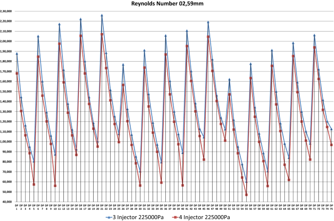

  

  Reynolds number comparison chart at plane 2.59 mm

  Fig. 21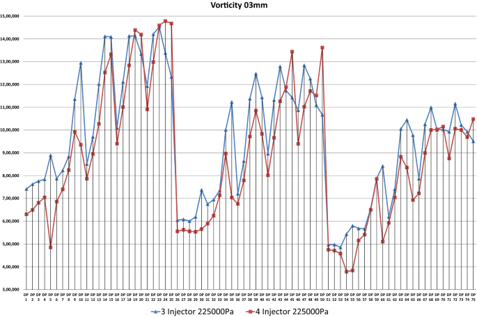

  

  Vorticity comparison chart at plane 3 mm

  Fig. 22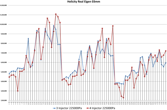

  

  Helicity comparison chart at plane 3 mm

• Some of the configuration parameters from the nozzle formed by the structural change, air intake into the nozzle from the outside on fiber inlet boundary layer. In some configurations, on the contrary, air is ejected from the nozzle to the outside environment (Fig. 8). There is only air intake from the outside to the twisting room and no air discharge to the outside environment is expected. It is thought that the outflow of air from the fiber inlet will have a negative effect on the yarn twist and hairiness. As seen from the graph in Fig. 8, in all configurations where the bending chamber diameter is Ø3 mm (DP 51–DP 75), in contrast to the air discharge from fiber inlet to the outside, it is seen that the air intake from the external environment into the twisting chamber is more dominant. It is recommended that the diameter of the nozzle twisting chamber should be at least Ø3 mm to minimize the air discharge from the fiber inlet to the outside environment according to the graph in Fig. 8. In addition, the highest swirling number (Sn) and the geometric swirling number (Sg) are seen in configurations where the twisting chamber is Ø3 mm.

• Increase of twist chamber diameter increases swirling number (Sn) and geometric swirling count (Sg) values. But, velocity dependent vorticity and helicity real eigen values are decreases.

• To understand the significant properties of yarn quality such as values of swirling number (Sn) and geometric swirling number (Sg) or values such as vorticity and helicity real eigen and to determine an optimum nozzle shape, should be supported by experimental studies that affect yarn quality.

References

Guo HF, Yu CW, Xu BG, Li SY (2011) Effect of the geometric parameters on a flexible fiber motion in a tangentially injected divergent swirling tube flow. Int J Eng Sci 49:1033–1046. https://doi.org/10.1016/j.ijengsci.2011.06.002
Weber R, Boysant F, Swithenbankt J, Roberts PA (1986) Computations of near field aerodynamics of swirling expanding flows. https://doi.org/10.1016/S0082-0784(88)80376-X
Hilsch R (1947) The use of the expansion of gases in a centrifugal field as cooling process. Rev Sci Instrum 18:108–113. https://doi.org/10.1063/1.1740893
Lucca-Negro O, O’Doherty T (2001) Vortex breakdown: a review. Prog Energy Combust Sci 27:431–481. https://doi.org/10.1016/S0360-1285(00)00022-8
Yilmaz D, Usal MR (2011) A comparison of compact-jet, compact, and conventional ring-spun yarns. Text Res J 81:459–470. https://doi.org/10.1177/0040517510385174
Wang X, Miao M, How Y (1997) Studies of JetRing spinning part I: reducing yarn hairiness with the JetRing. Text Res J 67:253–258. https://doi.org/10.1177/004051759706700403
Sheen HJ, Chen WJ, Jeng SY, Huang TL (1996) Correlation of swirl number for a radial-type swirl generator. Exp Therm Fluid Sci 12:444–451. https://doi.org/10.1016/0894-1777(95)00135-2
Guo HF, Chen ZY, Yu CW (2009) Simulation of the effect of geometric parameters on tangentially injected swirling pipe airflow. Comput Fluids 38:1917–1924. https://doi.org/10.1016/j.compfluid.2009.05.001
Chang F, Dhir VK (1994) Turbulent flow field in tangentially injected swirl flows in tubes. Int J Heat Fluid Flow 15:346–356. https://doi.org/10.1016/0142-727X(94)90048-5
Guo HF, Xu BG, Yu CW, Li SY (2011) Simulating the motion of a flexible fiber in 3D tangentially injected swirling airflow in a straight pipe—Effects of some parameters. Int J Heat Mass Transf 54:4570–4579. https://doi.org/10.1016/j.ijheatmasstransfer.2011.06.021
Chen J, Haynes B, Fletcher D (2006) A numerical and experimental study of tangentially injected swirling flow. In: 2nd International conference on CFD minerals and process industries, pp 485–490
Parra-Santos MT, Perez R, Mendoza V et al (2016) Influence of swirl number on semi-confined flames. Int J Appl Math Electron Comput 4:65–67. https://doi.org/10.18100/ijamec.69979
Release 16.2 - © SAS IP I Turbulence Modeling in Swirling Flows. https://www.sharcnet.ca/Software/Ansys/16.2.3/en-us/help/flu_ug/flu_ug_uns_sec_rot_swirl_turb.html. Accessed 3 Oct 2018
Gulsevincler E (2013) Turbulence models and simulations in compressible fluid flow, M.Sc. Thesis. Suleyman Demirel University
Cebeci T (2003) Turbulence models and their application: efficient numerical methods with computer programs. Springer, New York
Wilcox DC (1988) Reassessment of the scale-determining equation for advanced turbulence models. AIAA J 26:1299–1310
Menter F (1993) Zonal two equation kw turbulence models for aerodynamic flows. In: 23rd Fluid dynamics, plasmadynamics, and lasers conference, p 2906
Ansys Inc (2001) Ansys fluent theory guide. In: Ansys fluent theory guide, pp 39–43
Pandey KM, Roga S, Choubey G (2015) Computational analysis of hypersonic combustor using strut injector at flight Mach 7. Combust Sci Technol 187:1392–1407. https://doi.org/10.1080/00102202.2015.1035371
Akansu SO (2006) Heat transfers and pressure drops for porous-ring turbulators in a circular pipe. Appl Energy 83:280–298. https://doi.org/10.1016/j.apenergy.2005.02.003
Eberlinc M, Širok B, Hočevar M, Dular M (2009) Numerical and experimental investigation of axial fan with trailing edge self-induced blowing. Eng Res 73:129–138. https://doi.org/10.1007/s10010-008-0086-8
Mani S, Sanal Kumar VR (2015) 3D flow visualization and geometry optimization of cavity based scramjet combustors using k-? Model. In: 51st AIAA/SAE/ASEE joint propulsion conference. American Institute of Aeronautics and Astronautics
Ajith S, Mani S, Tharikaa R, et al (2015) Diagnostic investigation of flame spread mechanism in dual-thrust solid propellant rocket motors. In: 51st AIAA/SAE/ASEE joint propulsion conference. American Institute of Aeronautics and Astronautics
Mahmood S, De-Bo H (2011) Resistance calculations of trimaran hull form using computational fluid dynamics. In: Proceedings of the 4th international joint conference on computer sciences and optimization, CSO 2011, pp 81–85. https://doi.org/10.1109/CSO.2011.225
Simic M, Herakovic N (2015) Reduction of the flow forces in a small hydraulic seat valve as alternative approach to improve the valve characteristics. Energy Convers Manag 89:708–718. https://doi.org/10.1016/j.enconman.2014.10.037
Deng R, Jin Y, Kim HD (2017) Numerical simulation of the unstart process of dual-mode scramjet. Int J Heat Mass Transf 105:394–400. https://doi.org/10.1016/j.ijheatmasstransfer.2016.10.004
Gupta A, Kumar R (2007) Three-dimensional turbulent swirling flow in a cylinder: experiments and computations. Int J Heat Fluid Flow 28:249–261. https://doi.org/10.1016/j.ijheatfluidflow.2006.04.005
Soltanipour H, Mirzaei I, Choupani P (2010) The effect of triangular vortex generators on turbulent flow and heat transfer in a channel, pp 505–510
Lee Y-T, Lim H-C (2013) Effect of turbulent boundary layer on the surface pressure around trench cavities. J Mech Sci Technol 27:2673–2681. https://doi.org/10.1007/s12206-013-0711-9
Gotzfried K (1984) Patent: US4444003A Turbulent spinning apparatus for the production of yarn
Pacholski J, Kujawski Z, Janczyk R, Bartczak M (1981) Patent: US4253297A, Method and apparatus for the production of core yarn
Jozwicki R, Kluska B, Radom C, Pacholski J (1982) U.S. Patent No. 4,319,448. U.S. Patent and Trademark Office, Washington, DC
Rohlena V (1975) Open-end spinning. Elsevier, Amsterdam
Yilmaz D, Usal MR (2012) Effect of nozzle structural parameters on hairiness of compact-jet yarns. J Eng Fiber Fabr 7:56–65
Yilmaz D, Usal MR (2013) Investigation of yarn properties of modified yarn spinning systems with air nozzle attachment. Fibres Text East Eur 98:43–50
Yilmaz D (2011) Development and numerical modelling of plied yarn production process based on the usage of high velocity air, Ph.D. Thesis. Suleyman Demirel University
Yilmaz D, Usal MR (2012) A study on siro-jet spinning system. Fibers Polym 13:1359–1367. https://doi.org/10.1007/s12221-012-1359-2
Acknowledgements
This work is supported by grants from the Unit of Scientific Research Projects of Isparta (Suleyman Demirel University) in Turkey [Project 4995-D1-17].
Funding
This research was funded by the Unit of Scientific Research Projects of Isparta (Suleyman Demirel University) Foundation for researcher [Grant Number BAP 4995-D1-17].
Author information
Authors and Affiliations
Contributions
EG designed the model of the parametric nozzle shape; DY determined the parametric study value range; EG and MRU performed the parametric CFD analysis; EG, MRU and DY analyzed the data; EG wrote the paper. MRU and DY checked and revised the paper.
Corresponding author
Ethics declarations
Conflict of interest
The authors declared that they have no conflict of interest.
Additional information
Publisher's Note
Springer Nature remains neutral with regard to jurisdictional claims in published maps and institutional affiliations.
Rights and permissions
About this article
Cite this article
Gulsevincler, E., Usal, M.R. & Yilmaz, D. The effects of structural parameters on tangentially injected highly swirling turbulent tube air flow. SN Appl. Sci. 1, 835 (2019). https://doi.org/10.1007/s42452-019-0850-4
Received:
Accepted:
Published:
DOI: https://doi.org/10.1007/s42452-019-0850-4