Morphometric analysis for prioritizing sub-watersheds and management planning and practices in Gidabo Basin, Southern Rift Valley of Ethiopia

Abstract

Characterization and prioritization of watersheds has gained importance for proper planning and management of natural resources in sustainable development. Implementation of management practices over a larger area at the same time is inaccessible and uneconomical. So, it has required applying a viable technique for prioritization of critical sub-watersheds. Thus, the present study was aimed to prioritizing erosion-prone sub-watersheds using morphometric analysis. Advanced space-borne thermal emission and reflection radiometer of 30m resolution DEM has used to generate drainage networks and delineation of sub-watersheds using ArcGIS software. The important derived morphometric parameters have computed on the base of already developed mathematical formulae and methods. The study area (a watershed) has classified into seven interesting sub-watersheds, which have ordered SW1–SW7. The very important quantitative watershed aspects such as linear, relief and areal have been taken in consideration, and eighteen morphometric parameters have been selected and used for ranking and prioritizing of sub-watersheds. In this regard, sub-watersheds (SW7, SW3 and SW4) and (SW5, SW6 and SW2) have categorized into higher and medium priorities, whereas sub-watershed (SW1) has assigned at lower priority. This implied that SW1 is relatively sustainable than others, on the contrary, SW7 is relatively affected sub-watershed by runoff and soil erosion that needs first priority for management practices. Therefore, the study proposes a useful soil and water conservation practices such as bunds, check dams, micro-basins and multipurpose tree species planting based on suitable location and design parameters. The decision makers should optimally allocate the investments according to this final priority. And it has required to monitor and evaluate due to environmental sound, economical viable and socially acceptable. Also it has required developing an integrated approach for characterizing and prioritizing of sub-watersheds.

Introduction

A watershed is defined as any surface area from which runoff resulting from rainfall is collected and drained through a common confluence point (Desta et al. 2005). It is similar to a drainage basin or a catchment area. The study of watershed plays an important role for any kind of developmental activities and sustainable management (Sangma and Guru 2020). Because, watershed is made up of natural resources, such as water, soil and vegetation resources. People interact with land resources in a watershed; due to their socioeconomic activities, watershed is the hydrological, bio-physical and socioeconomic units. This implies that, a watershed consists of both natural and social systems; it forms unique and interacted landscape hierarchies. Hence, we can use a watershed as an ideal unit for planning and management of natural resources. Also it has been used as a comprehensive development concept and a strategy to achieving food security (German et al. 2007; Mekonnen and Fekadu 2015; Worku and Tripathi 2015). For example, a watershed harmonizes the use of soil, water and vegetation if we conserve these resources; it optimizes productivity with minimum environment impacts (Sharma et al. 2005; Kerr 2007; Alemu and Kidane 2014). Therefore, watershed management is aimed to protect the environment and enhancing food security (Kumar and Palanisami 2009).

The history of watershed management was date back to 5000 years old; since agricultural production and the origin of modern approach has started in the last quarter of nineteenth century (Darghouth et al. 2008), it became prominent in developing countries in the 1970s and 1980s. By following the 1984/1985 drought and famine happened to Ethiopia, watershed development concept has started since 1980s (Desta et al. 2005). Since and then, although watershed management practices showed positive results to rehabilitate severely degraded land, enhancing agricultural productivity and diversifying farmers income, it has no more achievements as expected due to different factors like top-down approach and lack of local community participation (Chimdesa 2016). Moreover, it has required supporting through research and educational institutions.

All watershed management activities cannot be carried out at the same time over a larger area. Because it is a very complex and has variable characteristics, it is not accessible and uneconomical to apply all at once. Firstly, it is essential to understand existing watershed characteristics, logics and potentials. Then, it is a prerequisite to select and apply viable parameters for characterizing and prioritizing sensitive sub-watersheds. Here, watershed characterization is defined as the process involves gathering information and describing the very nature of a watershed and its components. This offers the bio-physical and socioeconomic components of the watershed to determining vulnerability issues and opportunities for developing interventions. Watershed prioritization is the ranking of different sub-watersheds of a watershed according to their order in which they have to take for soil and water conservation (Iqbal and Sajjad 2014). Also, this required to prepare comprehensive watershed management planning.

At the present, analyzing watershed morphometry is used as a basic and the most logical choice (Imran et al. 2011); it is the most viability method and relatively simple approach to describe quantitative watershed characteristics (Mesa 2006; Deepak 2015; Umer et al. 2015). Since watershed morphometric analysis only depends on drainage system and spatial relationship among streams, it has also characterized by using other data like soil and land use maps (Kiran and Srivastava 2012). The morphometric analysis is very much useful in dealing with where information accessibility is limited data and other resources, and high soil variety (Meshram et al. 2020; Sangma and Guru 2020; Rahmati et al. 2019). Sub-watersheds can be categorized using morphometric parameters without facing with high cost and a waste of time (Meshram et al. 2019). Moreover, morphometric analysis is a comparative evaluation and understanding of landforms, soil properties, hydrological and erosion characteristics of sub-watersheds, which have to assess and compare through morphometric parameters (Dar et al. 2013; Amulya et al. 2018). Morphometric feature of a watershed typically covers the quantitative aspects and physical characteristics of the watershed. It is static criteria or natural characteristics that do not change easily over time. It also required to prioritize sub-watersheds for effective natural resources management (Javed et al. 2009; Sharma et al. 2010; Ajay et al. 2014; Ayele et al. 2017).

Morphometric analysis is the measurement and mathematical analysis of earth’s surface, shape and dimension of landforms (Clarke 1996; Agarwal 1998; Obi et al. 2002). It computes quantitative attributes of landscapes such as: linear, areal and relief aspects of a watershed. Watershed morphometric parameters are either direct or inverse relationship of runoff, peak to discharge, lag time, soil erosion and sedimentation risks (Nookaratnam et al. 2005; Gajbhiye and Sharma 2017), and these can be used to identify and prioritize critical sub-watersheds. Watershed prioritization is one of the most important processes in natural resource management system especially in areas of sustainable watershed development and planning (Balasubramanian et al. 2017). For instance, Welde (2016) has attempted to identifying and prioritizing sub-watersheds based on their annual sediment yield; Abdulkareem et al. 2018 and Singh and Singh 2014 have attempted to prioritizing sub-watersheds based on peak discharge and lag time. Morphometric parameters are highly efficient in identifying erosion-prone areas (Meshram et al. 2020). Morphometric analysis is significant to identify and assess seasonal changes in drainage basin characteristics, understand the groundwater potentialities and address issues related to floods proneness during the high flows (Mangan et al. 2019; Choudhari et al. 2018). Moreover, various studies have used to prioritizing and comparing sub-watersheds through analyzing their morphometry (Sharma et al. 2010; Kumar et al. 2015; Thapliyal et al. 2017; Kumar and Lal 2017). In general, watershed morphometric study is crucial in providing significant information about the drainage network, hydro-geo-morphometric characteristics and natural hazards of the basin for sustainable natural resources management planning processes (Karabulut and Özdemir 2019; Gunjan et al. 2019; Nitheshnirmal et al. 2019). And some have used both morphometric and land use characteristics (Javed et al. 2009; Ajay et al. 2014; Iqbal and Sajjad 2014; Suji et al. 2015).

Unfortunately, there were few studies conducted in our country, Ethiopia. Therefore, this study aimed to analyze watershed morphometric characteristics for prioritizing sub-watersheds for management planning in Gidabo sub-basin, rift valley of Ethiopia. The study has attempted to answer the research questions like, why and how we analyze watershed morphometric characteristics. For the advancement, Geographical Information System (GIS) and Remote Sensing (RS) technique has been used for this study. Combining with the past studies, this research provides essential information on the scholars, decision makers, local communities and the others. It contributes to watershed science with regard to integrated designing and implementing programs, and for the scaling up of good management practices. It also benefits the researchers that deal with similar research topics for other areas.

Methodology

Study area

The study watershed is found in Gidabo Sub-Basin, Rift Valley of Ethiopia. It locates at 359 km from Addis Ababa, the capital city of Ethiopia. It covers 782.574 km². It bounds with two regional states (SNNP and Oromia), three administrative zones (Gedeo, Sidama and West Guji), eight districts (Bule, Wenago, Dilla zuria, Dera, Aleta wondo, Chuko, Hula and Abaya) and it includes 98 kebeles. An estimated total population is 659,734 (Male: 328, 852 and Female: 330,882) (CSA 2013). It locates between 6° 10′ 30″ to 6° 36′ 00″ N and 38° 10′ 00″ to 38° 32′ 00″ E (Fig. 1). Altitude ranges from 1197 m.a.s.l (at Semero Gamibela kebele) to 3025 m.a.s.l (at Kochore kebele), and the slope is range from 0° to 62°. According to Bekele-Tesemma (2007) traditional agro-climatic classification, the watershed covers the three agro-climatic zones, namely moist lowland (Kolla), moist mid-highland (Weyna dega) and moist highland (Dega). The area has categorized into three agroforestry systems, such as: Enset-based (> 2300–3200 m.a.s.l), Coffee-enset-based (1500–2300 m.a.s.l) and Fruit-coffee based altitude of less than 1500 m.a.s.l (Kanshie 2002; Kura 2013; Negash 2013). The mean annual rainfall and temperature is 1200–1800 mm and 15–27 °C, respectively (Erifo and Amanuel 2015; Keffale et al. 2017). The area is among the bimodal regions of Ethiopia. July to December is the main rainy season, while March to May is the small rainy season of the area. The watershed drains with perennial rivers like: Sala, Darra and Majege rivers. The area covers a variety of volcanic rocks and to a minor part by lacustrine sediments (Mechal et al. 2015). According to FAO (1988) soil classification, the major soil units of the area are Haplic Luvisols, Chromic Luvisols and Rhodic Nitosols. The area is known by mixed farming and evergreen agroforestry systems. Coffee (Coffea arabica) and enset (Ensete ventricosum) are the dominant perennial crops of the area. Barely, maize, wheat, teff, peas, haricot beans, groundnut, tomato, onion, potato, pepper, cabbage, etc. are the crops grown in the area; and cattle, sheep, goats, equines and chickens are the livestock raring in the area. Millettia ferruginea, Syzygium guineense, Albizia gummifera, Cordia africana, Aningeria attissima, Polyscias ferruginea, Croton macrostachys, Erythrina abbyssnica, Podocarpus flactus, Eucalyptus spp. and bamboo are the tree species as well as banana, mango, avocado, guava and papaya are the fruit trees grown in the area.

Fig. 1

(Source: Authors)

Location map of the study area.

Watershed morphometric parameters

Advanced space-borne thermal emission and reflection radiometer of 30 m resolution (ASTER_DEM) was used to generate drainage networks and delineate interested sub-watersheds using ArcGIS10.3 software. Toposheets with 1:50,000 scale of the study area have obtained from Ethiopian National Map Authority. Field visits and control points have used to verify the ground truth by using Geographical Positioning System (GPS) tool. The very important quantitative morphometric parameters are selected and used for this analysis. These would be categorized into linear, relief and areal aspects. Because they have direct or inverse relationship with runoff, peak discharge and soil erosion risks (Nookaratnam et al. 2005; Javed et al. 2009; Singh and Singh 2014; Gajbhiye and Sharma 2017), then these have used to prioritize more sensitive sub-watersheds. Based on computed basic parameters due to ASTER_DEM and GIS software, the derived parameters have been calculated based on the mathematical formulae and methods which have already been developed and summarized in Table 1. Other methods, approaches and information have also reviewed from related literature. See Fig. 2: the methodological flowchart used for watershed morphometric analysis.

Table 1 Formulae and methods adopted to compute watershed morphometric parameters

Fig. 2

Methodological flowchart for watershed morphometric analysis

Results and discussion

The study watershed was delineated to seven sub-watersheds with coded as SW1 to SW7. Predominantly it is dendritic to sub-dendritic drainage pattern which intersecting branches at acute angles. This indicates the presence of homogenous rocks and uniform soil type in mountainous and hilly area. Map of each sub-watersheds and drainage networks is located in Fig. 3.

Fig. 3

Map of sub-watersheds and drainage networks

Watershed morphometric analysis

Depending on the formulae and methods described in Table 1, the computed results of morphometric parameters are summarized in Table 2, and their implications are also discussed.

Table 2 Computed results of watershed morphometric parameters

Basic parameters

Watershed area (A) is the total area projected upon horizontal plane of a watershed. It is the most important watershed characteristics since it directly reflects volume of water in a watershed. Larger size intercepts greater volume of rainfall, higher runoff and peak discharge. Sometimes, the smaller size has also recorded maximum flooding and sedimentation. This is due to other watershed morphometric characteristics like stream networks, shape and length and relief parameters. In present study, the area ranges 81.90–151.16 km², the smallest at SW6 and the largest at SW7.

Watershed perimeter (P) is length of delineated watershed boundary. It also represents watershed size. The perimeter ranges 46.34–97.21 km; the shortest at SW6 and the longest at SW7.

Watershed length (L_b) it is the longest dimension of basin parallel to the principal drainage channel (Schumm 1956). It shows the main channel of watershed in which the greatest volume of water travels. In this regard, the length of sub-watersheds is the longest at SW7 (22.69 km) and the shortest at SW6 (16.02 km).

Watershed relief (B_h) is the elevation between outlet and the highest point on the perimeter of a watershed. Here, at the study area, elevation ranges 1200–3020 m.a.s.l.

Stream order (U) is a measure of the position of a stream in the hierarchy of tributaries. Stream ordering or stream categorization is based on the number and the type of tributary junctions, which is the initial step in morphometric analysis. The streams are given order designation based on Strahler (1964) method. The smallest finger type and not branched tributaries are nominated as first stream orders; where two first stream orders join, these are second stream orders; where the second stream orders join, these are third stream orders, and so on. It increases from upstream to downstream due to geomorphology of a watershed, and the highest order of stream segment is the main channel in which all discharges, runoff and sediment pass (Kumar and Lal 2017). The main and highest order (5th order) is shown at SW1 and SW7; and others with the 4th order.

Stream number (N_u) is the number of stream segments present in each order. The relationship between the number of streams of a given order and the stream order form an inverse geometric series (Horton 1945). It informs about surface runoff features. For example, a watershed with maximum numbers of first-order streams indicates highest permeability and infiltration rate, and erodible topography. A watershed with higher in number and order of streams is characterized by soft shale and slate rocks (Biswas 2016). In the present study, number of first stream order is highest and lowest at SW7 (68) and SW6 (33), respectively.

Stream length (L_u) is the average lengths of streams of each of the different orders in a drainage basin that tends closely to approximate a direct geometric series in which the first term is the average length of streams of the 1st order. Stream length is the highest in first-order consequently it increases as stream order increases (Horton 1945). Relatively, shorter the stream length is at area of steep slopes and finer texture, whereas longer the stream lengths are at area of lower slopes (Strahler 1964). Besides, it measures hydrological characteristics and bedrock formation of the area. Relatively, the permeable bedrock and well-drained watershed is formed a smaller in stream number and longer in stream length and the vice versa (Sethupathi et al. 2011). For the current study, the longest and the shortest stream lengths of all orders are at SW7 (158.75 km) and SW6 (85.761 km), respectively (see Table 3).

Table 3 Stream orders and numbers

Derived parameters

Linear aspects

Bifurcation ratio (Rb) is the ratio between total numbers of streams in a given order (N_u) to the number of next higher order (N_u + 1) (Schumm 1956). R_b is related to the branching pattern of a drainage network which shows degree of integration between streams of various orders (Horton 1945). Lower R_b values show structurally less disturbed watersheds without any distortion in drainage pattern (Suji et al. 2015). In the present study, R_b value is the highest and lowest at SW1 (14.33) and SW6 (10.21), respectively. This implied that SW1, SW7 and SW3 are relatively more disturbed sub-watersheds than others, whereas SW6, SW4 and SW5 are relatively sustainable sub-watersheds.

Stream length ratio (R_l): is the ratio of mean stream length of a given order (L_u) to the mean stream length of the next smaller order (L_u − 1) (Horton 1945). In fact, the mean length of a stream of any given order is always greater than the mean length of a stream of the next lower order. It gives an idea about chronological developments of the stream segments and relative permeability of the rock formation in a watershed.

According to Horton (1945), two fundamental laws are related to the stream numbers and lengths of different orders in a drainage basin.

• 1. Law of stream numbers: the relation between streams number of a given order, and stream order in terms of an inverse geometric series, in which bifurcation ratio is the base. This law was checked for all sub-watersheds and the results are in line with that of Horton’s law of stream numbers (Fig. 4), where the number of streams and stream order exhibited well inverse and strong relationship with coefficient of determination (R²) ranges from 0.78 (at SW1) to 0.99 (at SW3).

  Fig. 4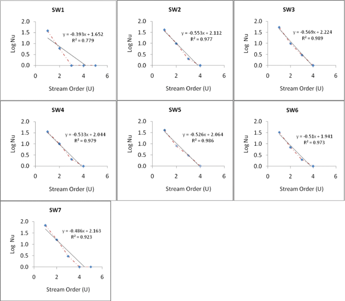

  

  Relationship between stream order and stream number

• 2. Law of stream lengths: the average length of streams of a given order in terms of stream order, average length of streams of 1st order, and the stream length ratio, this law takes the form of a direct geometric series. This law was also checked for all sub-watersheds and the result deviated from that of Horton’s law of stream length (Fig. 5), where the stream length and stream order show weak relationship with coefficient of determination (R²) ranges from 0.36 (at SW1) to 0.83 (at SW6). Here, the deviation and the differences among sub-watersheds may indicate the sub-watersheds are varying in lithology (bedrocks) and presence of geological control in addition to other environmental factors, for example water erosion processes.

  Fig. 5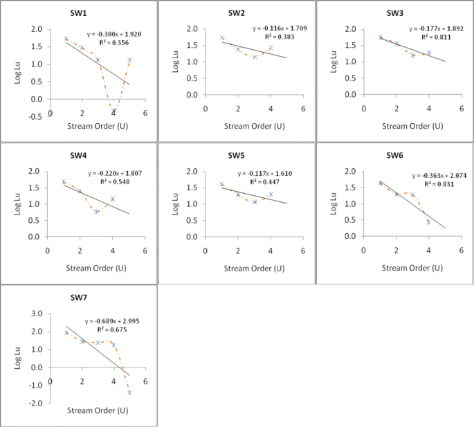

  

  The relationship between stream order and stream length

Stream frequency (F_s): is total number of streams per unit area (Horton 1945). Values of drainage density and stream frequency for small and large drainage basins are not directly comparable because they usually vary with the size of the drainage area. But stream frequency exhibits positive correlation with drainage density to indicate the increase stream population drainage density at the same (Suji et al. 2015). In this analysis, stream frequency is higher at SW7, SW5 and SW6; and lower at SW1, SW2 & SW3.

Drainage density (D_d) is the total length of streams per unit area (Horton 1945). It represents channels development and their spacing closeness in watershed. Here, drainage density is higher at SW7, SW6 and SW2; and lower at SW5, SW3 and SW1.

Drainage texture (D_t) is the total number of streams per perimeter of a watershed (Horton 1945). It shows the relative spacing of drainage lines. In the present study SW7, SW6 & SW4 are higher; and SW1, SW2 and SW3 are lower in drainage texture.

Length of overland flow (L_o) is roughly equal to half of the reciprocal of drainage density (Horton 1945). It is used to describe the length of flow of water over the ground before it becomes concentrated in definite stream channels. In the study area, SW5, SW3 and SW1 are higher and SW7, SW6 and SW2 are lower in length of overland flow, respectively.

Drainage intensity (D_i) is the ratio of stream frequency to the drainage density (Faniran 1968). A watershed with low values in drainage density, drainage texture and drainage intensity is sensitive to flooding, erosion and landslide. In the present analysis, SW5, SW7 and SW3 are higher, whereas SW1, SW2 and SW4 are lower in drainage intensity.

Rho coefficient (ρ): is the ratio between the stream length ratio and the bifurcation ratio. It is an important parameter to relate drainage density to physiographic development which determines the storage capacity of drainage network and ultimate degree of drainage development (Horton 1945). Here, Rho coefficient is higher at SW1, SW2 and SW5, while lower at SW6, SW7 and SW3. This suggests SW1 has the highest storage capacity during floods and attenuation effects of erosion during elevated discharge.

Infiltration number (I_f) is the product of drainage density and stream frequency. At higher infiltration number, lower the infiltration rate and higher in surface runoff (Faniran 1968). In the present study, SW7, SW6 and SW5 are higher, and SW1, SW2 and SW3 are lower values in infiltration number. This indicates that SW7, SW6 and SW5 are relatively dominating higher values in linear aspects while SW1, SW2 and SW3 are lower characteristics.

Areal aspects

Circulatory ratio (R_c) is ratio of watershed area to area of a circle having the same circumference as perimeter of the watershed (Miller 1953). A circular watershed is the most susceptible to peak discharge because it will yield the shortest time of concentration. Lower, medium and higher values of R_c indicate young, mature and old stages of watershed development. SW1, SW2 and SW3 are lower, while SW6, SW4 and SW7 show higher values in circulatory ratio at the study area.

Elongation ratio (R_e) is the ratio between the diameter of a circle of the same area as the watershed and the maximum length of the watershed (Schumm 1956). It usually ranges from 0.6 to 1.0. If the value is equal to one, a watershed is equal from all sides. Re is lower values at SW7, SW3 and SW1, whereas SW6, SW4 and SW5 have higher values of elongation ratio at the study area.

Form factor (F_f) is the ratio of watershed area (A) to the square of watershed length (L_b). Smaller the value of form factor, more the elongated watershed (Strahler 1964). A watershed with higher form factor has high peak discharge in a short period of time (Horton 1945). Here, value of Ff is lower at SW7, SW3 and SW2 while SW6, SW4 and SW5 are higher in form factor in the study area.

Lemniscate’s ratio (K) is used to determine gradient of the watershed (Chorley et al. 1957). In the present study, SW6, SW4 and SW5 have lower K values, whereas SW7, SW3 and SW2 have the higher values.

Compactness coefficient (C_c) is the ratio of perimeter of watershed to circumference of equivalent circular area of the watershed (Horton 1945). It is an independent of watershed size, but it depends on the slope. In the present study, value of Cc is lower at SW6, SW4 and SW7 whereas SW1, SW2 and SW3 are relatively higher in compactness coefficient. In general, regarding to areal and shape aspects of the sub-watersheds, SW7, SW6 and SW3 have dominated with lower values whereas SW4, SW2 and SW3 have relatively higher values.

Relief aspects

Relief ratio (R_h) is the ratio of maximum watershed relief to the maximum watershed length, which is parallel to the principle drainage line. It measures overall steepness of a watershed, and it is an indicator of erosion process and intensity on watershed slopes (Schumm 1956). R_h value is higher value at SW6, SW4 and SW2, whereas SW1, SW5 and SW7 have lower value of relief ratio at study area.

Relative relief (R_hp) has calculated by using perimeter and watershed relief (Melton 1957). In the present study, SW6, SW4 and SW7 have higher while SW1, SW2 and SW3 have lower values in relative relief.

Ruggedness number (R_n) is the product of maximum basin relief and drainage density (Strahler 1964). It combines slope steepness and length. Its higher values occur when slopes are not only steep but long as well. It has higher values at SW7, SW3 and SW6, and it has lower values at SW1, SW5 and SW4 in the study area. In general, regarding relief aspects of sub-watersheds, SW6 and SW4 are dominating the higher values whereas SW1 and SW5 are relatively lower values.

Ranking and prioritization of sub-watersheds

Linear and relief parameters have direct relationship with soil erodibility (Nookaratnam et al. 2005; Singh and Singh 2014; Sujatha et al. 2015), the highest their value shows the most erodible soil in a watershed. Therefore, a sub-watershed showed the highest value in linear and relief parameters has rated at first rank, second higher value has rated as second rank and so on; and the least value has rated at last the rank. In the contrary, areal/shape parameters have inverse relationship with soil erodibility (Javed et al. 2009; Raja et al. 2017); the lowest their value the most erodible soil in a watershed. Thus, a sub-watershed showed the lowest value in areal/shape parameters has rated at first rank, the next lower value has rated at second rank and so on, then the highest value has rated at the last rank. Compound method of averaging value was used in this study, because it has expected all morphometric parameters have equal importance for final ranking (Ajay et al. 2014; Farhan 2017). After ranking of all (seven) sub-watersheds based on every single parameter, the ranking values for all parameters of each sub-watershed have added and divided by the number of all parameters, in this case it has divided by eighteen; and then to arrive at compound value. So that, the sub-watershed with the least compound value has assigned at the highest priority and denoted by number 1, the next higher value has denoted by number 2 and so on, then the sub-watershed that got the highest compound value has assigned at the last priority number (Ayele et al. 2017; Sheikh et al. 2017; Thapliyal et al. 2017; Kumar and Lal 2017). This implies that, the highest priority indicates the greatest degree of runoff, peak discharge and soil erosion risks in that sub-watershed. Thus, it is important to plan proper land and water management practices for each sub-watersheds as per their sensitivity ranks. Eighteen morphometric parameters were selected and used for ranking and prioritizing of sub-watersheds based on their values obtained from the calculation (see Table 4).

Table 4 Computed parameters used for ranking and prioritization of sub-watersheds

Figure 6 shows the final priority map of sub-watersheds. SW7, SW3 and SW4 are relatively the most susceptible to land degradation being prone to soil erosion, respectively. This is due to their inherent geomorphometric characteristics. Hence, they need immediate attention for soil and water conservation measures or practices according to the final priority.

Fig. 6

Map of prioritized sub-watersheds through morphometric parameters

Conclusion and recommendations

Morphometric analysis is very important approach to describe physical and quantitative characteristics of a watershed. Also it has been used to prioritize sub-watersheds for effective natural resources management. Rather than conventional methods, Remote Sensing and Geographical Information System application enable to estimate watershed morphometric aspects. After prioritization of critical sub-watersheds, it is crucial to prepare a comprehensive watershed management planning and implementation. Analyzing watershed morphometry is not enough for characterizing and prioritizing of sub-watersheds, but it has required other an integrated approach, which includes land use and land cover changes, estimation of runoff and sediment yield. Here, the study proposes a useful tool to define areas for planning the strategies to control soil erosion and promote soil conservation. This may include both physical and biological measures such as constructing bunds, check dams, micro-basins and planting multipurpose tree species based on suitable location and design parameters. Decision makers should optimally allocate the investments to critical sub-watersheds in an economically effective and technically efficient manner. Finally, it has required to monitor and evaluate as per environmental sound, economical viable and socially acceptable.

References

Abdulkareem JH, Pradhan B, Sulaiman WNA, Jamil NR (2018) Quantification of runoff as influenced by morphometric characteristics in a rural complex catchment. Earth Syst Environ 2(1):145–162. https://doi.org/10.1007/s41748-018-0043-0
Agarwal CS (1998) Study of drainage pattern through aerial data in Naugarh area of Varanasi district, UP. J Indian Soc Remote Sens 26:169–175
Ajay P, Mahmood K, Vijay S, Paru PTh, Joy J, Nayan P, Kalubarme MH (2014) Morphometric and land use analysis for watershed prioritization in Gujarat State, India. Int J Sci Engine Res 5(2):1–7
Alemu B, Kidane D (2014) The implication of integrated watershed management for rehabilitation of degraded lands: case study of ethiopian highlands. J Agric Biodivers Res 3(6):78–90
Amulya GV et al (2018) GIS-based morphometric analysis of sub-watershed of Gurupura River, Dakshina Kannada District. Int J Recent Sci Res 9(6):27545–27549
Ayele AF, Hiroshi Y, Katsuyuki Sh, Nigussie H, Kifle W (2017) Quantitative analysis and implications of drainage morphometry of the Agula watershed in the semi-arid northern Ethiopia. Appl Water Sci 7:3825–3840
Balasubramanian A, Duraisamy K, Thirumalaisamy S, Krishnaraj S, Yatheendradasan RK (2017) Prioritization of subwatersheds based on quantitative morphometric analysis in lower Bhavani basin, Tamil Nadu, India using DEM and GIS techniques. Arab J Geosci. https://doi.org/10.1007/s12517-017-3312-6
Bekele-Tesemma A (2007) Useful trees of Ethiopia: identification, propagation and management in 17 agroecological zones. RELMA in ICRAF Project, Nairobi
Biswas SS (2016) Analysis of GIS based morphometric parameters and hydrological changes in Parbati River Basin, Himachal Pradesh, India. J Geogr Nat Disasters 6:175. https://doi.org/10.4172/2167-0587.1000175
Chimdesa G (2016) Historical perspectives and present scenarios of watershed management in Ethiopia. Int J Nat Resour Ecol Manag 1(3):115–127
Chorley RJ, Malm DEG, Pogorzelski HA (1957) A new standard for estimating drainage basin shape. Am J Sci 225:138–141
Choudhari PP, Nigam GK, Singh SK, Thakur S (2018) Morphometric based prioritization of watershed for groundwater potential of Mula river basin, Maharashtra, India. Geol Ecol Landsc. https://doi.org/10.1080/24749508.2018.1452482
Clarke JI (1996) Morphometry from maps. Essays in geomorphology. Elsevier, New York, pp 235–274
CSA (2013) Federal demographic republic of Ethiopia Central Statistical Agency, Population Projection of Ethiopia for All Regions, At Wereda Level from 2014–2017. August 2013. Addis Ababa
Dar RA, Chandra R, Romshoo SA (2013) Morphotectonic and lithostratigraphic analysis of intermontane Karewa basin of Kashmir Himalayas, India. J Mt Sci 10(1):731–741
Darghouth S, Ward C, Gambarelli G, Styger E, Roux J (2008) Watershed management approaches, policies, and operations: lessons for scaling up. Water Sector Board discussion paper series, no. 11. World Bank, Washington, DC. World Bank. https://openknowledge.worldbank.org/handle/10986/17240 License: CC BY 3.0 IGO
Deepak KM (2015) The basic concept to study morphometric analysis of river drainage basin: a review. Int J Sci Res 4(7):2277–2280
Desta L, Carucci V, Wendem-Ageňehu A, Abebe Y (eds) (2005) Community based participatory watershed development: a guideline. Ministry of Agriculture and Rural Development, Addis Ababa
Erifo S, Amanuel TW (2015) Value chain analysis of bamboo production: the case of Bule Woreda, Gedeo Zone, SNNPRS. Ind Engine Lett 5(11):34–44
Faniran A (1968) The index of drainage intensity: a provisional new drainage factor. Aust J Sci 31(9):326–330
FAO (1988) Food and agricultural organization. Soil map of the world, revised legend with corrections and updates world soil resource. Report 60, FAO, Rome, Italy
Farhan Y (2017) morphometric assessment of Wadi Wala Watershed, Southern Jordan using ASTER (DEM) and GIS. J GIS 9:158–190
Gajbhiye SM, Sharma SK (2017) Prioritization of watershed through morphometric parameters: a PCA-based approach. Appl Water Sci 7(2017):1505–1519
German L, Mansoor H, Alemu G, Mazengia W, Amede T, Stroud A (2007) Participatory integrated watershed management: evolution of concepts and methods in an Eco regional program of the eastern African highlands. Agric Syst 94(2007):189–204
Gunjan P, Mishra SK, Lohani AK, Chandniha SK (2019) The study of morphological characteristics for best management practices over the Rampur watershed of Mahanadi River Basin using prioritization. J Indian Soc Remote Sens. https://doi.org/10.1007/s12524-019-01061-y
Horton RE (1945) Erosional development of streams and their drainage basins; hydrophysical approach to quantitative morphology. Geol Soc Am Bull 56(3):275–370
Imran MM, Sultan MB, Kuchay AN (2011) Watershed based drainage morphometric analysis of Lidder catchment in Kashmir valley using geographical information system. Recent Res Sci Technol 3(4):118–126
Iqbal M, Sajjad H (2014) Watershed prioritization using morphometric and land use/land cover parameters of Dudhganga Catchment Kashmir Valley India using spatial technology. J Geophys Remote Sens 3:115
Javed A, Khanday MY, Ahmed R (2009) Prioritization of sub-watersheds based on morphometric and land use analysis using remote sensing and GIS techniques. J Indian Soc Remote Sens 37:261–274
Kanshie KT (2002) Five thousand years of sustainability? A case study on Gedeo land use (Southern Ethiopia). Treebook 5. Treemail Publishers, Heelsum
Karabulut MS, Özdemir H (2019) Comparison of basin morphometry analyses derived from different DEMs on two drainage basins in Turkey. Environ Earth Sci. https://doi.org/10.1007/s12665-019-8585-5
Keffale MB, Shabula Z, Tamerat NB (2017) Prevalence of bovine trypanosomiasis in Dara District Sidama Zone, Southern Ethiopia. J Parasitol Vector Biol 9(9):132–136
Kerr J (2007) Watershed management: lessons from common property theory. Int J Commons 1(1):89–109
Kiran VSS, Srivastava YK (2012) Check dam construction by prioritization of micro watershed, using morphometric analysis as a perspective of remote sensing and GIS for Simlapal Block, Bankura, W.B. Bonfring. Int J Ind Engine Manag Sci 2(1):20–31
Kumar SCh, Lal MK (2017) Prioritization of sub-watersheds based on morphometric analysis using geospatial technique in Piperiya watershed, India. Appl Water Sci 7:329–338
Kumar DS, Palanisami K (2009) Impacts of watershed development programs: experiences and evidences from Tamil Nadu. Agric Econ Res Rev 22(2009):387–396
Kumar SD, Sharma D, Mundetia N (2015) Morphometric analysis of the Banas River Basin using the geographical information system, Rajasthan, India. J Hydrol 3(5):47–54
Kura AL (2013) The dynamics of indigenous knowledge pertaining to agroforestry systems of Gedeo: implications for sustainability. University of South Africa, Pretoria. http://hdl.handle.net/10500/14617. Accessed Nov 2013
Mangan P, Haq MA, Baral P (2019) Morphometric analysis of watershed using remote sensing and GIS—a case study of Nanganji River Basin in Tamil Nadu, India. Arab J Geosci 12:202. https://doi.org/10.1007/s12517-019-4382-4
Mechal A, Wagner Th, Birk S (2015) Recharge variability and sensitivity to climate: the example of Gidabo River Basin, Main Ethiopian Rift. J Hydrol Reg Stud 4:644–660
Mekonnen GT, Fekadu A (2015) Experiences and challenges of integrated watershed management in central zones of southern Ethiopia. Int J Curr Res 7(10):20973–20979
Melton MA (1957) An analysis of the relations among elements of climate, surface properties and geomorphology. Project NR 389-042, technical report 11, Columbia University
Mesa LM (2006) Morphometric analysis of a subtropical Andean basin (Tucuman, Argentina). J Environ Geol 50(8):1235–1242
Meshram SG, Alvandi E, Singh VP, Meshram C (2019) Comparison of AHP and fuzzy AHP models for prioritization of watersheds. Soft Comput. https://doi.org/10.1007/s00500-019-03900-z
Meshram SG, Alvandi E, Meshram Ch, Kahya E, Al-Quraishi AMF (2020) Application of SAW and TOPSIS in prioritizing watersheds. Water Resour Manag. https://doi.org/10.1007/s11269-019-02470-x
Miller VC (1953) A quantitative geomorphologic study of drainage basin characteristics in the Clinch mountain area, Virginia and Tennessee. Technical report 3, Columbia University, New York
Negash M (2013) The indigenous agroforestry systems of the south-eastern Rift Valley escarpment, Ethiopia: their biodiversity, carbon stocks, and litter fall. Dissertation, University of Helsinki
Nitheshnirmal S, Bhardwaj A, Dineshkumar C, Rahaman SA (2019) Prioritization of erosion prone micro-watersheds using morphometric analysis coupled with multi-criteria decision making. Proceedings 24(1):11. https://doi.org/10.3390/iecg2019-06207
Nookaratnam K, Srivastava YK, Venkateswarao V, Amminedu E, Murthy KSR (2005) Check dam positioning by prioritization of micro-watersheds using SYI model and morphometric analysis—remote sensing and GIS perspective. J Indian Soc Remote Sens 33(1):25–38
Obi RGE, Maji AK, Gajbhiye KS (2002) GIS for morphometric analysis of drainage basins. GIS India 4(11):9–14
Rahmati O, Samadi M, Shahabi H, Azareh A, Rafiei-Sardooi E, Alilou H et al (2019) SWPT: an automated GIS-based tool for prioritization of sub-watersheds based on morphometric and topo-hydrological factors. Geosci Front. https://doi.org/10.1016/j.gsf.2019.03.009
Raja A, Gunasekaran P, Ilanthirayan A (2017) Morphometric analysis of Kallarpatti sub-watershed, Mathur Taluk, Krishnagiri District. Int J Dev Res 7(11):17158–17164
Sangma F, Guru B (2020) Watersheds characteristics and prioritization using morphometric parameters and fuzzy analytical hierarchal process (FAHP): a part of lower Subansiri sub-basin. J Indian Soc Remote Sens. https://doi.org/10.1007/s12524-019-01091-6
Schumm SA (1956) Evaluation of drainage system and slopes in badlands at Perth Amboy, New Jersey. Geol Soc Am Bull 67(5):597–646
Sethupathi AS, Lakshmi Narasimhan C, Vasanthamohan V, Mohan SP (2011) Prioritization of mini watersheds based on morphometric analysis using remote sensing and GIS in a drought prone Bargur Mathur sub-watersheds, Ponnaiyar River basin, India. Int J Geomat Geosci 2(2):403–414
Sharma BR, Samra JS, Scott CA, Wani SP (eds) (2005) Watershed management challenges improving productivity, resources and livelihoods. International Water Management Institute, Columbo
Sharma SK, Rajput GS, Tignath S, Pandey RP (2010) Morphometric analysis and prioritization of a watershed using GIS. J Ind Water Res Soc 30(2):33–39
Sheikh U, Manzoor S, Ayoub MM (2017) Morphometric analysis and prioritization of Purinbal sub-watershed of Sindh catchment for soil and water resource management using geo-spatial tool. Int J Recent Sci Res 8(11):21634–21639
Singh N, Singh KK (2014) Geomorphological analysis and prioritization of sub-watersheds using Snyder’s synthetic unit hydrograph method. Appl Water Sci 7:275–283
Strahler AN (1952) Hypsometric analysis of erosional topography. Bull Geol Soc Am 63:1117–1142
Strahler AN (1954) Quantitative geomorphology of erosional landscapes. In: 19th international geologic congress, Section XIII, pp 341–354
Strahler AN (1964) Quantitative geomorphology of drainage basins and channel networks. In: Chow VT (ed) Handbook of applied hydrology. McGraw Hill Book Company, New York, pp 4–11
Sujatha ER, Selvakumar R, Rajasimman UAB, Victor RG (2015) Morphometric analysis of sub-watershed in parts of Western Ghats, South India using ASTER DEM. Geom Nat Hazards Risk 6(4):326–341. https://doi.org/10.1080/19475705.2013.845114
Suji VR, Karuppasamy S, Sheeja RV (2015) Prioritization using morphometric analysis and land use/land cover parameters for Vazhichal watershed using remote sensing and GIS techniques. Int J Innov Res Sci Technol 2(1):61–68
Thapliyal A, Panwar A, Kimothi S (2017) Prioritization based on morphometric analysis in Alaknanda Basin. Glob J Sci Front Res H Environ Earth Sci 17(3):29–34
Umer LS, Raja NH, Alam A, Amin A (2015) Morphometric analysis of East Liddar watershed, Northwestern Himalayas. Int J Geo Sci Geo Inform 2(1):1–11
Welde K (2016) Identification and prioritization of sub-watersheds for land and water management in Tekeze dam watershed, Northern Ethiopia. Int SWC Res 4:30–38
Worku T, Tripathi SK (2015) Watershed management in highlands of Ethiopia: a review. Open Access Libr J 2:e1481
Funding
This study was not funded or granted by any organization or institutions, but the financial support for educational program was held from Ministry of Science and Higher Education
Author information
Authors and Affiliations
Corresponding author
Ethics declarations
Conflict of interest
The authors declared that they have no conflict of interest.
Additional information
Publisher's Note
Springer Nature remains neutral with regard to jurisdictional claims in published maps and institutional affiliations.
Rights and permissions
Open Access This article is licensed under a Creative Commons Attribution 4.0 International License, which permits use, sharing, adaptation, distribution and reproduction in any medium or format, as long as you give appropriate credit to the original author(s) and the source, provide a link to the Creative Commons licence, and indicate if changes were made. The images or other third party material in this article are included in the article's Creative Commons licence, unless indicated otherwise in a credit line to the material. If material is not included in the article's Creative Commons licence and your intended use is not permitted by statutory regulation or exceeds the permitted use, you will need to obtain permission directly from the copyright holder. To view a copy of this licence, visit http://creativecommons.org/licenses/by/4.0/.
About this article
Cite this article
Abdeta, G.C., Tesemma, A.B., Tura, A.L. et al. Morphometric analysis for prioritizing sub-watersheds and management planning and practices in Gidabo Basin, Southern Rift Valley of Ethiopia. Appl Water Sci 10, 158 (2020). https://doi.org/10.1007/s13201-020-01239-7
Received:
Accepted:
Published:
DOI: https://doi.org/10.1007/s13201-020-01239-7