Poincaré–Reeb graphs of real algebraic domains

Abstract

An algebraic domain is a closed topological subsurface of a real affine plane whose boundary consists of disjoint smooth connected components of real algebraic plane curves. We study the geometric shape of an algebraic domain by collapsing all vertical segments contained in it: this yields a Poincaré–Reeb graph, which is naturally transversal to the foliation by vertical lines. We show that any transversal graph whose vertices have only valencies 1 and 3 and are situated on distinct vertical lines can be realized as a Poincaré–Reeb graph.

1 Introduction

An algebraic domain $\mathcal {D}$ is a closed subset of an affine plane, homeomorphic to a surface with boundary, whose boundary $\mathcal {C}$ is a union of disjoint smooth connected components of real algebraic plane curves. This paper is dedicated to the study of the geometric shape of algebraic domains.

Context and previous work

In [20, 22], the third author studied the non-convexity of the disks $\mathcal {D}$ bounded by the connected components $\mathcal {C}$ of the levels of a real polynomial function f(x, y) contained in sufficiently small neighborhoods of strict local minima. The principle was to collapse to points the maximal vertical segments contained inside $\mathcal {D}$. This yielded a special type of tree embedded in a topological space homeomorphic to $\mathbb {R}^2$. It was called the Poincaré–Reeb tree associated to $\mathcal {C}$ and to the projection $(x,y) \mapsto x$, and it measured the non-convexity of $\mathcal {D}$. Conversely, given a tree T of a special kind embedded in a plane, [20, Theorem 3.34] presented a construction of a polynomial function f(x, y) with a strict local minimum at (0, 0), whose Poincaré–Reeb tree near (0, 0) is T.

The terminology “Poincaré–Reeb” introduced in [20, Definition 2.24] was inspired by a similar construction used in Morse theory, namely by the classical graph introduced by Poincaré in his study of 3-manifolds [15, 1904, Fifth supplement, p. 221], and rediscovered by Reeb [16] in arbitrary dimension. Reeb graphs encode the topology of level sets of real-valued functions on manifolds. Reeb graphs appear as useful tools in the study of singularity theory of differentiable maps; see [14, 18]. For a survey with a view towards applications in computational topology and data visualization, we refer the reader to [17] and references therein. Studies of more general Reeb spaces have been done in several recent works such as [2, 4,5,6]. Some very recent work in this area are, for instance, [10, 11]. Applications of Reeb graphs in nonparametric statistics and data analysis are presented for instance in [12].

Poincaré–Reeb graphs of real algebraic domains

In this paper we extend the previous method of study of non-convexity to algebraic domains $\mathcal {D}$ in $\mathbb {R}^2$. When $\mathcal {D}$ is compact, the collapsing of maximal vertical segments contained in it yields a finite planar graph which is not necessarily a tree, called the Poincaré–Reeb graph of $\mathcal {D}$ relative to the vertical direction. See Fig. 1 for a first idea of the definition. In it is represented also a section of the collapsing map above this graph, called a Poincaré–Reeb graph in the source. It is well-defined up to isotopies stabilizing each vertical line. Such a section exists whenever the projection $x: \mathbb {R}^2 \rightarrow \mathbb {R}$ is in addition generic relative to the boundary $\mathcal {C}$ of $\mathcal {D}$, that is, $\mathcal {C}$ has no vertical bitangencies, no vertical inflectional tangencies and no vertical asymptotes.

Fig. 1

A Poincaré–Reeb graph: a curve $\mathcal {C}$ bounding a real algebraic domain $\mathcal {D}$ (left); a Poincaré–Reeb graph in the source (center); the Poincaré–Reeb graph (right)

When $\mathcal {D}$ is non-compact but the projection $x: \mathbb {R}^2 \rightarrow \mathbb {R}$ is still proper in restriction to it, one gets an analogous graph, which has this time at least one unbounded edge. When the properness assumption on the projection is dropped but one assumes instead its genericity relative to $\mathcal {C}$, then one may still define a Poincaré–Reeb graph in the source, again well-defined up to isotopies stabilizing the vertical lines. Notice that the Poincaré–Reeb graph does not live in the same space as $\mathcal {D}$ even if the quotient space is homeomorphic to $\mathbb {R}^2$; we will work in the context of vertical planes (see Definition 2.3) which is adapted for both the original plane and its quotient.

Finite type domains in vertical planes

In order to be able to use our construction of Poincaré–Reeb graphs for the study of more general subsets of affine planes than algebraic domains, for instance to topological surfaces bounded by semi-algebraic, piecewise smooth or even less regular curves, we give a purely topological description of the setting in which it may be applied. Namely, we define the notion of domain of finite type $\mathcal {D}$ inside a vertical plane $(\mathcal {P}, \pi )$: here $\pi : \mathcal {P} \rightarrow \mathbb {R}$ is a locally trivial fibration of an oriented topological surface $\mathcal {P}$ homeomorphic to $\mathbb {R}^2$ and $\mathcal {D}$ is a closed topological subsurface of $\mathcal {P}$, such that the restriction $\pi _{|_{\mathcal {D}}}$ is proper and the restriction $\pi _{|_{\mathcal {C}}}$ to the boundary $\mathcal {C}$ of $\mathcal {D}$ has a finite number of topological critical points.

Main theorem

Our main result is an answer in the generic case to the following question: given a transversal graph in a vertical plane $(\mathcal {P}, \pi )$, is it possible to find an algebraic domain whose Poincaré–Reeb graph is isomorphic to it? Namely, we show that each transversal graph whose vertices have valencies 1 or 3 and are situated on distinct levels of $\pi$ arises up to isomorphism from an algebraic domain in $\mathbb {R}^2$ such that the function $x: \mathbb {R}^2 \rightarrow \mathbb {R}$ is generic relative to it. Our strategy of proof is to first realize the graph via a smooth function. Then we recall a Weierstrass-type theorem that approximates any smooth function by a polynomial function and we adapt its use in order to control vertical tangencies. In this way we realize any given generic compact transversal graph as the Poincaré–Reeb graph of a compact algebraic domain. Finally, we explain how to construct non-compact algebraic domains realizing some of the non-compact transversal graphs. Roughly speaking, we do this by adding branches to a compact curve.

Structure of the paper

Section 2 is devoted to the definitions and several general properties of the notions vertical plane, finite type domain, Poincaré–Reeb graph, real algebraic domain and transversal graph in the compact setting. Section 3 is dedicated to the case where the real algebraic domain $\mathcal {D}$ is compact and connected. In it we present the main result of our paper, namely the algebraic realization of compact, connected, generic transversal graphs as Poincaré–Reeb graphs of connected algebraic domains (see Theorem 3.5). Section 4 presents the case where $\mathcal {D}$ is non-compact and $\mathcal {C}$ is connected. Finally, in Section 5 we focus on the general situation, where $\mathcal {D}$ may be both non-compact and disconnected.

2 Poincaré–Reeb graphs of domains of finite type in vertical planes

2.1 Algebraic domains

An affine plane $\mathcal {P}$ is a principal homogeneous space under the action of a real vector space of dimension 2. It has a natural structure of real affine surface (the term “affine” being taken now in the sense of algebraic geometry) and also a canonical compactification into a real projective plane. Therefore, one may speak of real-valued polynomial functions $f: \mathcal {P} \rightarrow \mathbb {R}$ as well as of algebraic curves in $\mathcal {P}$ of given degree. We are interested in the following types of surfaces embedded in affine planes:

Definition 2.1

An algebraic domain is a closed subset $\mathcal {D}$ of an affine plane, homeomorphic to a surface with boundary, whose boundary $\mathcal {C}$ is a disjoint union of finitely many smooth connected components of real algebraic plane curves.

Example 2.2

(See Fig. 2) Consider the algebraic curve $\overline{\mathcal {C}_1}$ of equation $(f_1(x,y) = 0)$ with $f_1(x,y) = y^2 - (x-1)(x-2)(x-3)$ and $\overline{\mathcal {C}_2}$ of equation $(f_2(x,y) = 0)$ with $f_2(x,y) = y^2 - x(x-4)(x-5)$. Each of these curves has two connected components, a compact one (an oval denoted by $\mathcal {C}_i$) and a non-compact one. Let $\mathcal {D}$ be the ring surface bounded by $\mathcal {C}_1$ and $\mathcal {C}_2$. By definition, it is an algebraic domain.

Fig. 2

The algebraic domain $\mathcal {D}$ bounded by $\mathcal {C}_1$ and $\mathcal {C}_2$

2.2 Domains of finite type in vertical planes

Assume that $\mathcal {D}$ is an algebraic domain in $\mathbb {R}^2$. We will study its non-convexity by collapsing to points the maximal vertical segments contained inside $\mathcal {D}$ (see Definition 2.11 below). The image of $\mathbb {R}^2$ by such a collapsing map cannot be identified canonically to $\mathbb {R}^2$, and it has not even a canonical structure of affine plane. But in many cases it is homeomorphic to $\mathbb {R}^2$, it inherits from the starting affine plane $\mathbb {R}^2$ a canonical orientation and the function $x: \mathbb {R}^2 \rightarrow \mathbb {R}$ descends to it as a locally trivial topological fibration. This fact motivates the next definition:

Definition 2.3

A vertical plane is a pair $(\mathcal {P},\pi )$ such that $\mathcal {P}$ is a topological space homeomorphic to $\mathbb {R}^2$, endowed with an orientation, and $\pi :\mathcal {P}\rightarrow \mathbb {R}$ is a locally trivial topological fibration. The map $\pi$ is called the projection of the vertical plane and its fibers are called the vertical lines of the vertical plane. A vertical plane $(\mathcal {P},\pi )$ is called affine if $\mathcal {P}$ is an affine plane and $\pi$ is affine, that is, a polynomial function of degree one. The canonical affine vertical plane is $(\mathbb {R}^2, x:\mathbb {R}^2\rightarrow \mathbb {R})$.

Let $(\mathcal {P},\pi )$ be a vertical plane. As the projection $\pi$ is locally trivial over a contractible base, it is globally trivializable. This implies that $\mathcal {P}$ is homeomorphic to the Cartesian product $\mathbb {R} \times V$, where V denotes any vertical line of $(\mathcal {P},\pi )$. The assumption that $\mathcal {P}$ is homeomorphic to $\mathbb {R}^2$ implies that the vertical lines are homeomorphic to $\mathbb {R}$. We will say that a subset of a vertical line of $(\mathcal {P},\pi )$ which is homeomorphic to a usual segment of $\mathbb {R}$ is a vertical segment.

Given a curve in a vertical plane, we may distinguish special points of it:

Definition 2.4

Let $(\mathcal {P},\pi )$ be a vertical plane and $\mathcal {C}$ a curve in it, that is, a closed subset of it which is a topological submanifold of dimension one. The topological critical set $\Sigma _{\text {top}} (\mathcal {C})$ of $\mathcal {C}$ consists of the topological critical points of the restriction $\pi _{|_{\mathcal {C}}}$, which are those points $p\in \mathcal {C}$ in whose neighborhoods the restriction $\pi _{|_{\mathcal {C}}}$ is not a local homeomorhism onto its image.

Fig. 3

Two topological critical points $P_1$ and $P_2$ (which are critical points in the differential setting). The inflection point Q is not a topological critical point but is a critical point in the differential setting

Remark 2.5

If $\mathcal {C}$ is an algebraic curve contained in an affine vertical plane, the topological critical set $\Sigma _{\text {top}} (\mathcal {C})$ is contained in the usual critical set $\Sigma _{\text {diff}}(\mathcal {C})$ of $\pi _{|_{\mathcal {C}}}$, but is not necessarily equal to it. For instance, any inflection point of $\mathcal {C}$ with vertical tangency and at which $\mathcal {C}$ crosses its tangent line belongs to $\Sigma _{\text {diff}}(\mathcal {C}) {\setminus } \Sigma _{\text {top}}(\mathcal {C})$ (see Fig. 3).

The topological critical set $\Sigma _{\text {top}} (\mathcal {C})$ is a closed subset of $\mathcal {C}$. In the neighborhood of an isolated topological critical point, the curve has a simple behavior:

Lemma 2.6

Let $(\mathcal {P},\pi )$ be a vertical plane and $\mathcal {C}$ a curve in it. Let $p \in \mathcal {C}$ be an isolated topological critical point. Then $\mathcal {C}$ lies locally on one side of the vertical line passing through p. Moreover, there exists a neighborhood of p in $\mathcal {C}$, homeomorphic to a compact segment of $\mathbb {R}$, and such that the restrictions of $\pi$ to both subsegments of it bounded by p are homeomorphisms onto their images.

Proof

Consider a compact arc I of $\mathcal {C}$ whose interior is disjoint from $\Sigma _{\text {top}} (\mathcal {C})$. Identify it homeomorphically to a bounded interval [a, b] of $\mathbb {R}$. The projection $\pi$ becomes a function $[a,b] \rightarrow \mathbb {R}$ devoid of topological critical points in (a, b), that is, a strictly monotonic function. Consider now two such arcs $I_1$ and $I_2$ on both sides of p in $\mathcal {C}$. The relative interior of their union $I_1 \cup I_2$ is a neighborhood with the stated properties. Moreover, $I_1 \cup I_2$ lies on only one side of the vertical line passing through p: otherwise $\pi$ would map $I_1$ homeomorphically to $[\alpha ,x_0]$ and $I_2$ homeomorphically to $[x_0,\beta ]$, where $x_0=\pi (p)$ is a critical value and as $I_1$ and $I_2$ are on both sides of the vertical line at p we would have for instance $\alpha< x_0 < \beta$; this implies that $\pi : I_1 \cup I_2 \rightarrow [\alpha ,\beta ]$ is a homeomorphism, in contradiction with p being a topological critical point of $\pi _{|_{\mathcal {C}}}$. $\square$

As explained above, in this paper we are interested in the geometric shape of algebraic domains relative to a given “vertical” direction. But the way of studying them through the collapse of vertical segments may be extended to other kinds of subsets of real affine planes, for instance to topological surfaces bounded by semi-algebraic, piecewise-smooth or even less regular curves, provided they satisfy supplementary properties relative to the chosen projection. Definition 2.7 below describes the most general context we could find in which the collapsing construction yields a new vertical plane and a finite graph in it, possibly unbounded. It is purely topological, involving no differentiability assumptions.

Definition 2.7

Let $(\mathcal {P},\pi )$ be a vertical plane. Let $\mathcal {D}\subset \mathcal {P}$ be a closed subset homeomorphic to a surface with non-empty boundary. Denote by $\mathcal {C}$ its boundary. We say that $\mathcal {D}$ is a domain of finite type in $(\mathcal {P},\pi )$ if:

• (1) the restriction $\pi _{|_{\mathcal {D}}}: \mathcal {D}\rightarrow \mathbb {R}$ is proper;

• (2) the topological critical set $\Sigma _{\text {top}} (\mathcal {C})$ is finite.

Fig. 4

One example of a domain of finite type (left). Two examples of domains that are not of finite type (center and right)

Example 2.8

Condition (1) implies that the restriction $\pi _{|_{\mathcal {C}}}: \mathcal {C}\rightarrow \mathbb {R}$ is also proper, which means that $\mathcal {C}$ has no connected components which are vertical lines or which have vertical asymptotes. For instance, consider an algebraic domain contained in the positive quadrant of the canonical vertical plane $\mathbb {R}^2$, limited by two distinct level curves of the function xy (see the middle drawing of Fig. 4). It satisfies condition (2) as it has no topological critical points, but as $\mathcal {C}$ has a vertical asymptote (the y-axis), it does not satisfy condition (1), therefore it is not a domain of finite type. Note that condition (1) is stronger than the properness of $\pi _{|_{\mathcal {C}}}$. For instance, the upper half-plane in $(\mathbb {R}^2, x)$ does not satisfy condition (1), but $x_{|_{\mathcal {C}}}$ is proper for it (see the right drawing of Fig. 4).

We distinguish two types of topological critical points on the boundaries of domains of finite type:

Definition 2.9

Let $(\mathcal {P},\pi )$ be a vertical plane and $\mathcal {D}\subset \mathcal {P}$ a domain of finite type, whose boundary is denoted by $\mathcal {C}$. A topological critical point of $\mathcal {C}$ is called:

• an interior topological critical point of $\mathcal {D}$ if the vertical line passing through it lies locally inside $\mathcal {D}$;

• an exterior topological critical point of $\mathcal {D}$ if the vertical line passing through it lies locally outside $\mathcal {D}$ (Fig. 5).

Fig. 5

Example of an exterior topological critical point P and an interior topological critical point Q of $\mathcal {D}$

One has the following consequence of Definition 2.7:

Proposition 2.10

Let $(\mathcal {P},\pi )$ be a vertical plane and $\mathcal {D}\subset \mathcal {P}$ a domain of finite type. Denote by $\mathcal {C}$ its boundary. Then:

• (1) Each topological critical point of $\pi _{|_{\mathcal {C}}}$ is either interior or exterior in the sense of Definition 2.9;

• (2) The fibers of the restriction $\pi _{|_{\mathcal {D}}}: \mathcal {D} \rightarrow \mathbb {R}$ are homeomorphic to finite disjoint unions of compact segments of $\mathbb {R}$;

• (3) The curve $\mathcal {C}$ has a finite number of connected components.

Proof

 

• (1) This follows directly from Lemma 2.6 and Definition 2.9.

• (2) Let us consider a point $x_0\in \mathbb {R}$. By Definition 2.7 (1), since the set $\{x_0\}$ is compact, we obtain that the fiber $\pi _{|_{\mathcal {D}}}^{-1}(x_0)$ is compact. Let now p be a point of this fiber. By looking successively at the cases where $p \in \mathcal {D} {\setminus } \mathcal {C}$, $p \in \mathcal {C} {\setminus } \Sigma _{\text {top}} (\mathcal {C})$, p is an interior and p is an exterior topological critical point, we see that there exists a compact vertical segment $K_p$, neighborhood of p in the vertical line $\pi ^{-1}(x_0)$, such that $\pi _{|_{\mathcal {D}}}^{-1}(x_0) \cap K_p$ is a compact vertical segment (Fig. 6).

Fig. 6

Different types of point p in $\pi ^{-1}(x_0) \cap \mathcal {D}$

As $\pi _{|_{\mathcal {D}}}^{-1}(x_0)$ is compact, it may be covered by a finite collection of such segments $K_p$. This implies that $\pi _{|_{\mathcal {D}}}^{-1}(x_0)$ is a finite union of vertical segments (some of which may be points).

• (3) Let $\Delta _{\text {top}}(\mathcal {C}) \subset \mathbb {R}$ be the topological critical image of $\pi |_{\mathcal {C}}$, that is, the image $\pi (\Sigma _{\text {top}} (\mathcal {C}))$ of the topological critical set. As by Definition 2.7, $\Sigma _{\text {top}} (\mathcal {C})$ is finite, $\Delta _{\text {top}}(\mathcal {C})$ is also finite. Therefore, its complement $\mathbb {R}{\setminus } \Delta _{\text {top}}(\mathcal {C})$ is a finite union of open intervals $I_i$. As $\pi _{|_\mathcal {D}}$ is proper, this is also the case of $\pi _{|_\mathcal {C}}$. Therefore, for every such interval $I_i$ the preimage $\pi _{|_\mathcal {C}}^{-1}(I_i)$ is a finite union of arcs. This implies that $\mathcal {C}$ is a finite union of arcs and points, therefore it has a finite number of connected components.

$\square$

2.3 Collapsing vertical planes relative to domains of finite type

Next definition formalizes the idea of collapsing the maximal vertical segments contained in a domain of finite type, mentioned at the beginning of Sect. 2.2.

Definition 2.11

Consider a vertical plane $(\mathcal {P},\pi )$ and let $\mathcal {D}\subset \mathcal {P}$ be a domain of finite type. We say that two points P and Q of $\mathcal {P}$ are vertically equivalent relative to $\mathcal {D}$, denoted $P\sim _{\mathcal {D}} Q$, if the following two conditions hold:

• P and Q are on the same fiber of $\pi$, that is $\pi (P)=\pi (Q)=: x_0\in \mathbb {R}$;

• either the points P and Q are on the same connected component of $\pi ^{-1}(x_0) \, \cap \, \mathcal {D}$, or $P= Q \notin \mathcal {D}$.

Denote by $\tilde{\mathcal {P}}$ the quotient $\mathcal {P}/{\sim _{\mathcal {D}}}$ of $\mathcal {P}$ by the vertical equivalence relation relative to $\mathcal {D}$. We call it the $\mathcal {D}$-collapse of $\mathcal {P}$. The associated quotient map $\rho _{\mathcal {D}}: \mathcal {P} \rightarrow \tilde{\mathcal {P}}$ is called the collapsing map relative to $\mathcal {D}$ (Fig. 7).

Fig. 7

The points P and Q are vertically equivalent relative to $\mathcal {D}$: $P\sim _{\mathcal {D}} Q$. However, P and Q are not equivalent to R

Next proposition shows that the $\mathcal {D}$-collapse of $\mathcal {P}$ is naturally a new vertical plane, which is the reason why we introduced this notion in Definition 2.3.

Proposition 2.12

Let $(\mathcal {P},\pi )$ be a vertical plane and $\mathcal {D}$ be a domain of finite type in it. Consider the collapsing map $\rho _{\mathcal {D}}: \mathcal {P} \rightarrow \tilde{\mathcal {P}}$ relative to $\mathcal {D}$. Then:

• $\tilde{\mathcal {P}}$ is homeomorphic to $\mathbb {R}^2$;

• the projection $\pi$ descends to a function $\tilde{\pi }: \tilde{\mathcal {P}} \rightarrow \mathbb {R}$;

• $\rho _{\mathcal {D}}$ is a homeomorphism from $\mathcal {P} \setminus \mathcal {D}$ onto its image;

• if one endows $\tilde{\mathcal {P}}$ with the orientation induced from that of $\mathcal {P}$ by the previous homeomorphism, then $(\tilde{\mathcal {P}}, \tilde{\pi } )$ is again a vertical plane, and the following diagram is commutative:

  

The proof of Proposition 2.12 is similar to that of [22, Proposition 4.3].

2.4 The Poincaré–Reeb graph of a domain of finite type

We introduce now the notion of Poincaré–Reeb set associated to a domain of finite type $\mathcal {D}$ in a vertical plane $(\mathcal {P},\pi )$. Whenever $\mathcal {P}$ is an affine plane and $\pi$ is an affine function, its role is to measure the non-convexity of $\mathcal {D}$ in the direction of the fibers of $\pi$.

Definition 2.13

Let $(\mathcal {P},\pi )$ be a vertical plane and $\mathcal {D}\subset \mathcal {P}$ be a domain of finite type. The Poincaré–Reeb set of $\mathcal {D}$ is the quotient ${\tilde{\mathcal {D}}}:= \mathcal {D}/{\sim _{\mathcal {D}}}$, seen as a subset of the $\mathcal {D}$-collapse $\tilde{\mathcal {P}}$ of $\mathcal {P}$ in the sense of Definition 2.11.

The Poincaré–Reeb set from Definition 2.13 has a canonical structure of graph embedded in the vertical plane $(\tilde{\mathcal {P}},\tilde{\pi })$, a fact which may be proved similarly to [22, Theorem 4.6]. Let us explain first how to get the vertices and the edges of $\tilde{\mathcal {D}}$.

Definition 2.14

Let $\mathcal {D}$ be a domain of finite type in a vertical plane $(\mathcal {P},\pi )$, and let $\mathcal {C}$ be its boundary. A vertex of the Poincaré–Reeb set $\tilde{\mathcal {D}}$ is an element of $\rho _{\mathcal {D}}\left( \Sigma _{\text {top}} (\mathcal {C})\right)$. A critical segment of $\mathcal {D}$ is a connected component of a fiber of $\pi _{|_{\mathcal {D}}}$ containing at least one element of $\Sigma _{\text {top}} (\mathcal {C})$. The bands of $\mathcal {D}$ are the closures of the connected components of the complement in $\mathcal {D}$ of the union of critical segments. An edge of $\tilde{\mathcal {D}}$ is the image $\rho _{\mathcal {D}}(R)$ of a band R of $\mathcal {D}$ (see Fig. 8).

Fig. 8

Construction of a Poincaré–Reeb set. There are three bands, delimited by four critical segments (three of them are reduced to points). The interior of each edge of the graph is drawn in the same color as the corresponding band

Each critical segment is either an exterior topological critical point in the sense of Definition 2.9 or a non-trivial segment containing a finite number of interior topological critical points in its interior (see Fig. 9 for an example with two such points).

Fig. 9

A critical segment containing two interior topological critical points

Next definition, motivated by Proposition 2.16 below, introduces a special type of subgraphs of vertical planes:

Definition 2.15

Let $(\mathcal {P},\pi )$ be a vertical plane. A transversal graph in $(\mathcal {P},\pi )$ is a closed subset G of $\mathcal {P}$ partitioned into finitely many points called vertices and subsets homeomorphic to open segments of $\mathbb {R}$ called open edges, such that:

• (1) each edge, that is, the closure $\overline{E}$ of an open edge E, is homeomorphic to a closed segment of $\mathbb {R}$ and $\overline{E} {\setminus } E$ consists of 0, 1 or 2 vertices;

• (2) the edges are topologically transversal to the vertical lines, that is, the restriction of $\pi$ to each edge is a homeomorphism onto its image in $\mathbb {R}$;

• (3) the restriction $\pi _{|_{G}}: G \rightarrow \mathbb {R}$ is proper.

A transversal graph is called generic if its vertices are of valency 1 or 3 and if distinct vertices lie on distinct vertical lines.

Any transversal graph is homeomorphic to the complement of a subset of the set of vertices of valency 1 inside a usual finite (compact) graph. This is due to the fact that some of its edges may be unbounded, in either one or both directions. Condition (3) from Definition 2.15 avoids G having unbounded edges which are asymptotic to a vertical line of $\pi$. Note that we allow G to be disconnected and the set of vertices to be empty. In this last case, G is a finite union of pairwise disjoint open edges, each of them being sent by $\pi$ homeomorphically onto $\mathbb {R}$.

Here is the announced description of the canonical graph structure of the Poincaré–Reeb sets of domains of finite type in vertical planes:

Proposition 2.16

Let $\mathcal {D}$ be a domain of finite type in a vertical plane $(\mathcal {P},\pi )$. Then each edge of the Poincaré–Reeb set $\tilde{\mathcal {D}}$ in the sense of Definition 2.14 is homeomorphic to a closed segment of $\mathbb {R}$. Endowed with its vertices and edges, $\tilde{\mathcal {D}}$ is a transversal graph in $(\tilde{\mathcal {P}}, \tilde{\pi })$, without vertices of valency 2.

The proof is straightforward using Proposition 2.10. For an example, see the graph of Fig. 8.

Proposition 2.16 allows to give the following definition:

Definition 2.17

Let $\mathcal {D}$ be a domain of finite type in a vertical plane $(\mathcal {P},\pi )$. Its Poincaré–Reeb graph is the Poincaré–Reeb set $\tilde{\mathcal {D}}$ seen as a transversal graph in the $\mathcal {D}$-collapse $(\tilde{\mathcal {P}}, \tilde{\pi })$ of $\mathcal {P}$ in the sense of Definition 2.11, when one endows it with vertices and edges in the sense of Definition 2.14.

The next result explains in which case the Poincaré–Reeb graph of a domain of finite type is generic in the sense of Definition 2.15:

Proposition 2.18

Let $\mathcal {D}$ be a domain of finite type in a vertical plane $(\mathcal {P},\pi )$. Denote by $\mathcal {C}$ its boundary. Then the Poincaré–Reeb graph $\tilde{\mathcal {D}}$ is a generic transversal graph in $(\tilde{\mathcal {P}}, \tilde{\pi })$ if and only if no two topological critical points of $\mathcal {C}$ lie on the same vertical line.

Proof

This follows from Definitions 2.15, 2.9 and Proposition 2.10 (3). Vertices of valency 1 of the Poincaré–Reeb graph correspond to exterior topological critical points, whereas vertices of valency 3 correspond to interior topological critical points. $\square$

This proposition motivates:

Definition 2.19

A domain of finite type in a vertical plane is called generic if no two topological critical points of its boundary lie on the same vertical line.

Below we will define a related notion of generic direction with respect to an algebraic domain (see Definition 2.21). For algebraic domains of finite type, up to a small rotation the vertical direction is generic, see Remark 2.22 below. In other words, for all but a finite number of directions the projection is generic.

2.5 Algebraic domains of finite type

Let us consider algebraic domains in the canonical affine vertical plane $(\mathbb {R}^2, x)$ (see Definitions 2.1 and 2.3). Not all of them are domains of finite type. For instance, the closed half-planes or the surface bounded by the hyperbolas $(xy = 1)$ and $(xy = -1)$ are not of finite type, because the restriction of the projection x to the domain is not proper. Next proposition shows that this properness characterizes the algebraic domains which are of finite type, and that it may be checked simply:

Proposition 2.20

Let $(\mathcal {P},\pi )$ be an affine vertical plane and let $\mathcal {D}$ be an algebraic domain in it. Then the following conditions are equivalent:

• (1) $\mathcal {D}$ is a domain of finite type.

• (2) The restriction $\pi _{|_{\mathcal {D}}}: \mathcal {D} \rightarrow \mathbb {R}$ is proper.

• (3) One fiber of $\pi _{|_{\mathcal {D}}}: \mathcal {D} \rightarrow \mathbb {R}$ is compact and the boundary $\mathcal {C}$ of $\mathcal {D}$ does not contain vertical lines and does not possess vertical asymptotes.

Proof

Let us prove first the implication (2) $\Rightarrow$ (1). It is enough to show that $\Sigma _{\text {top}} (\mathcal {C})$ is a finite set. The properness of $\pi _{|_{\mathcal {D}}}$ shows that $\mathcal {C}$ contains no vertical line. The set of topological critical points being included in the set $\Sigma _{\text {diff}} (\mathcal {C})$ of differentiable critical points of $\pi |_{\mathcal {C}}$, it is enough to prove that this last set is finite. Consider a connected component $\mathcal {C}_i$ of $\mathcal {C}$ and its Zariski closure $\overline{\mathcal {C}_i}$ in $\mathcal {P}$. Let $\mathcal {P}_{\pi }(\overline{\mathcal {C}_i})$ be its polar curve relative to $\pi$ (see [20, Definition 2.43]). It is again an algebraic curve in $\mathcal {P}$, of degree smaller than the irreducible algebraic curve $\overline{\mathcal {C}}_i$. Therefore, the set $\overline{\mathcal {C}_i} \cap \mathcal {P}_{\pi }(\overline{\mathcal {C}_i})$ is finite, by Bézout’s theorem. But this set contains $\mathcal {C}_i \cap \Sigma _{\text {diff}} (\mathcal {C})$, which shows that $\pi |_{\mathcal {C}}$ has a finite number of differentiable critical points on each connected component $\mathcal {C}_i$. As $\mathcal {C}$ has a finite number of such components, we get that $\Sigma _{\text {diff}} (\mathcal {C})$ is indeed finite.

Let us prove now that (1) $\Rightarrow$ (3). Since $\mathcal {C}\subset \mathcal {D}$, we have by the properness condition of Definition 2.7 (1) that $\mathcal {C}$ does not contain vertical lines. Moreover, if the boundary $\mathcal {C}$ of $\mathcal {D}$ possessed a vertical asymptote, then we would obtain a contradiction with Definition 2.7 (1). Finally, since $\pi _{|_{\mathcal {D}}}$ is proper, each of its fibers is compact.

Finally we prove that (3) $\Rightarrow$ (2). Since the boundary $\mathcal {C}$ of $\mathcal {D}$ does not contain vertical lines and does not possess vertical asymptotes, the restriction $\pi |_{\mathcal {C}}$ is proper. Moreover, it has a finite number of differentiable critical points, as the above proof of this fact used only the absence of vertical lines among the connected components of $\mathcal {C}$. We argue now similarly to our proof of Proposition 2.10 (3), by subdividing $\mathbb {R}$ using the points of the topological critical image $\Sigma _{\text {top}} (\mathcal {C})$. This set is finite, therefore $\mathbb {R}$ gets subdivided into finitely many closed intervals. Above each one of them, $\mathcal {C}$ consists of finitely many transversal arcs. If one fiber of $\pi _{|_{\mathcal {D}}}$ above such an interval $I_j$ is compact, it means that $\pi _{|_{\mathcal {D}}}^{-1}(I_j)$ is a finite union of bands bounded by pairs of such transversal arcs and compact vertical segments, therefore $\pi _{|_{\mathcal {D}}}$ is proper above $I_j$. In particular, its fibers above the extremities of $I_j$ are also compact. In this way we show by progressive propagation from each interval with a compact fiber to its neighbors, that $\pi _{|_{\mathcal {D}}}$ is proper above each interval of the subdivision of $\mathbb {R}$ using $\Sigma _{\text {top}} (\mathcal {C})$. This implies the properness of $\pi _{|_{\mathcal {D}}}$. $\square$

Let us explain now a notion of genericity of an affine function on an affine plane relative to an algebraic domain:

Definition 2.21

Let $\mathcal {D}$ be an algebraic domain in an affine vertical plane $(\mathcal {P},\pi )$, and let $\mathcal {C}$ be its boundary. The projection $\pi$ is called generic with respect to $\mathcal {D}$ if $\mathcal {C}$ does not contain vertical lines and does not possess vertical asymptotes, vertical inflectional tangent lines and vertical multitangent lines (that is, vertical lines tangent to $\mathcal {C}$ at least at two points, or to a point of multiplicity greater than two).

Remark 2.22

Let $\mathcal {D}$ be an algebraic domain in an affine plane $\mathcal {P}$. Except for a finite number of directions of their fibers, all affine projections are generic with respect to $\mathcal {D}$ (see [23, Theorem 2.13]). Note that the affine projection $\pi$ is generic with respect to $\mathcal {D}$ if and only if the restriction of $\pi$ to $\mathcal {C}$ is a proper excellent Morse function, i.e. all the critical points of $\pi _{|\mathcal {C}}$ are of Morse type and are situated on different level sets of $\pi _{|\mathcal {C}}$. Note also that if the algebraic domain $\mathcal {D}$ is moreover of finite type and $\pi$ is generic with respect to it in the sense of Definition 2.21, then $\mathcal {D}$ is generic in the sense of Definition 2.19.

Proposition 2.23

Let $\mathcal {D}$ be an algebraic domain of finite type in an affine vertical plane $(\mathcal {P},\pi )$. Assume that $\pi$ is generic with respect to $\mathcal {D}$ in the sense of Definition 2.21. Then its Poincaré–Reeb graph is generic in the sense of Definition 2.15.

Proof

This is a consequence of Proposition 2.18 and Remark 2.22, since by Definition 2.4, the topological critical points of $\mathcal {C}$ are among the differential critical points of the vertical projection $\pi |_{\mathcal {C}}$. $\square$

2.6 The invariance of the Euler characteristic

In this section we consider only compact domains of finite type. This implies that their boundaries are also compact (see Fig. 1 for an example). Next result implies that the Betti numbers of the domain and of its Poincaré–Reeb graph are the same:

Proposition 2.24

Let $\mathcal {D}$ be a compact domain of finite type in a vertical plane. Then $\mathcal {D}$ and its Poincaré–Reeb graph $\tilde{\mathcal {D}}$ are homotopically equivalent. In particular they have the same number of connected components and the same Euler characteristic.

Proof

Connected components. The collapsing map $\rho _{\mathcal {D}}$ of Definition 2.11 being continuous, each connected component of $\mathcal {D}$ is sent by $\rho _{\mathcal {D}}$ to a connected subset of $\tilde{\mathcal {D}}$. Those subsets are compact, as images of compact sets by a continuous map. They are moreover pairwise disjoint, by Definition 2.11 of the vertical equivalence relation relative to $\mathcal {D}$. Therefore, they are precisely the connected components of $\tilde{\mathcal {D}}$, which shows that $\rho _{\mathcal {D}}$ establishes a bijection between the connected components of $\mathcal {D}$ and $\tilde{\mathcal {D}}$.

Homotopy equivalence. We now may assume the $\mathcal {D}$ is connected. By definition, for any $p \in \tilde{\mathcal {D}}$, $\rho _{\mathcal {D}}^{-1}(p)$ is an interval, then the Vietoris–Begle theorem, as stated by Smale in [19], proves that $\rho _{\mathcal {D}}: \mathcal {D} \rightarrow \tilde{\mathcal {D}}$ induces an isomorphism for the corresponding homotopy groups. By the Whitehead theorem (see [9, Theorem 4.5]), we get a homotopy equivalence between $\mathcal {D}$ and $\tilde{\mathcal {D}}$. $\square$

Note that in Sect. 5 we will focus on the topology of the boundary curve $\mathcal {C}$ of $\mathcal {D}$, in terms of Betti numbers (see Proposition 5.1). The case where $\mathcal {D}$ is a disk was considered by the third author in her study of asymptotic shapes of level curves of polynomial functions $f(x,y) \in \mathbb {R}[x,y]$ near a local extremum (see [20, 22]).

A direct consequence of Proposition 2.24 is:

Proposition 2.25

If $\mathcal {D}\subset (\mathcal {P},\pi )$ is (homeomorphic to) a disk, then the Poincaré–Reeb graph $\tilde{\mathcal {D}}$ of $\mathcal {D}$ is a tree.

Proof

Proposition 2.24 implies that $\tilde{\mathcal {D}}$ is connected and that $\chi (\tilde{\mathcal {D}}) = 1$. But these two facts characterize the trees among the finite graphs. $\square$

If the disk $\mathcal {D}\subset (\mathcal {P},\pi )$ is an algebraic domain in a vertical affine plane and the projection $\pi$ is generic with respect to $\mathcal {D}$ in the sense of Definition 2.21, then Proposition 2.23 implies that the Poincaré–Reeb graph $\tilde{\mathcal {D}}$ is a complete binary tree: each vertex is either of valency 3 (we call it then interior) or of valency 1 (we call it then exterior) (Fig. 10).

Fig. 10

The Poincaré–Reeb graph of a disk relative to a generic projection is a complete binary tree

2.7 Poincaré–Reeb graphs in the source

Definition 2.17 of the Poincaré–Reeb graph $\tilde{\mathcal {D}}$ of a finite type domain $\mathcal {D}$ in a vertical plane $(\mathcal {P}, \pi )$ is canonical. However, it yields a graph embedded in a new vertical plane $\tilde{\mathcal {P}}$, which cannot be identified canonically to the starting one. When the Poincaré–Reeb graph is generic in the sense of Definition 2.15, it is possible to lift it to the starting plane.

Proposition 2.26

Let $\mathcal {D}$ be a finite type domain in a vertical plane $(\mathcal {P}, \pi )$. If the Poincaré–Reeb graph $\tilde{\mathcal {D}}$ is generic, then the map $(\rho _{\mathcal {D}})_{|_{\mathcal {D}}}: \mathcal {D} \rightarrow \tilde{\mathcal {D}}$ admits a section, which is well defined up to isotopies stabilizing each vertical line.

Proof

The genericity assumption means that above each vertex of $\tilde{\mathcal {D}}$ there is a unique topological critical point of $\mathcal {C}$. This determines the section of $(\rho _{\mathcal {D}})_{|_{\mathcal {D}}}$ unambiguously on the vertex set of $\tilde{\mathcal {D}}$. The preimage of an edge E of $\tilde{\mathcal {D}}$ is a band (see Definition 2.14), which is a trivializable fibration with compact segments as fibers over the interior of E. Therefore, one may extend continuously the section from its boundary to the interior of E in a canonical way up to isotopies stabilizing each vertical line (see Fig. 11). $\square$

Fig. 11

Decomposition in bands and choices of paths

Note that without the genericity assumption, the conclusion of Proposition 2.26 is not necessarily true, as may be checked on Fig. 9.

Definition 2.27

Let $\mathcal {D}$ be a domain of finite type in a vertical plane $(\mathcal {P}, \pi )$ with generic Poincaré–Reeb graph $\tilde{\mathcal {D}}$. Then any section of $(\rho _{\mathcal {D}})_{|_{\mathcal {D}}}: \mathcal {D} \rightarrow \tilde{\mathcal {D}}$ is called a Poincaré–Reeb graph in the source of $\mathcal {D}$. By contrast, the graph $\tilde{\mathcal {D}}$ is called the Poincaré–Reeb graph in the target.

Using the notion of vertical equivalence defined in Sect. 2.8 below, one may show that any Poincaré–Reeb graph $\tilde{\tilde{\mathcal {D}}}$ in the source and the Poincaré–Reeb graph $\tilde{\mathcal {D}}$ in the target are vertically isomorphic: $\tilde{\mathcal {D}} \approx _v \tilde{\tilde{\mathcal {D}}}.$ As explained above, an advantage of the latter construction is that the Poincaré–Reeb graph in the source lives inside the same plane as the generic finite type domain $\mathcal {D}.$

Another advantage is that one may define Poincaré–Reeb graphs in the source even for algebraic domains which are not of finite type, but for which the affine projection $\pi$ is assumed to be generic in the sense of Definition 2.21. In those cases the $\mathcal {D}$-collapse of the starting affine plane $\mathcal {P}$ is not any more homeomorphic to $\mathbb {R}^2$.

2.8 Vertical equivalence

The following definition of vertical equivalence is intended to capture the underlying combinatorial structure of subsets of vertical planes. That is, we consider that two vertically equivalent such subsets have the same combinatorial type.

Definition 2.28

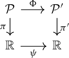
Let X and $X'$ be subsets of the vertical planes $(\mathcal {P},\pi )$ and $(\mathcal {P}',\pi ')$ respectively. We say that X and $X'$ are vertically equivalent, denoted by $X\approx _v X'$, if there exist orientation preserving homeomorphisms $\Phi : \mathcal {P} \rightarrow \mathcal {P}'$ and $\psi : \mathbb {R}\rightarrow \mathbb {R}$ such that $\Phi (X) = X'$ and the following diagram is commutative:

In the sequel we will apply the previous definition to situations when X and $X'$ are either domains of finite type in the sense of Definition 2.7 or transversal graphs in the sense of Definition 2.15.

Proposition 2.29

Let $\mathcal {D}$ and $\mathcal {D}'$ be compact connected domains of finite type in vertical planes, with Poincaré–Reeb graphs G and $G'$. Assume that both are generic in the sense of Definition 2.19. Then:

$$\begin{aligned}\mathcal {D} \approx _v \mathcal {D}' \iff G \approx _v G'.\end{aligned}$$

Before giving the proof of Proposition 2.29, let us make some remarks:

• Denote $\mathcal {C} = \partial \mathcal {D}$ and $\mathcal {C}' = \partial \mathcal {D}'$. We have $\Phi (\mathcal {C}) = \mathcal {C}'$.

• $\Phi$ sends the topological critical points $\{P_i\}$ of $\mathcal {C}$ bijectively to the topological critical points $\{P_i'\}$ of $\mathcal {C}'$. In fact, such a critical point may be geometrically characterized by the local behavior of $\mathcal {D}$ relative to the vertical line through this point. A point P is a topological critical point of $\pi _{|\mathcal {C}}$, if and only if the intersection of $\mathcal {D}$ with the vertical line $\ell$ through P is a point in a neighborhood of P, or a segment such that P is in the interior of the segment. The homeomorphism $\Phi$ sends the vertical line $\ell$ to a vertical line $\ell '$ and $\mathcal {D}$ to $\mathcal {D}'$, hence $P'=\Phi (P)$ is a topological critical point of $\pi _{|\mathcal {C}'}$.

• The equivalence preserves the $\pi$-order of the critical points: if $\mathcal {D} \approx _v \mathcal {D}'$, and if $P_i$, $P_j$ are critical points of $\pi _{|\mathcal {C}}$ with $\pi (P_i) < \pi (P_j)$ then the corresponding critical points of $\pi _{|\mathcal {C}'}$, $P'_i:=\Phi (P_i)$, $P'_j:=\Phi (P_j)$ verify $\pi '(P_i') < \pi '(P_j')$. This comes from the assumption that the homeomorphisms $\Phi$ and $\psi$ involved in Definition 2.28 are orientation preserving.

Example 2.30

Consider the canonical affine vertical plane $(\mathbb {R}^2, x)$ in the sense of Definition 2.3. Then the vertical equivalence preserves the x-order, that is to say, if $x(P_i) < x(P_j)$ then $x(P_i') < x(P_j')$. Notice that the y-order of the critical points may not be preserved. However $\Phi$ preserves the orientation on each vertical line, i.e. $y \mapsto \Phi (x_0,y)$ is a strictly increasing function.

Example 2.31

Consider again the canonical affine vertical plane $(\mathbb {R}^2, x)$ and a generic algebraic domain $\mathcal {D}$ in it, homeomorphic to a disc. Denote $\mathcal {C}=\partial \mathcal {D}$. It is homeomorphic to a circle. Then the set of critical points of $\pi |_{\mathcal {C}}$ (which are the same as the topological critical points, by the genericity assumption) yields a permutation. To explain that, we will define two total orders on the set of critical points. The first order enumerates $\{P_i\}$ in a circular manner following $\mathcal {C}$, obtained by following the curve, starting with the point with the smallest x coordinate, the curve being oriented as the boundary of $\mathcal {D}$. The second order is obtained by ordering the abscissas $x(P_i)$ using the standard order relation on $\mathbb {R}$. Now, as explained by Knuth (see [8, page 17], [23, Definition 4.21], [21, Sect. 1]), two total order relations on a finite set give rise to a permutation $\sigma$: in our case, $\sigma (i)$ is the rank of $x(P_i)$ in the ordered list of all abscissa. The vertical equivalence preserves the permutation: if $\mathcal {D} \approx _v \mathcal {D}'$ then $\sigma =\sigma '$. However, the reverse implication could be false, as shown in the Fig. 12 which shows two generic real algebraic domains homeomorphic to discs with the same permutation $\left( {\begin{matrix} 1 &{} 2 &{} 3 &{} 4 &{} 5 &{} 6 \\ 1 &{} 5 &{} 3 &{} 6 &{} 2 &{} 4 \end{matrix}}\right)$, but which are not vertically equivalent, as may be seen by considering their Poincaré-Reeb trees.

Fig. 12

Two non-vertically equivalent real algebraic domains with the same permutation

Example 2.31 shows that the permutations are not complete invariants of generic domains of finite type homeomorphic to disks, under vertical equivalence. However, by Proposition 2.29, the Poincaré–Reeb graphs is a complete invariant for the vertical equivalence.

Proof of Proposition 2.29

 

• $\Rightarrow$. Suppose $\mathcal {D}\approx _v \mathcal {D}'$ and let $\Phi : \mathcal {P}\rightarrow \mathcal {P}'$ be a homeomorphism realizing this equivalence through a commutative diagram

  

  By definition, $\Phi$ preserves the vertical foliations, hence is compatible with the vertical equivalence relations $\sim _{\mathcal {D}}$ and $\sim _{\mathcal {D}'}$ of Definition 2.11. Therefore it induces a homeomorphism $\tilde{\Phi }: \tilde{\mathcal {P}} \rightarrow \tilde{\mathcal {P}}'$ from the $\mathcal {D}$-collapse of $\mathcal {P}$ to the $\mathcal {D}'$-collapse of $\mathcal {P}'$, sending $G = \mathcal {D}/{\sim }$ to $G'=\mathcal {D}'/{\sim }$. This homeomorphism gets naturally included in a commutative diagram

  

  Therefore, by Definition 2.28, $G \approx _v G'$.

• $\Leftarrow$. The keypoint is to reconstruct the topology of a generic domain of finite type $\mathcal {D}$ homeomorphic to a disk (and of its boundary $\mathcal {C}$) from its Poincaré–Reeb graph G. To this end, one may construct a kind of tubular neighborhood $\overline{\mathcal {D}}$ of G, obtained by thickening it using vertical segments (see Fig. 13). Then $\overline{\mathcal {D}}$ is vertically equivalent to $\mathcal {D}$. Now suppose that $G \approx _v G'$ and let $\tilde{\Phi }: \tilde{\mathcal {P}} \rightarrow \tilde{\mathcal {P}}'$ be a homeomorphism inducing this equivalence. This homeomorphism induces also a vertical equivalence of convenient such thickenings, hence yields the equivalence $\mathcal {D} \approx _v \mathcal {D}'$.

$\square$

Fig. 13

Thickening in the neighborhood of an exterior vertex (left) and of an interior vertex (right)

The combinatorial types of generic transversal graphs can be realized by special types of graphs with smooth edges in the canonical affine vertical plane $(\mathbb {R}^2, x:\mathbb {R}^2\rightarrow \mathbb {R})$:

Proposition 2.32

Any generic transversal graph in a vertical plane is vertically equivalent to a graph in the canonical affine vertical plane, whose edges are moreover smooth and smoothly transversal to the vertical lines.

We leave the proof of this proposition to the reader.

Remark 2.33

We said at the beginning of this subsection that we introduced vertical equivalence as a way to capture the combinatorial aspects of subsets of vertical planes. It is easy to construct a combinatorial object (that is, a structure on a finite set) which encodes the combinatorial type of a generic transversal graph. For instance, given such a graph G, one may number its vertices from 1 to n in the order of the values of the vertical projection $\pi$. Then, for each edge $\alpha$ of G, one may remember both its end points $a < b$ and, for each number $c \in \{a+1, \dots , b-1\}$, whether $\alpha$ passes below or above the vertex numbered c.

3 Algebraic realization in the compact connected case

In this section we give the main result of the paper, Theorem 3.5: given a compact connected generic transversal graph G in a vertical plane (see Definition 2.15), we prove that there exists a compact algebraic domain in the canonical affine vertical plane whose Poincaré–Reeb graph is vertically equivalent to G. We will prove a variant of Theorem 3.5 for non-compact graphs in the next section (Theorem 4.6).

Using the canonical orientation of the target $\mathbb {R}$ of the vertical projection, one may distinguish two kinds of interior and exterior vertices of the graph G (see Fig. 14).

Fig. 14

The two kinds of interior vertices (on the left) and of exterior vertices (on the right)

Our strategy of proof of Theorem 3.5 is as follows:

• we realize the generic transversal graph G as a Poincaré–Reeb graph of a finite type domain defined by a smooth function;

• we present a Weierstrass-type theorem that approximates any smooth function by a polynomial function;

• we adapt this Weierstrass-type theorem in order to control vertical tangents, and we realize G as the Poincaré–Reeb graph of a generic finite type algebraic domain.

3.1 Smooth realization

First, we construct a smooth function f that realizes a given generic transversal graph.

Proposition 3.1

Let G be a compact connected generic transversal graph. There exists a $\mathcal {C}^{\infty }$ function $f: \mathbb {R}^2 \rightarrow \mathbb {R}$ such that the curve $\mathcal {C} = (f=0)$ does not contain critical points of f and is the boundary of a domain of finite type whose Poincaré–Reeb graph in the canonical vertical plane $(\mathbb {R}^2, x)$ is vertically equivalent to G.

Fig. 15

A generic compact transversal graph (left) and a local smooth realization (right)

Proof

The idea is to construct first the curve $\mathcal {C}$, then the function f. We construct $\mathcal {C}$ by interpolating between local constructions in the neighborhoods of the vertices of G (see Fig. 15). Let us be more explicit. We may assume, up to performing a vertical equivalence, that G is a graph with smooth compact edges in the canonical affine vertical plane $(\mathbb {R}^2, x)$, whose edges are moreover smoothly transversal to the verticals (see Proposition 2.32). Let $\varepsilon > 0$ be fixed. Then, one may construct $\mathcal {C}$ verifying the following properties:

• $\mathcal {C}$ is compact;

• $\mathcal {C} \subset N(G,\varepsilon )$: the curve is contained in the $\varepsilon$-neighborhood of G;

• $\mathcal {C}$ has only one vertical tangent associated to each vertex of G;

• all these tangents are ordered in the same way as the vertices of G.

Note that this last condition is automatic once $\varepsilon$ is chosen less than half the minimal absolute value $| x(P_i) - x(P_j)|$, where $P_i$ and $P_j$ are distinct vertices of G.

Once $\mathcal {C}$ is fixed, one may construct f by following the steps:

• Bicolor the complement $\mathbb {R}^2 \setminus \mathcal {C}$ of $\mathcal {C}$ using the numbers $\pm 1$, such that neighboring connected components have distinct associated numbers. Denote by $\sigma : \mathbb {R}^2 \setminus \mathcal {C} \rightarrow \mathbb {R}$ the resulting function.

• Choose pairwise distinct annular neighborhoods $N_i$ of the connected components $\mathcal {C}_i$ of $\mathcal {C}$, and diffeomorphisms $\phi _i: N_i \simeq \mathcal {C}_i \times (-1, 1)$ such that $p_2 \circ \phi _i$ (the composition of the second projection $p_2: \mathcal {C}_i \times (-1, 1) \rightarrow (-1, 1)$ and of $\phi _i$) has on the complement of $\mathcal {C}_i$ the same sign as $\sigma$.

• For each connected component $S_j$ of $\mathbb {R}^2 \setminus \mathcal {C}$, consider the open set $U_j \subset S_j$ obtained as the complement of the union of annuli of the form $\phi _i^{-1}(\mathcal {C}_i \times [-1/2, 1/2])$. Then consider the restriction $\sigma _j: U_j \rightarrow \mathbb {R}$ of $\sigma$ to $U_j$.

• Fix a smooth partition of unity on $\mathbb {R}$ subordinate to the locally finite open covering consisting of the annuli $N_i$ and the sets $U_j$. Then glue the smooth functions $p_2 \circ \phi _i: N_i \rightarrow \mathbb {R}$ and $\sigma _j: U_j \rightarrow \mathbb {R}$ using it.

• The resulting function f satisfies the desired properties.

$\square$

3.2 A Weierstrass-type approximation theorem

Let us first recall the following classical result:

Theorem 3.2

(Stone–Weierstrass theorem, [24]). Let X be a compact Hausdorff space. Let C(X) be the Banach $\mathbb {R}$-algebra of continuous functions from X to $\mathbb {R}$ endowed with the norm $\Vert \cdot \Vert _\infty$. Let $A \subset C(X)$ be such that:

• A is a sub-algebra of C(X),

• A separates points (that is, for each $x,y \in X$ with $x\ne y$ there exists $f \in A$ such that $f(x) \ne f(y)$),

• for each $x \in X$, there exists $f \in A$ such that $f(x) \ne 0$.

Then A is dense in C(X) relative to the norm $\Vert \cdot \Vert _\infty$.

We will only use the previous theorem through the following corollary:

Corollary 3.3

Let $f: \mathbb {R}^2 \rightarrow \mathbb {R}$ be a continuous map and $a,b\in \mathbb {R}, a<b$. For each $\varepsilon >0$, there exists a polynomial $p \in \mathbb {R}[x,y]$ such that:

$$\begin{aligned}\forall (x,y) \in [a,b]\times [a,b] \quad \big | f(x,y) - p(x,y) \big | < \varepsilon \end{aligned}$$

Proof

We apply Theorem 3.2 with $X = [a,b]\times [a,b]$, $A=\mathbb {R}[x,y]$. This set A satisfies the three conditions of Theorem 3.2 (the last one because $1_X \in A$), therefore A is dense in C(X), which implies that f can indeed be uniformly arbitrarily well approximated on X by polynomials. $\square$

Is Corollary 3.3 sufficient to answer the realization question? No! Indeed, even if it provides a polynomial p(x, y) such that $(p(x,y)=0)$ lies in a close neighborhood of $(f(x,y)=0)$, we have no control on the vertical tangents of the algebraic curve $(p=0)$, whose Poincaré–Reeb graph can therefore be more complicated than the Poincaré–Reeb graph of $(f=0)$. In the sequel we construct a polynomial p by keeping at the same time a control on the vertical tangents of a suitable level curve of it.

3.3 Algebraic realization

Proposition 3.4

Let $f: \mathbb {R}^2 \rightarrow \mathbb {R}$ be a $C^3$ function such that $\mathcal {C} = (f=0)$ is a curve which does not contain critical points of f, which has only simple vertical tangents, and is included in the interior of a compact subset K of $\mathbb {R}^2$. For each $\delta >0$, there exists a polynomial $p\in \mathbb {R}[x,y]$ such that (see Fig. 16):

• $(p=0) \cap K \subset N(f=0,\delta )$,

• for each point $P_0 \in (f=0)$ where $(f=0)$ has a vertical tangent, there exists a unique $Q_0 \in (p=0)$ in the disc $N(P_0,\delta )$ centered at $P_0$ and of radius $\delta$ such that $(p=0)$ has also a vertical tangency at $Q_0$,

• $(p=0) \cap K$ has no vertical tangent except at the former points.

Fig. 16

Algebraic realization

We prove this proposition in Sect. 3.4 below.

By taking the numbers $\varepsilon > 0$ and $\delta > 0$ appearing in Propositions 3.1 and 3.4 sufficiently small, we get:

Theorem 3.5

Any compact connected generic transversal graph can be realized as the Poincaré–Reeb graph of a connected algebraic domain of finite type.

Proof of the theorem

Starting with a compact connected transversal generic graph G, it can be realized by a smooth function f (Proposition 3.1), which in turn can be replaced by a polynomial map p (Proposition 3.4).

The referees ask:

Question

Is it possible to estimate the degree of a polynomial defining the algebraic domain in term of the combinatorics of the graph G?

A referee suggested to use a degree effective version of the $\mathcal {C}^k$ Weierstrass polynomial approximation theorem, as in [1, Theorem 2]. Furthermore, in [13], the authors construct an algebraic hypersurface that approximates a smooth compact hypersurface with a control of its minimal degree in terms of geometric data of the hypersurface.

3.4 Proof of Proposition 3.4

3.4.1 Compact support

Let $M>0$ such that $(f=0) \subset [-(M-1),M-1]^2$ (remember that $(f=0)$ is assumed to be included in a compact set). We replace the function f by a function g with compact support. More precisely, let $g: \mathbb {R}^2 \rightarrow \mathbb {R}$ be a function such that:

• g is $\mathcal {C}^3$,

• $f=g$ on $[-(M-1),M-1]^2$,

• $g=0$ outside $(-M,M)^2$,

• g does not vanish in the intermediate zone hatched area of Fig. 17.

Fig. 17

Compact support of g

Such a function may be constructed using an adequate partition of unity.

3.4.2 Polynomial approximation of g and f

We need a polynomial p approximating g, but also that some partial derivatives of p approximate the corresponding partial derivatives of g. This can be done by a $\mathcal {C}^k$ Weierstrass polynomial approximation. More precisely, one can use the density of polynomials in the $\mathcal {C}^k$ topology, as stated in [3, Proposition 1.3.7.]. Nevertheless, we state such a result and emphasise which partial derivatives we need to approximate.

Lemma 3.6

Let us fix $\varepsilon >0$. There exists a polynomial $p \in \mathbb {R}[x,y]$ such that, for all $(x,y) \in [-M,M]^2$:

$$\begin{aligned}{} & {} \left| p(x,y) - g(x,y) \right| \leqslant (2M)^3\varepsilon , \qquad \left| \partial _y p(x,y) - \partial _y g(x,y) \right| \leqslant (2M)^2\varepsilon ,\\{} & {} \left| \partial _x p(x,y) - \partial _x g(x,y) \right| \leqslant (2M)^2\varepsilon , \qquad \left| \partial _{y^2} p(x,y) - \partial _{y^2} g(x,y) \right| \leqslant 2M\varepsilon . \end{aligned}$$

In order to be self-contained we give a short proof, inspired by [7].

Proof

By Corollary 3.3 applied to the function $\partial _x\partial _y\partial _y g$ and to $(a,b) = (-M, M)$, there exists a polynomial $p_0 \in \mathbb {R}[x,y]$ such that: $\forall (x,y) \in [-M,M]^2$ $\big | p_0(x,y) - \partial _x\partial _y\partial _y g(x,y) \big | < \varepsilon .$ Now our polynomial $p \in \mathbb {R}[x,y]$ is defined by a triple integration:

$$\begin{aligned}p(x,y) = \int _{-M}^{x} \int _{-M}^{y} \int _{-M}^{y} p_0(u,v) \, dv \,dv\, du.\end{aligned}$$

We start by proving the last inequality. By Fubini theorem: $\partial _{y^2} p(x,y){=} \int _{-M}^{x} p_0(u,y) \, du.$ Therefore:

$$\begin{aligned} \left| \partial _{y^2} p(x,y) - \partial _{y^2} g(x,y) \right| = \left| \int _{-M}^{x} \big (p_0(u,y) - \partial _x\partial _{y^2} g(u,y)\big )\, du \right| \leqslant \left| \int _{-M}^{x} \varepsilon \,du \right| \leqslant 2M\varepsilon . \end{aligned}$$

The first equality is a consequence of the fact that: $\int _{-M}^{x}\partial _x\partial _{y^2} g(u,y)\, du = \partial _{y^2} g(x,y) - c(y)$ where $c(y) = \partial _{y^2} g(-M,y)$. As g vanishes outside $(-M,M)^2$, for those points we have $\partial _{y^2} g(x,y)=0$ so that $c(y)=0$. The inequality following it results from the definition of the polynomial $p_0$. By successive integrations we prove the other inequalities. $\square$

Inside the square $[-M,M]^2$ the curve $(p=0)$ defined for a sufficiently small $\varepsilon$ is in a neighborhood of $(f=0)$. However, remark that $(p=0)$ can also vanish outside the square $[-M,M]^2$.

3.4.3 The curve $(p=0)$ inside the square

Let us explain the structure of the curve $(p=0)$ around a point $P_0 \in (f=0)$ where the tangent is not vertical (recall that $f=g$ inside the square $[-(M-1),M-1]^2$) see Fig. 18.

• Fix $\delta >0$. Let $B(P_0,\delta )$ be a neighborhood of $P_0$. On this neighborhood f takes positive and negative values.

• Let $\eta >0$ and $Q_1,Q_2 \in B(P_0,\delta )$ such that $f(Q_1)>\eta$ and $f(Q_2)<-\eta$.

• We choose the $\varepsilon$ of Lemma 3.6 such that $(2M)^3 \varepsilon <\eta /2$.

• $p(Q_1)>f(Q_1)-(2M)^3\varepsilon>\eta /2>0$; a similar computation gives $p(Q_2)<0$, hence p vanishes at a point $Q_0 \in [Q_1Q_2]\subset B(P_0,\delta )$.

• Because we supposed $\partial _y f \ne 0$ in $B(P_0,\delta )$, we also have $\partial _y p \ne 0$. Hence $(p=0)$ is a smooth simple curve in $B(P_0,\delta )$ with no vertical tangent.

Fig. 18

Existence of the curve $(p=0)$

Notice that the construction of $(p=0)$ in $B(P_0,\delta )$ depends on $\varepsilon$, whose choice depends on the point $P_0$. To get a common choice of $\varepsilon$, we first cover the compact curve $(f=0)$ by a finite number of balls $B(P_0,\delta )$ and take the minimum of the $\varepsilon$ above.

3.4.4 Vertical tangency

• Let $P_0 = (x_0,y_0)$ be a point with a simple vertical tangent of $(f=0)$, see Fig. 19 that is to say:

  $$\begin{aligned}\partial _y f(x_0,y_0) = 0 \qquad \partial _x f(x_0,y_0) \ne 0 \qquad \partial _{y^2} f(x_0,y_0) \ne 0\end{aligned}$$

• For similar reasons as before, $(p=0)$ is a non-empty smooth curve passing near $P_0$.

• In the following we may suppose that the curve $(f=0$) is locally at the left of its vertical tangent, that is to say:

  $$\begin{aligned}\partial _x f(x_0,y_0) \times \partial _{y^2} f(x_0,y_0) > 0\end{aligned}$$

  An example of this behavior is given by $f(x,y):= x+y^2$ at (0, 0).

• Fix $\delta >0$. Let $B(P_0,\delta )$ be a neighborhood of $P_0$.

• $\partial _y p \sim \partial _y f$. As $\partial _y f$ vanishes at the point $P_0$ of $(f=0)$, then $\partial _y f$ takes positive and negative values near this point. Let $\eta >0$, and $Q_1 \in (f=0)$ such that $\partial _y f(Q_1)>\eta$. For a sufficiently small $\varepsilon$, there exists $R_1 \in (p=0)$ such that $\partial _y f(R_1)>\frac{2}{3}\eta$. Therefore $\partial _y p(R_1)>\frac{1}{3}\eta >0$. For a similar reason there exists $R_2\in (p=0)$ such that $\partial _y p(R_2)<0$. Then there exists $Q_0 \in (p=0) \cap B(P_0,\delta )$ such that $\partial _y p(Q_0)=0$.

• $\partial _x p \sim \partial _x f$. As $\partial _x f(P_0) \ne 0$, one has also $\partial _x p(Q_0) \ne 0$, thus p has a vertical tangent at $Q_0$.

• $\partial _{y^2} p \sim \partial _{y^2} f$ and they do not vanish near $P_0$ and $Q_0$, therefore the vertical tangent at $Q_0$ for $(p=0)$ is simple and has the same type as the vertical tangent at $P_0$ for $(f=0)$.

• Moreover as $\partial _{y^2} p \ne 0$ on $(p=0) \cap B(P_0,\delta )$, thus $\partial _y p$ vanishes only once, hence there is only one vertical tangent in this neighborhood.

Fig. 19

Vertical tangent

4 Algebraic realization in the non-compact and connected case

4.1 Domains of weakly finite type in vertical planes

We consider an algebraic domain $\mathcal {D} \subseteq \mathbb {R}^2$ in the sense of Definition 2.1, whose boundary $\mathcal {C}:= \partial \mathcal {D}$ is a connected but non-compact curve. This curve $\mathcal {C}$ is homeomorphic to a line and has two branches at infinity (the germs at infinity of the two connected components of $\mathcal {C}\setminus K$, where $K \subset \mathcal {C}$ is a non-empty compact arc). Let us suppose that these branches are in generic position w.r.t. the vertical direction: none of them has a vertical asymptote. This leads us to Definition 4.1 below, which represents a generalization of the notion of domain of finite type (see Definition 2.7), since we only ask $\pi _{|_{\mathcal {C}}}: \mathcal {C}\rightarrow \mathbb {R}$ to be proper, allowing $\pi _{|_{\mathcal {D}}}: \mathcal {D}\rightarrow \mathbb {R}$ not to be so. In turn, the genericity notion is an analog of that introduced in Definition 2.19.

Definition 4.1

Let $(\mathcal {P},\pi )$ be a vertical plane. Let $\mathcal {D}\subset \mathcal {P}$ be a closed subset homeomorphic to a surface with non-empty boundary. Denote by $\mathcal {C}$ its boundary. We say that $\mathcal {D}$ is a domain of weakly finite type in $(\mathcal {P},\pi )$ if:

• (1) the restriction $\pi _{|_{\mathcal {C}}}: \mathcal {C}\rightarrow \mathbb {R}$ is proper;

• (2) the topological critical set $\Sigma _{\text {top}} (\mathcal {C})$ is finite.

Such a domain is called generic if no two topological critical points of $\mathcal {C}$ lie on the same vertical line. A Poincaré–Reeb graph of a generic domain of weakly finite type is one of its Poincaré–Reeb graphs in the source in the sense of Sect. 2.7.

For instance, the closed upper half-plane $\mathbb {H}$ in $(\mathbb {R}^2, x)$ is a generic domain of weakly finite type (for which $\Sigma _{\text {top}} (\mathcal {C}) = \emptyset$). Its Poincaré-Reeb graphs are the sections of the restriction $x: \mathbb {H} \rightarrow \mathbb {R}$ of the vertical projection.

4.2 The combinatorics of non-compact Poincaré–Reeb graphs

Let $\mathcal {D}$ be a domain of weakly finite type in a vertical plane $(\mathcal {P}, \pi )$. When $\mathcal {C}$ is homeomorphic to a line, we distinguish three cases, depending on the position of $\mathcal {D}$ and of the branches of $\mathcal {C}$. We enrich the Poincaré–Reeb graph, by adding arrowhead vertices representing directions of escape towards infinity. Moreover, the unbounded edges are decorated with feathers oriented upward or downward, to indicate the unbounded vertical intervals contained in the domain (Figs 20, 21, 22).

Case A: One arrow

Fig. 20

Case A

In case A, the two branches of $\mathcal {C}$ are going in the same direction (to the right or to the left, as defined by the orientations of $\mathcal {P}$ and the target line $\mathbb {R}$ of $\pi$), $\mathcal {D}$ being in between. Then we get a Poincaré–Reeb graph with one arrow (and no feathers).

Case B: Two arrows

Fig. 21

Case B

In case B, the two branches have opposite directions. Then we have a Poincaré–Reeb graph with two arrows, each arrow-headed edge being decorated with feathers (above or below), indicating the non-compact vertical intervals of type $[0,+\infty [$ or $]-\infty ,0]$ contained in the domain bounded by that edge.

Case C: Three arrows

Fig. 22

Case C

In case C, where the two branches are going to the same direction but $\mathcal {D}$ is in the “exterior”, we have a graph with three arrows: two arrows with simple feathers (for the vertical intervals of type $[0,+\infty [$ or $]-\infty ,0]$) and one arrow with double feathers (for the vertical intervals of type $]-\infty ,+\infty [$).

Remark 4.2

• We can avoid the contraction of non-compact vertical intervals in the construction of the Poincaré–Reeb graph in case B and case C, in order to still have a graph G naturally embedded in an affine plane. We first define a subset $\mathcal {H} \subset \mathbb {R}^2$ that contains $\mathcal {C}$, whose boundary $\partial \mathcal {H} = H_+ \cup H_-$ is the union of two curves homeomorphic to $\mathbb {R}$, transverse to the vertical foliation (one above $\mathcal {C}$, one below $\mathcal {C}$).

  

  We change Definition 2.11, by contracting vertical intervals of $\mathcal {D} \cap \mathcal {H}$ (instead of vertical intervals of $\mathcal {D}$): $P\sim _{\mathcal {D}} Q$ if $\pi (P)=\pi (Q):=x_0$ and P and Q are on the same connected component of $\mathcal {D} \cap \mathcal {H} \cap \pi ^{-1}(x_0)$.

• The feather decoration on non-arrowheaded edges can be recovered from feathers at the other arrows and are omitted.

• The cases A and C are complementary (or dual of each other). We can pass from one to the other by considering ${\mathcal {C}}$ as the boundary of ${\mathcal {D}}$ or of $\mathbb {R}^2 \setminus {\mathcal {D}}$.

• From this point of view, case B is its own complementary case. More on such complementarities will be said later (see Sect. 5).

Proposition 4.3

Let $\mathcal {D}$ be a simply connected generic domain of weakly finite type in a vertical plane. Then its Poincaré–Reeb graph is a generic transversal binary tree.

Proof

After applying a vertical equivalence in the sense of Definition 2.28, we may assume that $\mathcal {D}$ is embedded in the canonical vertical plane $(\mathbb {R}^2, x)$.

Denote $\mathcal {C}:=\partial \mathcal {D}.$ The idea is to intersect $\mathcal {C}$ (and $\mathcal {D}$) with a sufficiently big compact convex topological disk K, to apply our previous construction for $\mathcal {D} \cap K$, then to add suitable arrows. In the Fig. 23, such a disk is represented as a Euclidean one, but one has to keep in mind that its shape may be different, for instance a rectangle, in order to achieve topological transversality between its boundary and the curve $\mathcal {C}$. $\square$

Fig. 23

Cases A, B, C (from left to right). The filled region is the compact domain of finite type $\mathcal {D}':= \mathcal {D} \cap K$. A Poincaré–Reeb graph in the source is also displayed. The Poincaré–Reeb graph of $\mathcal {D}$ is obtained by replacing each circled vertex by an arrow

First, notice that the case where $\mathcal {C}$ is compact is already known (see Propositions 2.18 and 2.25). Assume therefore that $\mathcal {C}$ is a non-compact curve. Then $\pi _{|\mathcal {C}}$ has a finite number of topological critical points. We consider a sufficiently large convex compact topological disk K that contains all these critical points. Let $\mathcal {D}':= \mathcal {D} \cap K$ and $\mathcal {C}':= \partial \mathcal {D}'$. We are then in the compact situation studied before. By Proposition 2.25, the Poincaré–Reeb graph of $\mathcal {D}'$ is a tree. We add arrows at each circled dot of Fig. 23.

We extend now the notion of vertical equivalence of transversal graphs from Definition 2.28 to enriched non-compact transversal graphs, requiring that arrowhead vertices are sent to arrowhead vertices. Then we have the following generalization of Theorem 2.29, whose proof is similar:

Proposition 4.4

Let $\mathcal {D}$, $\mathcal {D}'$ be generic simply connected domains of weakly finite type. Then:

$$\begin{aligned}\mathcal {D} \approx _v \mathcal {D}' \iff G \approx _v G'.\end{aligned}$$

4.3 Algebraic realization

We extend our realization theorem (Theorem 3.5) of generic transversal graphs as Poincaré–Reeb graphs of algebraic domains to the simply connected but non-compact case. The idea is to use the realization from the compact setting and consider the union with a line (or a parabola); finally, we take a neighboring curve.

Example 4.5

Here is an example, see Fig. 24: starting from an ellipse $(f=0)$, we consider the union with a line $(g=0)$, then the unbounded component of $(f g = \varepsilon )$ is a non-compact curve with two branches that have the shape of the ellipse on a large arc, if the sign of $\varepsilon$ is conveniently chosen.

Fig. 24

Adding two branches to an ellipse

Theorem 4.6

Let G be a connected, non-compact, generic transversal tree in a vertical plane, with at most three unbounded edges, not all on the same side (left or right), enriched with compatible arrows and feathers (like in cases A, B or C of Sect. 4.2). Let $G'$ be the compact tree obtained from G, by replacing each arrow by a sufficiently long edge with a circle vertex at the extremity (see Fig. 25). If $G'$ can be realized by a connected real algebraic curve, then G can be realized as the Poincaré–Reeb graph of a simply connected, non-compact algebraic domain in $(\mathbb {R}^2, x)$.

Fig. 25

An example of a tree G (left) and its corresponding compact tree $G'$ (right) after the edges ended with arrows have been replaced by long enough edges having circle vertices

Remark 4.7

Note that in this section we work under the additional hypothesis that the realization from the compact setting is done by a connected real algebraic curve and not by a connected component of a real algebraic curve as it was done in Theorem 3.5. We impose this hypothesis, in order not to have difficulties when taking neighboring curves (see Remark 4.10).

Proof

By hypothesis, there exists a connected real algebraic curve $\mathcal {C}:(f=0)$, $f\in \mathbb {R}[x,y]$ such that $\mathcal {C}$ realizes the newly obtained tree $G'$. In this proof we consider Poincaré–Reeb graphs in the source in the sense of Sect. 2.7, so that the graph is situated in the same plane as the connected real algebraic curve $\mathcal {C}:(f=0)$.

The key idea of the proof is to choose appropriately a non-compact algebraic curve $\mathcal {C}':(g=0)$, $g\in \mathbb {R}[x,y]$ such that when we take a neighboring level of the product of the two polynomials, say $(fg=\varepsilon )$ for a sufficiently small $\varepsilon >0$, we obtain the desired shape at infinity described by Case A, B or C. Note that the vertices of the Poincaré–Reeb graph are, by definition, transversal intersection points between the polar curve and the level curve. So a small deformation of the level curve will not change this property. Moreover, the neighboring curve must preserve the total preorder between the vertices of the tree. Since there are finitely many such vertices, we can choose $\varepsilon$ small enough to ensure this condition holds.

Let us give more details depending on the cases A, B or C.

Case A. Our goal is to realize the tree from Case A. Namely, we want to add two new non-compact branches that are unbounded in the same direction (see Fig. 26). In order to achieve this, we shall consider the graph $(g=0)$ of a parabola that is tangent to the curve $(f=0)$ in the rightmost vertex of $G'$. Next, consider the real bivariate function $fg:\mathbb {R}^2\rightarrow \mathbb {R}$. The level curve $(fg=0)$ is the union of $\mathcal {C}$ and $\mathcal {C}'.$ Finally, a neighboring curve $(fg=\varepsilon )$ realizes the tree G, for $\varepsilon \ne 0$ sufficiently small.

Fig. 26

Zoom on the construction for case A

Example 4.8

Here are the pictures of a graph $G'$ (Fig. 27) and its realization (Fig. 28).

Fig. 27

Graph G to be realized

Fig. 28

Case A: adding two new branches in the same direction

Case B. In Case B, the goal is to add two new non-compact branches, on opposite sides. First, note that in the presence of two such unbounded branches, the edges decorated by feathers (that is, those edges corresponding to the contraction of unbounded segments) form a linear graph L. The extremities of this linear subgraph are the arrowhead vertices of G which we replace by two circular vertices to define $G'$.

As before, by hypothesis we can consider a connected real algebraic plane curve $\mathcal {C}: (f=0)$ that realizes the graph $G'$. Consider a curve $(g=0)$, algebraic, homeomorphic to a line and situated just below the graph $G'$. More precisely $(g=0)$ is situated in between the linear graph L of $G'$ and the lower part of $(f=0)$ (see Figs. 29). The connected component of the neighboring curve $(fg=\varepsilon )$ for a sufficiently small $\varepsilon \ne 0$ will be the boundary of an algebraic domain that realizes the given tree G.

Fig. 29

Zoom on the construction for case B

Example 4.9

Here are the pictures of a graph $G'$ (Fig. 30) and its realization (Fig. 31).

Fig. 30

Graph G to be realized

Fig. 31

Case B: adding two new opposite branches

Note that in the above construction there exist other connected components of $(fg=\varepsilon )$, for instance in between the curves $(f=0)$ and $(g=0)$, but this is allowed by Definition 2.1: we considered the algebraic domain $\mathcal {D}$ given by $\partial \mathcal {D}=\mathcal {C},$ where $\mathcal {C} \subsetneq (fg=\varepsilon ).$

Case C. The domain considered in Case C is the complement of the algebraic domain, say $\mathcal {D}_A$, that we constructed in Case A. Namely, the graph G from Case C is realized by the domain $\mathcal {D}_C$, that is the closure of $\mathbb {R}^2{\setminus } \mathcal {D}_A.$ Note that in this case the two domains have the same boundary: $\partial \mathcal {D}_C=\partial \mathcal {D}_A=(fg=\varepsilon )$ and they are semialgebraic domains. $\square$

Remark 4.10

Our construction for Theorem 4.6 needs the graph $G'$ to be realized by a connected real algebraic curve. Theorem 3.5 only realizes $G'$ as one connected component $\mathcal {C}_1$ of a real algebraic plane curve $\mathcal {C}$ defined by $(f=0)$; this is not sufficient for our construction. For instance the oval $\mathcal {C}_1$ may be nested inside an oval $\mathcal {C}_2 \subset \mathcal {C}$; the curve $(fg=\varepsilon$) of the proof of Theorem 4.6 would no longer satisfy the requested conclusion (Fig. 32).

Fig. 32

Construction that does not satisfy the desired conclusion

5 General domains of weakly finite type

We consider the case of $\mathcal {D}$ being any real algebraic domain. Each connected component of $\mathcal {C}=\partial \mathcal {D}$ is either an oval (a component homeomorphic to a circle) or a line (in fact a component homeomorphic to an affine line). An essential question in plane real algebraic geometry is to study the relative position of these components.

5.1 Combinatorics

Let $(\mathcal {P},\pi )$ be a vertical plane and a generic domain $\mathcal {D} \subset \mathcal {P}$ of weakly finite type. The next result shows that the Poincaré–Reeb graph of $\mathcal {D}$ allows to recover the numbers of lines and ovals of $\mathcal {C} = \partial \mathcal {D}$.

Proposition 5.1

 

• The number of lines in $\mathcal {C}$ is:

  $$\begin{aligned}\#\{\text {arrows without feathers}\} + \frac{1}{2} \#\{\text {arrows with simple feathers}\}.\end{aligned}$$

• The number of ovals in $\mathcal {C}$ is:

  $$\begin{aligned}b_0(G)+b_1(G) - c\end{aligned}$$

  where $b_0(G)$ is the number of connected components of G, $b_1(G)$ is the number of independent cycles in G and c is the number of connected components of G having an arrowhead vertex.

Example 5.2

Let us consider Fig. 33. One arrowhead without feathers and (half of) two arrowheads with simple feathers, give a number of two lines. As $b_0(G)=3$, $b_1(G)=2$ and $c=2$, we see that $b_0(G)+b_1(G) - c = 3$ is indeed the number of ovals in $\mathcal {C}$.

Fig. 33

Ovals and lines and their Poincaré–Reeb graph

Fig. 34

Interior and exterior graphs of a domain of weakly finite type

Proof

For the first point we just notice that each line contributes to either an arrow without feathers or to two arrows with simple feathers.

For the second point, the proof is by induction on the number of ovals. If there are no ovals, then $b_0(G)=c$, and $b_1(G)=0$, therefore the formula is valid. Now start with a configuration $\mathcal {C} = \partial \mathcal {D}$ and add an oval that does not contain any other ovals. Let $\mathcal {C}'$ be the new curve and $G'$ its graph. Either the interior of the new oval is in $\mathcal {D}$, in which case $b_0(G')=b_0(G)$ and $b_1(G')=b_1(G)+1$, or the interior of the new oval is in $\mathcal {P} \setminus \mathcal {D}$, in which case $b_0(G')=b_0(G)+1$ and $b_1(G')=b_1(G)$. In both cases $c(G')=c(G)$. Conclusion: $b_0(G')+b_1(G') - c= (b_0(G)+b_1(G) - c) + 1$. $\square$

5.2 Interior and exterior graphs of domains of weakly finite type

Let $\mathcal {D}$ be a generic domain of weakly finite type in a vertical plane $(\mathcal {P}, \pi )$. Then the closure $\mathcal {D}^c$ of $\mathcal {P} \setminus \mathcal {D}$ in $\mathcal {P}$ is again a domain of weakly finite type, as $\partial \mathcal {D} = \partial \mathcal {D}^c$. We say that the Poincaré–Reeb graph G of $\mathcal {D}$ is the interior graph of $\mathcal {D}$ and that the Poincaré–Reeb graph $G^c$ of $\mathcal {D}^c$ is the exterior graph of $\mathcal {D}$ (Fig. 34).

In the next proposition, Poincaré-Reeb graphs are to be considered in the sense of Definition 4.1, that is, as Poincaré-Reeb graphs in the source:

Proposition 5.3

The interior graph G of a domain $\mathcal {D}$ of weakly finite type determines its exterior graph $G^c$.

Proof

The two graphs share the same non-arrowhead vertices. The local situation around a non-arrowhead vertex is in accordance to the trident rule, where an exterior vertex is replaced by an interior vertex and vice-versa (see Fig. 35). We also extend this rule to arrowhead vertices. $\square$

Fig. 35

The trident rule

Fig. 36

The trident rule applied at some vertices (here three vertices are completed)

Fig. 37

Completed exterior graph

Now we derive $G^c$ from G in two steps.

First step: make a local construction of the beginning of the edges of $G^c$ according to the trident rule (see Fig. 36).

Second step: complete each edge. It can be done in only one way up to vertical isotopies (see for instance Fig. 37).

References

Bagby, T., Bos, L., Levenberg, N.: Multivariate simultaneous approximation. Constr. Approx. 18(4), 569–577 (2002)
Basu, S., Cox, N., Percival, S.: On the Reeb spaces of definable maps. Discrete Comput. Geom. 68(2), 372–405 (2022)
De Lellis, C.: The Masterpieces of John Forbes Nash Jr. In: Holden, H., Piene, R. (eds) The Abel Prize 2013–2017. Springer, Cham, pp. 391–499 (2019)
de Silva, V., Munch, E., Patel, A.: Categorified Reeb graphs. Discrete Comput. Geom. 55(4), 854–906 (2016)
Dey, T.K., Mémoli, F., Wang, Y.: Topological analysis of nerves, Reeb spaces, mappers, and multiscale mappers. In: 33rd International Symposium on Computational Geometry, LIPIcs. Leibniz Int. Proc. Inform., vol. 77, Schloss Dagstuhl. Leibniz-Zent. Inform., Wadern, 2017, pp. Art. No. 36, 16
Edelsbrunner, H., Harer, J., Patel, A.K.: Reeb spaces of piecewise linear mappings. In: Computational Geometry (SCG’08). ACM, New York, , pp. 242–250 (2008)
Elredge, N.: Answer to “On finding polynomials that approximate a function and its derivative.” Exchange, question 555712 (2013)
Ghys, É.: A Singular Mathematical Promenade. ENS Éditions, Lyon (2017)
Hatcher, A.: Algebraic Topology. Cambridge University Press, Cambridge (2002)
Kitazawa, N.: On Reeb graphs induced from smooth functions on 3-dimensional closed manifolds with finitely many singular values. Topol. Methods Nonlinear Anal. 59(2B), 897–912 (2022)
Kitazawa, N.: On Reeb graphs induced from smooth functions on closed or open manifolds. Methods Funct. Anal. Topol. 28(2), 127–143 (2022)
Klemelä, J.: Level set tree methods. Wiley Interdiscip. Rev. Comput. Stat. 10(5), e1436 (2018)
Lerario, A., Stecconi, M.: What is the degree of a smooth hypersurface? J. Singul. 23, 205–235 (2021)
Masumoto, Y., Saeki, O.: A smooth function on a manifold with given Reeb graph. Kyushu J. Math. 65(1), 75–84 (2011)
Poincaré, H.: Papers on topology, cinquième complément à l’analysis situs, History of Mathematics, vol. 37, American Mathematical Society, Providence, RI; London Mathematical Society, London, 2010, Rendiconti del Circolo Matematico di Palermo (1884–1940), 45–110, Springer, translated and with an introduction by John Stillwell, 1904
Reeb, G.: Sur les points singuliers d’une forme de Pfaff complètement intégrable ou d’une fonction numérique. C. R. Acad. Sci. Paris 222, 847–849 (1946)
Saeki, O.: Theory of singular fibers and Reeb spaces for visualization, Topological methods in data analysis and visualization. IV, Math. Vis., Springer, Cham, pp. 3–33 (2017)
Saeki, O.: Reeb spaces of smooth functions on manifolds. Int. Math. Res. Not. IMRN (2022), no. 11, 8740–8768
Smale, S.: A Vietoris mapping theorem for homotopy. Proc. Am. Math. Soc. 8, 604–610 (1957)
Sorea, M.-Ş.: The shapes of level curves of real polynomials near strict local minima, Ph.D. thesis, Université de Lille/Laboratoire Paul Painlevé (2018)
Sorea, M.Ş.: Constructing separable Arnold snakes of Morse polynomials. Port. Math. 77(2), 219–260 (2020)
Sorea, M.Ş.: Measuring the local non-convexity of real algebraic curves. J. Symbolic Comput. 109, 482–509 (2022)
Sorea, M.Ş.: Permutations encoding the local shape of level curves of real polynomials via generic projections. Ann. Inst. Fourier (Grenoble) 72(4), 1661–1703 (2022)
Stone M.H.: The generalized Weierstrass approximation theorem. Math. Mag. 21(167–184), 237–254 (1948)
Acknowledgements
We thank the referees for their useful remarks and references, which improved the quality of our manuscript. In particular, we are grateful for the simplification of the proof of Proposition 2.24, using the Vietoris–Begel theorem [19] and for the references to the \(\mathcal {C}^k\) Weierstrass approximation theorem. We also thank Antonio Lerario for referring us to [13], for a possible approach towards estimating the degree of the real algebraic domains. This work was supported in part by the Labex CEMPI (ANR-11-LABX-0007-01) and by the ANR project LISA (ANR-17-CE40-0023-01). The first author thanks the University of Vienna for his visit at the Wolfgang Pauli Institute. M.-Ş. Sorea would like to thank Antonio Lerario for the very supportive working environment during her postdoc at SISSA, in Trieste, Italy. The authors have no competing interests to declare that are relevant to the content of this article.
Funding
Open access funding provided by Scuola Internazionale Superiore di Studi Avanzati - SISSA within the CRUI-CARE Agreement.
Author information
Authors and Affiliations
Corresponding author
Additional information
Publisher's Note
Springer Nature remains neutral with regard to jurisdictional claims in published maps and institutional affiliations.
Rights and permissions
Open Access This article is licensed under a Creative Commons Attribution 4.0 International License, which permits use, sharing, adaptation, distribution and reproduction in any medium or format, as long as you give appropriate credit to the original author(s) and the source, provide a link to the Creative Commons licence, and indicate if changes were made. The images or other third party material in this article are included in the article’s Creative Commons licence, unless indicated otherwise in a credit line to the material. If material is not included in the article’s Creative Commons licence and your intended use is not permitted by statutory regulation or exceeds the permitted use, you will need to obtain permission directly from the copyright holder. To view a copy of this licence, visit http://creativecommons.org/licenses/by/4.0/.
About this article
Cite this article
Bodin, A., Popescu-Pampu, P. & Sorea, MŞ. Poincaré–Reeb graphs of real algebraic domains. Rev Mat Complut 37, 473–507 (2024). https://doi.org/10.1007/s13163-023-00469-y
Received:
Accepted:
Published:
Issue Date:
DOI: https://doi.org/10.1007/s13163-023-00469-y