
Abstract
Vector symbolic architectures (VSA) are a viable approach for the hyperdimensional representation of symbolic data, such as documents, syntactic structures, or semantic frames. We present a rigorous mathematical framework for the representation of phrase structure trees and parse trees of context-free grammars (CFG) in Fock space, i.e. infinite-dimensional Hilbert space as being used in quantum field theory. We define a novel normal form for CFG by means of term algebras. Using a recently developed software toolbox, called FockBox, we construct Fock space representations for the trees built up by a CFG left-corner (LC) parser. We prove a universal representation theorem for CFG term algebras in Fock space and illustrate our findings through a low-dimensional principal component projection of the LC parser state. Our approach could leverage the development of VSA for explainable artificial intelligence (XAI) by means of hyperdimensional deep neural computation.
Introduction
Claude E. Shannon, the pioneer of information theory, presented in 1952 a “maze-solving machine” as one of the first proper technical cognitive systems [1].Footnote 1 It comprises a maze in form of a rectangular board partitioned into discrete cells that are partially separated by removable walls, and a magnetized “mouse” (nicknamed “Theseus”, after the ancient Greek hero) as a cognitive agent. The mouse possesses as an actuator a motorized electromagnet beneath the maze board. The magnet pulls the mouse through the maze. Sensation and memory are implemented by a circuit of relays, switching their states after encounters with a wall. In this way, Shannon technically realized a simple, non-hierarchic perception-action cycle (PAC) [2, 3], quite similar to the more sophisticated version depicted in Fig. 1 as a viable generalization of a cybernetic feedback loop.
Perception Action Cycle
In general, PAC forms the core of cognitive dynamic systems [4]. They describe the interaction of a cognitive agent with a dynamically changing world as shown in Fig. 1. The agent is equipped with sensors for the perception of its current state in the environment and with actuators allowing for active state changes. A central control prescribes goals and strategies for problem solving that could be trained by either trial-and-error learning as in Shannon’s construction, or, more generally, by reinforcement learning [4, 5].

Hierarchical bidirectional perception-action cycle (PAC) for a cognitive dynamic system after [3]. The scope of the present paper is indicated by the dashed boundary
In Shannon’s mouse-maze system, the motor (the actuator) pulls the mouse along a path until it bumps into a wall which is registered by a sensor. This perception is stored by switching a relay, subsequently avoiding the corresponding action. The behavior control prescribes a certain maze cell where the agent may find a “piece of cheese” as a goal. When the goal is eventually reached, no further action is necessary. In a first run, the mouse follows an irregular path according to a trial-and-error strategy, while building up a memory trace in the relay array. In every further run, the successfully learned path is pursued at once. However, when the operator modifies the arrangement of walls, the previously learned path becomes useless and the agent has to learn from the very beginning. Therefore, [1, p. 1238] concludes:
The maze-solver may be said to exhibit at a very primitive level the abilities to (1) solve problems by trial and error, (2) repeat the solutions without the errors, (3) add and correlate new information to a partial solution, (4) forget a solution when it is no longer applicable.
In Shannon’s seminal approach, the mouse learns by trial-and-error whenever it bumps into a wall. Its PAC comprises a simple stimulus-response loop as originally outlined in [2]. More sophisticated cognitive dynamic systems require hierarchically organized PAC such as that depicted in Fig. 1 where only two levels of analysis/synthesis and interpretation/articulation are indicated. [3] presented a multilayer PAC inspired by cortical connectivity. Additionally, both perception and actuation are characterized by bottom-up and top-down pathways, establishing a recurrent network architecture. Figure 1 reflects this by means of bidirectional connections for the prediction of subsequent states along the sensory pathway and the expectation of performed actuator movements along the motoric pathway. Finally, the PAC in Fig. 1 could be augmented by an “internal stage” as a mental model of the world [6]. Such PAC architectures are much more powerful than behavioristic stimulus-response systems and are also able to employ predictive coding strategies [7, 8], either by considering action as coding [5], or by anticipating events in the environment [9, 10].
Moreover, elaborated cognitive dynamic systems should be able to draw logical inferences and to communicate either with each other or with an external operator, respectively [11]. This requires higher levels of mental representations such as formal logics and grammars. Below we consider the symbolic representation system of language as a means of communication. In order to fulfill this function, word symbols are used as semantic representatives for the description of facts. The simplest case in which communication between two communication partners can be designed successfully is natural communication about facts in a shared direct environment. In this scenario, linguistic utterances can be placed in an environmental context so that their meaning can be determined in a truth-functional sense. In order to meet this requirement using a hierarchically organized PAC, a first information transformation of signal time series into ordered symbolic representations (analysis) and vice versa (synthesis) is required, which can be implemented using subsymbol-symbol-transducers (SST) [12]. This enables the access to the theoretical foundation of “Physical Symbol Systems” (PSS), with which—according to the “Physical Symbol Systems Hypothesis” (PSSH)—cognitive processes can henceforth be designed as information processing [13]. This includes a second information transformation from ordered symbol sequences into semantic representations (interpretation) and vice versa (articulation) as well as logical processing, with which the higher cognitive functions such as problem solving, logical reasoning or behavior control can be implemented. It should be noted that with each transformation, the information is converted into a more useful form. For example, the behavior of technical cognitive systems can be explained on the level at which logical information is available. In this study we focus on the representation of syntactic structures using vector symbolic architectures and therefore refer to the lower part of the hierarchically organized PAC in Fig. 1.
Consider, e.g., the operator’s utterance:
(note that symbols will be set in typewriter font in order to abstract from their conventional meaning in the first place). In a rather traditional PAC framework as shown in Fig. 1, the acoustic signal has firstly to be analyzed in order to obtain a symbol-like phonetic representation. For understanding its meaning, the agent has secondly to process the utterance grammatically through syntactic parsing. Finally, the syntactic representation, e.g. in form of a phrase structure tree, must be interpreted as a semantic representation which the agent can ultimately understand [14]. Depending upon such understanding, the agent can draw logical inferences and derive the appropriate behavior for controlling the actuators. In case of verbal behavior [16], the agent therefore computes an appropriate response, first as a semantic representation, that is articulated into a symbolic syntactic and phonetic form and finally synthesized as an acoustic signal. In any case, high-level representations are symbol-like and their processing is approximately rule-driven, in contrast to low-level sensation and actuation where physical signals are essentially continuous.
Cognitive dynamical systems can be coupled together through communication channels in such a way that the action of one PAC (the sender) is registered as perception by the other PAC (the receiver) [6]. Principally, there are two possibilities: The action of the sender may either perturb or modify the behavior of the receiver. Both cases can be described in the framework of interactive computation [15] where the computation of finite input strings is replaced by the processing of (principally) unbounded data streams. In the latter case of modification, the perception changes the intrinsic autonomous dynamics of the receiver, whereas in the former case of perturbation, only the actual state is transformed by means of a state space operator assigned to the perception. If perception is given as verbal behavior (B), the meaning of a perceived utterance becomes a mapping from antecedent states A to consequent states C. This so-called antecedent-behavior-consequent (ABC) schema [16] provides the fundament of dynamic semantics [17,18,19].
[17] discussed several kinds of propositional dynamic semantics. In its most simple form it codifies the ABC schema of [16] in such a way that a cognitive agent is in an epistemic state A that comprises the set of all logical propositions the agent believes to be true. Then, another agent utters a proposition B that acts on the belief state A by means of set algebraic unification, such that the consequent state C becomes the union \(C = A \cup \{B\}\). [17] further elaborated this simple scheme of dynamic semantics into different directions, including belief revision and Bayesian update semantics. Another extension, called dynamic predicate logic by [18], made dynamic semantics more compositional in the sense of traditional AI (cf. [19]). The latest developments consider internal algebraic structures of the perturbing perceptional stream [20]. Then a treatment in terms of algebraic representation theory analogous to that in quantum mechanics becomes necessary [21, 22].
Neural Networks
Perception-action cycles such as that depicted in Fig. 1 have been implemented through neural networks by several researchers [9, 10, 23]. [10] presented a neural network PAC for a robot’s visually guided reaching and grasping behavior that is inspired by the cortical organization of the human visual-motor system. The study [23] solves the reinforcement learning problem of Shannon’s mouse-maze system through an architecture of coupled feed-forward and long-short-term memory networks (LSTM, [24, 25]). In [9], a theory of event coding for PAC is neurally implemented by a recurrent network architecture that is able to anticipate effects in the environment, thereby ultimately allowing for predictive coding as well [7, 8]. Predictive coding, by contrast, has been neurally modeled by [26] through multiple timescales recurrent neural networks (MTRNN) of leaky-integrator units [27].
Also deploying neural networks in language technology became increasingly important in recent time. Beginning with hard-wired recurrent neural architectures [22, 28, 29, 30], the advent of deep learning algorithms leads to state-of-the-art language processing through recursive neural networks (RNN, [31]), through LSTM networks and through convolutional neural networks (CNN, [32, 33]), with their most recent improvements, capsule networks [34, 35]; for a survey consult [36,37,38, 39]. Particularly interesting are latest attempts of Smolensky and collaborators to train tensor product recurrent networks (TPRN, [40, 41, 42]) which are able to directly learn symbol-like representations by end-to-end training under a special quantization regularization constraint. Moreover, such networks provide an instantaneous association of linguistic input with semantic representations, thereby circumventing syntactic analysis and parsing.
Despite these impressive achievements, DNN are intrinsic black-box models, propagating input patterns through their hidden layers toward the associated output patterns. The hidden layers may have several hundred-thousands up to some billions synaptic weight parameters that are trained by regularized gradient climbing algorithms. After training, the network develops a hidden representation of the input features and the computational rules to transform them into output. Yet these representations are completely opaque and nobody can really explain how input is mapped onto output by a DNN [32].
Explainability
Therefore, following [43], the next-generation AI must be explainable, robust and trustworthy. Creating explainable AI (XAI) is an important challenge for current research [44,45,46]. For this aim, it is mandatory not only to develop new algorithms and network architectures, such as, e.g., TPRN [40,41,42], but also conceptual understanding of their formal structures. According to [47]: “A theory of explainable AI, with a formal and universally agreed definition of what explanations are, is lacking.” A first step towards this direction has been achieved by [48] who distinguish between opaque, interpretable, and comprehensive systems as follows:
Opaque systems. A system where the mechanisms mapping inputs to outputs are invisible to the user. It can be seen as an oracle that makes predictions over an input, without indicating how and why predictions are made. [...] Similarly, systems relying on genuine “black box” approaches, for which inspection of the algorithm or implementation does not give insight into the system’s actual reasoning from inputs to corresponding outputs, are classified as opaque. [48]
That is, computations carried out by an opaque system are neither understandable nor explainable. On the one hand, DNN that are “black boxes” are opaque in this sense [45]. On the other hand, linear systems such as support vector machines (SVM) appear to be interpretable:
Interpretable systems. A system where a user cannot only see, but also study and understand how inputs are mathematically mapped to outputs. This implies model transparency, and requires a level of understanding of the technical details of the mapping. [...] SVMs and other linear classifiers are interpretable insofar as data classes are defined by their location relative to decision boundaries. But the action of deep neural networks, where input features may be automatically learned and transformed through non-linearities, is unlikely to be interpretable by most users. [48]
Interestingly, [46, p. 84] pointed out that interpretability is a more “passive characteristic of a model referring to the level at which a given model makes sense for a human observer.” This contrasts with the model’s explainability, that can be regarded as an “active characteristic of a model, denoting any action or procedure taken by a model with the intent of clarifying or detailing its internal functions” to the human observer. The most important trait of an interpretable system is its transparency; and classical symbolic AI [49, 50, 51] is intrinsically transparent and hence interpretable [52]. However, interpretability usually requires expert knowledge for understanding and explanation, since their internal representations and computations are expressed in terms of formal grammars or languages [52].
Comprehensible systems. A comprehensible system emits symbols along with its output [...]. These symbols (most often words, but also visualizations, etc.) allow the user to relate properties of the inputs to their output. The user is responsible for compiling and comprehending the symbols, relying on her own implicit form of knowledge and reasoning about them. This makes comprehensibility a graded notion, with the degree of a system’s comprehensibility corresponding to the relative ease or difficulty of the compilation and comprehension. [...] Different users may have different tolerances in their comprehension: some may be willing to draw arbitrary relationships between objects while others would only be satisfied under a highly constrained set of assumptions. ([48])
Therefore, a comprehensible system could be a black box, yet producing symbolic output, a user is able to reason over. However, as has been emphasized by [45, 46], different users may belong to different audiences with different levels of individual skills or interests. Thus, the notion of comprehensibility is highly contextual.
Finally, [48, p. 7] define an explainable system as a comprehensible one that is augmented by a “reasoning engine” that is able to justify the emitted symbolic output. Explainable systems call for “confidence, safety, security, privacy, ethics, fairness and trust” [52, p. 3]. The meaning of “trust” has been circumscribed by [53, p. 211] “as a psychological state in which an agent willingly and securely becomes vulnerable, or depends on, a trustee, having taken into consideration the characteristics of the trustee.”
Vector Symbolic Architectures
Originally, in his maze solving machine, Shannon used an array of relays as the agent’s memory. This has later been termed the “learning matrix” by [54]. Learning matrices and vector symbolic architectures (VSA) provide viable interfaces between hierarchically organized symbolic data structures such as phrase structure trees or semantic representations in traditional AI technology on the one hand [49,50,51] and continuous state space approaches as required for deep neural networks on the other hand [32, 55]. Beginning with seminal studies by [56] and [57], and later pursued by [58, 59], and [60] among many others, those architectures have been dubbed VSA by [61] (cf. also [62]).
In a VSA, symbols and variables are represented as filler and role vectors of some underlying linear spaces [36, 63], respectively. When a symbol is assigned to a variable, the corresponding filler vector is bound to the corresponding role vector. Different filler-role bindings can be bundled together to form a data structure [62], such as a list, a frame, or a table of a relational data base [64]. Those structures can be recursively bound to other fillers and further bundled together to yield arbitrarily complex data structures [59]. In order to avoid the “curse of dimensionality” [49] induced by the binding process, vector symbolic architectures usually employ some data compression and subsequent clean-up algorithms restricting their memory capacity by the signal-to-noise ratio [58]. However, also loss-less VSA can be devised making use of infinite-dimensional functional representations as in quantum automata [65] or neural field architectures [66].
In recent applications, VSA have been employed for semantic spaces [63, 67], logical inferences [68,69,70], data base queries [64, 71], non-projective formal grammars [72, 73], and autoassociative memories [74, 75]. [6] developed a VSA model for cognitive representations and their induction in Shannon’s mouse-maze system.
In this study, we focus on transparent and interpretable cognitive dynamical systems that are originally described as traditional symbolic AI processors. For the sake of simplicity, we discuss context-free grammars (CFG) and push-down automata for formal languages [51]. Focussing on the dashed region in Fig. 1 , we elaborate earlier approaches for VSA language processors [22, 59, 73]. We rigorously prove a representation theorem for vector space representations of uncompressed filler-role bindings. To this end, we propose a novel normal form for CFG, allowing to express CFG parse trees as terms over a symbolic term algebra. Rule-based derivations over that algebra are then faithfully represented as transformation matrices in Fock space [76, 77]. In contrast to blackbox DNN, uncompressed VSA are therefore transparent and hence interpretable. Thus, our approach would be a first step towards the abovementioned “theory of explainable AI” [47] that could lead to future developments of new machine learning algorithms and the construction of reasoning engines [48] that are appropriate for desired audiences [45, 46].
Methods
We start from a symbolic, rule-based system that can be described in terms of formal grammar and automata theory. Specifically, we chose context-free grammars (CFG) and push-down automata as their processors here for the ease of exposition [51]. Note that an even more involved, non-projective grammar formalism [72], namely minimalist grammar [78] has been treated in [73] previously.
In the second step, we reformulate these languages through term algebras and their processing through partial functions over term algebras. We introduce a novel normal form for CFG, called term normal form, and prove that any CFG can be transformed into term normal form. Finally, we introduce a vector symbolic architecture by assigning basis vectors of a high-dimensional linear space to the respective symbols and their roles in a phrase structure tree. We propose a recursive function for mapping CFG phrase structure trees onto representation vectors in Fock space and prove a representation theorem for the partial rule-based processing functions. Finally, we present a software toolbox, FockBox, for handling Fock space VSA representations [79].
Context-Free Grammars
Consider again the simple sentence (1) as a motivating example. According to linguistic theory, sentences such as (1) exhibit a hierarchical structure, indicating a logical subject-predicate relationship, that can be illustrated by different means, e.g. through dependency graphs [72] or phrase structure trees [51]. For the sake of simplicity, we use the latter representation here, because phrase structure trees are directly related to context-free grammars and their accepting push-down automata.Footnote 2 In (1) “the mouse” appears as subject and the phrase “ate cheese” as the predicate, which is further organized into a transitive verb “ate” and its direct object “cheese”. The hierarchical structure of sentence (1) can therefore be either expressed through regular brackets, as in (2)
or, likewise as a phrase structure tree as in Fig. 2

Phrase structure tree of example sentence (1)
In Fig. 2 every internal node of the tree denotes a syntactic category: S stands for “sentence”, NP for “noun phrase”, the sentence’s subject, VP for “verbal phrase”, the predicate, D for “determiner”, N for “noun”, and V for “verb”.
The phrase structure tree Fig. 2 immediately gives rise to a context-free grammar (CFG) by interpreting every branch as a rewriting rule in Chomsky normal form [51, 81]
where one distinguishes between syntactical rules (3 – 5) and lexical rules (6 – 9), respectively. More abstractly, a CFG is given as a quadruple \(G = (T, N, \mathtt {S}, R)\), such that in our example \(T = \{ \mathtt{the}, \mathtt{mouse}, \mathtt{ate}, \mathtt{cheese} \}\) is the set of words or terminal symbols, \(N = \{ \mathtt{S}, \mathtt{NP}, \mathtt{VP}, \mathtt{D}, \mathtt{N}, \mathtt{V} \}\) is the set of categories or nonterminal symbols, \(\mathtt{S} \in N\) is the distinguished start symbol, and \(R \subset N \times (N \cup T)^*\) is a set of rules. A rule \(r = (A, \gamma ) \in R\) is usually written as a production \(r : A \rightarrow \gamma\) where \(A \in N\) denotes a category and \(\gamma \in (N \cup T)^*\) a finite string of terminals or categories of length \(n = |\gamma |\).
Context-free grammars can be processed by push-down automata [51]. Regarding psycholinguistic plausibility, the left-corner (LC) parser is particularly relevant because input-driven bottom-up and expectation-driven top-down processes are tightly intermingled with each other [82], resembling a predictive coding algorithm [8]. An LC parser possesses, such as any other push-down automaton, two memory tapes: firstly a working memory, called stack, operating in a last-in-first-out (LIFO) fashion, and secondly an input tape storing the sentence to be processed.Footnote 3 In the most simple cases, when a given CFG does not contain local ambiguities (as in (3 – 9) for our example (1)), an LC parser can work deterministically. The LC parsing algorithm operates in four different modes: i) if nothing else is possible and if the input tape is not empty, the first word of the input is shifted into the stack; ii) if the first symbol in the stack is the left corner of a syntactic rule, the first stack symbol is rewritten by a predicted category (indicated by square brackets in Table 1) followed by the left-hand side of the rule (project); iii) if a category in the stack was correctly predicted, the matching symbols are removed from the stack (complete); iv) if the input tape is empty and the stack only contains the start symbol of the grammar, the automaton moves into the accepting state; otherwise, syntactic language processing had failed. Applying the LC algorithm to our example CFG leads to the symbolic process shown in Table 1.
The left-corner parser shown in Table 1 essentially operates autonomously in modes project, complete and accept, but interactively in shift mode. Thus, we can significantly simplify the parsing process through a mapping from one intermediary automaton configuration to another one that is mediated by the interactively shifted input word perturbing the intrinsic structure building dynamics [15]. Expressing the configurations as temporary phrase structure trees yields then the symbolic computation in Fig. 3.

Interactive LC parse of the example sentence (1)
The first tree in Fig. 3, denoted \(\emptyset\), simply corresponds to the empty stack in Table 1, step 0. The second tree is generated by applying the CFG LC rules project (6) and (4) in steps 2 and 3. Accordingly, the third tree is obtained from the second one after processing steps 4 to 6, and so on.
According to our previous definitions, the states of the processor are the automaton configurations in Table 1 or the temporary phrase structure trees in Fig. 3, that are both interpretable in terms of LC parsing and language processing for an informed expert observer. Moreover, the processing steps in the last column of Table 1 and also the interactive mappings Fig. 3 are interpretable for the observer. In principle, one could augment the left-corner parser with a “reasoning engine” [48] that translates the formal language used in those symbolic representations into everyday language for any desired audience [45, 46]. The result would be something like the (syntactic) “meaning” \([\![ w ]\!]\) of a word w that can be regarded as the operator mapping a tree in Fig. 3 to its successor. This interactive interpretation of meaning is well-known in dynamic semantics [17,18,19].
Algebraic Description
In order to prepare the construction of a vector symbolic architecture (VSA) [56,57,58,59,60,61] and its representation theory in the next steps, we need an algebraically more sophisticated description. This is provided by the concept of a term algebra [81]. A term algebra is defined over a signature \(\Sigma = (F, \mathrm {rank})\) where F is a finite set of function symbols and \(\mathrm {rank}: F \rightarrow \mathbb {N}_0\) is an arity function, assigning to each symbol \(f \in F\) an integer indicating the number of arguments that f has to take.
To apply this idea to a CFG, we introduce a new kind of grammar normal form that we call term normal form in the following. A CFG \(G = (T, N, \mathtt {S}, R)\) is said to be in term normal form when for every category \(A \in N\) holds: if A is expanded through \(n\in \mathbb {N}\) rules, \(r_1 : A \rightarrow \gamma _1\) to \(r_n : A \rightarrow \gamma _n\), then \(|\gamma _1| = \ldots = |\gamma _n|\).
It can be easily demonstrated that every CFG can be transformed into a weakly equivalent CFG in term normal form, where weak equivalence means that two different grammars derive the same context-free language. A proof is presented in Appendix 6.1.
Obviously, the rules (3) – (5) of our example above are already in term normal form, simply because they are not locally ambiguous. Thus, we define a term algebra by regarding the set of variables \(V = N \cup T\) as signature with arity function \(\mathrm {rank}: V \rightarrow \mathbb {N}_0\) such that i) \(\mathrm {rank}(a) = 0\) for all \(a \in T\), i.e. terminals are nullary symbols and hence constants; ii) \(\mathrm {rank}(A) = |\gamma |\) for categories \(A \in N\), that are expanded through rules \(A \rightarrow \gamma\). Moreover, when G is given in Chomsky normal form, for all categories \(A \in N\) appearing exclusively in lexical rules \(\mathrm {rank}(A) = 1\), i.e. lexical categories (D, N, V) are unary functions, whereas \(\mathrm {rank}(A) = 2\) for all categories \(A \in N\) that appear exclusively in syntactic rules, which are hence binary functions.
For a general CFG G in term normal form, we define the term algebra \(\mathfrak {T}(G)\) inductively: i) every terminal symbol \(a \in T\) is a term, \(a \in \mathfrak {T}(G)\). ii) Let \(A \in N\) be a category with \(\mathrm {rank}(A) = k\) and let \(t_0, \dots , t_{k-1} \in \mathfrak {T}(G)\) be terms, then \(A(t_0, \dots , t_{k-1}) \in \mathfrak {T}(G)\) is a term. Additionally, we want to describe LC phrase structure trees as well. To this end, we extend the signature by the predicted categories \(P = \{ [\mathtt {N}], [\mathtt {VP}] \}\), that are interpreted as constants with \(\mathrm {rank}(C) = 0\) for \(C \in P\). The enlarged term algebra is denoted by \(\mathfrak {T}_\mathrm {LC}(G)\). We also allow for \(\emptyset \in \mathfrak {T}_\mathrm {LC}(G)\).
In the LC term algebra \(\mathfrak {T}_\mathrm {LC}(G)\), we encode the tree of step 1 in Fig. 3 (beginning with the empty tree \(t_0 = \emptyset\) in step 0) as term
because \(\mathrm {rank}(\mathtt{NP}) = 2\), \(\mathrm {rank}(\mathtt{D}) = 1\), and \(\mathrm {rank}(\mathtt{the}) = \mathrm {rank}(\mathtt{[N]}) = 0\). Likewise we obtain
as the term representation of the succeeding step 2 in Fig. 3.
Next, we define several partial functions over \(\mathfrak {T}_\mathrm {LC}(G)\) as follows [56, 83].
Here, the function \(\mathrm {cat}: \mathfrak {T}_\mathrm {LC}(G) \rightarrow N\) yields the category, i.e. the function symbol A of the term \(A(t_0, \dots , t_k) \in \mathfrak {T}_\mathrm {LC}(G)\). The functions \(\mathrm {ex}_i: \mathfrak {T}_\mathrm {LC}(G) \rightarrow \mathfrak {T}_\mathrm {LC}(G)\) for term extraction and \(\mathrm {cons}_k: N \times \mathfrak {T}_\mathrm {LC}(G)^{k + 1} \rightarrow \mathfrak {T}_\mathrm {LC}(G)\) as term constructor are defined only partially, when \(A(t_0, \dots ,t_k) \in \mathrm {Dom}(\mathrm {ex}_i)\), if \(k = \mathrm {rank}(A) - 1\) and \(i < k\), as well as \((A, t_0, \dots , t_k) \in \mathrm {Dom}(\mathrm {cons}_k)\), if \(k = \mathrm {rank}(A) - 1\).
By means of the term transformations (12 – 14) we can express the action of an incrementally and interactively shifted word \(a \in T\) that perturbs the intrinsic autonomous structure-building dynamics of a cognitive system [15] through a term operator \([\![ a ]\!] : \mathfrak {T}_\mathrm {LC}(G) \rightarrow \mathfrak {T}_\mathrm {LC}(G)\). For the transition from, e.g., LC tree 1 to LC tree 2 in Fig. 3 we obtain
The term operator \([\![ \mathtt{mouse} ]\!]\) corresponds to a computer program that sequentially extracts the category and the left subtree from the input data structure \(t_1\) and merges the results together into the output structure \(t_2\). Therefore, the (syntactic) meaning of the word “mouse” is its impact on the symbolic term algebra. Note that the function \([\![ \cdot ]\!]\) is known as the interpretation function in dynamic semantics [17,18,19]. Thus, term algebraic computation is transparent and straightforwardly interpretable [52].
Vector Symbolic Architectures
In vector symbolic architectures (VSA) [56,57,58,59,60,61] hierarchically organized complex data structures are represented as vectors in high dimensional linear spaces. The composition of these structures is achieved by two basic operations: binding and bundling. While bundling is commonly implemented as vector superposition, i.e. addition, different VSA realize binding in particular ways: originally through tensor products [56, 57], through circular convolution in reduced holographic representations (HRR) [58], through XOR spatter code [84] or through Hadamard products [62]. While HRR, spatter code, Hadamard products or a combination of tensor products with nonlinear compression [83] are lossy representations that require a clean-up module (usually an attractor neural network, cf. [60]), uncompressed tensor product representations of basis vectors are faithful, thereby allowing a transparent representation theory. It is the aim of the present study, to firstly elaborate the mathematical theory of uncompressed tensor product representations. We suggest to refer to such systems as to interpretable VSA [48] in this context.
Coming back to our linguistic example, we construct a homomorphism \(\psi : \mathfrak {T}_{\mathrm {LC}}(G) \cup N \rightarrow \mathcal {F}\) from the term algebra unified with its categories N to a vector space \(\mathcal {F}\) in such a way, that the structure of the transformations (12–14) is preserved. The resulting images \(\psi (t)\) for terms \(t \in \mathfrak {T}_\mathrm {LC}(G)\) become vector space operators, i.e. essentially matrices acting on \(\mathcal {F}\).
Again, we proceed inductively. First we map the symbols in \(\mathfrak {T}_\mathrm {LC}(G) \cup N\) onto vectors. To each atomic symbol \(s \in T \cup N \cup P\) we assign a so-called filler basis vector \(\vert s \rangle = \psi (s) \in \mathcal {F}\), calling the subspace \(\mathcal {V}_F = \mathrm {span}(\psi (T \cup N \cup P))\) the filler space. Its dimension \(n = \dim \mathcal {V}_F\) corresponds to the number of atomic symbols in \(T \cup N \cup P\), which is \(n = 13\) in our example.
Let further \(m = \max (\{ |\gamma | \,|\, (A \rightarrow \gamma ) \in R \})\) be the length of the largest production of grammar G. Then, we define \(m + 1\) so-called role vectors \(\vert i \rangle\), spanning the role space \(\mathcal {V}_R = \mathrm {span}(\{ \vert i \rangle \,|\, 0 \le i \le m \})\). Note that we employ the so-called Dirac notation from quantum mechanics that allows a coordinate-free and hence representation-independent description here [79, 85]. Then, the role \(\vert 0 \rangle\) denotes the 1st daughter node, \(\vert 1 \rangle\) the 2nd daughter and so on, until the last daughter \(\vert m - 1 \rangle\). The remaining role \(\vert m \rangle\) bounds the mother node in the phrase structure trees of grammar G. In our example, because G has Chomsky normal form, we have \(m = 2 = \dim \mathcal {V}_R - 1\) such that there are three roles for positions in a binary branching tree: left daughter \(\vert 0 \rangle\), right daughter \(\vert 1 \rangle\), and mother \(\vert 2 \rangle\). For binary trees, we also use a more intuitive symbolic notation: left daughter \(\vert / \rangle\), right daughter \(\vert {\setminus } \rangle\), and mother \(\vert {\wedge } \rangle\).
Let \(A(t_0, \dots , t_k) \in \mathfrak {T}_\mathrm {LC}(G)\) be a term. Then, we define the tensor product representation of \(A(t_0, \dots , t_k) \in \mathfrak {T}_\mathrm {LC}(G)\) in vector space \(\mathcal {F}\) recursively as follows
As a shorthand notation, we suggest the Dirac expression
Here the symbol “\(\otimes\)” refers to the (Kronecker) tensor product, mapping two vectors onto another vector, in contrast to the dyadic (outer) tensor product, which yields a matrix, hence being a vector space operator. In addition, “\(\oplus\)” denotes the (outer) direct sum that is mandatory for the superposition of vectors from spaces with different dimensionality in order to avoid interference effects.
Obviously, the (in principle) infinite recursion of the mapping \(\psi\) leads to an infinite-dimensional representation space
that is known as Fock space from quantum field theory [59, 76, 77, 86].
In quantum field theory, there is a distinguished state \(\vert \mathbf{0} \rangle \ne 0\), the vacuum state, spanning a one-dimensional subspace, the vacuum sector that is isomorphic to the underlying number field. According to (18), this sector is contained in the subspace spanned by filler and role spaces, \(\mathcal {V}_F \oplus \mathcal {V}_R\). Therefore, we could represent the empty tree in Fig. 3 by an arbitrary role; a suitable choice is the mother role \(\psi (\emptyset ) = \vert m \rangle \cong \vert \mathbf{0} \rangle\), hence symbolizing the vacuum state. Using the tensor product representation (16), we can recursively compute the images of our example terms above. For (10) we obtain
where we used the compressed Dirac notation \(\vert a \rangle \otimes \vert b \rangle = \vert a b \rangle\) in the last steps. The last line is easily interpretable in terms of phrase structure: It simply states that NP occupies the root of the tree, D appears as its immediate left daughter, the is the left daughter’s left daughter and a leave, and finally [N] is a leave bound to the right daughter of the root. Note that the Dirac kets have to be interpreted from the right to the left (reading the Arabic manner). The vector \(\vert t_1 \rangle\) belongs to a Fock subspace of dimension
where \(n = \dim (\mathcal {V}_F)\), \(m = \dim (\mathcal {V}_R)\) and p the embedding depth in the phrase structure tree step 1 of Fig. 3. This leads to \(q_1 = 172\) for \(\vert t_1 \rangle\)
Similarly, we get for (11)
where we have again utilized the more intuitive branching notation in the last line which can be straightforwardly interpreted in terms of tree addresses as depicted in Fig. 3 (step 2). Computing the dimension of the respective Fock subspace according to (20) yields \(q_2 = 523\) for \(\vert t_2 \rangle\).
In Fock space, the interactive and incremental action of a word \(a \in T\) is then represented as a matrix operator \([\![ a ]\!] _\psi : \mathcal {F} \rightarrow \mathcal {F}\). For the transition from (10) to (11) we obtain
In order to prove \(\psi\) a homomorphism, we define the following linear maps on \(\mathcal {F}\)
here, \(\,\mathbf{1}\) denotes the unit operator (i.e. the unit matrix) and the Dirac “bra” vectors \(\langle k|\) are linear forms from the dual role space \(\mathcal {V}_R^*\) that are adjoined to the role “ket” vectors \(\vert k \rangle\) such that \(\langle i|k\rangle = \delta _{ik}\) with Kronecker’s \(\delta _{ik} = 0(1)\) for \(i \ne k (i = k)\).
By means of these homomorphisms we compute the meaning of “mouse” as Fock space operator through
Therefore, \([\![ \mathtt{mouse} ]\!] _\psi\) is a holistic matrix operator instantaneously mapping the representation vector \(\vert t_1 \rangle\) of the partial phrase structure tree \(t_1\) onto the representation vector \(\vert t_2 \rangle\) of tree \(t_2\) by inserting the relevant fragments that have been extracted from the tree data structure \(t_1\) in terms of the symbolic functions in Eq. (15).
where we have expanded \(\vert \mathtt{N}(\mathtt{mouse}) \rangle\) as in (21) above. Note that the meaning of “mouse” crucially depends on the given state \(\vert t_1 \rangle\) subjected to the operator \([\![ \mathtt{mouse} ]\!] _\psi\), making meaning highly contextual. This is an important feature of dynamic semantics as well [17,18,19]. Locally, we can build the transformation matrix in analogy to Hebbian learning [87] for neural network
such that
since \(\langle t_1|t_1\rangle = 1\) for linearly independent filler and role vectors in uncompressed tensor product representations. Here, \([\![ \mathtt{mouse} ]\!] _\psi (\vert t_1 \rangle )\) is the local value of the transformation matrix at Fock space vector \(\vert t_1 \rangle\). Evaluating \([\![ \mathtt{mouse} ]\!] _\psi\) globally for all admissible arguments, yields a piecewise affine linear but overall nonlinear transformation [56].
The problem of learning such operators in a general VSA framework by end-to-end training has not been convincingly solved yet. However, the latest attempts of Smolensky and collaborators to train tensor product recurrent networks (TPRN) are a promising approach for this endeavor [40,41,42]. By contrast, neural automata have not to be trained at all since their synaptic connectivity is explicitly construed from the machine table of the underlying automaton [22].
Results
The main result of this study is a Fock space representation theorem for vector symbolic architectures of context-free grammars that follows directly from the definitions (23 – 25) and is proven in Appendix 6.2.
The tensor product representation \(\psi : \mathfrak {T}_\mathrm {LC}(G) \cup N \rightarrow \mathcal {F}\) is a homomorphism with respect to the term transformations (12 – 14). It holds
Therefore, the representation (16) mediates as an intertwiner between the matrix operators \(\mathbf{cat}\), \(\mathbf{ex}\), and \(\mathbf{cons}\) on Fock space (23 – 25) and their symbolic counterparts \(\mathrm {cat}\), \(\mathrm {ex}\), and \(\mathrm {cons}\) (12 – 14), entailing a commutative diagram. Hence, the uncompressed tensor product representation is faithful and interpretable.
For the particular example discussed above, we obtain the Fock space trajectory in Table 2.
Table 2 shows for each processing step in the first column the resulting Fock space vector in Dirac notation [79, 85] in the second column and the dimension of the hosting Fock subspace (third column). Column four relates these processing steps to the underpinning symbolic computation presented in Table 1 for the push-down recognizer and in Fig. 3 for the interactive LC tree generator.
Each Fock space vector is a unique point in a high-dimensional linear space that is instantaneously transformed by the Fock space representation operators associated to the shifted words. These matrices provide the interpretation of the meanings of those words.
In order to visualize the results of Fock space computation, we project the trajectory from Table 2 into a three-dimensional space using principal component analysis (PCA) [49]. PCA is a common method for data compression utilizing the directions of maximal variance in a cloud of data points. In our example, the data cloud is the trajectory of the VSA representations, computing the left-corner phrase structure trees of the sentence example (1). To this aim, we use FockBox,Footnote 4 a MATLAB toolbox provided by [79], for the efficient calculation of Fock space representations. The result is shown in Fig. 4 as illustration.

Principal component (PC) projection of the LC parser’s Fock space representation. Shown are the first three PCs
The trajectory is initialized by the vacuum state, translated into the origin by the PCA in Fig. 4. The point labeled “the” is the result of applying the meaning operator \([\![ \mathtt{the} ]\!] _\psi\) onto the vacuum state \(\vert {\wedge } \rangle\), which is the first Dirac vector \(\vert \mathtt{D} {\setminus } {\wedge } / \rangle \oplus \vert \mathtt{NP} {\setminus } {\wedge } \rangle \oplus \vert \mathtt{[N]} {\setminus } \rangle \oplus \vert \mathtt{the} / / \rangle\) in Table 2. From there, the processing trajectory moves into a different direction by exploiting the meaning operator \([\![ \mathtt{mouse} ]\!] _\psi\) upon the latter state, entailing \(\vert \mathtt{D} {\setminus } {\wedge } / / \rangle \oplus \vert \mathtt{NP} {\setminus } {\wedge } / \rangle \oplus \vert \mathtt{N} {\setminus } {\wedge } {\setminus } / \rangle \oplus \vert \mathtt{S} {\setminus } {\wedge } \rangle \oplus \vert \mathtt{[VP]} {\setminus } \rangle \oplus \vert \mathtt{mouse} / {\setminus } / \rangle \oplus \vert \mathtt{the} / / / \rangle\) afterwards. This illustrates the nonlinearity and contextuality of meaning operators which is further supported by the last two processing steps. In any case, even the three-dimensional compression by means of PCA is at least approximately interpretable as symbolic computation because each region in state space corresponds to one distinguished VSA representation. Similarly, the connecting transitions have an interpretation as symbol-like computations as well.
Discussion
In this article we developed a representation theory for context-free grammars and push-down automata in Fock space as an vector symbolic architecture (VSA). We presented rigorous proofs for the representations of suitable term algebras. To this end, we suggested a novel normal form for CFG allowing to express CFG parse trees as terms over a symbolic term algebra. Interactive computations such as the predictions of a left corner parser are transparently interpreted by partially recursive operators acting upon the linguistic term algebra. In order to construct a faithful representation of the term algebra in VSA Fock space, we encoded filler and role vectors by linearly independent basis vectors and employed uncompressed tensor product binding. As a result, rule-based derivations over the term algebra are then represented by transformation matrices in Fock space such that computations in VSA are transparent and hence interpretable as well.
For the implementation of rule-based symbolic computations in cognitive dynamic systems, such as neural networks, VSA provide a viable approach. We have proven that uncompressed tensor product representations are transparent and interpretable. Thus, our results contribute a formally sound basis for a future “theory of explainable AI” [47] and subsequent research and engineering. In contrast to current blackbox approaches, our method is essentially transparent and hence interpretable. Explainable AI applications could then be constructed by delivering suitable “reasoning engines” [48] and cognitive user interfaces (CUI) [88, 89] from such systems.
Conclusion
We reformulated context-free grammars (CFG) through term algebras and their processing through push-down automata by partial functions over term algebras. We introduced a novel normal form for CFG, called term normal form, and proved that any CFG in Chomsky normal form can be transformed into term normal form. Finally, we introduced a vector symbolic architecture (VSA) by assigning basis vectors of a high-dimensional linear space to the respective symbols and their roles in a phrase structure tree. We suggested a recursive function for mapping CFG phrase structure trees onto representation vectors in Fock space and proved a representation theorem for the partial rule-based processing functions. We illustrated our findings by an interactive left-corner parser and used FockBox, a freely accessible MATLAB toolbox, for the generation and visualization of Fock space VSA. Our approach directly encodes symbolic, rule-based knowledge into the hyperdimensional computing framework of VSA and can thereby supply substantial insights into the future development of explainable artificial intelligence (XAI).
Notes
See also Shannon’s instructive video demonstration at https://www.youtube.com/watch?v=vPKkXibQXGA.
The LC parser is named after the left corner of a subtree. Consider the phrase structure tree Fig. 2 where
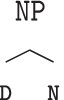
is the subtree generated by CFG rule (4). Since the article the is the first perceived word in the input stream, it is recognized as a determiner D according to CFG rule (6). Then, D is the left corner of rule (4), allowing the prediction of the yet unobserved noun N.
FockBox is available via Github at https://github.com/matthias-wolff/FockBox.

References
Shannon CE. Computers and automata. Proceedings of the Institute of Radio Engineering. 1953;41(10):1234–41.
von Uexküll J. The theory of meaning. Semiotica. 1982;4(1):25–79.
Fuster JM. Upper processing stages of the perception-action cycle. Trends in Cognitve Science. 2004;8(4):143–5.
Haykin S. Cognitive Dynamic Systems. Cambridge University Press, 2012.
Tishby N, Polani D. Information theory of decisions and actions. In: Cutsuridis V, Hussain A, Taylor JG, editors. Perception-Action Cycle: Models. Architectures, and Hardware. New York (NY): Springer; 2011. p. 601–36.
Wolff M, Huber M, Wirsching G, Römer R, beim Graben P, Schmitt I. Towards a quantum mechanical model of the inner stage of cognitive agents. In Proceedings of the 9th IEEE International Conference on Cognitive Infocommunications (CogInfoCom), 2018a. p. 000147–000152.
Friston K. Learning and inference in the brain. Neural Netw. 2003;16:1325–52.
Spratling MW. A review of predictive coding algorithms. Brain Cogn. 2017;112:92–7.
Haazebroek P, van Dantzig S, Hommel B. A computational model of perception and action for cognitive robotics. Cogn Process. 2011;12(4):355.
Cutsuridis V, Taylor JG. A cognitive control architecture for the perception-action cycle in robots and agents. Cogn Comput. 2013;5(3):383–95.
Römer R, beim Graben P, Huber M, Wolff M, Wirsching G, Schmitt I. Behavioral control of cognitive agents using database semantics and minimalist grammars. In Proceedings of the 10th IEEE International Conference on Cognitive Infocommunications (CogInfoCom), 2019. p. 73 – 78.
Wolff M, Tschöpe C, Römer R, Wirsching G. Subsymbol-Symbol-Transduktoren. In Petra Wagner, editor, Proceedings of ”Elektronische Sprachsignalverarbeitung (ESSV)”, volume 65 of Studientexte zur Sprachkommunikation, 2013. p. 197 – 204, Dresden. TUDpress.
Newell A, Simon HA. Computer science as empirical inquiry: Symbols and search. Commun ACM. 1976;19(3):113–26.
Karttunen L. Features and values. In Proceedings of the 10th International Conference on Computational Linguistics, pages 28 – 33, Stroudsburg (PA), 1984. Association for Computational Linguistics (ACL).
Wegner P. Interactive foundations of computing. Theoret Comput Sci. 1998;192:315–51.
Skinner BF. Verbal Behavior. Appleton-Century-Crofts, New York, 1957. Reprinted 2015.
Gärdenfors P. Knowledge in Flux. Cambridge (MA): Modeling the Dynamics of Epistemic States. MIT Press; 1988.
Groenendijk J, Stokhof M. Dynamic predicate logic. Linguist Philos. 1991;14(1):39–100.
Kracht M. Dynamic semantics. Linguistische Berichte, Sonderheft X:217 – 241, 2002.
beim Graben, P. Order effects in dynamic semantics. Topics in Cognitive Science. 2014;6(1):67–73.
beim Graben P. Quantum representation theory for nonlinear dynamical automata. In R. Wang, F. Gu, and E. Shen, editors, Advances in Cognitive Neurodynamics, Proceedings of the International Conference on Cognitive Neurodynamics, ICCN 2007, pages 469 – 473, Berlin, 2008. Springer.
Carmantini GS, beim Graben P, Desroches M, Rodrigues S. A modular architecture for transparent computation in recurrent neural networks. Neural Networks. 2017;85:85–105.
Kan X, Karydis K. Minimalistic neural network architectures for safe navigation of small mobile robots. In Proceedings of the 2018 IEEE International Symposium on Safety, Security, and Rescue Robotics (SSRR). 2018. p. 1–8.
Hochreiter S, Schmidhuber J. Long short-term memory. Neural Comput. 1997;9(8):1735–80.
Hupkes D, Dankers V, Mul M, Bruni E. Compositionality decomposed: How do neural networks generalise? J Art Int Res. 2020;67:757–95.
Ahmadi A, Tani J. How can a recurrent neurodynamic predictive coding model cope with fluctuation in temporal patterns? robotic experiments on imitative interaction. Neural Netw. 2017;92:3–16.
beim Graben P, Liebscher T, Kurths J. Neural and cognitive modeling with networks of leaky integrator units. In P. beim Graben, C. Zhou, M. Thiel, and J. Kurths, editors, Lectures in Supercomputational Neuroscience: Dynamics in Complex Brain Networks, Springer Complexity Series, chapter 7, pages 195 – 223. Springer, Berlin, 2008.
Chen CH, Honavar V. A neural network architecture for syntax analysis. IEEE Trans Neural Networks. 1999;10:91–114.
Pollack JB. The induction of dynamical recognizers. Mach Learn. 1991;7:227–52.
Siegelmann HT, Sontag ED. On the computational power of neural nets. J Comput Syst Sci. 1995;50(1):132–50.
Socher R, Manning CD, Ng AY. Learning continuous phrase representations and syntactic parsing with recursive neural networks. In Proceedings of the NIPS 2010 Deep Learning And Unsupervised Feature Learning Workshop, volume 2010, pages 1 – 9, 2010.
LeCun Y, Bengio Y, Hinton G. Deep learning. Nature. 2015;521(7553):436–44.
Y. N. Dauphin, A. Fan, M. Auli, and D. Grangier. Language modeling with gated convolutional networks. arXiv:1612.08083 [cs.CL], 2016.
Patrick MK, Adekoya AF, Mighty AA, Edward BY. Capsule networks – a survey. Journal of King Saud University, 2019.
Yang M, Zhao W, Chen L, Qu Q, Zhao Z, Shen Y. Investigating the transferring capability of capsule networks for text classification. Neural Netw. 2019;118:247–61.
Bengio Y, Courville A, Vincent P. Representation learning: A review and new perspectives. IEEE Trans Pattern Anal Mach Intell. 2013;35(8):1798–828.
Otter DW, Medina JR, Kalita JK. A survey of the usages of deep learning for natural language processing. IEEE Transactions on Neural Networks and Learning Systems, pages 1–21, 2020.
Goldberg Y. Neural network methods for natural language processing, volume 10 of Synthesis Lectures on Human Language Technologies. Morgan & Claypool, Williston, 2017.
Minaee S, Kalchbrenner N, Cambria E, Nikzad N, Chenaghlu M, Gao J. Deep learning based text classification: A comprehensive review. arXiv:2004.03705 [cs.CL], 2020.
Palangi H, Smolensky P, He X, Deng L. Deep learning of grammatically-interpretable representations through question-answering. arXiv:1705.08432, 2017.
Palangi H, Smolensky P, He X, Deng L. Question-answering with grammatically-interpretable representations. In Proceedings of the Thirty-Second AAAI Conference on Artificial Intelligence (AAAI-18), 2018.
Tang S, Smolensky P, de Sa VR. A simple recurrent unit with reduced tensor product representations. In Proceedings of ICLR 2020, 2019.
Marcus G. The next decade in AI: Four steps towards robust artificial intelligence. arXiv:2002.06177 [cs.AI], 2020.
Samek W, Montavon G, Vedaldi A, Hansen LK, Müller KR, editors. Explainable AI: Interpreting. Cham: Explaining and Visualizing Deep Learning. Springer; 2019.
Adadi A, Berrada M. Peeking inside the black-box: a survey on explainable artificial intelligence (XAI). IEEE Access. 2018;6:52138–60.
Arrieta AB, Díaz-Rodríguez NN, Del Ser J, Bennetot A, Tabik S, Barbado A, Garcia S, Gil-Lopez S, Molina D, Benjamins R, Chatila R, Herrera F. Explainable artificial intelligence (xai): Concepts, taxonomies, opportunities and challenges toward responsible ai. Info Fus. 2020;58:82–115.
Samek W, Müller KR. Towards explainable artificial intelligence. pages 5–22. In SamekEA19, 2019.
Doran D, Schulz S, Besold TR. What does explainable AI really mean? A new conceptualization of perspectives. arXiv:1710.00794 [cs.AI], 2017.
Russell S, Norvig P. Artificial Intelligence: A Modern Approach. Pearson, 3rd edition, 2010.
Winograd T. Understanding natural language. Cogn Psychol. 1972;3(1):1–191.
Hopcroft JE, Ullman JD. Introduction to Automata Theory, Languages, and Computation. Menlo Park, California: Addison-Wesley; 1979.
Holzinger A, Biemann C, Pattichis CS, Kell DB. What do we need to build explainable AI systems for the medical domain? arXiv:1712.09923 [cs.AI], 2017.
Došilović FK, Brčić M, Hlupić N. Explainable artificial intelligence: A survey. In Proceedings of the 41st International Convention on Information and Communication Technology, Electronics and Microelectronics (MIPRO), pages 0210–0215, 2018.
Steinbuch K, Schmitt E. Adaptive systems using learning matrices. In H. L. Oestericicher and D. R. Moore, editors, Biocybernetics in Avionics, pages 751 – 768. Gordon and Breach, New York, 1967. Reprinted in J. A. Anderson, Pellionisz and E. Rosenfeld (1990), pp. 65ff.
Schmidhuber J. Deep learning in neural networks: An overview. Neural Netw. 2015;61:85–117.
Smolensky P. Tensor product variable binding and the representation of symbolic structures in connectionist systems. Artif Intell. 1990;46(1–2):159–216.
Mizraji E. Context-dependent associations in linear distributed memories. Bull Math Biol. 1989;51(2):195–205.
Plate TA. Holographic reduced representations. IEEE Trans Neural Networks. 1995;6(3):623–41.
beim Graben P, Potthast R. Inverse problems in dynamic cognitive modeling. Chaos, 2009;19(1):015103.
Kanerva P. Hyperdimensional computing: An introduction to computing in distributed representation with high-dimensional random vectors. Cogn Comput. 2009;1(2):139–59.
Gayler RW. Vector symbolic architectures are a viable alternative for Jackendoff’s challenges. Behav Brain Sci. 2006;29:78–79.
Levy SD, Gayler R. Vector Symbolic Architectures: A new building material for artificial general intelligence. In Proceedings of the Conference on Artificial General Intelligence, pages 414–418, 2008.
Jones MN, Mewhort DJK. Representing word meaning and order information in a composite holographic lexicon. Psychol Rev. 2007;114(1):1–37.
Schmitt I, Wirsching G, Wolff M. Quantum-based modelling of database states. In: Aerts D, Khrennikov A, Melucci M, Bourama T, editors. Quantum-Like Models for Information Retrieval and Decision-Making. STEAM-H: Science, Technology, Engineering, Agriculture, Mathematics & Health. Cham: Springer; 2019. p. 115–27.
Moore C, Crutchfield JP. Quantum automata and quantum grammars. Theoret Comput Sci. 2000;237:275–306.
beim Graben P, Potthast R. Universal neural field computation. In S. Coombes, P. beim Graben, R. Potthast, and J. J. Wright, editors, Neural Fields: Theory and Applications, chapter 11, pages 299–318. Springer, Berlin, 2014.
Recchia G, Sahlgren M, Kanerva P, Jones MN. Encoding sequential information in semantic space models: Comparing holographic reduced representation and random permutation. Comput Intell Neurosci. 2015;2015:58.
Emruli B, Gayler RW, Sandin F. Analogical mapping and inference with binary spatter codes and sparse distributed memory. In Proceedings of the International Joint Conference on Neural Networks (IJCNN), pages 1–8, 2013.
Widdows D, Cohen T. Reasoning with vectors: A continuous model for fast robust inference. Logic J IGPL. 2014;23(2):141–173.
Mizraji E. Vector logic allows counterfactual virtualization by the square root of NOT. Logic J IGPL. 07 2020.
Kleyko D, Osipov E, Gayler RW. Recognizing permuted words with vector symbolic architectures: A Cambridge test for machines. Procedia Computer Science, 88:169 – 175, 2016. Proceedings of the 7th Annual International Conference on Biologically Inspired Cognitive Architectures (BICA 2016).
Kuhlmann M. Mildly non-projective dependency grammar. Comput Linguist. 2013;39(2):355–87.
beim Graben P, Gerth S. Geometric representations for minimalist grammars. J Logic Lang Info. 2012;21(4):393–432.
Gritsenko VI, Rachkovskij DA, Frolov AA, Gayler R, Kleyko D, Osipov E. Neural distributed autoassociative memories : A survey. Cybernetics and Computer Engineering Journal. 2017;188(2):5–35.
Mizraji E, Pomi A, Lin J. Improving neural models of language with input-output tensor contexts. In: Karpov A, Jokisch O, Potapova R, editors. Speech and Computer. pp. Cham: Springer; 2018. p. 430–40.
Fock V. Konfigurationsraum und zweite Quantelung. Z Phys. 1932;75(9):622–47.
Aerts D. Quantum structure in cognition. J Math Psychol. 2009;53(5):314–48.
Stabler EP. Derivational minimalism. In: Retoré C, editor. Logical Aspects of Computational Linguistics, vol. 1328. Lecture Notes in Computer Science. New York: Springer; 1997. p. 68–95.
Wolff M, Wirsching G, Huber M, beim Graben P, Römer R, and Schmitt I. A Fock space toolbox and some applications in computational cognition. In: Karpov A, Jokisch O, Potapova R, editors. Speech and Computer. pp. Cham: Springer; 2018. p. 757–67.
Seki H, Matsumura T, Fujii M, Kasami T. On multiple context-free grammars. Theoret Comput Sci. 1991;88(2):191–229.
Kracht M. The Mathematics of Language. Number 63 in Studies in Generative Grammar. Mouton de Gruyter, Berlin. 2003.
Hale JT. What a rational parser would do. Cogn Sci. 2011;35(3):399–443.
Smolensky P. Harmony in linguistic cognition. Cogn Sci. 2006;30:779–801.
Kanerva P. The binary spatter code for encoding concepts at many levels. In M. Marinaro and P. Morasso, editors, Proceedings of International Conference on Artificial Neural Networks (ICANN 1994), volume 1, pages 226 – 229, London, 1994. Springer.
Dirac PAM. A new notation for quantum mechanics. Math Proc Cambridge Philos Soc. 1939;35(3):416–8.
Smolensky P. Symbolic functions from neural computation. Philosophical Transactions of the Royal Society London, A. 2012;370(1971):3543–69.
Hebb DO. The Organization of Behavior. New York (NY): Wiley; 1949.
Young S. Cognitive user interfaces. IEEE Signal Process Mag. 2010;27(3):128–40.
Huber M, Wolff M, Meyer W, Jokisch O, Nowack K. Some design aspects of a cognitive user interface. Online J Appl Knowl Manag. 2018;6(1):15–29.
Funding
Open Access funding enabled and organized by Projekt DEAL.
Author information
Authors and Affiliations
Corresponding author
Ethics declarations
Ethical Approval
This article does not contain any studies with human participants or animals performed by any of the authors.
Conflict of Interest
The authors declare that they have no conflict of interest.
Additional information
Publisher’s Note
Springer Nature remains neutral with regard to jurisdictional claims in published maps and institutional affiliations.
Appendix
Appendix
Proof of Term Normal Form
Definition 1
A context-free grammar (CFG) is a quadruple \(G = (T, N, \mathtt {S}, R)\) with a set of terminals \(T\), a set of nonterminals \(N\), the start symbol \(\mathtt {S}\in N\) and a set of rules \(R\subseteq N\times (N \cup T)^*\). A rule \(r=(A, \gamma )\in R\) is usually written as a production \(r:A\rightarrow \gamma\).
Definition 2
According to [51] a CFG \(G = (T, N, \mathtt {S}, R)\) is said to be in Chomsky normal form iff every production \(r \in R\) is one of
with \(A\in N\), \(B, C\in N\setminus \{\mathtt {S}\}\) and \(a\in T\).
It is a known fact, that for every CFG \(G\) there is an equivalent CFG \(G'\) in Chomsky normal form [51]. It is also known that if \(G\) does not produce the empty string — absence of production (34) — then there is an equivalent CFG \(G'\) in Chomsky reduced form [51].
Definition 3
A CFG \(G = (T, N, \mathtt {S}, R)\) is said to be in Chomsky reduced form iff every production \(r\in R\) is one of
with \(A, B, C\in N\) and \(a\in T\).
By utilizing some of the construction steps for establishing Chomsky normal form from [51] we deduce
Corollary 1
For every CFG \(G\) in Chomsky reduced form there is an equivalent CFG \(G'\) in Chomsky normal form without a rule corresponding to production (34).
Proof
Let \(G\) be a CFG in Chomsky reduced form. Clearly \(G\) does not produce the empty string. The only difference to Chomsky normal form is the allowed presence of the start symbol \(\mathtt {S}\) on the right-hand side of rules in \(R\). By introducing a new start symbol \(\mathtt {S}_{0}\) and inserting rules \(\{(\mathtt {S}_{0}, \gamma )\mid \exists (\mathtt {S}, \gamma )\in R\}\) we eliminate this presence and obtain an equivalent CFG in Chomsky normal form without a production of form (34). \(\square\)
Definition 4
A CFG \(G = (T, N, \mathtt {S}, R)\) is said to be in term normal form iff \(R\subseteq N\times (N \cup T)^{+}\) and for every two rules \(r=(A, \gamma )\in R\) and \(r'=(A', \gamma ')\in R\)
holds.
We state and proof by construction:
Theorem 1
For every CFG \(G = (T, N, \mathtt {S}, R)\) not producing the empty string there is an equivalent CFG \(G'\) in term normal form.
Proof
Let \(G = (T, N, \mathtt {S}, R)\) be a CFG not producing the empty string. Let \(G' = (T, N', \mathtt {S}, R')\) be the equivalent CFG in Chomsky reduced form and \(D\subseteq N'\) be the set of all nonterminals from \(G'\) which have productions of both forms (35) and (36).
We establish term normal form by applying the following transformations to \(G'\):
-
1.
For every nonterminal \(A\in D\) let \(R_{A}''=\{(A, B \, C)\in R'\mid B,C\in N'\}\) be the rules corresponding to productions of form (35) and \(R_{A}'=\{(A, a)\in R'\mid a\in T\}\) be the rules corresponding to productions of form (36). We add
-
1.
New nonterminals \(A''\) and \(A'\),
-
2.
A new rule \((A'', B \, C)\) for every rule \((A, B \, C)\in R_{A}''\) and
-
3.
A new rule \((A', a)\) for every rule \((A, a)\in R_{A}'\).
Finally, we remove all rules \(R_{A}''\cup R_{A}'\) from \(R'\).
-
1.
-
2.
For every nonterminal \(A\in D\) let \(L_{A}=\{(X, A \, Y)\in R'\mid X, Y\in N'\}\) be the set of rules where \(A\) appears at first position on the right-hand side. For every rule \((X, A \, Y)\in L_{A}\) we add
-
1.
A new rule \((X, A'' \, Y)\) and
-
2.
A new rule \((X, A' \, Y)\).
Finally, we remove all rules \(L_{A}\) from \(R'\).
-
1.
-
3.
For every nonterminal \(A\in D\) let \(R_{A}=\{(X, Y \, A)\in R'\mid X, Y\in N'\}\) be the set of rules where \(A\) appears at second position on the right-hand side. For every rule \((X, Y \, A)\in R_{A}\) we add
-
1.
A new rule \((X, Y \, A'')\) and
-
2.
A new rule \((X, Y \, A')\).
Finally, we remove all rules \(R_{A}\) from \(R'\).
-
1.
-
4.
If \(\mathtt {S}\in D\) then we add
-
1.
A new start symbol \(\mathtt {S}_{0}\),
-
2.
A new rule \((\mathtt {S}_{0}, \mathtt {S}')\) and
-
3.
A new rule \((\mathtt {S}_{0}, \mathtt {S}'')\).
-
1.
-
5.
Finally, we remove \(D\) from \(N'\)
\(\square\)
We immediately deduce
Corollary 2
For every CFG \(G\) only producing strings of either exactly length \(1\) or at least length \(2\) there is an equivalent CFG \(G'\) in term normal form which is also in Chomsky normal form.
Proof
We handle the two cases separately.
Case 1 Let \(G\) be a CFG producing strings of exactly length \(1\). Since \(G\) does not produce the empty string there is an equivalent CFG \(G'\) in Chomsky reduced form where every rule is of form (36) and the only nonterminal being the start symbol. Obviously, \(G'\) is in Chomsky normal form and also in term normal form.
Case 2 Let \(G\) be a CFG producing strings of at least length \(2\). Since \(G\) does not produce the empty string there is an equivalent CFG in Chomsky reduced form and from Corollary 1 follows that there is an equivalent CFG in Chomsky normal form. Applying the construction from Theorem 1 to this CFG leads to a CFG \(G'\) in term normal formal. Since \(G\) does not produce strings of length \(1\) step 4 is omitted by the construction and \(G'\) stays in Chomsky normal form. \(\square\)
We also state the opposite direction.
Corollary 3
Every CFG \(G\) for which an equivalent CFG \(G'\) in Chomsky normal form exists which is also in term normal form, produces either only strings of length \(1\) or at least of length \(2\).
Proof
Let \(G = (T, N, \mathtt {S}, R)\) be a CFG in Chomsky normal form and term normal form at the same time. Clearly, \(G\) does not produce the empty string. Let \(R|_{\mathtt {S}}\subseteq R\) be the set of rules with the start symbols \(\mathtt {S}\) on the left side. Since \(G\) is in term normal form we have to consider the following two cases.
Case 1 Let \((\mathtt {S}, \gamma )\in R\) be a rule where \(\gamma \in T\). Then every rule in the set \(R|_{\mathtt {S}}\) has to be of the same form. It follows that \(G\) only produces strings of length \(1\).
Case 2 Let \((\mathtt {S}, A \, B)\in R\) be a rule with \(A,B\in \mathtt {N}\). Then every rule in the set \(R|_{\mathtt {S}}\) has to be of the same form. It follows that strings produced by \(G\) have to be at least of length \(2\). \(\square\)
We instantly deduce
Theorem 2
Those CFGs for which a Chomsky normal form in term normal exists are exactly the CFGs producing either only strings of length \(1\) or strings with at least length \(2\).
which follows directly from Corollaries 2 and 3.
Proof of Representation Theorem
The proof of the Fock space representation theorem for vector symbolic architectures follows from direct calculation using the definition of the tensor product representation (17).
Proof
\(\square\)
Rights and permissions
Open Access This article is licensed under a Creative Commons Attribution 4.0 International License, which permits use, sharing, adaptation, distribution and reproduction in any medium or format, as long as you give appropriate credit to the original author(s) and the source, provide a link to the Creative Commons licence, and indicate if changes were made. The images or other third party material in this article are included in the article's Creative Commons licence, unless indicated otherwise in a credit line to the material. If material is not included in the article's Creative Commons licence and your intended use is not permitted by statutory regulation or exceeds the permitted use, you will need to obtain permission directly from the copyright holder. To view a copy of this licence, visit http://creativecommons.org/licenses/by/4.0/.
About this article

Cite this article
Graben, P.b., Huber, M., Meyer, W. et al. Vector Symbolic Architectures for Context-Free Grammars. Cogn Comput 14, 733–748 (2022). https://doi.org/10.1007/s12559-021-09974-y
Received:
Accepted:
Published:
Issue Date:
DOI: https://doi.org/10.1007/s12559-021-09974-y