
Abstract
The Sun is magnetically active and often produces eruptive events on different energetic and temporal scales. Until recently, the upper limit of such events was unknown and believed to be roughly represented by direct instrumental observations. However, two types of extreme events were discovered recently: extreme solar energetic particle events on the multi-millennial time scale and super-flares on sun-like stars. Both discoveries imply that the Sun might rarely produce events, called extreme solar events (ESE), whose energy could be orders of magnitude greater than anything we have observed during recent decades. During the years following these discoveries, great progress has been achieved in collecting observational evidence, uncovering new events, making statistical analyses, and developing theoretical modelling. The ESE paradigm lives and is being developed. On the other hand, many outstanding questions still remain open and new ones emerge. Here we present an overview of the current state of the art and the forming paradigm of ESE from different points of view: solar physics, stellar–solar projections, cosmogenic-isotope data, modelling, historical data, as well as terrestrial, technological and societal effects of ESEs. Special focus is paid to open questions and further developments. This review is based on the joint work of the International Space Science Institute (ISSI) team #510 (2020–2022).
1 Introduction
The very title of this paper would have been written differently a decade ago when the concept of ‘extreme solar events’ (ESE) was different from what we understand now. Strong ground-level enhancement (GLE – see Sect. 2.2.1) events were considered as extreme solar events (e.g., Grechnev et al. 2008; Mironova et al. 2008). However, two very important discoveries were made in 2012 which pushed the boundaries far beyond the existing realms and led to the change of the paradigm of ESE.
One discovery was about an enormous spike in radiocarbon 14C in tree rings, specifically in high-precision measurements of Japanese cedar, dated back to the year 775 CE (Miyake et al. 2012). The spike was so strong that various exotic explanations for its origin were proposed, including an unknown supernova, a gamma-ray burst, and a cometary impact (e.g., Miyake et al. 2012; Pavlov et al. 2013; Hambaryan and Neuhäuser 2013; Liu et al. 2014). However, it was soon proven (Usoskin et al. 2013; Thomas et al. 2013; Cliver et al. 2014) that the spike was caused by a very short and extremely intense isotropic influx of energetic particles onto the Earth’s atmosphere, the most likely origin being an extreme solar-particle event (ESPE) which forms the subject of this review. The reasons for this interpretation were initially put forward by Usoskin et al. (2013) and confirmed later, as summarized below:
-
1.
Production of isotope was symmetric between northern and southern hemispheres, indicating this enhancement caused not by a point source (e.g. Güttler et al. 2015; Mekhaldi et al. 2015; Büntgen et al. 2018)
-
2.
Production was higher in polar regions, indicating magnetospheric shielding for this event and thus charged particles as its source (Uusitalo et al. 2018).
-
3.
Production was fairly consistent between different isotopes (14C, 10Be, and 36Cl), excluding gamma-rays as the event source (Usoskin et al. 2013; Mekhaldi et al. 2015; Miyake et al. 2015).
-
4.
The event (or series of consecutive events) was short, less than a few months which excludes variability of galactic cosmic rays or geomagnetic field variations (e.g., Usoskin et al. 2013; Sukhodolov et al. 2017; Büntgen et al. 2018; Uusitalo et al. 2018). This point was questioned by Zhang et al. (2022) whose results, however, cannot exclude this option (see discussion in Sect. 4.1).
-
5.
The energy spectrum of the event is totally consistent with a typical hard spectrum of a very strong solar energetic particle event (Mekhaldi et al. 2015; Paleari et al. 2022b; Koldobskiy et al. 2023)
-
6.
Such events are not unique at the centennial time scale, excluding their exotic origins (Miyake et al. 2013; Mekhaldi et al. 2015; Brehm et al. 2021; Paleari et al. 2022b; Usoskin et al. 2023).
After that, several other similar-size events have been discovered (e.g., Miyake et al. 2013; Park et al. 2017; Paleari et al. 2022a; Brehm et al. 2022), adding to the point 6 above. All these events were much stronger than the strongest directly observed solar-energetic-particle (SEP) events of the space era – see Sect. 4 and Cliver et al. (2022) for details. This approach, however, is limited to specific observables at Earth (cosmogenic isotopes in terrestrial archives) which requires formation of favourable conditions. Thus, its projection to the Sun is somewhat poorly quantified.
Another related discovery was also made in 2012 by Maehara et al. (2012) who found, using nearly four years of observations by the space-borne Kepler telescope, that Sun-like stars can produce superflares with bolometric energy at least an order of magnitude larger than that of known flares on the Sun. Although statistics of the Sun-like stars and superflares have been revisited and updated later (see more details in Sect. 3), leaving large uncertainties in the projection of stellar results on a single star, the Sun, it is generally accepted that the Sun could also, in principle, produce flares stronger than those directly observed during the recent decades.
These discoveries voided the earlier paradigm of extreme solar events, based on 20th-century data, and led to setting a new paradigm, based on indirect proxy (cosmogenic isotopes or Sun-like stars) data, that events much stronger than what we have experienced in the recent past can occasionally occur on the Sun on the centennial–millennial timescales.
This field and establishment of the new paradigm were initially developed in an erratic way, mostly by gathering more data on the extreme events, and coordination was needed to consolidate the efforts of individual research groups. Several international collaborations were formed to obtain and analyze the cosmogenic-isotope data (e.g, Usoskin et al. 2013; Mekhaldi et al. 2015; Sigl et al. 2015). In 2018, the first dedicated international workshop was organized and hosted by ISEE (Institute for Space-Earth Environmental Research) in Nagoya, Japan, where a core team of relevant world-class experts met to discuss the perspective of ESE research. The collected materials and a state-of-the-art review were published as the first textbook on the subject (Miyake et al. 2019). The teamwork continued via an International team (https://www.issibern.ch/teams/solextremevent) selected and supported by ISSI (International Space Science Institute) in Bern, Switzerland, with two team meetings held in a hybrid format in September 2021 and June 2022.
Here we present a comprehensive yet concise review of the present state of the art in the field of ESE as prepared by the international team in the framework of the ISSI team project. The paper is organized in nine topical sections. Section 2 discusses the extreme events in terms of the established Solar Physics. Projections of stellar superflares to the Sun are discussed in Sect. 3. Details of the ESPEs recorded in cosmogenic-isotope archives are presented in Sect. 4. The state of the art in modelling the cosmogenic isotope production and atmospheric transport/deposition is overviewed in Sects. 5 and 6, respectively. A description of the efforts in looking for records of extreme events in documented human history is given in Sect. 7. Terrestrial effects of extreme events are briefly discussed in Sect. 8. The paper is concluded with a short Summary in Sect. 9.
2 Solar Physics of Extreme Events
2.1 Extreme Events
In this section, we introduce extreme events produced by the Sun and describe their basic physics and occurrence probabilities.
2.1.1 Extreme SEP Events
By definition, extreme events are rare and represent the farthest tail of the distribution in the sense of strength and induced effects. As such, the classification of extreme events may change in time along with the broadening of our knowledge. For example, when speaking of SEP events, the extremes were primarily identified from direct space-borne and ground-based observations as the events with the strongest SEP peak fluxes detected in near-Earth space or atmospheric effects observable on the ground (GLEs – see Sect. 2.2.1). GLEs are caused by high-energy ions, mostly protons of energy greater than ∼400 MeV. However, the game changed in 2012 when an enormous increase of radiocarbon 14C, dated to the year 775 CE, was discovered (Miyake et al. 2012; Usoskin and Kovaltsov 2012) and soon confirmed as the greatest known SEP event which occurred in the summer of 774 CE (e.g., Usoskin et al. 2013; Sukhodolov et al. 2017; Büntgen et al. 2018; Uusitalo et al. 2018). That event was a factor of 40–100 stronger than the strongest directly observed GLE #5 of 23-Feb-1956 shown in Fig. 3 (see also Usoskin et al. 2020; Koldobskiy et al. 2022). Later, more events of similar strength (a factor of more than 20 with respect to GLE #5) have been discovered, see details in Sect. 4.
This discovery has altered the definition of extreme SEP events which are now regarded as these historically known enormous SEP events with intensities far beyond anything we have observed during the recent era of direct scientific observations. This forms a gross challenge for science because of the lack of auxiliary data, such as, e.g., solar magnetic data, solar-wind and heliospheric measurements, and theoretical models that can be validated for such extreme conditions. This paper focuses mostly on SEP events that are extreme in terms of their proton or ion fluxes. Events with significant fluxes of relativistic electrons and hard electron spectra have also been reported in the literature (e.g., Cline and McDonald 1968; Evenson et al. 1984; Dröge et al. 1989). However, we are unaware of any proxy that would make it possible to assess the severity of electron fluxes for events before the space era. The space-weather impacts of relativistic electrons is an open question.
Herewith, we overview the present state of the art and the open challenges in our understanding of the physics of extreme solar events.
2.1.2 Sources of Extreme Solar Particle Events
Extreme SEPs are associated with solar flares and coronal mass ejections (CMEs). Possible mechanisms by which these events produce energetic particles have been reviewed extensively (see, e.g., Desai and Giacalone 2016; Klein and Dalla 2017) and include acceleration during magnetic reconnection, for example via direct electric field or stochastic acceleration, and diffusive shock acceleration (DSA). For GLEs, in particular, the association with very intense flares (X-class flares) and fast CMEs is well known (Nitta et al. 2012; Belov et al. 2010; Gopalswamy et al. 2012).
There has been much debate within the scientific community about the physical mechanism responsible for the acceleration of the highest energy SEPs (e.g., protons in the ∼GeV range). The main possibilities are acceleration in the low corona during small-scale processes associated with flares and at the coronal shocks driven by CMEs. Identifying the precise acceleration mechanism of GLE protons is complicated due to the fact that in most cases GLE-associated solar events involve both an intense flare and a fast CME. It is also possible that high-energy protons may be produced by both flare-related mechanisms and the CME-driven shock within a single event, with different timings and injection properties.
A number of studies have argued that acceleration at a CME-driven shock is the dominant process in GLE events. Timing analyses, assuming scatter-free propagation and a direct magnetic connection to the particle source, place the so-called release time of GLE particles after the flare impulsive phase, at times when the CME shock was located at heights of a few solar radii (e.g., Reames 2009). Modelling of CME shock acceleration in the low corona demonstrated that the energisation of protons to GeV energies is possible (Afanasiev et al. 2018). The CME acceleration scenario readily explains the propagation of high-energy protons to Earth in the case of a not well-connected source active region (AR), because it allows for an extended source region.
Other authors have argued for a small-scale flare-related origin. For example, GLE #69, which took place on January 20th 2005, was a particularly intense and prompt event in neutron monitor (NM) data. It has been shown that it was characterised by consistent timing between particle release and impulsive flare signatures (impulsive \(\gamma \)-rays, hard-X-ray and microwave emission – e.g., Masson et al. 2009). Acceleration of protons to GLE energies over a few tens of seconds is needed for this event and it is difficult for CME acceleration to meet this requirement based on existing models (e.g., Afanasiev et al. 2018). Aschwanden (2012) concluded that GLE release times overlapped with the flare impulsive phase in 50% of the events they studied and that signatures of extended acceleration and/or particle trapping were evident in all strongly delayed cases. Within a flare scenario, propagation effects or delays due to trapping may be invoked to explain why the scatter-free release times appear delayed compared to the flare electromagnetic emissions (e.g., Masson et al. 2019). It should be noted that for most GLE events, the derived proton release times have large uncertainties due to the statistical uncertainties in NM measurements: poor statistics result in later release times.
It is important to note that only a fraction of extreme SEP events produced by the Sun can be detected on Earth as specified in Sect. 2.2.5.
2.1.3 Greatest Solar Flares
What do we know?
All discussions of the greatest observed flare must start with the “Carrington event”, denoted as SOL1859-09-01T11:20. This benchmark flare was observed in white light by two independent observers (Carrington 1859; Hodgson 1859) within a large sunspot active region near the disk centre as shown in Fig. 6 of Cliver and Keer (2012) and Figs. 2–4 of Hayakawa et al. (2019a). Coincidentally, this flare was also registered on the relatively new “self-recording magnetograph” at Kew Gardens in London (Stewart 1861) and another magnetogram in Greenwich – see Fig. 7 of Cliver and Keer (2012). As discussed at length later in this paper, the simple reported fact about the visual observation immediately implied a burst of continuum radiation with an energy of the order of \(10^{32}\text{ erg}\), likely implying a modern GOES rankingFootnote 1 above X10 (Cliver and Svalgaard 2004; Boteler 2006; Cliver and Dietrich 2013; Curto et al. 2016). The novel magnetograph observation, seen from a modern perspective, presaged the new field of “space weather”: the flare produced ionospheric disturbances both by direct XUV radiation and also by plasma interactions between the solar wind and the terrestrial magnetosphere. The year 1859 preceded the discoveries of X-rays (Röntgen 1895) and of the Kennelly-Heaviside layer (Appleton and Barnett 1926), so, of course, no clear physical interpretation could emerge at that time. These phenomena incidentally could be described as an early case of “multi-messenger astronomy.”
This space-weather juxtaposition was not observed in any of the other four white-light flares observed visually in the 19th century (Hudson 2021); the “geoeffectiveness”, therefore space-weather effects, did not seem to be reproducible. Nowadays we have many examples, though, and can recognize the Carrington event as a precursor to modern time-domain and multi-messenger astronomy. Most probably other flare events of comparable magnitude have occurred since 1859, and we discuss the modern view of the occurrence distribution function (ODF) below in Sect. 2.1.4.
To put the Carrington event into a stellar perspective, we now know that such a flare would correspond to only about an 0.1% increase in the sun-as-a-star brightness; this level of sensitivity is now a routine observational capability for stellar photometry, but a challenge that has only been met marginally in total solar irradiance (TSI) observations, the solar equivalent of stellar broad-band or bolometric photometry (Hudson and Willson 1983; Woods et al. 2006).
What flare magnitudes could be possible?
Flares have a broad distribution of magnitudes, as judged from many observables across a huge spectral domain (about 20 kHz to the GeV range). Any given observable could be taken as a proxy for the total energy released by the event, which would have a clear physical significance in terms of the magnetic field structure and dynamics. Is there maximum possible flare energy? The answer to this question could be found theoretically, in principle, but in practice, many uncertainties make this impractical at present.
Certainly, based on modern theory, more powerful flares could result from the presence of a larger amount of coronal magnetic flux. This simple consideration allowed Aulanier et al. (2013) to refer to the existing record of solar magnetism, using sunspot records as a proxy in the context of a specific model of eruptive flaring. However the correlation between sunspot areas and geoeffectiveness (e.g. Sammis et al. 2000) could be quite misleading (e.g., Fig. 12 of Hudson 2021); see also the discussion in Sect. 3.3. Certainly, sunspots and flares have no clear physical relationship, and recent observations suggest that solar active regions with great magnetic fluxes actually have diminished eruptivity (e.g. Sun et al. 2015, see also Sect. 2.2.3).
2.1.4 Distribution of Event Occurrences
Generally speaking, solar energetic phenomena often follow a power-law ODF. This pattern applies to many different observables, proxies to the total energy released by an event. If a given proxy has an extensive time history, and if its relationship with total event energy does not vary with event magnitude, it may provide clues to the behaviour of the greatest events and the possibility of extreme events.
Radio-wavelength observations have excellent sensitivity and a long history of observation, so they reflect a large dynamic range of event magnitudes. Through gyrosynchrotron radiation, they can also provide information on the most energetic particle populations. Nita et al. (2002) disentangled the very complicated observational basis of these data (wide wavelength ranges, multiple emission mechanisms, and little standardization of measurements) with the highly relevant result shown here in Fig. 1: a deviation from a simple power law at the high end. Because the radio wavelengths contain very little energy, they might not reflect total flare energies very well, but what the Figure shows is definitely suggestive.

Occurrence Distribution Function (ODF) of flare radio fluxes (Nita et al. 2002), with an artifactual deviation from the power law (slope \(\lambda \)) for the weak events, and a plausible deficit for the strong events. Cgeo is a correction factor for observer geography
The GOES soft X-ray peak fluxes, on the other hand, actually do contain a substantial fraction of the total flare energy (e.g. Emslie et al. 2012) and correlate well with chromospheric emissions such as H\(\alpha \), which dominate flare radiation energetically. The GOES/XRS soft X-ray measurements (Thomas et al. 1985; Garcia 1994; White et al. 2005) began in 1975 and now extend over two full Hale cycles. The GOES/XRS peak fluxes also follow a quite clean power law for several decades (e.g., Veronig et al. 2002). The GOES ODF power-law form also appears to fail at large magnitudes (Fig. 2), consistent with the Nita et al. (2002) result. Note that the deficit of weaker events results substantially from confusion; at high background levels weak events are harder to detect (e.g., Wheatland 2000), and some similar effect may explain the low end of the radio ODF.

Occurrence Distribution Function (ODF) of flare peak soft X-ray fluxes from the GOES 1-8 Å band, shown as a complementary cumulative distribution with N = 46,855 events above a cutoff at GOES C1 class. The red line shows a basic power law with \(dN/dS \propto S^{1.973 \pm 0.014}\) for the range M1–X3 (solid red line), in agreement with earlier determinations such as that of Aschwanden and Freeland (2012)
The rollover at the high end of the distribution (the ODF falling below the dotted red line from the power-law segment) clearly has major implications and must be considered carefully. For the cumulative distribution form of the ODF, this is a one-parameter fit, and the deviation thus calls for at least a two-parameter form. Recently Sakurai (2022) has summarized three possible empirical fitting functions for this purpose, using a tapered power law (truncated Pareto distribution), a gamma-function form, and a Weibull distribution, discarding the latter on the basis of a Kolmogorov-Smirnov test of goodness of fit. These empirical forms could of course be extrapolated to the domain of extreme events, but without theoretical support, we have no evidence that this would correctly predict their numbers.
2.2 Extreme SEP Events and Their Physics
In this section, we focus on extreme SEP events and discuss their properties and associations with flare and CME events. We focus on the physics of how energy gets partitioned. We discuss how acceleration and propagation influence solar energetic proton detection and properties at 1 AU.
2.2.1 GLE Observations
The strongest directly observed SEP events form a special class of GLEs recorded by ground-based neutron monitors (NMs) as a statistically significant enhancement of NM count rate above the background level caused by galactic cosmic rays (GCRs). The current definition (Poluianov et al. 2017) of a GLE is: “A GLE event is registered when there are near-time coincident and statistically significant enhancements of the count rates of at least two differently located neutron monitors including at least one neutron monitor near sea level and a corresponding enhancement in the proton flux measured by a space-borne instrument(s).” To be identified as a GLE, a SEP event should have a hard energy/rigidity spectrum and high peak flux so that it can initiate an atmospheric nucleonic cascade with the number of secondary cascade nucleons (mostly neutrons) at ground level being at least a few per cent that of the background GCR flux. Sometimes, GLE events are called extreme SEP events which is no longer correct.
At present, 73 GLEs have been registered and consequently numbered since 1942. The first four GLEs were detected by ground-based ionisation chambers which makes it very difficult to evaluate their quantitative parameters. GLEs since #5 in 1956 are recorded by the standard NM network and thus can be inter-compared (Koldobskiy et al. 2021). GLE events vary greatly in strength. The strongest observed GLE, GLE#5, occurred on 23-Feb-1956 and was the first GLE measured by the NM network (Usoskin et al. 2020). Count rates for GLE#5 are shown in Fig. 3 relative to the GCR background. The greatest peak increase was observed by Leeds NM and was greater than 5000% (x50 increase). The integral rigidity spectrum of GLE#5 is shown in Fig. 4 as reconstructed from the ground-based measurements (Webber et al. 2007; Usoskin et al. 2020). Such strong events happen relatively seldom – one per several decades. Weaker events are more frequent, roughly one per year, but their occurrence rate is dominated by solar activity: GLEs have a greater chance to occur around the maximum and declining phase of the solar cycle. The weakest relativistic SEP events (which are still very strong compared to ‘normal’ SEP events) form a sub-class of so-called sub-GLE events which can be only observed by high-altitude polar NMs in Antarctica (Poluianov et al. 2017). The full dataset of original data of the available NMs for the known GLEs is collected in the International GLE database (IGLED – https://gle.oulu.fi) hosted and maintained by the University of Oulu (Usoskin et al. 2015).

Records of neutron monitors (in per cent to the background count rate due to GCR) for GLE#5 of 23-Feb-1956. Panels, left to right, represent the high-, mid- and low-latitude neutron monitors, respectively. Data and NM notations are from the IGLED (https://gle.oulu.fi). Plot is modified after Usoskin et al. (2020)

Energy/rigidity spectra and anisotropy of GLE-producing particles are typically reconstructed by inversion techniques from a dataset of records of ground-based NMs (e.g., Mishev and Usoskin 2016).
2.2.2 Correlations Between Properties of SEPs and of Flares/CMEs
A large body of literature exists on the analysis of correlations between the properties of SEPs and those of flares/CMEs that energised them. Often the degree of correlation has been characterised via the Pearson correlation coefficient \(C\). These studies are important for extreme events because they can provide information on the typical magnitude of the solar events associated with the largest SEP fluxes. More generally, better/worse correlations with a particular type of solar event (flare/CME) have been used in the literature to make inferences on the possible acceleration mechanisms of SEPs, although the presence of a correlation does not imply causality.
The SEP peak intensity, \(I_{\mathrm{SEP}}\), is broadly correlated with the GOES Soft-X-Ray (SXR) peak intensity, \(I_{\mathrm{fl}}\), of the solar flare associated with the event (e.g., Papaioannou et al. 2016). Consistent with this trend, most GLE events follow very intense X-class flares. The value of the correlation coefficient for \(I_{\mathrm{SEP}}\) vs \(I_{\mathrm{fl}}\) depends on SEP energy, with \(C\) increasing with particle energy (Dierckxsens et al. 2015).
Kahler et al. (1984) was the first to identify a correlation between SEP peak intensities and the plane-of-the-sky speed of the associated CMEs, \(v_{\mathrm{CME}}\), obtained from coronagraph data, with faster CMEs tending to produce more intense SEP events. Since the 1980s, the relationship between these two properties has been studied extensively by a number of authors (e.g., Dierckxsens et al. 2015; Papaioannou et al. 2016). The value of the correlation coefficient for \(I_{\mathrm{SEP}}\) vs \(v_{\mathrm{CME}}\) was found to decrease with particle energy (Dierckxsens et al. 2015).
In the correlation of \(I_{\mathrm{SEP}}\) with both \(I_{\mathrm{fl}}\) and \(v_{\mathrm{CME}}\) there is a significant scatter so that the SEP peak intensity spans many orders of magnitude for a given CME speed or SXR flare peak.
Generally, analyses of correlations have been carried out at proton energies smaller than 100 MeV, due to the relative scarcity of SEP data at higher energies. Recently Waterfall et al. (2023) analysed proton data at energy >300 MeV using GOES/HEPAD data. Figure 5 shows the correlations with flare peak intensities that they obtained for SEP fluence (top panels) and SEP peak intensity (bottom panels) in three energy channels. The corresponding plot for correlations with CME speeds (see Fig. 7 of Waterfall et al. 2023) shows significantly less correlation than that observed at lower SEP energies.

SEP fluence (top panels) and peak intensity (bottom panels) versus GOES SXR flare peak intensity for three high energy proton channels from GOES HEPAD (reproduced from Waterfall et al. 2023)
2.2.3 CME-Less Flares and “Stealth” CMEs
By “flare” we refer to the processes involved in basic electromagnetic radiation signatures, such as the broad-band white light from the Carrington flare and nowadays H\(\alpha \) and soft X-rays (the GOES data, for example). Often there are also ejecta of various kinds (H\(\alpha \) surges and sprays; CMEs), often closely linked in the time domain to the flare emissions. The initial acceleration of CME mass strongly tends to have a close association with the impulsive phase of its associated flare (Zhang et al. 2001; Temmer et al. 2008). Other than this timing relationship, no simple correlation between flare and CME physical parameters seems to exist, although there is a definite tendency for eruptivity to increase with flare magnitude at least up to the GOES X-class range (Yashiro et al. 2005).
The lack of correlation in extensive parameters is strikingly clear in the case of “CMEless” flares, a term normally referring to the occurrence of a major (GOES X class) flares without any discernible CME occurrence (Gopalswamy et al. 2009). This seems to be a departure from the interesting concept of the “big flare syndrome” (Kahler 1982). Well-known examples of this behaviour occurred in the enormous region AR 12192 in October 2014, which had several “confined” (no CME) and yet powerful (X-class) flares. Such behaviour suggests that eruptivity, at the most energetic end of the scale, may diminish if the active region contains too much magnetic flux (Sun et al. 2015). This behaviour is not well-documented at present but may well relate to event ODFs on the Sun or Sun-like stars, to be discussed further below.
Finally, we note the presence of eruptive events at the opposite corner of the flare/CME energy distribution: the so-called “stealth CMEs” (Robbrecht et al. 2009). We identify these with filament eruptions in the quiet Sun, sometimes in the polar crown, and with other names such as “Hyder flares” or “disparitions brusques” leading to flare brightening, with the possible physical mechanism of “infall/impact” in which gravitational potential energy may drive chromospheric brightening (Hyder 1967). These events may have major CMEs but with only minor – perhaps undetectable – low-coronal disturbances.
2.2.4 Event Energy Partition
A flare/CME disturbance needs to be understood primarily in terms of the magnetic field involved in the plasma instability. This is because the event develops at low plasma beta, meaning that the energetically important component – the magnetic field – evolves in a manner that cannot be directly observed. Instead, we must rely on plasmas that trace out some of the motions, but not necessarily directly. This caveat appears most obviously with a CME, in which the coronal expansion appears to increase the stored energy in the process of extending the field radially and creating the all-important current sheet that forms the basis of the CSHKP (Carmichael, Sturrock, Hirayama, Kopp and Pneuman) model (e.g., Gosling et al. 1995; Hudson 2011).Footnote 2
Once “flare reconnection” happens in the CSHKP current sheet, we can ask about the partitioning of the energy released. In the ideal MHD models, this energy appears as fluid flows and heating, but in nature, the spectacular consequences consist of highly non-equilibrium processes such as shock waves and particle acceleration, both in the flare region and in interplanetary space (Sect. 2.2.5). We should note that reconnection would necessarily produce energy in the form of large-scale waves (Birn et al. 2009) and also likely in turbulent motions, a theoretical conduit to other forms of energy. The flare (electromagnetic) and the CME (mass motions) contain the bulk of the energy released, but in both cases, the observations are incomplete at best. Recently Emslie et al. (2012) attempted a general description of the event energy partitioning (see also Canfield et al. (1980) and Webb et al. (1980) for Skylab-based studies and Wu et al. (1986) for the Solar Maximum Mission results). The modern data suggest that the total CME energy may exceed that of the radiation in major flare/CME events. None of these studies has shed light on the behaviour of the magnetic energy, simply because we cannot observe the magnetic field directly. In the Emslie et al. (2012) study, a blanket assumption described the magnetic energy released as a fixed fraction of that held in the pre-event potential-field description – implicitly energy gain, consistent with the Aly-Sturrock conjecture regarding the energy required to create open fields (Aly 1984; Sturrock 1991), and should not be included with energy-loss estimations. Because magnetism drives these events, the actual magnetic-energy partition should therefore be negative, rather than positive (e.g. Hudson 2000).
The energy partition within the CME component of an event also suffers from the incompleteness of the observational material and from theoretical difficulties. The global shock wave accelerates SEPs according to the standard picture (e.g., Reames 2013), and these particles must ultimately deposit their energy at a time and place not normally considered as the flare/CME itself. According to Mewaldt et al. (2005), the energy in SEPs above 1 MeV may amount to more than 10% of the CME kinetic energy.
Aschwanden et al. (2017) have attempted to quantify the energy partition statistically, with the interesting results shown in Table 1. This study, based on 399 M- and X-class flares from early in the SDO mission, found statistical agreement with estimates of the available non-potential magnetic energies of the events, thus establishing “closure” within the uncertainties. The Table gives mean fractional energies referred to as non-linear force-free field estimates of the available magnetic energy.
This first self-consistent estimation of energy closure may surprise some readers, as it assigns CMEs to a relatively minor energy fraction, but this would necessarily be the result in the mean at the M-class level, given that many M-class flares do not have CMEs. One should also note that this assessment required a major effort of estimation, including numerous assumptions that may require discussion.
2.2.5 Particle Propagation
Once high energy particles have been accelerated at or close to the Sun, propagation through the magnetic field of interplanetary space determines their spatial distribution through the heliosphere and whether they will reach a given planet, e.g., the Earth. An important feature in this respect is the magnetic connectivity between the Sun and Earth: the sources of GLE events tend to be located in the well-connected western hemisphere of the Sun (e.g., Cliver et al. 2020b; Gopalswamy et al. 2012). In addition, high-energy particles may remain within the inner heliosphere for a longer time in some events, increasing the likelihood of detection. These processes need to be understood and modelled to interpret the observations.
Following the first spacecraft measurements of SEPs in the 1960s, a spatially 1D framework for studying energetic particle propagation was established, in which only particle propagation parallel to the field was taken into account. Within this 1D picture, SEPs travel only along the magnetic field direction, so that a single spatial variable is sufficient to describe a particle’s position (Roelof 1969; Ruffolo 1995). Here turbulence in the heliospheric magnetic field is assumed to produce only changes in the particle pitch-angle so that it can be modelled as pitch-angle scattering and characterised by a mean free path \(\lambda \).
In recent years, the validity of the 1D approach for describing the propagation of the highest energy solar particles has been called into question. It has been demonstrated that drifts associated with the gradient and curvature of the Parker spiral magnetic field produce SEP transport across the average magnetic field (Dalla et al. 2013; Marsh et al. 2013) and that non-adiabatic motion along the heliospheric current sheet (HCS), termed HCS drift, allows efficient propagation in longitude and latitude (Battarbee et al. 2018; Waterfall et al. 2022). The combination of Parker spiral and HCS drifts makes it possible for GeV energy protons to reach 1 AU locations not directly magnetically connected to their source (Dalla et al. 2020) and requires a fully 3D description.
When gradient, curvature and HCS drifts are included, the polarity of the heliospheric magnetic field (indicated as A+ when the magnetic field lines point outwards in the northern solar hemisphere and inwards in the southern one, and as A− in the opposite case) plays a major role in determining the spatial patterns of SEP propagation. Waterfall et al. (2022) analysed the largest 17 GLE events recorded between 1984 and 2017 and found that the majority (14/17) occurred during a time of A− polarity (see Table 1 of their study). Owens et al. (2022) reported that more GLE activity occurs during the early phase in even solar cycles and during the late phase in odd cycles: these two phases correspond to times of A− polarity. They demonstrated that this is a statistically significant pattern. It can also be shown that GLE peak fluxes tend to be smaller during periods of A+ polarity, relative to the size of the associated flare, as shown in Fig. 10 of Waterfall et al. (2023) and in Fig. 6. Consequently, signatures of polarity dependence in the occurrence and magnitude of GLE events have been detected, consistent with drift effects playing an important role. A possible explanation why an A+ polarity appears to be less favourable for GLE events being detected at Earth is that for this polarity high-energy protons tend to be concentrated in the region near the HCS and also they exit the inner heliosphere faster (Dalla et al. 2020; Waterfall et al. 2022).

Summary of polarity effects on >300 MeV proton events: 13-month smoothed monthly total sunspot number from SIDC (ISSN v2.0, Clette and Lefèvre (2016), top panel), Newark neutron monitor count rates (middle panel) and the ratio of GOES HEPAD 289–418 MeV proton peak flux and GOES SXR peak intensity for the events analysed by Waterfall et al. 2023 (bottom panel) versus time. The yellow (blue) colour shading indicates phases of A+ (A−) polarity of the heliospheric magnetic field. Orange (blue) symbols indicate high energy SEP events classified as taking place during A− (A+) by examination of source surface magnetic field maps (Waterfall et al. 2023)
Turbulence-associated magnetic field line meandering also contributes to transport across the average magnetic field (e.g., Laitinen et al. 2016).
2.2.6 Flare and CME Models
The “escape” and heliospheric propagation of SEPs cannot easily be disentangled from the magnetic restructuring responsible for the flare and/or CME. Because of this, the often-quoted dichotomy of SEP sources (flare or shock? – see for example Reames 2013) actually confuses the picture. SEP-like particles participate directly in the flare process: relativistic electrons (e.g., Kane et al. 1983) and ions (e.g., Lin et al. 2003) could, so far as we know, derive from shock acceleration processes but remain confined in closed fields. This underlies the uncertain concept of “escape” from a flare reservoir into interplanetary space. We must therefore ask what we know about particle propagation in the domain of drastic large-scale magnetic restructuring at the base of the corona during a flare/CME event. The MHD-based theoretical literature struggles with this issue because of its inability to integrate particle acceleration in a self-consistent manner in domains, meaning that particle transport normally is approximated by test particles in prescribed magnetic fields.
For CME-driven shock acceleration in the solar wind, the test-particle approach may work well enough (see the following section). The onset time of SEPs as a function of particle velocity, assuming “scatter-free” conditions, ideally leads to estimates of an injection time (release time) and of a path length between the source and the observer. This approach suggests that the highest-energy particles originate in the low corona, rather than in the solar wind itself (Kahler et al. 1984). For shock particle acceleration in the open fields of the solar wind, direct connectivity would be possible, but the shock may form initially within closed fields (e.g. Kong et al. 2022). In this case, the particles would be trapped effectively in loops. Direct \(\gamma \)-ray observations of solar flares indeed show double-footprint structures that strongly imply trapping and precipitation from closed fields (Hurford et al. 2006). Accordingly, we need to address the general problem of associating SEPs in the heliosphere with the time-variable magnetic structure at the Sun. Most recently, Masson et al. (2013, 2019) have addressed this problem within the context of 3D modelling in MHD. In such models, the flare process itself takes place within initially closed fields, which reconnect with each other and do not result in “escape” except through probably limited cross-field particle drift motions. Accordingly, the Masson et al. theory postulates a second, independent reconnection process into neighbouring open field lines to allow the particles to get into the heliosphere (Fig. 7).

Explanation of a possible “escape route” for high-energy particles within the flare volume, enabling them to enter the heliosphere as SEPs. This cartoon from Masson et al. (2013) led to a full MHD simulation in 3D, as reported in Masson et al. (2019), invoking a reconnection site remote from the flare reconnection associated with the formation of the loop arcade
The existence of fast-drift radio type III bursts deserves special attention from the point of view of field connectivity, since their early interpretation (e.g. Wild et al. 1963) implicated particle beams throughout the corona. Closely associated observations of energetic electron SEPs events in the remote heliosphere (e.g., Lin 1974) cemented this interpretation, and the relevance here is the common occurrence of type III bursts with high starting frequencies associated with solar flares (e.g., Reid and Ratcliffe 2014). This could support the magnetic geometry suggested in the sketch of Fig. 7.
2.2.7 Models of Extreme SEP Events
While a large body of work exists on modelling SEP events for proton energies ∼1–50 MeV, relatively few studies have focused on relativistic proton energies. Bieber et al. (2004) and Sáiz et al. (2005) have modelled two GLE events using a 1D focused transport approach. They fit the measured intensity and anisotropy profiles to derive the value of the scattering mean free path \(\lambda \). Kocharov et al. (2009, 2017) developed a model of SEP transport in an evolving, structured solar wind in the framework of focused transport theory that allows deducing the particle source profile at the Sun from particle data at/near Earth (e.g., Kocharov et al. 2017). Waterfall et al. (2022) used a 3D test particle model including Parker spiral and HCS drifts to simulate 17 GLE events with NM increase >10%. They concluded that proton transport along the HCS was important in 71% of the events. In their work, without including HCS transport GLE energy protons did not reach Earth’s location in sufficient numbers to explain these events.
2.3 Highest Possible SEP Peak Intensities
The measured peak intensity and fluence of a high energy SEP event result from the combination of acceleration at/close to the Sun and propagation to near-Earth space. When analysing GLE peak percentage increase, the propagation through the Earth’s magnetic field also plays an important role in determining how many high-energy protons at the top of the magnetosphere are able to reach a given location on the ground.
When assessing the possible occurrence of extreme events, it is important to answer two questions:
-
1.
Is there a limit to the peak intensity/fluence?
-
2.
What are the necessary ingredients to produce an extreme event?
2.3.1 Possible Limit to Peak Intensity
By analysing SEP proton data in the energy range between 10 and 500 MeV, Reames and Ng (1998) noted that measured peak intensities appear to have an upper limit, that they termed ‘streaming limit’. They postulated that this is due to Alfven waves generated by the energetic protons themselves: the waves produce additional scattering which restricts particle streaming and therefore poses a limit to the maximum intensities. It should be noted that this limit applies only to peak intensities early in the event. It does not apply to the peak intensities at the time of shock passage, the so-called Energetic Storm Particle (ESP) event, so that the ESP peak can be larger than the streaming limit.
Lario et al. (2008) re-examined the streaming limit in SEP proton data using GOES data corrected for GCR effects. They found that, for the ∼39–82 MeV (P5) channel, during solar cycle 23 several events exceeded the streaming limit (by a factor of 4 or more) early in the event, i.e. the prompt component, while in cycle 22 the only events above the streaming limit did so within the ESP phase. At relativistic proton energies, ∼110–500 MeV (P7), only one event, GLE#69, exceeded the streaming limit during the prompt component and another did so during the ESP phase. They argued that intensities above the streaming limit in the prompt component may be due to plasma structures able to confine or reflect SEPs or scatter-free transport conditions. Figure 8 shows the peak intensity distribution for SEP events in the P5 and P7 channels (Lario et al. 2008).

Size distribution of SEP peak intensities from GOES proton channels P5 (∼39–82 MeV, left) and P7 (∼110–500 MeV, right) for data including solar cycles 22 and 23 (reproduced from Lario et al. 2008). The vertical dashed lines indicate the proposed streaming limit
The distributions in Fig. 8 actually resemble those of flare radio emission (Fig. 1) and soft X-rays (Fig. 2) in terms of deficits at the upper end. The SEPs cutoff could thus also be intrinsic due to the similar limits in flare energy, in which case the interpretation in terms of streaming limits would be a coincidence.
2.3.2 How to Produce an Extreme SEP Event: Acceleration
It is difficult to establish exactly which types of solar events would produce an extreme SEP event. There is a general tendency for the most energetic solar events, with highly intense flares and very fast CMEs to produce relativistic SEP events. However, there are also counter-examples with X-class flares and very fast CMEs not resulting in GLEs.
The analysis of Waterfall et al. (2023) considered >300 MeV SEP data from GOES HEPAD and showed that out of the 42 events studied, 85% were associated with an X-class flare. Therefore, a very intense flare seems to be a necessary (but not sufficient) condition to produce an extreme SEP. For 23 events in the study, CME observations were available: the plane-of-the-sky CME speed varied between 792 and 2356 km/s and 82% had \(v_{\mathrm{CME}}>1500\text{ km}/\text{s}\), suggesting that a fast CME is also a necessary (but not sufficient) condition.
2.3.3 How to Produce an Extreme SEP Event: Propagation
The observer’s location with respect to the solar active region producing the flare/CME is key to the SEP peak intensity at the observer. In SEP events, peak intensities can be orders of magnitude higher at a magnetically well-connected observer compared to ones without a good connection (Cane et al. 1988).
Many studies have analysed the location of sources of GLE events, finding that they tend to be located in the Western solar hemisphere (e.g., Nitta et al. 2012; Gopalswamy et al. 2012). Cliver et al. (2020b) found that the top two-thirds of GLE events in terms of NM count rate percentage increase had source regions distributed quite broadly between E20 and W120. The bottom third had source regions between W20 and W100.
A study by Waterfall et al. (2022) showed that within the population of active regions sources of >M7 solar flares, those which produced GLEs tended to be located closer to the HCS than those that did not. The top eight GLEs since the 1980s all had source regions within \(10^{\circ}\) of the HCS. This suggests that transport along the HCS plays an important role in GLE events by ensuring that particles can propagate across the Parker spiral magnetic field to reach the observer.
2.4 Sunspots, Faculae and TSI Variability
The clear observational evidence for starspots helps to connect solar extreme events with stellar phenomena in a very crude way, by simply reflecting the presence of strong magnetic fields in stellar atmospheres. As noted in Sect. 3.3, a weak correlation does exist between the starspot area, as inferred from the rotational modulation of stellar brightness, with the occurrence of stellar flares. This follows the pattern established on the Sun (Sammis et al. 2000).
The first comprehensive observations of solar bolometric variability, from the Solar Maximum Mission (e.g., Willson et al. 1981; Hudson 1988), defined it well on rotational and active-region time scales (periods of days and longer). Slow incoherent variability at levels well below one percent, punctuated by sunspot “dips” and interestingly dominated by faculae on longer time scales. These variations subside during solar minima, leaving only the broad-band variability at higher frequencies due to convective motions. The high-frequency spectrum also revealed the presence of the p-mode signatures in Sun-as-a-star radiometry (Woodard and Hudson 1983), anticipating the broad and important development of asteroseismology. Usually one cannot detect solar rotation via gyrochronology.
The variability of generally faster-rotating but still solar-type stars differs strikingly from the solar pattern. Instead of weak and disorganized variability, with rare sunspot dips and insignificant flaring, many solar-type stars typically show large quasi-sinusoidal variations with bright flares, as illustrated in Fig. 10 below.
3 Stellar and Solar Projections
3.1 Discovery of Superflares on Solar-Type Stars
Solar flare research after the discovery of the Carrington event (Carrington 1859) has shown that the occurrence frequency of solar flares decreases as the flare energy increases. The frequency energy distribution of solar flares can be fitted by a simple power-law function (\(dN/dE \approx E^{-\alpha}\)) with index \(\alpha \) ranging between 1.5 and 1.9 in the flare energy range between \(10^{24}\) and \(10^{32}\text{ erg}\) – see Fig. 9 and e.g., Aschwanden et al. (2000), Shimizu (1995), Crosby et al. (1993). The total bolometric energy released by the largest solar flares is estimated to be of the order of \(10^{32}\text{ erg}\) (Emslie et al. 2012), and the occurrence frequency of such largest flares is about once in several tens of years.

Occurrence frequency distributions of superflares and solar flares (reproduced from Okamoto et al. 2021). Flares with energy 100 times greater than that of the largest solar flare occur approximately once every few thousand years on slowly rotating Sun-like stars with a rotation period of 20–40 days. However, on young solar-type stars (short rotation periods) and M-type flaring stars (low-temperature stars with deep convection layers and efficient dynamo mechanisms for magnetic activities), superflares occur approximately 1000 times a year (Audard et al. 2000; Shibayama et al. 2013; Hawley et al. 2014)
Stars other than the Sun show flares (“stellar flares” – see e.g., Lacy et al. 1976; Gershberg 2005; Reid and Hawley 2005; Cliver et al. 2022), which are also thought to be caused by impulsive releases of magnetic energy stored around starspots as solar flares (e.g., Shibata and Magara 2011). In particular, young rapidly rotating stars (e.g., rotation period \(P_{\mathrm{{rot}}}\) of a few days), close binary stars, and cool M-dwarf flare stars show much higher magnetic activities and frequently show “superflares” (Reid and Hawley 2005; Benz and Güdel 2010; Kowalski et al. 2010; Osten et al. 2016; Tsuboi et al. 2016; Howard et al. 2018; Tristan et al. 2023). Superflares are flares with total bolometric energies being \(10\text{--}10^{6}\) times larger (\({\sim }10^{33}\text{--}10^{38}\text{ erg}\) – Schaefer et al. 2000) than the largest solar flares (\({\sim }10^{32}\text{ erg}\) – Emslie et al. 2012). On the other hand, the Sun is old and rotates slowly (\(P_{\mathrm{{rot}}}\sim 25\) days), and it had been thought that the Sun and slowly rotating Sun-like stars (\(P_{ \mathrm{{rot}}}>20\) days) would not show superflares.
Here we distinguish between a broad population of solar-type stars which are G-type main-sequence stars with the effective temperature \(T_{\mathrm{eff}}=5100\text{--}6000\text{ K}\) and Sun-like stars which are solar-type stars but close to the Sun in the main parameters, viz. \(T_{\mathrm{eff}}=5600\text{--}6000\text{ K}\) and the rotation period longer than 20 days (see Table 1 in Okamoto et al. 2021).
Recent space-based, high-precision photometry of a large number of stars, in particular with the Kepler Space Telescope (Koch et al. 2010), has changed the situation dramatically. In 2012, Maehara et al. (2012) reported 365 superflares on 148 solar-type (G-type main sequence) stars, from the initial 120-day Kepler data of 83,000 solar-type stars. Shibayama et al. (2013) analyzed a longer period (∼500 days) of the Kepler data and found 1547 superflares on 279 solar-type stars. The typical amplitude of superflares on solar-type stars observed by Kepler (e.g., Fig. 10) ranges from 0.1% to 10% of the stellar brightness, and the bolometric energy of these flares ranges from \(10^{33}\text{ erg}\) to \(10^{36}\text{ erg}\), which is \(10\text{--}10^{4}\) times larger than that of the largest solar flares (\(10^{32}\text{ erg}\)). It should be noted that even one of the largest solar flares in the recent 20 years (SOL2003-10-18 X17) showed only a 0.03% increase in the total solar irradiance (Kopp et al. 2005).

Left: Brightness variation of solar-type superflare stars from Kepler data (reproduced from Maehara et al. 2012). In addition to the sudden brightenings caused by flares, quasi-periodic brightness variations with periods of about 15 days are seen. Right: An imagined drawing of a superflare star as seen from a much closer distance, with a huge flare (white) and large starspots (black)
Many superflaring stars show quasi-periodic brightness variations with a typical period from one day to a few tens of days and a typical amplitude from 0.1–10% (cf. Fig. 10). They are assumed to be explained by the rotation of the star with fairly large starspots (Notsu et al. 2013b). Consequently, these brightness variations can be used to determine the starspot size \(A_{\mathrm{{spot}}}\) (assuming that brightness variations are caused by a single starspot) and for some of the stars also the rotation period (\(P_{\mathrm{rot}}\)) values (see, e.g. McQuillan et al. 2014; Reinhold and Gizon 2015; Santos et al. 2021).
Stellar superflares are typically observed in the optical band, but they can potentially be observed also in radio wavelength (e.g., Lovell 1963; Lovell and Solomon 1966) or in EUV (e.g., Audard et al. 2000). Future astrophysical missions to improve the super-flare detection possibility include, for example, next-generation Very Large Telescope (ngVLA – Osten et al. 2018) or Square Kilometer Array (SKA – Yu et al. 2021). The ESA’s space mission PLATO (Rauer et al. 2014) will also survey stellar flare lightcurves. Because of the high interest to the exoplanets, more missions are planned with a focus on the UV band (e.g., France et al. 2022).
3.2 Detailed Investigations by Spectroscopic Observations and Gaia Satellite Observation Data
The above interpretations of the quasi-periodic brightness variations have been confirmed in detail by spectroscopic observations using Subaru and APO3.5m telescopes (Notsu et al. 2015a,b, 2019). As a result, more than half (43 stars) of the 64 target solar-type superflare stars are confirmed to be ‘single’ stars, and their atmospheric parameters (temperature, surface gravity, and metallicity) are within the range of ordinary solar-type stars. The measurements of ‘\(v \sin{i}\)’ (projected rotational velocity) and chromospheric lines (Ca II H&K and Ca II 8542 Å) support the above interpretation that the brightness variation of superflare stars is caused by the rotation of a star with large starspots. Lithium abundances of superflare stars suggest that Kepler solar-type superflare stars include many young stars but also include old stars like our Sun. The existence of large starspots on superflare stars was further supported by Karoff et al. (2016) using Ca II, H and K data from LAMOST telescope low-dispersion spectra.
On the other hand, the recent Gaia-DR2 stellar radius data have suggested the possibility of severe contamination of subgiant stars in the classification of Kepler solar-type (G-type main-sequence) stars used for their previous studies of superflares (Shibayama et al. 2013; Notsu et al. 2013b). It can become a problem, especially for investigating whether even truly Sun-like single stars can have large superflares or not. Notsu et al. (2019) investigated again the statistical properties of Kepler solar-type superflare stars by incorporating Gaia-DR2 stellar radius values. More than 40% of the original solar-type superflare stars originally reported in Shibayama et al. (2013) were classified as sub-giant stars and rejected from the following statistical results. These results of Notsu et al. (2019) have clarified updated properties of superflares on Sun-like stars, and they have shown some insights into the important question of whether our Sun can have superflares. However, there remained a problem: the number of slowly-rotating Sun-like superflare stars (\(T_{\mathrm{eff}}=5600-6000\text{ K}\) and \(P_{\mathrm{rot}}\sim 25\) days) in Notsu et al. (2019) was very small, since they only used the data originally found as solar-type superflare stars from Kepler data of the first ∼500 days in Shibayama et al. (2013).
3.3 Latest Statistical Properties of Superflares on Solar-Type Stars
Okamoto et al. (2021) reported a subsequent statistical analysis of superflares on solar-type (G-type main sequence) stars using all of the Kepler 4-year primary mission data covering ∼1500 days and the Gaia-DR2 catalogue. Since the catalogue was updated to Gaia-DR2, the sample size of solar-type stars became ≈four-times larger and the sample size of Sun-like stars became ∼12-times larger than that in Notsu et al. (2019). They updated the flare detection method by using a high-pass filter to remove rotational variations caused by starspots. They also took into account the effect of sample biases on the frequency of superflares by considering gyrochronology and flare detection completeness. These results enabled them to discuss a more well-established view of the statistical properties of superflares on Sun-like stars.
-
(i)
Okamoto et al. (2021) found 2341 superflares on 265 solar-type stars and 26 superflares on 15 Sun-like stars (\(T_{\mathrm{eff}}=5600\text{--}6000\text{ K}\) and \(P_{\mathrm{rot}}=20\text{--}40\) days). The number of superflares occurring on solar-type stars increased from 527 to 2341, and that of Sun-like stars greatly increased from three to 26 events, compared with Notsu et al. (2019).
-
(ii)
The observed upper limit of the flare energy decreases as the rotation period (stellar age) increases in solar-type stars (Fig. 11), while the flare energy can be explained by the magnetic energy stored around starspots (Fig. 12). In the case of slowly rotating Sun-like stars (\(T_{\mathrm{eff}}=5600\text{--}6000\text{ K}\), \(P_{\mathrm{rot}}=20\text{--}40\) days, and age \(t\sim 4.6\text{ Gyr}\)), superflares with energies up to \({\sim }4\times 10^{34}\text{ erg}\) can occur, while superflares up to \({\sim }10^{36}\text{ erg}\) can occur on young, rapidly rotating stars (\(P_{ \mathrm{rot}}\sim \) a few days and \(t\sim \) a few hundred Myr).
Fig. 11 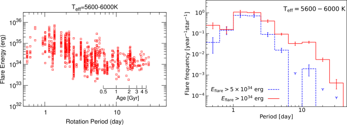
Left: Scatter plots of flare energy versus rotation period of superflares (reproduced from Okamoto et al. 2021). They differ based on stellar temperature values: \(T_{\mathrm{eff}}=5600\text{--}6000\text{ K}\). Scale of stellar age is added based on gyrochronology relation (age versus rotation period relationship) for solar-type stars (Ayres 1997). Right: Relationship between frequencies of superflares with energies greater than \(10^{34}\text{ erg}\) and \(5\times 10^{34}\text{ erg}\) and a rotation period of star (from Okamoto et al. 2021)
Fig. 12 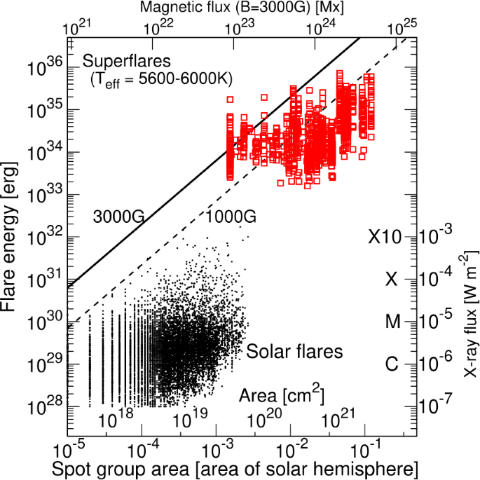
Area of starspots on the horizontal axis and flare energy on the vertical axis for both solar flare data and superflare data found in Kepler Space Telescope data (from Okamoto et al. 2021). The vertical axis on the right shows GOES flux intensity, which corresponds to flare energy. Note that the correlation points for the solar events (lower left) contain an artefact: in the original source of these points (Sammis et al. 2000) no allowance was made for loss of sensitivity for the weaker events (Wheatland 2000; Hudson 2021). This explains the lack of points at the lower right and greatly changes the nature of the perceived correlation, if any
-
(iii)
The frequency of superflares on young, rapidly rotating stars (\(P_{ \mathrm{rot}}=1-3\) days) is ∼100 times higher compared with old, slowly rotating stars (\(P_{\mathrm{rot}}>20\) days), and this suggests that as a star evolves (and its rotational period increases), the frequency of superflares decreases (Fig. 11).
-
(iv)
The flare occurrence frequency distributions of each \(P_{\mathrm{rot}}\) show nearly power-law distributions (Fig. 13). The occurrence distributions of superflares on Sun-like stars and of solar flares are roughly on the same power-law line (Figs. 9 & 13). From the analysis of Sun-like stars, superflares with energy \({\sim }7\times 10^{33}\text{ erg}\) (∼X700-class flares) and \({\sim }10^{34}\text{ erg}\) (∼X1000-class flares) can occur once every ∼3000 and ∼6000 yr, respectively, on the Sun (Fig. 9).
Fig. 13 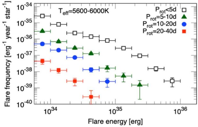
Occurrence frequency distributions of superflares on solar-type stars with temperatures between 5600 and 6000 K (from Okamoto et al. 2021). Data are divided by rotation period
-
(v)
The solar-type superflare stars found by Okamoto et al. (2021) have no confirmed exoplanets, and this indicates that a hot Jupiter is not a necessary condition for superflares on solar-type stars.


As for a more comprehensive review of the statistical studies of superflares on solar-type stars described in Sects. 3.1–3.3, see also the recent book chapter by Hayakawa et al. (2023c).
The possibility of superflares with energy \(>10^{34}\text{ erg}\) to occur on our Sun has been under debate. Aulanier et al. (2013) suggested that it is unlikely that the current solar convective dynamo can produce giant sunspot groups necessary for such large superflares, since such groups have not been observed over the last few hundred years (see Schrijver et al. 2012). The above results of Okamoto et al. (2021), however, showed that slowly rotating Sun-like stars (\(T_{\mathrm{eff}}=5600\text{--}6000\text{ K}\), \(P_{\mathrm{rot}}=20\text{--}40\) days, and age \(t\sim 4.6\) Gyr) can have starspots with a size of ∼1% (10,000 msh) of the solar hemisphere (see also Maehara et al. 2017; Notsu et al. 2019). This can be enough to produce \(10^{34}\text{ erg}\) superflare (cf. Fig. 12), and the upper limit of the superflare energy of these Sun-like stars in this study (e.g., Figs. 11 and 13) is roughly in the same range. Shibata et al. (2013) also suggested that even the current Sun can generate large magnetic flux necessary for \(10^{34}\text{ erg}\) superflares in a typical dynamo model. These results support the possibility of superflares occurring on the Sun and reveal the frequency of superflares on the Sun through the Sun-like stars.
3.4 Further Investigations of Superflares on Sun-Like Stars
Despite the large progress outlined above, the current estimates of the flare occurrence in solar-like stars and their implications for the Sun are still far from being final. In this subsection, we outline two important directions which require further investigations.
3.4.1 The Choice of the Stellar Sample
The main idea behind the use of stellar data to estimate possible ranges of solar variability (driven by both eruptive events like flares or other mechanisms like stellar rotation and activity cycles, see e.g., Kopp and Shapiro 2021) is to compensate a relatively short period of direct solar and stellar observations by a large number of comparison stars. Strictly speaking, this idea would only work if the stars chosen for comparison are true analogues of the Sun. In other words, the underlying assumption of making solar projections based on stellar data is that if each individual star in the stellar sample and the Sun were observed long enough they would yield identical ranges of variability and flare occurrence. Thus, the choice of the stellar sample is one of the most critical issues for making solar projections, and there are several examples in the literature when the improper choice of the stellar sample plagues the resulting solar projection. Wright (2004) found that “To date, there is no unambiguous identification of another star in a Maunder minimum state.”
The studies listed in Sects. 3.1–3.3 have been focused on the so-called solar-like stars, i.e. stars with near-solar effective temperatures and rotation periods. These two parameters are believed to define the action of stellar magnetic dynamo (e.g., Skumanich 1972; Noyes et al. 1984; Reiners 2012) which drives all manifestations of stellar activity, including flares. While stellar effective temperature can be determined for Kepler stars from colour photometry (see, e.g. Berger et al. 2020), the rotation periods for most of the G-dwarfs in the Kepler field are currently unknown. For example, the survey of McQuillan et al. (2014) used by Notsu et al. (2019) and Okamoto et al. (2021) contains rotation periods for only 16% of Kepler stars with near-solar effective temperatures (5500–6000 K). The reason for this scarcity of rotation periods is that the majority of Kepler stars display highly irregular light curves. The irregularities have been connected to short starspot lifetimes and the interplay between contributions of dark spots and bright faculae to the photometric variability (Shapiro et al. 2020; Reinhold et al. 2021). In particular, it was shown that if the Sun was observed by Kepler, its rotation period could not be reliably determined using standard techniques (Amazo-Gómez et al. 2020), e.g. the auto-correlation analysis as performed by McQuillan et al. (2014). Consequently, the estimates based on the analysis of stars with known rotation periods potentially do not include (or rather exclude) most of the stars truly similar to the Sun. This might bias the solar-stellar comparison studies (see detailed discussion in Reinhold et al. 2020). Possible ways to assess the importance of this bias and at least partly remove it include uncovering rotation periods of more stars like the Sun (see, e.g. recent effort by Santos et al. 2021; Reinhold et al. 2022) or utilize proxies of stellar magnetic activity which do not depend on the rotation period (e.g. measurements of stellar Ca II H&K emission, see Karoff et al. 2016).
3.4.2 Contamination of Stellar Light Curves
The focal plane of the Kepler telescope consists of 42 charge-coupled devices (CCDs) with almost a hundred million pixels. The photon flux from each target star is distributed over several pixels, and to extract it, different aperture masks are used (see squares with white borders in Fig. 14). The pixels included in these masks are often affected by background stars so that the Kepler light curves yielded by different pipelines (see, e.g. Stumpe et al. 2014) might be polluted by signals not associated with the target stars. In particular, some of the flares in stellar light curves might occur not on the target but on background stars. Such pollution could be safely neglected in studies of active stars which show frequent superflares. However, the superflares on solar-like stars used in solar-stellar comparison studies are extremely rare so that even small pollution by more active background stars (with more frequent superflares) might significantly affect the estimate of flare occurrence on solar-like stars and, consequently, on the Sun.

Examples of the Kepler light curves with flare candidates (left columns) and localisation of the signal in Kepler CCDs for the two subsequent cadences of the flare candidates (middle and right columns). The star symbols are colour-coded according to their apparent Gaia magnitude Gmag. The blue dots represent 1000 realizations of the flare position obtained from the Markov chain Monte Carlo (MCMC) fitting, and the red ellipses show the 68%, 95%, and 99.9% confidence regions. Squares with white borders show the pixels of the aperture mask used to extract the light curve. Top row: example of the true flare associated with the target star. Middle row: example of flare occurring on background star. Bottom row: a transit of a Solar-system object across the image. The panels are adapted from Vasilyev et al. (2022)
Recently, Vasilyev et al. (2022) developed a Bayesian approach that fits the Kepler point spread function to determine the most likely location of the flux excess associated with flare candidates on CCD. This approach allowed them to check whether the flux excess comes from the target star and, thus, either confirm or reject the flare candidate. They analyzed 5862 solar-like stars and found 2274 events with flux exceeding a 5\(\sigma \) threshold above the running mean for at least two consecutive data points (separated by 30 minutes) in the light curve. Interestingly, Vasilyev et al. (2022) found that only 283 events (i.e. about 12% of the total amount) are associated with target stars (Fig. 14, top row). Most of the events are not associated with any star from the Gaia DR2 catalogue (Gaia Collaboration et al. 2018), while 47 events are associated with background stars listed in Gaia DR2 (Fig. 14, middle row). Finally, several events are associated with transits of Solar System objects (Fig. 14, bottom row). This led Vasilyev et al. (2022) to the conclusion that analysis of the light curve alone is insufficient for identifying stellar flares and future studies must also analyze the instrument pixel-level to carefully exclude contamination of the light curves.
It is noted that to avoid false detection of flares on neighbouring background stars, previous studies selected isolated stars (e.g., Shibayama et al. 2013); Okamoto et al. 2021. This criterion, however, often removes more than half of the stars from the initial target list (e.g., Shibayama et al. 2013, removed 70% from the initial sample). The method introduced by Vasilyev et al. (2022) does not require any sample reduction and allows us to detect flares on stars originally excluded in previous studies. That might help to improve statistics and provide a better estimate of the superflare occurrence frequency on Sun-like stars, and further future studies are important.
3.5 Recent Attempts to Detect Stellar Coronal Mass Ejections
3.5.1 How to Detect Stellar CME?
Solar flares are sometimes accompanied by mass ejections such as filament and prominence eruptions (PEs/FEs) and CMEs. Are superflares accompanied by super-CMEs? This is an important question not only for studying extreme solar events but also for studying exoplanets’ atmosphere and habitability. However, direct observations of stellar CMEs are not easy since we cannot obtain spatially resolved images of distant stars.
There are several approaches how to search for stellar mass ejections. The first one is to detect blue-shifted emissions from the erupted plasma. In the case of M-type flare stars, enhancements in the blue wing of chromospheric lines (blue-asymmetries) are sometimes observed during flares (see Fig. 15 or e.g., Honda et al. 2018; Vida et al. 2019; Maehara et al. 2021). The line-of-sight velocity of these blue-shifted components ranges from a few tens to 600 km/s (e.g., Vida et al. 2019), which is roughly comparable to the average velocity of solar prominence eruptions (e.g., Gopalswamy et al. 2003). Moreover, blue-shifted coronal emissions have been reported in the RS CVn-type binary with high-resolution X-ray spectroscopy (e.g, Argiroffi et al. 2019). These blue-shifted emissions are thought to be caused by the upward flow of chromospheric/coronal plasma due to prominence eruptions and coronal mass ejections.

Top: Light curves of the flare on the M-dwarf YZ CMi. Black-filled circles with solid lines indicate temporal variations of the stellar brightness in the optical continuum (observed with TESS). Red circles with dashed lines indicate temporal variations of the H\(\alpha \) equivalent width. Middle: Temporal variation of the preflare-subtracted H\(\alpha \) line profile during the flare. Bottom: Preflare-subtracted H\(\alpha \) line profile at \(t=52\text{ min}\) (first peak of the H\(\alpha \) light curve). Black-solid line and red-dashed line represent the observed and model line profiles. The observed H\(\alpha \) line profile can be modelled with a two-component Gaussian model with \(v=0\text{ km}/\text{s}\) (blue-dotted line) and \(v=-86\text{ km}/\text{s}\) (blue-dash-dotted line). Data from Maehara et al. (2021)
The second approach is to detect X-ray absorptions associated with flares. X-ray observations of active stars found that sudden increases in absorbing column density are sometimes observed during flares (e.g., Haisch et al. 1983; Favata and Schmitt 1999). The potential cause of these events is the passage of cool and dense plasma (e.g., prominence) across the line of sight. Therefore, the transient increases in absorbing column density associated with flares are thought to be the possible signature of stellar PEs/FEs and CMEs (e.g., Moschou et al. 2017).
The third approach is to detect the coronal dimming in EUV and X-ray wavelength. In the case of the Sun, EUV or X-ray dimming events are sometimes associated with CMEs (e.g., Sterling and Hudson 1997; Thompson et al. 2000). These dimmings are thought to be caused by the coronal density decrease due to the loss or expansion of coronal materials (e.g., Zarro et al. 1999). In the case of stellar flares, Veronig et al. (2021) found several post-flare X-ray dimming events on the M-type star Proxima Cen and K-type star AB Dor. In addition, post-flare UV dimmings on the M-type flare star EV Lac and K-type star \(\epsilon \) Eridani were reported by Ambruster et al. (1986) and Loyd et al. (2022). By analogy with the solar cases, these stellar X-ray and UV dimming events are thought to be possible evidence of stellar CMEs.
The last approach is to detect stellar type II and type IV radio bursts. Type II solar radio bursts are nonthermal radio emissions with a frequency below \({\sim }200\text{ MHz}\) showing negative frequency drifts. They are explained by plasma emissions near the electron plasma frequency (and its harmonics) generated by CME-shock accelerated electrons. Therefore, stellar type II bursts are thought to be strong evidence of stellar CMEs. However, no successful detection of type II bursts from stars other than the Sun has been reported yet (e.g., Crosley and Osten 2018a,b). The reasons for the non-detection of type II bursts are still under debate (e.g., Mullan and Paudel 2019; Alvarado-Gómez et al. 2018, 2020). In the case of the Sun, CMEs are sometimes accompanied by broadband radio emissions called Type IV radio bursts (e.g., Gopalswamy 2011; Bain et al. 2014). These radio emissions are thought to be generated by synchrotron or gyro-synchrotron emission of electrons trapped within CME flux ropes. Zic et al. (2020) reported a stellar type IV burst from the dMe star after an optical flare. Although type IV bursts are thought to originate from several different physical processes (e.g., Morosan et al. 2019) and may not be conclusive evidence of CMEs, some stellar type IV bursts can be possible signatures of stellar CMEs.
3.5.2 Stellar Filament Eruption Associated with a Superflare on Young Solar-Type Star
In the case of the Sun, filament eruptions on the solar disk can be observed as the blue-shifted absorption features in the H\(\alpha \) image of the Sun (e.g., Shibata et al. 2011). Figure 16 shows the temporal variation of Sun-as-a-star H\(\alpha \) spectra during a solar flare and a subsequent filament eruption (Otsu et al. 2022, for more investigations on Sun-as-a-star H\(\alpha \) spectra, see also). The flare can be seen as an emission at the line centre, and the filament eruption can be observed as a post-flare dimming caused by a blue-shifted absorption. This suggests that transient blue-shifted absorption components in the H\(\alpha \) line could be strong evidence for filament eruptions from solar-type stars.

Top: H\(\alpha \) images of the C-class flare and subsequent filament eruption that occurred on 2 April 2017 obtained with the SMART/SDDI (Ichimoto et al. 2017). Middle: X-ray and H\(\alpha \) light curves of this event. Black-solid line and red-dashed line with open circles represent the GOES X-ray (1–8 Å) flux and temporal variations of the Sun-as-a-star H\(\alpha \) line equivalent width. The H\(\alpha \) line equivalent width shows the post-flare dimming. Bottom: Temporal variation of H\(\alpha \) line (dynamic spectrum) during this event. The dynamic spectrum suggests that the early phase of post-flare dimming in the H\(\alpha \) light curve is caused by the blue-shifted absorption component due to the filament eruption. Data from Namekata et al. (2022)
Namekata et al. (2022) reported the detection of a giant filament eruption associated with a superflare (\(E_{\mathrm{flare}} \sim 2\times 10^{33}\) erg) on the young solar-type star EK Draconis. Figure 17 shows light curves and dynamic spectra of the H\(\alpha \) line during the superflare, respectively. As shown in the dynamic spectrum of the H\(\alpha \) line, although the flare can be seen as an emission at the line centre, the post-flare dimming observed in the H\(\alpha \) light curve was caused by the blue-shifted absorption component with a velocity of \({\sim }500\text{ km}/\text{s}\). This velocity is \({\sim }6\) times larger than the average velocity of solar prominence eruptions (\({\sim }80\text{ km}/\text{s}\), Gopalswamy et al. 2003). Furthermore, during the post-flare dimming, the blue-shift velocity of the absorption component decreased with a deceleration rate comparable to the star’s surface gravity. These observational features are similar to the post-flare dimming and blue-shifted absorption due to the filament eruption in the Sun-as-a-star H\(\alpha \) spectra. If we assume that the filament eruption on the star causes the blue-shifted absorption in the H\(\alpha \) line, the mass of erupted material is estimated to be \(10^{18}\text{ g}\), which is \({\sim }10\) times larger than that of the most massive solar CMEs. These results suggest that superflares on solar-type stars can produce fast and massive filament eruptions.

Top: TESS (optical continuum) and H\(\alpha \) light curves of the superflare on EK Dra. Bottom: Dynamic spectra during this event. Data from Namekata et al. (2022)
3.5.3 Future Prospects
Although several observational signatures for the stellar mass ejections have been reported, it is still under debate whether stellar flares can produce stellar CMEs. This is mainly because the typical velocity of mass ejection candidates is smaller than the escape velocity of the stars (e.g., Vida et al. 2019). In addition, several numerical studies (e.g., Drake et al. 2016; Alvarado-Gómez et al. 2018) suggested that CMEs from the magnetically active stars would be suppressed by the strong overlaying magnetic fields by analogy with the non-CME-productive active region on the Sun (e.g., Thalmann et al. 2015; Sun et al. 2015). Figure 18 shows the ejected mass and kinetic energy as a function of flare energy. According to Takahashi et al. (2016) and Kotani et al. (2023), the mass of CME/filament (\(M\)) can be expressed by
where \(\rho \), \(H\), and \(L\) are the density, the pressure scale height, and the length scale of the active region, respectively. On the other hand, the total energy released during the flare can be estimated by the magnetic energy stored in the active region with the length scale of \(L\). Using the fraction of the energy released by the flare \(f\), the total flare energy can be written as
where \(B\) is the magnetic field strength. Therefore, equations (1) and (2) lead to the following scaling relation (cyan-dashed line in Fig. 18a):
Estimated masses of erupted materials for stellar events are comparable to the expectation from the scaling relation for solar CMEs. However, kinetic energies of ejected materials for stellar cases estimated from the blue-shift components in the H\(\alpha \) line are one–two orders of magnitude smaller than expected from the empirical relation for solar CMEs (e.g., Moschou et al. 2019; Maehara et al. 2021; Namekata et al. 2022). The velocity difference between prominence/filament eruptions and CMEs (e.g., Gopalswamy et al. 2003) or the velocity suppression due to the strong overlying magnetic fields (e.g., Alvarado-Gómez et al. 2018) have been proposed as possible interpretations of this discrepancy (e.g., Namekata et al. 2022).

(a) The estimated mass of solar CMEs, prominence eruptions, and candidates of stellar mass ejections as a function of flare energy (data from Yashiro and Gopalswamy 2009; Drake et al. 2013; Moschou et al. 2019; Maehara et al. 2021; Namekata et al. 2022). The cyan-dashed line indicates the scaling relation between the CME mass and flare energy (e.g., Takahashi et al. 2016; Kotani et al. 2023). (b) Same as (a) but for the kinetic energy. The cyan-dashed line indicates \(E_{\mathrm{kin}} = E_{\mathrm{flare}}\) (e.g., Emslie et al. 2012)
In order to unveil the connection between stellar flares and stellar CMEs, we need to obtain signatures of stellar mass ejections with different methods from the same event. Therefore, simultaneous and multi-wavelength observations of stellar flares are important. For example, X-ray/EUV observations simultaneously with optical photometry and spectroscopy allow us to investigate whether the X-ray and EUV dimmings due to CMEs are associated with the H\(\alpha \) blue-shited events caused by prominence/filament eruptions. Furthermore, radio observations to search for stellar type II bursts with low-frequency radio telescopes, such as LOFAR and SKA, are also important since they are thought to be the most promising evidence for stellar CMEs. Simultaneous radio, optical, and X-ray observations enable us to clarify whether stellar prominence/filament eruptions observed as blue-shift events can lead to stellar CMEs.
4 Extreme Solar Events from Cosmogenic Data
4.1 Introduction
The energy of SEPs is usually lower than that of GCRs but can still reach several hundred MeV or even several GeV during the GLE events (see Sect. 2.2.1), which is sufficient to cause the nucleonic cascade and produce cosmogenic nuclides in the atmosphere. Representative cosmogenic nuclides with relatively long half-lives include carbon-14 or ‘radiocarbon’ (14C, half-life ≈5730 years), beryllium-10 (10Be, half-life \({\approx} 1.4 \times 10^{6}\) years), and chlorine-36 (36Cl, \({\approx} 3 \times 10^{5}\) years). They are preserved in natural archives such as tree trunks (by uptake of 14C from the air) and ice sheets (10Be and 36Cl through sedimentary processes, i.e., gaseous, wet and dry depositions – see details in Sect. 6). The production of cosmogenic nuclides in the atmosphere depends on the energy spectrum of energetic particles impinging on Earth, e.g., SEPs (Webber et al. 2007; Mekhaldi et al. 2015, 2021; Poluianov et al. 2016).
Among all GLE events, the strongest hard-spectrum (GLE#5 on 23-Feb-1956) and soft (GLE#24 on 04-Aug-1972) are considered to have produced the greatest amount of 14C (and 10Be) and 36Cl, respectively, during the last decades (e.g., Usoskin and Kovaltsov 2012, 2021; Mekhaldi et al. 2021). However, even though these events were the strongest directly observed (e.g., the event-integrated intensity of GLE#5 was about 5200%⋅h above the GCR background as recorded by polar sea-level NMs – Asvestari et al. 2017b), they were still too weak to produce a detectable amount of cosmogenic isotopes (Fig. 19, see also Usoskin et al. 2020; Mekhaldi et al. 2021). This is because the time resolution of cosmogenic-isotope measurements is typically annual at best. Accordingly, the SEP-production signal should be greater than the GCR-related production of the isotope on the annual time scale.

Modelled annually averaged 14C production by GCR and SEPs for the period 1945–1965, without anthropogenic nuclear tests. Panel (a) displays the modelled production rate \(Q_{\mathrm{14C}}\). The solid blue and dashed red curves represent the GCR and reference GLE#5 scenarios, respectively. The GLE#5 curve is offset by 2 (at \(\text{cm}^{-2}\text{ s}^{-1}\)) for better visibility. Panel (b) depicts the modelled \(\Delta ^{14}\)C for the same period. The solid blue, dashed red and dotted green curves correspond to GCR, GCR+10xGLE#5, and GCR+20xGLE#5 scenarios, respectively. Error bars in panel (b) correspond to the best modern measurement uncertainty, 1.5‰, of \(\Delta ^{14}\)C (Güttler et al. 2015; Park et al. 2017). The plot is modified after Usoskin et al. (2020)
An important discovery was made in 2012 when a significant increase in \(\Delta ^{14}\)C in tree rings dated back to 775 CE was reported by Miyake et al. (2012). Later, the event was confirmed in other trees (e.g., Usoskin et al. 2013) and significant increases were also found, for the same time period, in 10Be and 36Cl concentrations in ice cores from Antarctica and Greenland (Mekhaldi et al. 2015; Sigl et al. 2015; Miyake et al. 2015; Sukhodolov et al. 2017). Different scenarios were initially proposed to explain the discovered significant increases in cosmogenic-isotope data, including a nearby supernova, gamma-ray burst or even a cometary impact on Earth (e.g., Miyake et al. 2012; Pavlov et al. 2013; Liu et al. 2014). However, it was soon shown by Usoskin et al. (2013) that only the SEP scenario can explain all the observed facts, including the effect in different isotopes, hemispheric symmetry and very fast response (for details, see Miyake et al. 2019; Cliver et al. 2022). The SEP event that caused the 775 CE event was estimated to be 25–100 times stronger than the strongest directly observed GLE#5 and found to occur during the late Spring – Summer of 774 CE (Sigl et al. 2015; Sukhodolov et al. 2017; Uusitalo et al. 2018). Accordingly, this ESPE can be denoted as 774 CE or 775 CE depending on whether the year of the ESPE or the effect in CIs is emphasized. An indication was found by Uusitalo et al. (2018) that a small polar enhancement might have existed of the \(\Delta ^{14}\)C signal for that event as potentially related to a very strong production localisation in the polar stratosphere, but this needs further confirmation.
Similar, but slightly smaller cosmogenic-isotope increases were also found as corresponding to ca. 994 CEFootnote 3 and 660 BCE, which are also considered to be caused by extreme SEP events (e.g., Miyake et al. 2013, 2019; Mekhaldi et al. 2015; Park et al. 2017; O’Hare et al. 2019; Sakurai et al. 2020). Later, more events have been discovered in different archives so that the present statistic includes five confirmed events and three candidates (see Sect. 4.2). All these events are considered extremely strong SEP events as discussed below.
Since the time resolution of cosmogenic records is typically annual at its best, ESPEs are often considered as instant production of the isotopes. Their exact duration cannot be resolved so that a single SEP event cannot be distinguished from a short series of consequent bursts, but it can be sometimes defined up to a season (3–4 months) using trees with different growing seasons (e.g., Uusitalo et al. 2018). A recent study by Zhang et al. (2022) suggests that the duration of the events can be longer than one year and not related to the phase of a solar cycle, but the limited time accuracy of the used carbon-cycle box model does not allow to rule out the SEP scenario which still remains the main paradigm for the studied events.
Such extreme SEP events and their parent solar eruptions are expected to have a major impact on our modern technological society. This emphasizes the importance of understanding their occurrence rate and the worst-case scenario. Additionally, the spikes in cosmogenic isotopes, caused by the extreme events, have enabled the dating of historical timbers and volcanic eruptions to the precision of one year (e.g., Oppenheimer et al. 2017; Godwin 2017; Kuitems et al. 2021; Philippsen et al. 2021), as well as the accurate synchronization of floating chronologies in ice cores and tree rings (e.g., Sigl et al. 2015). This chapter is focused on recent research results on the SEP event search using cosmogenic nuclides.
4.2 New Events (Update Since 2019)
4.2.1 Large 14C Increases During the Holocene Discovered to Date: 7176 BCE and 5259 BCE
About a decade after the discovery of the 774 CE event in 2012, Brehm et al. (2022) and Paleari et al. (2022a) reported two strong cosmogenic-isotope increases dated to 7176 BCE and 5259 BCE that were comparable to or even exceed the 774 CE event. Interestingly, while the 14C increase corresponding to the 774 CE events was notable even in the IntCal reference data (Reimer et al. 2020) with the decadal resolution (Usoskin and Kovaltsov 2012), the 14C increases at these two other dates were not significant in the IntCal dataset. The 7176 BCE event was discovered from prominent peaks in the 10Be data with 5–6 years resolution, and the 5259 BCE event was discovered from discrepancies in radiocarbon dating in the surrounding ages (Brehm et al. 2022).
Brehm et al. (2022) confirmed both events using multiple tree samples, from Alpine larch, German oak, and American Bristlecone pine for the 7176 BCE event, and Alpine larch, Irish oak, American Bristlecone pine and Siberian larch for the 5259 BCE event (Fig. 20). Rapid 14C increases were confirmed in 7177/7176 BCE and 5260/5259 BCE in these datasets of three or four tree samples (note that only 14C data of the Bristlecone pine for the 5259 BCE event depicts the increase one year earlier, i.e., in 5261/5260 BCE). This offset may be due to a dendrochronological miscount or inaccurate separation of annual rings, but Panyushkina et al. (2022) have also emphasized the importance of cross-correlating different sequences and correcting for timing differences. For these two events, overall 14C variations are similar to those of the 774 CE event, with the maximum 14C increase reaching 19–20‰ in \(\Delta ^{14}\)C (deviation of 14C concentration from a standard of modern value after corrections of age and isotopic fractionation), which is greater than that of the 774 CE event (≈18‰). However, scales of SEP events for the three events in 774 CE, 7176 BCE, and 5259 BCE are comparable after correcting for the variable geomagnetic shielding, which depends on the geomagnetic field strength (Brehm et al. 2022).

Carbon-14 data for the 7176 BCE and 5259 BCE events (Brehm et al. 2022)
Paleari et al. (2022a) collected new 10Be (annual resolution) and 36Cl (4-year resolution) data from the Northern Greenland Ice core Project (NGRIP) site and 10Be at sub-annual resolution from the recent Eastern Greenland Ice core Project (EGRIP) for the 7176 BCE event. Significant increases in 10Be and 36Cl were observed in these datasets, allowing for synchronization of tree-ring and ice-core chronologies – as a result, the original Greenland Ice core Time Scale GICC05 was shifted 54 years towards the present. Also, increases in the three cosmogenic isotopes (14C, 10Be, and 36Cl) are consistent only with the extreme SEP event origin, while contradicting other possible sources such as gamma-ray events (Miyake et al. 2019; Paleari et al. 2022a). Using these new and previous datasets, i.e., from Greenland Ice core Project (GRIP) and EPICA Dronning Maud Land (EDML) in Antarctica 10Be data with ≈6 and ≈5-year resolution, Paleari et al. (2022a) estimated a 36Cl/10Be enhancement ratio of \(1.59 \pm 0.38\) for the 7176 BCE event, which corresponds to a hard energy spectrum similar to that of 774 CE, 993 CE, and 660 BCE events and similar to the 36Cl/10Be ratio for GLE#5, estimated to be 1.57.
Although a notable 10Be increase around 5259 BCE has not been confirmed in the low-resolution datasets (Brehm et al. 2022), a similarity of the 14C variation between the 5259 BCE event and other extreme events suggests an extreme SEP origin for the 5259 BCE event as well. Therefore, 774 CE, 7176 BCE, and 5259 BCE events encompass the greatest SEP events that occurred during the Holocene.
4.2.2 Smaller Events: 1279 CE, 1052 CE and 5410 BCE
In addition to the three events described above, several smaller-size (yet orders of magnitude stronger than the strongest GLEs of the space era) events have also been reported using a high-precision analysis of 14C in tree rings.
Brehm et al. (2021) analyzed 14C concentrations in tree samples from England and Switzerland with the annual time resolution over the past millennium and reported small \(\Delta ^{14}\)C enhancements in 1052 and 1279 CE. These 14C variations can be explained by short-term 14C production increases in the atmosphere that is consistent with extreme SEP events (Brehm et al. 2021). The scale of these \(\Delta ^{14}\)C enhancements is approximately one-third of that for the 774 CE event. Terrasi et al. (2020) also mentioned a \(\Delta ^{14}\)C enhancement around 1054/1055 CE in Arctic pine and California sequoia trees and suggested, as a possible source, the Crab supernova (SN) explosion in 1054 CE (SN1054). In such a case, \(\gamma \)-rays from the explosion could produce 14C in the atmosphere through photonuclear reactions (e.g., Konstantinov and Kocharov 1965; Damon et al. 1995). However, Kaiser Kudsk et al. (2022) found no significant increase in 1054/1055 CE (i.e., no association with SN1054) by analyzing the available annually-resolved \(\Delta ^{14}\)C datasets reported so far. On the other hand, they reported a remarkable \(\Delta ^{14}\)C increase from 1048 to 1055 CE. Thus, multiple publications have reported an unusual 14C increase around that age, but its origin has not yet been resolved. Panyushkina et al. (2022) suggested that these different excursions may all relate to the same event, which is manifested differently in different records.
For the 1279 CE event, reported by Brehm et al. (2021), Miyahara et al. (2022) analyzed also 14C concentrations in a Japanese Asunaro tree with ultra-high precision by the repeated measurement of the same ages and confirmed a significant \(\Delta ^{14}\)C increase in 1279/1280 CE. Also, they reported significant 14C increases in 1268/1269 and 1261/1262 CE. Since the time around 1280 CE is considered the beginning of the Wolf grand solar minimum (Usoskin et al. 2007), a possible relationship between the occurrence of these SEP event candidates and a transition phase to a grand solar minimum was discussed (Miyahara et al. 2022). These results need to be confirmed by independent measurements in other tree-ring and ice-core series.
Miyake et al. (2021) reported an annual \(\Delta ^{14}\)C increase in 5411/5410 BCE from tree samples of a Californian Bristlecone pine, Finnish Scots pine, and Swiss larch. Although the scale of this event was probably even smaller than that for the 1052 and 1279 CE events (a factor of ≈0.3 the size of the 774 CE event – Brehm et al. 2022), the profile of the \(\Delta ^{14}\)C variation, i.e., a rapid increase followed by a gradual decrease, is also similar to the SEP-driven events such as the 774 CE event (Miyake et al. 2021).
Usoskin and Kovaltsov (2021) emphasized that there is a large gap between the extreme one-per-millennium events like the 774 CE event, on the one hand, and GLEs detected by modern observations, on the other hand. The statistic of intermediate-size events located in the gap is crucially important to understand the nature of ESPEs, whether they are similar to normal SEP events or form a special, presently unknown type of events. However, such events are currently below the detection limit of the cosmogenic-isotope method (Usoskin et al. 2020; Mekhaldi et al. 2021). It will be important to verify high-precision 10Be and 36Cl data from ice cores to confirm their SEP origin in the future. Since 36Cl data are more sensitive to SEPs, even smaller events might be detected as significant increases above background fluctuations (Mekhaldi et al. 2021).
Moreover, there are some specific issues that can affect the detection of intermediate-size cosmogenic-isotope enhancements. For example, there are seasonal 14C variations (within a few permil) in the atmosphere mainly reflecting transport processes caused by the stratosphere-troposphere exchange. However, such an atmospheric transport effect has not been fully considered in connection with the analysis of annual-ring 14C data and are not captured by the standard carbon-cycle box model. Also, the exact season when a tree absorbs atmospheric carbon may vary depending on the region and tree species. Focusing on the worldwide 14C data for the 774 and 993 CE events, \(\Delta ^{14}\)C increases tend to occur earlier in the higher-latitude trees than lower-latitude ones, which may reflect the atmospheric circulation or difference of seasons of fixing carbon (Büntgen et al. 2018; Uusitalo et al. 2018; Miyake et al. 2022). This can also lead to the polar enhancement of the 14C signal, where high-latitude samples tend to yield slightly larger peaks. Additionally, the local/regional meteorological background effects in ice cores for 10Be and 36Cl are often considered without sufficient details, by applying a simplified parameterized approach. It is important to correctly understand and model such possible biasing factors which can affect our interpretation of the cosmogenic-isotope data, in order to reliably identify the intermediate-size events.
4.2.3 Occurrence Rate of Extreme SEP Event
The known ESPEs and candidates detected using 14C data so far have not necessarily been found by successive and consistent surveys, but rather by targeted samplings of interesting periods found in the existing lower-resolution data. It is worth mentioning that only 16.5% of the past 12,400-years tree-ring record has been sampled and measured annually or biennially for 14C concentrations (Brehm et al. 2022) – see Fig. 21. Therefore, to clarify the occurrence rate of ESPEs during the Holocene, we need detailed information from future successive surveys with high-resolution measurements. Based on the number of years covered by the currently available high-precision data (2030 years) and the detected events/candidates (here five events selected, i.e., 774 CE, 993 CE, ∼660 BCE and 7176 BCE events confirmed by both the tree-ring and ice-core data and one of the largest 14C event in 5259 BCE), Brehm et al. (2022) straightforwardly estimated the occurrence frequency to be between about 1/400 and 1/2400 years. However, it should be noted that the periods covered by high-resolution measurements were not randomly taken but had hints of possible high variability.

Extreme SEP events (black and red) and candidates (grey) along with the periods covered by high-resolution (annual or biennial) 14C analyses (shaded). The plot is adopted after Brehm et al. (2022)
On the other hand, recent results from Usoskin et al. (2023) who inter-compared the direct SEP flux measurements for the space era (Raukunen et al. 2022), ESPE events imprinted in terrestrial cosmogenic isotopes, and the SEP flux averaged over the Mega-year timescale in lunar rocks (Poluianov et al. 2018), suggest that the occurrence frequency of the presently known ESPEs and candidates for the Holocene is consistent with the lunar data. It was also shown by Usoskin et al. (2023) that only about half of the Mega-year-averaged SEP flux is produced by ‘regular’ solar activity while the other half is due to rare but extremely strong ESPE events (see Fig. 22).

The ratio between \(F_{60}\) average SEP fluxes \(\langle{F_{60}}\rangle _{\mathcal{F}}/\langle{F_{60}}\rangle _{ \infty}\), where numerator is limited by the maximum observed SEP flux ℱ and denominator is not limited, as a function of ℱ. Shading represents the 68% c.i. The vertical dashed lines, black and blue, with the red horizontal arrows indicate the upper limits of the SEP flux for the space era and Holocene, respectively. Modified after Usoskin et al. (2023)
The above considerations are based on 14C data, which is sensitive to relatively hard-spectrum SEP events, while soft-spectrum extreme events may not be reflected here. Alternatively, ice-core 36Cl data are more sensitive to lower-energy particles and can record also ESPEs with a soft spectrum (Mekhaldi et al. 2021). Although the acquisition of high-precision 36Cl data is more technically challenging than that of 14C, it is expected that new information on ESPEs will be obtained from the 36Cl (and 10Be) continuous measurements in the future.
Available recent data on 10Be, 14C, and 36Cl are summarized in Table 2 for the known ESPE events and candidates. For each event/candidate, the data source and type of the measurement are listed, which can be either the absolute production \(Q_{\mathrm{ESPE}}\) or the peak-factor \(P\) which is the ratio of \(Q_{\mathrm{ESPE}}\) to the GCR background isotope’s production \(Q_{\mathrm{GCR}}\). Two recent archeo/paleomagnetic reconstructions (represented by the virtual axial dipole moment, VADM) for the time of the events are also shown.
5 Modelling: Cosmogenic-Isotope Production and ESPE Spectra Reconstruction
5.1 Mechanism of Production
When cosmic-ray particles enter the Earth’s atmosphere, they interact with air species, specifically, nitrogen, oxygen, and argon atoms. Among various effects and reactions, driven by cosmic rays, e.g., ionisation, fluorescence, radio-emission, incident cosmic particles can interact with nuclei of ambient atoms, leading, in particular, to the production of new nuclides and secondary hadronic particles, mainly protons and neutrons. Those secondaries often carry energy sufficient for their interactions with nuclei to generate new secondaries and nuclides forming the so-called cosmic-ray-induced atmospheric cascade. Here we leave aside rare reactions of nuclide production by pions and kaons, as well as by high-energy photons, and focus on the main nuclide production channel via protons, neutrons, and \(\alpha \)-particles. Secondary nuclides, whose source is the production by cosmic rays, are called ‘cosmogenic isotopes’Footnote 4 (CIs).
After production, cosmogenic isotopes can decay or get involved in chemical processes, being transported with air masses and deposited to the ocean, ice, ground, etc. These processes are important for key isotopes used in the SEP studies and are described in the following Sect. 6, as well as in a comprehensive review by Beer et al. (2012).
Most CIs are produced when energetic particles spall nuclei of target atoms. Those reactions (e.g., 14N(\(x,y\))10Be) require relatively high energies, above ten MeV, of the incident particles. The incident particles denoted here as \(x\) are usually protons, neutrons or primary cosmic-ray ions, and \(y\) are secondary nucleons. There is also another efficient channel of production of some cosmogenic nuclides: the (n,p)-reaction induced by neutrons. In this way, with 14N(n,p)14C possible even for thermal (sub-eV) neutrons, the vast majority of radiocarbon atoms are produced in the atmosphere.
In the light of ESPE studies, the direct production of CI by energetic protons is important, e.g., the reaction 40Ar(p,x)36Cl for 36Cl. That reaction is highly efficient with the maximum cross-section of \({\approx} 100\) mb. In contrast, the maximum cross-section for the production of 10Be from nitrogen and oxygen by protons is 2–4 mb (Beer et al. 2012). Therefore, the overall production of 36Cl is more effective for lower-energy primary protons than the production of 10Be and 14C (see Fig. 25 and the description below, also Koldobskiy et al. 2022). This allows us to use this difference for the reconstruction of spectral properties of ESPEs, as described in more detail in Sect. 5.4.
Most cosmogenic isotopes are unstable and decay, though with different half-life times, ranging from milliseconds to megayears. Different half-life times define the practical applicability of cosmogenic isotopes and also the time scale of cosmic-ray reconstructions possible with them. Three main isotopes used in SEP studies and reconstructions of solar activity over long-term scales are 10Be (half-life 1.39 Myr), 14C (5.73 kyr), and 36Cl (0.30 Myr). As mentioned above, 14C is mainly measured in trees or other organic samples, while 10Be and 36Cl are studied in surface snow and ice cores, taken mostly from ice sheets in Greenland and Antarctica.
5.2 Modelling of Production
The production of cosmogenic isotopes in the Earth’s atmosphere can be quantitatively modelled under different assumptions. A list of recent models of cosmogenic-isotope production is shown in Table 3. Most models are focused on isotopes of beryllium and radiocarbon. This can be explained by their high importance in many different fields of space- and geoscience, as well as in archaeology.
A typical modelling scheme of the CI production rate, using the yield-function approach, is shown in Fig. 23. To model the CI production in a narrow layer of air, the following auxiliary information is needed: (a) composition and density profile for the whole atmosphere; (b) energy/rigidity spectra of primary CR particles (GCR, SEP) bombarding the atmosphere; (c) local geomagnetic shielding represented by the geomagnetic cutoff rigidity \(P_{\mathrm{c}}\) as a function of the latitude and longitude; and (d) cross-sections of the nuclear reactions leading to the production of the isotope.

Schematic representation of the modelling of the cosmogenic-isotope production using the yield-function approach. Green boxes indicate input data which can be measured or independently modelled. The yield function can be calculated separately and thus serves as an input. Yellow boxes correspond to modelling and computation procedures. The pink box “Nuclide production (rate)” is the result of modelling
The CI modelling is usually done for ‘typical’ spectra for GCR or SEP particles. For GCRs, a simple force-field approximation (e.g., Gleeson and Axford 1968; Caballero-Lopez and Moraal 2004; Usoskin et al. 2005) of the spectrum works reasonably well. It is somewhat inaccurate in the low-energy part of the spectrum (\(E<\)100 MeV, Caballero-Lopez and Moraal 2004; Herbst et al. 2017), whose contribution to the CI production is small because such low-energy particles cannot initiate a developed atmospheric cascade. The force-field approximation describes the heliospheric modulation of the local interstellar spectrum (LIS) of GCRs, \(J_{{\mathrm{LIS}},i}(E)\) with units of (cm2 s sr GeV/nuc)−1, in the following way:
where \(J_{i}(E, \phi )\) is the GCR particle spectrum, specifically, the differential intensity of particles of type \(i\) given in (cm2 s sr GeV/nuc)−1, \(E\) is the particle’s kinetic energy per nucleon (in GeV/nuc), \(E_{0}=0.938\text{ GeV}\) is the rest energy of a proton and \(\Phi _{i}=\phi \cdot Z_{i}/A_{i}\). Index \(i\) denotes the specie of cosmic-ray particles, i.e., protons or \(\alpha \)-particles, while \(A_{i}\) and \(Z_{i}\) are their mass and charge numbers, respectively. The \(\alpha \)-particles typically effectively include heavier (\(Z>2\)) ions because they have similar ratios \(Z/A\approx 0.5\). The heliospheric modulation of the GCR intensity is represented by the heliospheric modulation potential (also called ‘modulation parameter’) \(\phi \) (in GV), which is higher during solar active periods and lower when the Sun is quiet. While the modulation parameter formally represents the mean rigidity loss of a particle travelled from the heliospheric boundary to the Earth’s orbit, it has no direct physical interpretation and is just a useful parameterization to describe the GCR spectral modulation. There are different estimates of LIS (e.g., Garcia-Munoz et al. 1975; Burger et al. 2000; Vos and Potgieter 2015; Corti et al. 2016; Herbst et al. 2017), which may differ from each other by up to a factor of two in specific energy ranges (e.g., Asvestari et al. 2017a). Most recent LIS estimates are well-constrained in the low-energy range \({<}500\text{ MeV/nuc}\) by the Voyager in situ measurements in the outer layers of the Heliosphere (e.g., Stone et al. 2013) and in the high-energy range (>50 GeV/nuc) by space-borne astroparticle experiments PAMELA and AMS-02 at 1 AU (Adriani et al. 2013; Aguilar et al. 2021), but remain uncertain in the GeV-energy range which is most important for the CI production. Accordingly, the exact value of \(\phi \) slightly depends on the used representation of LIS and needs to be corrected for that (Usoskin et al. 2005; Herbst et al. 2010). Local interstellar spectra of GCR species heavier than a proton (\(A_{i}/Z_{i}\approx 2\)), mostly 4He nuclei (\(\alpha \)-particles), are often scaled from the proton spectra. These heavier species form 25–30% of the GCR nucleon intensity for the given energy per nucleon (Koldobskiy et al. 2019).
The spectral shape of SEPs can be approximated by various parametric models including the exponential decrease over rigidity, a power law over rigidity or energy, a modified power law, the Band function, Ellison-Ramaty function and many others (e.g., Ellison and Ramaty 1985; Band et al. 1993; Cramp et al. 1997; Miroshnichenko 2015). For SEPs, only energetic protons are usually considered, because the contribution of the less abundant heavier ions in the SEP composition to the CI production is negligible.
Since CIs are produced as a sub-product of the cosmic-ray-induced atmospheric cascade, it is necessary to model the cascade development. Earlier, it was calculated (semi)analytically, using simplified analytical approaches (see, e.g., a review by Gaisser et al. 2016), but currently, with the availability of high computational power, it is standardly done with Monte Carlo modelling and specialized software tools such as, e.g., CORSIKA (Heck et al. 1998), FLUKA (Ferrari et al. 2005), Geant4 (Agostinelli et al. 2003), MCNP(X) (Werner et al. 2017), PHITS (Sato et al. 2013). These are toolboxes, which allow a selection of different ‘physics lists’, i.e., sets of models for physical effects used in computations. Unfortunately, the existing physics models and the particular choice of the used ‘physics list’ may affect the result (e.g., Pavlov et al. 2017), and so far there is no common agreement on which code and set of physics are the best.
Earlier, it was common to perform Monte Carlo modelling for the cascade directly for a prescribed spectrum of GCRs or SEPs (e.g., Masarik and Beer 1999; Kollár et al. 2000; Masarik and Beer 2009) merging the dash-line block in Fig. 23 with the final calculations of the production. However, this straight modelling approach is not flexible and, for different shapes of the GCR or SEP spectra or any other modifications, the computationally-heavy modelling of the cosmic-ray cascade should be repeated anew often taking a significant amount of time and computational resources. To optimise this, the yield-function approach is used where heavy Monte Carlo simulations of the cascade induced by a unit flux of incident particles with fixed energy are completed to calculate the corresponding yield of the CI (the dash-line block in Fig. 23). After that, the CI production can be relatively easily computed as an integral of the product of the yield function and the cosmic-ray (GCR or SEP) spectrum (Equation (9)) for any spectral shape. This method is commonly used in modelling of the CI production (e.g., Webber et al. 2007; Poluianov et al. 2016; Pavlov et al. 2017), as well as for many other applications.
Yield function \(Y_{i}(E,h)\) is defined as the number of atoms of the CI in question (yield) produced in the atmospheric layer of the unit thickness (1 g/cm2) at the given atmospheric depth \(h\) by the unit flux of (cm2 s sr GeV/nuc)−1 of incident particles of type \(i\) with kinetic energy \(E\) (Poluianov et al. 2020). The yield function \(Y_{i}(E,h)\) (atoms sr cm2/g) is directly related to the production function \(S_{i}(E,h)\) (atoms cm2/g), which is the number of CI atoms produced by a single incident particle of type \(i\) with the kinetic energy \(E\) (Webber et al. 2007). For incident particles with the isotropic angular distribution, the functions are directly related as
Yield functions for the main atmospheric CIs relevant for SEP studies are shown in Figs. 24 and 25.


Columnar (integrated over the full atmospheric depth) yield function \(Y_{\mathrm{col}}(E)\) as a function of the energy of incident particles. Panel (A): columnar yield for 10Be, 14C, and 36Cl produced by incident protons and \(\alpha \)-particles. Panel (B): columnar yields (normalized to unity at 10 GeV energy) for 10Be, 14C, and 36Cl produced by incident protons. The pink area indicates the enhanced sensitivity of 36Cl to low-energy protons compared to 10Be and 14C. The yield function data are from Poluianov et al. (2016)
The CI yield over the atmospheric depths is illustrated with \(Y\) of 36Cl for selected energies of incident protons and \(\alpha \)-particles as shown in Fig. 24. Low-energy primary particles (e.g., \(E=0.2\) GeV/nuc) do not initiate a fully developed cascade, thus they produce CI only via direct spallation of atmospheric nuclei, which is observed as a ‘step’ of the yield at shallow depths <30 g/cm2. Higher-energy particles with \(E>1\) GeV/nuc produce a large number of secondary protons and neutrons, accordingly producing more CI atoms per the incident-particle unit flux with the maximum production at the depth of about 100–200 g/cm2 with gradual decrease deeper in the atmosphere.
Yields of different CI may differ by several orders of magnitude in absolute values, but they have roughly similar shapes in the energy domain increasing with the energy of incident particles. Often, a columnar yield function is considered to represent the yield function integrated over the full atmospheric depth from the top to sea level (\(h=1033\text{ g}/\text{cm}^{2}\))
Such columnar yields for 10Be, 14C, and 36Be CIs are shown in Fig. 25. The difference of \(Y_{\mathrm{col}}\) for the considered CIs observed in the low-energy range (panel B) is caused by features of specific nuclear reactions producing the isotopes. This leads to the enhanced sensitivity of the production of 36Cl to lower-energy protons compared to the production of 10Be and 14C.
The production function \(S(E,h)\) (closely related to \(Y(E,h)\), see Equation (5)) can be obtained by a full Monte Carlo modelling of the cosmic-ray cascade as
where \(l\) indicates the type of secondary particles (protons, neutrons, \(\alpha \)-particles), \(E'\) is the energy of these particles (in MeV), \(E\) is the energy of the incident primary particles of type \(i\), \(\eta _{l}(E')\) is the aggregate cross-section (in cm2/g – see Equation (8)). The output of the Monte Carlo simulation is \(F_{i,l}(E,h,E')\), the intensity spectrum of secondaries (in 1/MeV) per primary nucleon at the atmospheric depth \(h\) (in g/cm2). This quantity depends on the angular distribution of the incident primary particles. Typically, models use the isotropic influx of particles, but fixed-angle (e.g., vertical) cases can be also applied for specific studies.
The aggregate cross-section is defined as
where \(\kappa _{j}\) (in 1/g) is the number of target nuclei (nitrogen, oxygen, argon) in the unit mass of air, \(\sigma _{j,i}\) is the total cross-section (in cm2) of the nuclear reactions between the energetic particle of type \(l\) and the target nucleus of type \(j\) that lead to the production of the CI of interest, and summation is over different species (target nuclei) of air denoted with index \(j\). Cross-section data \(\sigma _{j,l}(E')\) represent the probability of a nuclear reaction leading to the production of the CI of interest to occur and can be quantified via experimental or theoretical ways. Experimental data are thought to be more accurate, but there is a shortage of them, especially for neutron-induced reactions. Gaps between the data points are often bridged by parameterisation (e.g., applying the measured proton cross-sections to the neutron ones), extrapolations to higher energies, the use of theoretically-calculated values, or a mixture of all the above. One of the most popular sources hosting a compilation of various experimental cross-section data is the EXFOR database (https://www-nds.iaea.org/exfor/).
Once the yield function is known, it is straightforward to calculate the CI production rate. The differential isotope’s production rate \(q(h)\) (in atoms/(g s)) at depth \(h\) is defined as the sum of integrals of the products of the yield function and the energy spectrum of primary particles of type \(i\):
The integrand of the formula, viz. the product of the yield function and the particles’ spectrum, is called the differential response function. The integration is above the energy \(E_{i}(P_{\mathrm{c}})\), which corresponds to the local geomagnetic rigidity cutoff \(P_{\mathrm{c}}\). The cutoff rigidity is defined by the location and the geomagnetic field (e.g., Cooke et al. 1991), and it is often calculated using the Størmer’s formula (Glaßmeier et al. 2009) for the eccentric-and-tilted-dipole geomagnetic field (Nevalainen et al. 2013):
where \(R\) and \(R_{\oplus}\) are the distance to the dipole centre and the mean Earth’s radius, respectively, \(M\) is the dipole moment (in \(10^{22}\text{ A}\,\text{m}^{2}\)), and \(\lambda _{\mathrm{G}}\) is the geomagnetic latitude of the location of interest. The dipole moment \(M\), which mostly defines the geomagnetic shielding, can be quantified, depending on the quality of magnetic data, as a true dipole moment (DM), a virtual DM (VDM) or a virtual axial DM (VADM) — see more details in Korte and Constable (2005), Panovska et al. (2019). For the last century, the geomagnetic data are standardly provided by the International Geomagnetic Reference Field (IGRF) presented for 5-year epochs as a set of Gaussian coefficients (e.g., Alken et al. 2021).
The integrated atmospheric CI production rate \(Q(h)\) (in atoms/(s cm2)) is an integral of \(q(h)\) from the top of the atmosphere \(h'=0\text{ g}/\text{cm}^{2}\) to the given depth \(h'=h\):
Integration down to sea level \(h =1033\text{ g}/\text{cm}^{2}\) gives the so-called columnar production rate \(Q_{\mathrm{col}}\).
The approach described in this section provides a theoretically computed CI production rate, total \(Q(h)\) or differential \(q(h)\), as a function of the spectrum of energetic particles entering the atmosphere.
5.3 Cosmogenic Isotope Production Rate
Production rates differ significantly for different CIs as caused by the efficiency of production, i.e., threshold energies, concentrations of target atoms, and cross-sections of the corresponding reactions. For example, the globally averaged production by GCR during a period of moderate solar activity (\(\phi =650\text{ MV}\)) and the contemporary geomagnetic field with \(M=7.8\cdot 10^{22}\text{ A}\,\text{m}^{2}\) is 0.029 atoms/(cm2 s) for 10Be, 1.6 atoms/(cm2 s) for 14C, and 0.0025 atoms/(cm2 s) for 36Cl (Poluianov et al. 2016). The effective energies of production/deposition of CIs 10Be, 14C and 36Cl are 2 GeV/nuc, 2.5 GeV/nuc and 1.95 GeV/nuc for GCRs, and 236 MeV, 234 MeV and 60 MeV for SEPs, respectively (Koldobskiy et al. 2022). The significantly lower effective energy of the production of 36Cl is caused by its highly effective production by low-energy protons as discussed above. The difference in the effective energies of the three CI can be used in reconstructions of energy spectra of ESPEs (e.g., Mekhaldi et al. 2015; Koldobskiy et al. 2023).
The CI production by GCR varies in time due to the modulation of the GCR intensity by solar activity. This dependence is illustrated in Fig. 26, which shows the dependence of the globally-average columnar production rate for three CIs as a function of the heliospheric modulation parameter \(\phi \).

Globally-averaged columnar production rates \(Q_{\mathrm{col}}\) of CIs 14C, 10Be, and 36Cl by GCR as a function of the heliospheric modulation parameter \(\phi \). Panel (A): production rates of the three CI for the contemporary geomagnetic field strength (dipole moment \(M=7.8\cdot 10^{22}\text{A}\, \text{m}^{2}\)). Note that 10Be and 36Cl are scaled up by factors 50 and 500, respectively, for the sake of visibility. Panel (B): production rates of 14C for three states of the geomagnetic field corresponding to its variability during the Holocene: weak (\(M=6 \cdot 10^{22}\text{ A}\,\text{m}^{2}\)), modern (\(M=7.8\cdot 10^{22}\text{ A}\,\text{m}^{2}\)) and strong (\(M=12\cdot 10^{22}\text{ A}\,\text{m}^{2}\)). Data are from Poluianov et al. (2016)
The modelled columnar production rate of 10Be by GCR over the Globe is shown in Fig. 27. One can see that due to the low geomagnetic cutoff over the polar regions, the production rate is maximum there, while it is significantly lower in the tropical regions. Presently (and during most of the Earth’s history) the geomagnetic cutoff is maximal in the equatorial regions and vanishes towards the magnetic poles (Gao et al. 2022b). This leads to the corresponding pattern in the CI production rate. However, during rare excursions or reversals of the geomagnetic field, such as the Laschamp event 41 kyr ago (e.g., Panovska et al. 2019), when the geomagnetic dipole field was greatly weakened, and consequently, the geomagnetic cutoff strongly reduced (Gao et al. 2022a), the CI production rate notably increased. The cutoff rigidity can be slightly reduced during strong geomagnetic storms for several hours (e.g., Kudela et al. 2008) but since the effect is small and not exactly synchronised with SEP events, it is usually neglected.

Panel (A): Global map of the columnar production rate \(Q_{\mathrm{col}}\) of 10Be by GCRs. Panel (B): Latitude profile (zonal mean) of the columnar production rate of 10Be shown in panel A. Computations were done with the model by Poluianov et al. (2016) for the modern geomagnetic field (IGRF, epoch 2015) and moderate solar activity (\(\phi =650\) MV)
The dipole moment of the geomagnetic field varies on the timescales of centuries and millennia by a factor of about two between \((6\text{--}12) \cdot 10^{22}\text{ A}\,\text{m}^{2}\) (e.g., Knudsen et al. 2008; Panovska et al. 2018). These changes are directly translated into the production rate (Fig. 26B), and thus should be taken into account in the modelling.
The CI production rate varies greatly over the altitude in the atmosphere (Fig. 24) as defined by the development of the hadronic component of the cosmic-ray-induced cascade. A significant fraction (30–50%) of CI is produced by GCR in the troposphere, and the rest in the stratosphere. For SEPs, the partition is different due to the softer energy spectrum – most of the isotopes are produced in the polar stratosphere (Golubenko et al. 2022; Adolphi et al. 2023).
5.4 Reconstruction of the ESPE Spectrum
Proper modelling of the CI production is a key ingredient for the estimation of the expected SEP integral flux of ESPEs using the measured cosmogenic isotope data from stratified archives (Sect. 4). Consideration of atmospheric transport and deposition processes (Sect. 6) is also crucial here. Typically, reconstructions of the ESPE spectra are based on the use of 14C transport box models of different complexity (e.g., Siegenthaler 1983; Brehm et al. 2021) and models of beryllium transport and deposition (e.g., Heikkilä et al. 2009; Heikkilä and Smith 2012). For chlorine, the transport and deposition are currently considered similar to those for beryllium.
Presently, the energy spectrum of ESPEs cannot be directly reconstructed from CI data, but the parameters of a prescribed shape can be assessed using data from different CIs. The spectral shape of the ESPE flux/fluence is typically assumed similar to those of strong SEP/GLE events registered during the last 70 years that are presently reconstructed quite accurately (Webber et al. 2007; Raukunen et al. 2018; Koldobskiy et al. 2021). However, no direct verification of the GLE response in cosmogenic isotopes is presently possible because even the strongest GLEs cannot produce a sufficient amount of CI atoms to be detected above the GCR background (Usoskin et al. 2020; Mekhaldi et al. 2021).
Reconstructions of the spectral shape of ESPEs are only possible when data from different CIs are available, viz. from 36Cl with its lower effective energy of ≈60 MeV and from 10Be and 14C whose effective energy is ≈235 MeV. First assessments of the ESPE spectra (Miyake et al. 2012, 2013; Usoskin et al. 2013) were quite uncertain. Kovaltsov et al. (2014) proposed that the fluence of SEP particles with energy above 200 MeV, \(F(>200~\mathrm{MeV}) \equiv F_{200}\), is almost directly proportional to the expected production \(Q\) of 14C for all GLE events, irrespective of their spectral shape. This kind of approach is often called as ‘effective energy’ or ‘bow-tie’ method. Interpolating this result to ESPE events, Kovaltsov et al. (2014) estimated that \(F_{200}\) was close to \(8\cdot 10^{9}\text{ cm}^{-2}\) and \(6\cdot 10^{9}\text{ cm}^{-2}\) for the events of 775 CE and 994 CE, respectively.
The first attempt to reconstruct the ESPE spectral shape was made by Mekhaldi et al. (2015) using, for the first time, 36Cl measurements for the ESPEs of 775 CE and 994 CE. Mekhaldi et al. (2015) considered 13 large GLEs, whose spectral fluences were estimated by Webber et al. (2007), and calculated the expected production of 10Be and 36Cl by these events. Then the authors compared thus modelled ratios 36Cl/10Be with the measured ones and concluded that spectral fluences of ESPEs of 775 CE and 994 CE were consistent with those of hard-spectra GLEs (e.g., GLEs #42 of 29-Sep-1989 or GLE #69 of 20-Jan-2005). Next, using the 10Be data and the specific yield function by Webber et al. (2007), they described the ESPEs of 775 CE and 994 CE as GLE #69 scaled up with the factors of 141 and 51, respectively, leading to the estimates of \(F_{30}\) of \((2.82\pm 0.25)\cdot 10^{10}\text{ cm}^{-2}\) for 775 CE and \((1.02\pm 0.21) \cdot 10^{10}\text{ cm}^{-2}\) for 994 CE. The same approach was used by O’Hare et al. (2019) to estimate the spectral shape of the ESPE of 660 BCE. They concluded that the event was similar in both the spectral shape and magnitude to the ESPE of 775 CE.
The methodology used to reconstruct spectral fluences of ESPEs has been significantly updated recently, in particular, by Paleari et al. (2022a) for the ESPE 7176 of BCE: First, updated yield functions for production of CI (Poluianov et al. 2016) were used in this work; Second, revised GLE spectral reconstructions (Raukunen et al. 2018; Koldobskiy et al. 2021) were utilized as the reference spectra; Third, different reconstructions of the GCR background and related uncertainties were considered. In addition, Paleari et al. (2022a) took advantage of using an ensemble of GLE events, for which the modelled ratio 36Cl/10Be was close (within the uncertainties) to the one obtained for the ESPE, instead of scaling a single GLE event. The final reconstructed fluence of the ESPE of 7176 BCE was found to be significantly softer than that from previous reconstructions of ESPE events, leading to much higher (up to an order of magnitude) fluence in the low-energy (\({<}100\text{ MeV}\)) range.
The most recent reconstruction of ESPE spectral fluences was made by Koldobskiy et al. (2023), who used an ensemble of scaled GLEs to represent the energy spectrum of ESPEs and simultaneously fitted the expected signal of all three CIs, 10Be, 14C, and 36Cl. Additionally, the method developed by Koldobskiy et al. (2023) enables one to estimate the absolute production of 14C by an ESPE, reducing the uncertainties related to GCR background reconstruction. Independent reconstructions of VADM (Knudsen et al. 2008; Panovska et al. 2018) were taken into account along with their uncertainties, for the times of the ESPEs. Measurements of all three CIs were simultaneously fitted with scaled fluences of GLEs, and the best-fit solutions and the related uncertainties were obtained. These improved estimates of ESPEs of 994 CE, 775 CE, 660 BCE yield softer ESPE spectrum in comparison to earlier estimates (Mekhaldi et al. 2015; O’Hare et al. 2019), implying an order-of-magnitude higher flux of low-energy (\({<}100\text{ MeV}\)) SEPs. Reconstructions of SEP fluence for ESPE 7176 BCE performed by Paleari et al. (2022a) and Koldobskiy et al. (2023) are in agreement within the uncertainties.
Figure 28 shows the recent reconstructions (Koldobskiy et al. 2023) of the ESPE fluence for four events: 993 CE, 775 CE, 660 BCE and 7176 BCE. For comparison, integral spectra of several ‘typical’ modern GLEs (#5 of 23-Feb-1056, #24 of 04-Aug-1972, #42–45 of Sep–Oct 1989, and #70 of 13-Dec-2006 from Koldobskiy et al. 2021) are also shown along with the time-integrated SEP flux measured by GOES spacecraft during the period of (05–17)-Dec-2006 (Raukunen et al. 2022), which will be discussed further in Sect. 8.

ESPE fluence reconstructions (Koldobskiy et al. 2023) for four ESPE events (994 CE, 775 CE, 660 BCE, 7176 BCE – solid lines with the shaded 68% confidence intervals) in comparison to those for several GLE events (dashed curves) and GOES measurements for the period from (05–17)-Dec-2006 (Raukunen et al. 2022)
6 Modelling: Transport and Deposition of Cosmogenic Isotopes
6.1 Atmospheric Transport and Deposition of Cosmogenic Isotopes
Cosmogenic isotopes are mostly (about half for GCR and \(>90\)% for SEP) produced in the stratosphere. The produced isotopes are then transported by advective or diffusive atmospheric motions and taken by dry and wet deposition processes to reach ice sheets or trees.
The transport pathways from the stratosphere to the lower troposphere are illustrated in Fig. 29, which shows that a proper simulation of the isotopes’ transport requires adequate representation of the advective circulation as well as diffusive transport. This complex problem can be solved only by 3D general circulation models with reasonable horizontal/vertical resolutions and an adequate representation of different atmospheric waves. The peculiarities of the transport depend on the isotope type. For example, the transport pathway of 36Cl can be different from this scheme because it participates in chemical cycles and can be converted into active (e.g., ClO) and passive (HCl or ClONO2) chemical species. In this case, the advective transport stays intact, but horizontal mixing may be different depending on the vertical and horizontal gradients. Some problems could be also related to distinguishing the production signal from 36Cl transported from the ocean where it is stored in the form of sea salt (NaCl, e.g., Pivot et al. 2019). However, it is more important for the detection of long-term trends and variability, while for ESPEs, the expected spike-like features should be observable rather well. The same is true for the 14C case when the simulation of long-term variability involves interaction with land and oceanic biosphere.

Illustration of the stratosphere-to-troposphere transport pathways (from Holton et al. 1995; Liang et al. 2009, by CC BY 3.0). Eddy transport throughout the tropopause is shown by the wavy arrows. Blue arrows represent slow motion across polar tropopause. The orange and blue arrows demonstrate tropospheric transport. The values in per cent denote the stratospheric contribution over the middle (red) and high (blue) latitudes and characteristic time scales
In the case of 10Be, the complications are related to its attachment to the stratospheric aerosol particles. Under volcanically quiescent conditions, sulfate aerosol particle radius is usually less than 0.2 μm (Pierce et al. 2010) with gravitational sedimentation velocity too small to compete with the vertical wind speed (Zhou et al. 2006; Weisenstein et al. 2015). However, after a strong volcanic eruption, the aerosol size distribution is shifted to larger values. For example, the stratospheric aerosols after the Pinatubo eruption in 1991 had mean radii of 0.4–0.6 μm (Sukhodolov et al. 2018) in the tropical and mid-latitude lower stratosphere, resulting in sedimentation velocities that are comparable to the advective upward motions speed in the tropical meridional circulation branch (Weisenstein et al. 2015), which prevents aerosol (with embedded isotopes) from being transported to the middle stratosphere. Over the mid-latitudes, the annual mean downward wind speed is around 10 km/year (e.g., Zhou et al. 2006), but can reach higher values during dynamically active winter seasons. In this case, the downward advective transport of the volcanic aerosol across the tropopause can be substantially enhanced, reducing the lifetime of stratospheric aerosols. The treatment of this process requires a detailed representation of the aerosol microphysics, which allows one to calculate sedimentation velocities for background conditions as well as for volcanic cases.
An important part of the isotope transport is related to the representation of dry and wet deposition. For these processes, an understanding of the reactivity and solubility of the isotopes is crucial. These quantities are well known for 14CO2, which quickly forms after the 14C production. More complicated isotopes for the modelling are 36Cl and 10Be. Solubility and reactivity of 36Cl depend on the type of the host molecule, and a proper simulation of this process involves complicated changes in the chemical routine. For 10Be, it is important to know whether it is in gas form, with extremely low solubility and reactivity, or attached to sulfate (or another) aerosol particles with different chemical properties. The process implementation requires complicated aerosol microphysics in both the stratosphere and troposphere. Moreover, the SEP production of isotopes is mostly confined to the high latitudes, where significant seasonal and inter-annual variability in the stratosphere-troposphere exchange and the height of the tropopause occur (e.g., Stohl et al. 2003). This introduces an additional uncertainty for the interpretation of observations as well as for modelling since the dynamical conditions of the polar regions can strongly modulate the atmospheric lifetime of the produced isotopes due to the changes in transport pathways and the type of aerosols these isotopes can be attached to.
At the moment, there are no models which are capable of precisely describing all the above-mentioned processes, but the community efforts presented below allow us to hope that most problems will be solved in the near future.
6.2 State of the Art
Among all cosmogenic isotopes, modelling of 10Be and 7Be has been best covered in the past because of their chemical inertness and the possibility to neglect post-depositional processes. Nevertheless, a reliable model for 10Be and 7Be budget calculations would still require a well-resolved stratosphere, to fully cover the production region and stratospheric circulation, as well as a good description of the relevant depositional processes in the troposphere, determined by the local meteorology. Models of such complexity became available already in the early 2000s and since then there has been a lot of progress to simulate the atmospheric budget of beryllium isotopes. Earlier studies characterized, in reasonable detail, the cosmogenic beryllium production, transport, and deposition under various climatic (Field et al. 2006; Heikkilä et al. 2013), geomagnetic (Heikkilä et al. 2009) and solar (Heikkilä et al. 2008) conditions, as well as exploring specific modelling nuances (Heikkilä and Smith 2012; Delaygue et al. 2015). In particular, it was shown that some modern models can accurately reproduce the observed cosmogenic-beryllium production and transport at timescales longer than synoptic (Usoskin et al. 2009; Golubenko et al. 2021). However, they did not address the conditions of extreme solar events because reliable evidence and magnitude estimates for such events became available only with the discovery of the 774 CE event. The first attempt to simulate this event in sufficient detail was performed by Sukhodolov et al. (2017) with the chemistry-climate model SOCOLv3. Besides showing the details of atmospheric impacts of the event, that study also conducted simulations of 10Be and showed a good agreement of simulated 10Be deposition fluxes with the ice core observations in Greenland and Antarctica (Fig. 30A), which confirmed both the magnitude range of the event and the understanding of the global atmospheric processes that govern 10Be pathways from their production regions to the polar ice sheets. However, SOCOLv3 at that time had a simplified treatment of wet and dry deposition in the troposphere and no calculation of beryllium attachment to aerosols. Although such a configuration was still sufficient to match the observations on the annual timescales, it greatly complicated an estimate of the season in which the event could have occurred.

Comparison of modelled and measured concentrations of beryllium isotopes for different time scales and conditions. Panel (A): Annual depositional fluxes of 10Be at two sites analyzed for the period around 774 CE over the WDC (Antarctica) and NEEM (Greenland) stations. Red lines with error bars depict the measured data, while blue lines depict the modelled 10Be flux. Years are given relative to the peak year (775 CE). Plot is modified after Sukhodolov et al. (2017) Panel (B): modelled and measured 7Be concentrations in the near-ground air at the locations of four measurement stations in Canada and Chile. The measured and modelled data are shown as solid red and dashed blue curves, respectively. The plot is modified after Golubenko et al. (2021)
The proton spectra and fluence estimates, used in Sukhodolov et al. (2017), have been later revised both for the GLE#5 (23-Feb-1956) event (Usoskin et al. 2020), whose spectrum was initially used for upscaling the fluence for 774 CE, and the 774 CE event itself. SOCOLv3 was further used by Usoskin et al. (2020) to calculate the expected beryllium signal for the GLE#5 and to estimate the detection limits of ESPEs on the background introduced by solar-cycle variations of GCRs. It was shown that a SEP event by a factor 4–5 stronger than the GLE#5 can be potentially detected in a multi-proxy record.
The SOCOL model was upgraded by Feinberg et al. (2019), by adding detailed descriptions of sulfate aerosol microphysics and interactive wet and dry deposition schemes. The updated version of the model, SOCOL-AERv2-BE, was used by Golubenko et al. (2021) to simulate concentrations of 7Be in near-ground using a full nudging to the meteorological fields for the period of 2002–2008. The modelled concentrations were compared with the measurements at a weekly time resolution in several high-latitude stations of both hemispheres and showed a very good agreement (Fig. 30B). The model correctly reproduced the temporal variability of 7Be concentrations on annual and sub-annual time scales, including the presence and absence of the annual cycle in the Northern and Southern hemispheres, respectively. Similar studies were performed with the GEOS-Chem model (Brattich et al. 2021) to simulate and verify the transport details and surface concentrations of 7Be, which also resulted in a good agreement with the near-surface observations. Although these latter studies were not focusing on extreme events, they presented evidence that state-of-the-art 3D models are able to adequately simulate the transport of species from the stratosphere and their deposition at high latitudes (cf. Usoskin et al. 2009). The uncertainties related to the validation of model data against observations are, however, still high due to the assumption that all 7Be is attached to the aerosol particles collected by aerosol traps (Leppänen et al. 2010, and references therein), while the amount of 7Be in the gas-phase part or in the other aerosol types is actually unknown. Another source of uncertainty is that the typical grid of a global model (1–5∘ in latitude and longitude) sometimes cannot catch the local orography which is important at some locations.
Recently, Spiegl et al. (2022) investigated the transport and deposition of 10Be produced by the ESPE of 774 CE using the 3D Earth-system model ECHAM/MESSy Atmospheric Chemistry (EMAC) model (Jöckel et al. 2016). Contrary to Sukhodolov et al. (2017), that study was focused not on the impact of the 774 CE event on the chemical composition of the atmosphere (e.g., ozone destruction by NOx production), but on the potential influence of the middle atmosphere and troposphere dynamics on the surface-flux signatures of the event. The 10Be production was represented by the GLE#69 (20-Jan-2005) scaled to the magnitude of the 774 CE event (Mekhaldi et al. 2015), using the WASAVIES model (Sato et al. 2018). Transport of 10Be was treated as an aerosol rather than a gaseous tracer, which is of particular relevance for a more realistic scavenging and wet deposition. Figure 31 shows standardized (multi-year mean) monthly anomalies (z-scores) of the zonal mean 10Be mixing ratio for the lower stratosphere and troposphere (at altitudes <30 km, or pressure >10 hPa). It suggests that throughout the northern-hemisphere cold season (October to March), a quasi-hemispheric positive 10Be anomaly slowly descends from the middle to the lower stratosphere, where 10Be atoms accumulate in April after continuous supply from above. A similar pattern was found in the southern stratosphere. During the season of high activity of tropopause folds, positive 10Be anomalies reach the Northern-hemisphere lower subtropical stratosphere, from where they are further distributed towards higher latitudes by the tropospheric circulation between February and May.

Results of the simulation of the transport of 10Be (Spiegl et al. 2022) between the middle stratosphere and the troposphere for different months of a year. Standardized anomalies of the multi-year monthly climatology of the 10Be mixing ratio (colour shaded) from the annual mean for the isotope production taking place in March are shown. Black arrows denote the monthly climatology of the mean meridional circulation (The black arrow at the bottom left corner of each panel row represents a mean meridional velocity of 2 m/s). The dynamical tropopause is shown as the green line. The panels below show the zonal-mean distribution of the tropopause folding frequencies (in %)
In addition, it has been found that the material which is transported downwards from the middle atmosphere to the troposphere is also modulated by an interplay between different tropospheric sink processes, which are characterized by the local meteorology (e.g. the seasonal cycle of precipitation) and determine the seasonal deposition maxima. In this context, generally weaker deposition rates are simulated at probing sites in central Antarctica compared to Greenlandic sites.
6.3 Perspectives
6.3.1 Volcanic Eruptions and Aerosol Properties
Strong volcanic eruptions affect the size distribution of sulfate aerosols in the stratosphere and thus also their transport to the troposphere with subsequent deposition on the Earth’s surface including the polar ice sheets. This also impacts the 10Be transport and deposition, because, after their production in the atmosphere, 10Be atoms get attached to aerosols (Baroni et al. 2011; Raisbeck et al. 1981). Large volcanic aerosols with attached 10Be sediment faster through the lower stratosphere and even across the tropopause, which reduces the stratospheric residence lifetime of 10Be and can ultimately result in a short-term increase of the 10Be concentration in ice cores by up to 112% (Baroni et al. 2019) mimicking an ESPE imprint in ice cores. Sharp and simultaneous increases of 10Be and sulfate concentrations have been observed in ice cores in relation to the eruptions of Agung (1963) and Pinatubo (1991) volcanoes (see Fig. 32 and Baroni et al. 2011). This effect was later confirmed for 14 volcanic eruptions recorded in an ice core from Dome C in Antarctica, covering the last millennium (Baroni et al. 2019). In particular, the 10Be spike ca, 1460 CE, proposed as an ESPE candidate (Usoskin and Kovaltsov 2012), appears to be associated with a major volcanic eruption (Kuwae) rather than with an ESPE. A mechanism involving the microphysics of aerosols was proposed by Baroni et al. (2011) but has never been tested yet with a full 3D chemistry-transport model. Therefore, modelling efforts are necessary to confirm the observationally constrained effect and to better understand the mechanisms of the 10Be transport and deposition in the atmosphere after a volcanic eruption. The applied models should contain detailed aerosol microphysics because aerosol transport dramatically depends on the aerosol size distribution (Seinfeld 2006; Delaygue et al. 2015). Nowadays, models of such complexity became broadly available (Timmreck et al. 2018).

(a) Non-sea-salt sulphate concentration (nss sulphate) in the Vostok ice core (Antarctica). (b) The raw 10Be concentration (blue curve) and that corrected for the volcanic contribution (red curve) for the Agung (Bali, 1963) and Pinatubo (Indonesia, 1991) eruptions using the relationship between the concentrations of 10Be and volcanic sulphate (Baroni et al. 2011). (c) The monthly International sunspot number (V2.0) from SILSO (Clette and Lefèvre 2016)
6.3.2 Modelling of 36Cl
Cosmogenic isotope data is used not only for dating the extreme events but also to estimate their energy spectra (Sect. 5.4). A standard approach for this is based on the use of the 36Cl/10Be ratio (e.g., Mekhaldi et al. 2015; O’Hare et al. 2019). The theoretically expected 36Cl/10Be ratio due to the GCR production is nearly constant at about 0.09 (Poluianov et al. 2016), but for softer particle spectra during ESPEs, the 36Cl production is enhanced with respect 10Be (see Sect. 5.1 for details). Accordingly, an ESPE should result in an increase in the 36Cl/10Be ratio compared with that expected for GCR. This approach has been used to demonstrate that the ESPEs of 774 CE, 993 CE, 660 BCE and 7176 BCE were hard-spectrum SEP events (Mekhaldi et al. 2015; O’Hare et al. 2019; Paleari et al. 2022a; Koldobskiy et al. 2023). It is important that all these estimates were based on the assumption that the 36Cl/10Be production ratio is equal to the 36Cl/10Be post-depositional ratio measured in ice cores, i.e. 36Cl and 10Be are assumed to have identical geochemical cycles, transport in the atmosphere and deposition, as well as post-depositional effects. However, this assumption is not correct and the life cycles of these two cosmogenic isotopes may significantly differ from each other after their production. Moreover, this can additionally be modulated by the climate and atmospheric composition conditions of each particular event. Progress in this direction is possible only with the use of full modelling for the isotopes’ transport and deposition, but a proper model for such an application would have to include both the aerosol microphysics and the gas-phase chlorine chemistry, as well as possible post-depositional effects.
6.3.3 Carbon-Cycle Modelling
As discussed above, possible uncertainties in the complex relations between ESPEs, their signatures in natural archives and atmospheric dynamics in different domains can complicate the interpretation of this new event category and lead to possible uncertainties in geochronological records. In some recent geochronological studies related to the detection of historical ESPEs, such problems have already been expressed. For example, the recently discovered ESPE candidates of 1279 CE (Brehm et al. 2021; Miyahara et al. 2022) and 1052 CE (Terrasi et al. 2020; Brehm et al. 2021) events show comparable small increases in CIs, giving rise to speculations about their possible origin and the possibility of a misinterpretation of their signatures, since they might be significantly masked by local meteorology and climate. Another example of a possible influence of the weather situation on the signatures of cosmogenic isotopes has recently been proposed by Miyake et al. (2022) who report a different temporal timing of the 14C increase during the 993 CE event, obtained from tree rings from different latitudes (i.e., high latitude probes reveal an earlier increase of roughly 1 year compared to the those obtained at lower latitudes). It has been speculated that such kind of regional differences might be caused by an unknown transport process. A similar result was reported by Zhang et al. (2022) who questioned the timing and the duration of some known ESPEs. However, all these studies used a standard 1D box-like model of the carbon cycle (e.g., Büntgen et al. 2018) which is proven to work well for the relatively smooth (spatially and temporarily) production of 14C by GCR but may be inaccurate for the fast and spatially inhomogeneous production by SEPs. Discrepancies like these cannot be resolved by proxy analysis or simple 1D box model approaches alone, thus they need to be complemented by numerical experiments of higher complexity.
Complex Earth-system models with a full-featured interactive carbon cycle are presently already used for long-term climate simulations (Roth and Joos 2013; Arora et al. 2020), but they have not yet been applied for cosmogenic isotope modelling, especially not for relatively short time scales like those of ESPEs. Since complex carbon-cycle models are computationally expensive (e.g. due to the necessary excessive spin-up integration), need a lot of expert knowledge and are typically only available at large atmospheric research facilities, they set up hurdles, especially for the geochronological community. Thus, carbon-cycle models of intermediate complexity, coupled with 3D atmospheric transport models, can become a helpful tool in the context of ESPE studies. In the intermediate-complexity modelling strategies, the uptake of 14C by plants is calculated for a limited number of vegetation types and depends on the atmospheric concentration of CO2, near-surface temperature and precipitation. The carbon fluxes between the ocean and the atmosphere are prescribed based on empirical values throughout the simulation. Such models are currently under development. Even though such intermediate approaches may neglect complex vegetation dynamics (i.e. changes in regional vegetation due to changes in the climate system) or an explicit representation of biochemical processes in the ocean, they capture the essential features of the global carbon cycle quite well as demonstrated e.g. by Obata (2007).
7 Archival Investigations for Historical Space Weather Events
7.1 Extreme Space Weather Events Around the IGY
The space weather community has experienced multiple benchmarks in the years around 1957–1958. Firstly, these years witnessed probably the greatest solar activity since the onset of telescopic sunspot observations (e.g., Solanki et al. 2004; Clette et al. 2014; Clette and Lefèvre 2016; Usoskin 2017). These years also witnessed the launch of the first spacecraft in human history. The space era started here. This was also the time of the International Geophysical Year (IGY, 1957–1958), during which the World Data Centers were inaugurated (Odishaw 1958, 1959; Sullivan 1961). The space weather community owes much to these world data centres for their source data.
The Dst index is one such example. This index has been used not only for long-term variations of geomagnetic activity but also for quantification of the time series and intensity of geomagnetic disturbances. So far, the Dst index has recorded only five geomagnetic storms that exceeded the threshold value of min \(\mathrm{Dst}<-400\text{ nT}\) (Riley et al. 2018). The greatest storm was recorded in March 1989 (min \(\mathrm{Dst}=-589\text{ nT}\)), in which the auroral visibility extended down to the Caribbean Coast and caused significant blackouts in the province of Quebec in Canada (Silverman 2006; Boteler 2019). Two of these five storms occurred during the IGY (September 1957 and February 1958), and one occurred in the following year (July 1959).
The February 1958 storms extended auroral visibility down to the Japanese Archipelago (Huruhata 1960; Saito et al. 1994; Nakazawa 1999; Ninomiya 2013; Kataoka and Kazama 2019), whereas the individual auroral reports have been largely forgotten by the scientific community. However, copies of these individual Japanese records have recently been found in local meteorological offices, the National Astronomical Observatory, and Kiso Observatory of the University of Tokyo (Hayakawa et al. 2023a), as shown in Fig. 33. These records captured the visibility of the great auroral displays in September 1957 and February 1958 down to 31.9∘ and 23.3∘ magnetic latitude (MLAT), respectively, as summarized in Fig. 34. Through analyses of the individual records, the equatorward boundaries of the auroral oval down to 38.3∘ invariant latitude (ILAT) and 33.3∘ ILAT were reconstructed, and their visibility was located chronologically around the main phase to the early recovery phase of the associated geomagnetic disturbances.

Sample auroral drawing on 11 February 1958 in the daily ledger of Niigata Local Meteorological Office, courtesy of Niigata Local Meteorological Office, as reproduced from Hayakawa et al. (2023a)

Auroral visibility during the extreme space weather events in September 1957 and February 1958 according to Japanese auroral reports, as reproduced from Hayakawa et al. (2023a)
An optical observation of the great solar eruption on 23 February 1956, was conducted at the Tokyo Astronomical Observatory both in white light and Hα emissions (Notsuki et al. 1956), and the eruption was detected as an intense solar radio burst at Toyokawa Observatory at 3.75 and 9.4 GHz (Tanaka et al. 1956; Tanaka and Kakinuma 1957). This flare is also known as a source solar flare for the GLE#5 and has recently attracted significant interest partially as a reference case for the hardest-spectrum particle storm and a reference for research on extreme particle storms (Usoskin et al. 2020).
Cliver et al. (2020a) analyzed this flare (SOL1956-02-23) and estimated the GOES SXR class as X20 ± 10 (old scale) based on reports and measurements for the white-light flare, solar radio burst in 9.4 GHz, sudden ionospheric disturbance, comprehensive flare index, inferred interplanetary CME (ICME) parameter, and resultant high-energy emission. An accurate estimate for this solar flare is extremely important, as this flare has been a reference for the magnitude of the source flare of the ESPE in 774. Cliver et al. (2020a) statistically contextualized the 774 CE event with the great solar eruption on 23-Feb-1956 (X20 ± 10) and estimated the magnitude of the source flare for the 774 ESPE as X285 ± 140. Cliver et al. (2020a) have also admitted a possible case, where two solar events occurred in a short interval. In this case, each of their source flare requires magnitudes of X180 ± 90. Matsumoto et al. (2023) estimated the flare flux as X18 (−10.5, +23), old scale, following comprehensive statistics between the flare fluence in the GOES SXR class and digitization of the solar radio burst fluence in 3.75 and 9.4 GHz in Toyokawa, Japan with a minute cadence. Further analyses are needed for this great solar flare.
7.2 Pre-IGY Storms
The Dst index started only during the IGY (1957–1958). However, systematic geomagnetic measurements had been performed since the 1830s (Chapman and Bartels 1940; Cawood 1979; Honigmann 1984; Beggan et al. 2023). Such measurements enable us to analyze historical geomagnetic disturbances retrospectively. Statistical approaches have been adopted to estimate the frequency of extreme geomagnetic disturbances.
Chapman et al. (2020a) consulted the aa-index as a proxy for extreme Dst activity for the last 14 solar cycles to estimate the average annual occurrence chances of geomagnetic superstorms (min \(\mathrm{Dst}<-500\text{ nT}\)) and extreme geomagnetic storms (min \(\mathrm{Dst}<-250\text{ nT}\)) as ≈4% and 28%, estimated the magnitude of a once-a-151-year as min \(\mathrm{Dst}= -809 \pm 146\text{ nT}\), and regarded events with min \(\mathrm{Dst}<-1000\text{ nT}\) as “Dragon-King events” that require special conditions to occur. Chapman et al. (2020b) further developed their analyses to quantify a solar-cycle clock for intense solar flares and intense geomagnetic storms and concluded that the quiet interval (more than 40% of each solar cycle) hosted only 4%–6% of C-, M-, and X-class solar flares and only 1%–3% of severe storms (aa-index > 300 nT).
Efforts have also been made to directly improve and extend the standard Dst index. The University of Oulu has developed an extended Dxt index, following an improved approach for Dst calculations (Karinen and Mursula 2005; Mursula et al. 2008). The Dxt index extends its chronology back to 1932, replacing the Hermanus data series with the Capetown data series. This index has been compared with the standard Dst index in terms of ratio, differences, and storm occurrence frequency, among other aspects, to facilitate the analyses of the occurrence ratio between storms caused by ICMEs and by corotating interaction regions (CIRs) and to improve discussions on geomagnetic activity over solar cycles 17–19 (e.g. Mursula et al. 2008, 2022).
However, extreme geomagnetic storms were occasionally too intense for one or even some of the Dst/Dxt reference stations. In such cases, local saturation(s) should affect attempts on the Dst or the Dcx (corrected extended Dst – http://dcx.oulu.fi/) estimates. Several case studies have been developed for such extreme storms. In March 1946, a great solar flare (Fig. 35) triggered an extreme geomagnetic storm that saturated the Kakioka magnetogram at 12–15 UT. Hayakawa et al. (2020a) consulted geomagnetic measurements at Watheroo, compared them with the data from Hermanus, San Juan, and Honolulu, and estimated the min proxy Dst as \({\leq} {-}512\text{ nT}\).

A great solar flare in March 1946 recorded at Tashkent Astronomical Observatory with courtesy of the Ulugh Beg Astronomical Institute of the Uzbekistan Academy of Sciences, as reproduced from Hayakawa et al. (2020a)
In March 1941, a great solar flare caused a solar-flare effect (SFE) on British magnetograms and generated an extreme geomagnetic storm that saturated the Kakioka magnetograms during 14–16 and 18 UT, Honolulu during 16–17 UT, and San Juan during 14–22 UT. Hayakawa et al. (2021a) consulted the magnetograms at Watheroo, Apia, and Tucson to estimate the min proxy Dst as \({\leq} {-}464\text{ nT}\).
The March 1940 storm forms one of the space weather benchmarks because it triggered a conference under the Edison Electric Institute on the intense space-weather impact on the United States (Lanzerotti 2017) and recorded the greatest sudden storm commencements (SSCs) at Kakioka from 1923 onward (Araki 2014). Hayakawa et al. (2022b) investigated this storm and estimated a lower limit of the expected flare intensity as ≈X35 ± 1 (old scale), the expected inward magnetopause standoff as \({\approx} 3.4~R_{\mathrm{E}}\), the storm intensity as min Dst estimate of \({\approx} {-}389\text{ nT}\), the equatorward auroral boundary as ≤46.2∘ ILAT, and the Forbush decrease as ≈3% in the ionization chamber data.
In January 1938, the Sun was notably eruptive, as comprehensively analyzed by Hayakawa et al. (2021b) and summarized in Fig. 36. Contemporary reports confirm at least three clusters of (H\(\alpha \)) class-3 flares on the optical observations and two clusters of SFEs on the magnetograms. These solar eruptions caused triplet geomagnetic storms that were as intense as −171 nT on January 17/18, −328 nT on 21/22 January, and −336 nT on 25/26 January, in the Dcx index. The auroral extensions during the latter two storms were especially notable. On 21/22 January, the auroral display extended especially in the East Asian sector down to \({\approx} 40.3^{ \circ}\) ILAT. On 25/26 January, the auroral display extended especially in the Mediterranean sector down to \({\approx} 40.0^{\circ}\) ILAT. The ionization chamber measurements showed the greatest Forbush decrease on 17/18 January (≈6%) and additional Forbush decreases on 21/22 January (≈3%) and 25/26 January (≈2%). Interestingly, the Cheltenham magnetogram showed a possible GLE signal, which chronologically coincides with the polar cap absorption and multiple radio fadeouts in the eastern United States. If confirmed, this possible GLE signal predates the GLE#1 in February 1942.

Summary timeline of the great solar and geomagnetic storms in January 1938, as reproduced from Knipp et al. (2021)
Extreme geomagnetic storms occur not only around the maximum or declining phase of the solar cycles, but they can also occur even during a weak solar cycle immediately after the minimum. The geomagnetic storm of October 1903 was one such case, breaking out just after a deep minimum of solar cycle 14, which was one of the weakest cycles since the end of the Dalton Minimum. The source solar flare produced an intense SFE on the Christchurch magnetogram and brought the ICME to the Earth ≈27.5 hours afterwards. The resultant geomagnetic storm was too intense for most contemporary magnetograms. However, Hayakawa et al. (2020c) were able to collect data without significant data gaps from Zi-Ka-Wei (China), Alibag (British India), Coimbra (Portugal), and Cuajimalpa (Mexico), and they found that the storm intensity was min Dst \({\approx} {-}531\text{ nT}\) even though it occurred immediately after the minimum of one of the weakest solar cycles.
7.3 The Most Extreme Storms in the 19th Century: The Carrington Storm and the Chapman-Silverman Storm
7.3.1 The Carrington Storm: Background
The Carrington storm is considered one of the benchmarks of the space-weather history, related to the first observation of a white-light flare, known as the Carrington flare (see Sect. 2.1.3), and causing subsequent significant terrestrial impacts (Loomis 1860; Stewart 1861). Tsurutani et al. (2003) revisited the Carrington storm and determined the extreme intensity of the resultant geomagnetic storm on the basis of the ICME transit time, auroral visibility boundary, and the Colaba geomagnetic measurements. This seminal achievement significantly enhanced scientific discussions and analyses of this storm (e.g. Cliver and Svalgaard 2004; Green and Boardsen 2006; Silverman 2006; Siscoe et al. 2006; Smart et al. 2006).
Cliver and Svalgaard (2004) emphasized the significance of the Carrington event on five aspects (see their Table VIII): the source flare magnitude, the SEP fluence, the ICME transit time, the geomagnetic-storm intensity, and the equatorward auroral boundary.
The SEP fluence for the Carrington storm was initially estimated based on polar ice-core nitrate data (e.g., Smart et al. 2006). However, this method was proven wrong (Wolff et al. 2012; Schrijver et al. 2012; Usoskin and Kovaltsov 2012; Duderstadt et al. 2016). The present paradigm is that there was no extreme SEP event, detectable in the CI data, associated with the Carrington event (Usoskin and Kovaltsov 2012; Sukhodolov et al. 2017; Mekhaldi et al. 2021). The Carrington storm has been widely revisited in the four mentioned aspects even after Miyake et al. (2019). For the magnitude, Curto et al. (2016) examined the SFE time series during the Carrington storm by using the Kew magnetogram, estimated the flare magnitude as about X46±2.2 in analogy with their estimates on the great solar flare in November 2003 and calculated the ‘return period’ for such a large flare as \(90 \pm 60\) years.
The Carrington flare seemingly launched a fast ICME. The transit time has been traditionally considered as ≈17.5–17.6 hours (Newton 1943; Cliver et al. 1990) based on the chronological offset between the SFE peak and the storm outbreak (Bartels 1937). This ICME is considered the second fastest ICME after the one that occurred in August 1972 (Vaisberg and Zastenker 1976; Freed and Russell 2014; Knipp et al. 2018). However, recent investigations at Colaba Observatory located the sudden commencements at least before 04:20 UT and revised the transit time as ≤17.1 hours and the average ICME velocity as ≥2430 km/s (Hayakawa et al. 2022a). Further investigations need to be conducted to improve the estimate of the transit time of the Carrington ICME.
7.3.2 The Carrington Storm: Geomagnetic Disturbance
The Carrington storm was one of the greatest geomagnetic storms in observational history based on the Colaba magnetogram (Tsurutani et al. 2003; Siscoe et al. 2006; Lakhina and Tsurutani 2016). Tsurutani et al. (2003) first used this magnetogram and estimated the \(\Delta \)H intensity as \({\approx} {-}1610\text{ nT}\) in Fig. 3 of their work (c.f., Figure 1a of Kumar et al. 2015b) and supported their min Dst estimate of \({\approx} {-}1760\text{ nT}\) based on the estimates for the interplanetary magnetic field from the ICME transit time and auroral footprints for the L-positions for the ring current and plasmapause. Subsequently, this number formed the basis for discussions on the Carrington geomagnetic storm. According to Siscoe et al. (2006), the Dst index is by definition an average of the four mid-latitude magnetograms in the hourly measurements, and they clarified that the Colaba at ≈11 LT is a reasonable proxy for the Dst to derive the hourly \(\Delta \)H average as \({\approx} {-}850\text{ nT}\) as their min Dst estimate. This estimate is comparable to the hourly \(\Delta \)H average of \({\approx} {-}1060\text{ nT}\) in Gonzalez et al. (2011) and later summarized as min Dst \({\approx} {-}900\) (−150, +50) nT in Cliver and Dietrich (2013).
However, the Colaba data had persistent problems, such as a chronological discrepancy of ≈40 min between Tsurutani et al. (2003) and Kumar et al. (2015b). Fortunately, Hayakawa et al. (2022a) recently located copies of a published Colaba yearbook (Fergusson 1860) in several libraries. This yearbook presented regular hourly measurements and disturbance spot measurements for three geomagnetic components: the horizontal (H) component, the eastward declination (D), and the vertical component (Z). Hayakawa et al. (2022a) calibrated the scale reading values to modern units, converted the timestamps in the astronomical time of Göttingen Mean Time (GöMT) to the civil UT, and showed significant preconditioning after the August storm (Fig. 37). On the basis of such data, they derived the time series of the \(\Delta \)H, \(\Delta \)Y, and \(\Delta \)Z components as in Fig. 37, whereas previous studies (Tsurutani et al. 2003; Kumar et al. 2015b) showed a single \(\Delta \)H time series.

Notably, the Colaba yearbook shows conflicting peaks in the Colaba \(\Delta \)H measurements: \(-1691\text{ nT}\) at 06:20 UT on 2 September (19:00 GöMT on 1 September) in the hourly measurement vs. \(-1263\text{ nT}\) at 06:25 UT on 2 September (19:05 GöMT on 1 September) in the spot measurement, as clarified in Hayakawa et al. (2022a). Solving this discrepancy is difficult unless we locate additional manuscript records from the Colaba archives. One of the possible solutions is to artificially add a minus sign to the spot H measurement at 19:00 GöMT (correction from 3.20 to –3.20 in the yearbook table; see Fig. 1 of Hayakawa et al. 2022a) to modify the spot H value from \(-1263\text{ nT}\) to \(-1692\text{ nT}\) (mostly consistent with the hourly H value [\(-1691\text{ nT}\)] at 19:00 GöMT). However, this interpretation may be unlikely because no such speculations or modifications were clarified by either Tsurutani et al. (2003) or Kumar et al. (2015b). This peak discrepancy may be resolved by further investigating the Colaba archives in the future.
Considering this peak-value discrepancy, Hayakawa et al. (2022a) conservatively adopted three scenarios for the \(\Delta \)H value at 06:20 UT, taking the spot value (−1263 nT), the hourly value (−1691 nT), and their averages (−1477 nT). The estimate by Tsurutani et al. (2003) appears to be consistent with the peak value of the Colaba hourly measurement, whereas the peak values differ slightly from one another because of their baseline differences.Footnote 5 The Colaba yearbook also enabled Hayakawa et al. (2022a) to derive local variations in \(\Delta \)Y (up to \({\approx} 378\text{ nT}\)) and \(\Delta \)Z (down to −173 nT) and Sq (solar quiet) field variations for the local H, Y, and Z components. On such basis, the disturbance variations for H, Y, and Z components were computed as −918 to −979 nT (Dist H), 328 nT (Dist Y), and −36 nT (Dist Z), as shown in Fig. 38. The Dist H estimates allow us to approximate the Dst variations in the Carrington storm, as the four mid-latitude Dist H values were used to derive the Dst index in the official calculation procedure (Sugiura 1964). Further investigations are required to derive an accurate Dst estimate for the Carrington storm because we need to compare the Colaba Dist H with three more mid- to low-latitude Dist H estimates. Otherwise, the local time effects should seriously affect the Dst estimate, whereas Siscoe et al. (2006) considered the Colaba at ≈11 LT as a reasonable Dst proxy “by coincidence.”

Dist H, Dist Y, and Dist Z at Colaba Observatory with latitudinal weighting for the Carrington geomagnetic storm, adopted from Hayakawa et al. (2022a)
The Carrington storm has been measured in mid-latitude magnetograms as well. Secchi’s geomagnetic measurements in Rome allegedly recorded an extreme geomagnetic disturbance up to 3000 nT. Blake et al. (2020) recently revisited Secchi’s tabulations and calibrated his measurements at Rome to modern units. Around the storm peak, the Rome magnetogram went off the scale, exceeding its measurement capacity of about 305 nT. Blake et al. (2020) could not locate the original measurements for the H deviation of \({\approx} 3000\text{ nT}\) in Secchi’s tabulations, whereas the off-scale chronologically coincides with the storm peak recorded at Colaba Observatory.
7.3.3 The Carrington Storm: Auroral Oval
The Carrington storm reportedly also extended the auroral oval and the auroral visibility significantly equatorward. It was Kimball (1960), who systematically catalogued auroral reports around the Carrington event in 1960. Since then, such auroral records have served as a key reference for the intensity of the Carrington storm (Tsurutani et al. 2003; Green and Boardsen 2006; Cliver and Dietrich 2013). Archival investigations have been developed, which improved our knowledge of the auroral activity around the Carrington storm (including its predeccessor in late August), on the basis of reports from various sites such as US ships (Green et al. 2006; Hayakawa et al. 2018a), Iberian Peninsula (Farrona et al. 2011), Australia (Humble 2006; Hayakawa et al. 2019a), New Zealand (Hayakawa et al. 2019a), East Asia (Hayakawa et al. 2016a, 2019a), Mexico (González-Esparza and Cuevas-Cardona 2018; Hayakawa et al. 2019a), Russia (Hayakawa et al. 2019a), and Columbia (Moreno Cárdenas et al. 2016). These auroral reports were summarized in Fig. 5 of Hayakawa et al. (2019a). On such basis, the equatorward boundary of the auroral oval was reconstructed and compared with those of other extreme storms. These comparisons confirmed that the Carrington storm was extreme but not likely unique (Hayakawa et al. 2019a).
In many cases, such discussions were focused on the auroral activity in the Northern Hemisphere. Even recently, Wagner et al. (2023) tried catalogue surveys for auroral activity in the Northern Hemisphere around the Carrington storm, according to the source catalogues in their Table A1. According to claims of Wagner et al. (2023), “the southernmost auroral position of the northern hemisphere” … “with all necessary information” was located at “the USS Sabine near the cost [sic.] of Nicaragua at a latitude of 11.23∘N” in their page 4, “an observation on August 28, 1859, Cuba” [NB Havana] for the August storm, and a naval report by “Captain D. J. Kraan” at “14.5∘N, 24.3∘W” for the southernmost auroral position of the September storm. However, their selections for the auroral-oval reconstructions are practically the same as those by Hayakawa et al. (2018a, pp. 6–7), which Wagner et al. (2023) did not cite. Wagner et al. (2023) also confused reports of USS Sabine and Captain Kraan for the September storm. Especially, the report of USS Sabine was not known to any of the source catalogues in Table A1 of Wagner et al. (2023) nor in their references. The USS Sabine’s report and its altitude profile were not known to the scientific community until the works by Green et al. (2006) and Hayakawa et al. (2018a), respectively, while none of them are cited in Wagner et al. (2023). Moreover, Wagner et al. (2023, p. 6) tried to justify their results for the August storm, citing the Dst estimate (\(-850\text{ nT}\)) by Siscoe et al. (2006), where, however, Fig. 1 shows the Colaba magnetogram not for the August storm but for the September storm. Similar problems are found in their Sect. 3.3 as well. In short, their records are not new and their discussions are incorrect. Therefore, we do not further consider their results here.
Archival investigations have been also developed for the auroral records in the Southern Hemisphere. Hayakawa et al. (2020b) recently studied auroral reports from South America and the southern Pacific Ocean, especially those from Chile. These reports located the equatorward boundary of the auroral visibility down to the vessel Dart (S19∘, W149∘). Geomagnetically, this vessel was located at –17.3∘ MLAT (Fig. 39), which is closer to the geomagnetic equator than any known auroral reports back during the Carrington storm, such as those in the Caribbean Sea (down to \({\approx} 22.8^{\circ}\) MLAT), Hawaii (down to \({\approx } 20.5^{\circ }\) MLAT with an uncertain date; see Hayakawa et al. 2018a), and in Chile (down to \({\approx} { -}21.8^{\circ}\) MLAT). Local Chilean reports clarified the presence of constellations under the coverage of the colourful auroral display at Santiago. This report allowed Hayakawa et al. (2020b) to compute the auroral extension down to \({\approx} 25.1 \pm 0.5^{\circ}\) ILAT, namely, down to the magnetic field lines of \(L\approx 1.21\text{--}1.23\).

7.3.4 The Chapman-Silverman Storm in February 1872: A Rival of the Carrington Storm
Despite such significances, the Carrington event was not likely unique Cliver and Dietrich (2013), Hayakawa et al. (2019a), Cliver et al. (2022), as is also shown in Table 4. It was at least the case with the May 1921 storm, which developed a geomagnetic storm down to the Dst estimate \({\approx} {-}907\pm 132\text{ nT}\) (Love et al. 2019a) and extended the equatorward boundary of the auroral oval down to \({\approx} {-}27.1^{\circ}\) ILAT (Hayakawa et al. 2019a). Besides, Chapman (1957) and Silverman (2008) proposed an outstanding auroral event in February 1872 as a possible rival of the Carrington storm in September 1859, on the basis of the auroral visibility down to Bombay. Especially, Silverman (2008) showed global auroral visibility during this storm, whereas he stayed conservative in his interpretation of the Bombay report itself. Developing initial investigations of Willis et al. (2007), Hayakawa et al. (2018a) comprehensively exploited East Asian reports during this storm and compared them with a Colaba magnetogram and a naked-eye sunspot account.
Recent studies extended archival investigations for this storm as well. Valach et al. (2019) compared a Prague (Clementium) magnetogram dataset in November 1848 with a Greenwich magnetogram dataset in February 1872 to visualize current systems related with the auroral oval. Bhaskar et al. (2020) examined Etienne Trouvelot’s auroral drawing to compare this drawing with contemporary geomagnetic disturbances in Greenwich, Helsinki, and Colaba, contemporary auroral activity in the United States, and visualize the contemporary solar surface. These authors confirmed the dating of Etienne Trouvelot as 1/2 March 1872 and pointed out recurrent auroral activity on 6 January, 4–6 February, and 1–2 March 1872. Berrilli and Giovannelli (2022) reviewed Secchi’s publications for his observations of solar activity, aurorae, and geomagnetic storms in February 1872.
Hayakawa et al. (2023b) extended their archival investigations to reconstruct the contemporary solar surface, geomagnetic disturbances, and auroral-oval extension during the Chapman-Silverman storm itself (Fig. 40). They identified a probable source active region for this storm in the contemporary sunspot drawings in Italy and Belgium and discussed the enhanced solar activity around this extreme storm. They also analyzed contemporary magnetograms in Greenwich, Colaba, and Tbilisi to reconstruct temporal evolutions of this storm and estimate the storm intensity as min Dst estimate \({<}{-}834\text{ nT}\). They also investigated contemporary auroral accounts, the extensive improved geographical coverage of the auroral visibility, and globally confirmed the extension of the auroral oval down to 24.2∘ ILAT in multiple geographic sectors. The efforts confirm that the Chapman-Silverman storm was indeed comparable with the Carrington storm at least in terms of the storm intensity and the auroral-oval extension.

7.4 Revised Timeline for Extreme Space Weather Events
The space weather chronology has been significantly extended even before the Carrington storm, based on auroral records, as exemplified by the great space weather events in February 1730 (Hayakawa et al. 2018b), January 1770 (Carrasco et al. 2018), and September 1770 (Ebihara et al. 2017; Hayakawa et al. 2017), as has been reviewed in Miyake et al. (2020). Partially on this basis, Knipp et al. (2021) compiled a timeline for the extreme space weather events that extended the auroral visibility equatorward beyond 30∘ MLAT from 1550 CE onward. This subsection reviews recent updates on historical space weather events in 1550–1859 after the review by Miyake et al. (2019) and revises the space weather timeline from Fig. 1 of Knipp et al. (2021). Recent updates allow us to revise this timeline, as shown in Fig. 41 and Table 4. Individual details are given as follows.

Revised timeline for the most extreme space weather events that extended the auroral visibility equatorward beyond 30∘ MLAT, as modified from Knipp et al. (2021)
Mexican records indicate that a great auroral storm took place in November 1789 (Vázquez et al. 2006). Recently, Ramos-Lara et al. (2021) revisited Mexican reports such as those of De León y Gama and Alzate to identify the auroral extensions down to Zimatlán in Mexico (N16∘52’, W096∘47’) and Barcelona in Spain (N41∘23’, E002∘10’) in their Figs. 3 and 4. They reconstructed the auroral oval down to 47∘ MLAT (based on Dawson and Newitt 1982) and estimated the auroral altitude as 460–680 km. We cross-checked their results by using the GUFM1 model (Jackson et al. 2000), which places the magnetic pole at N79∘09’, W059∘08’ in 1789 (vs. N73∘, W106∘ in Dawson and Newitt (1982) as cited in Ramos-Lara et al. (2021)). From these records, we confirm the equatorward boundary of the auroral visibility down to \(25.3^{ \circ}\) MLAT (Zimatlán) in the Mexican sector and \(45.8^{\circ}\) MLAT (Barcelona) in the European sector. The auroral elevation angle was \(12^{ \circ}\text{--}20^{\circ}\) in Mexico City,Footnote 6 and the auroral altitude was estimated as 460–680 km by Ramos-Lara et al. (2021). On the basis of this finding, the equatorward boundary of the auroral oval was reconstructed down to \(37.2^{\circ}\text{--}44.6^{ \circ}\) ILAT. If we assume that the auroral altitude is about 400 km (e.g., Roach et al. 1960; Ebihara et al. 2017), then the equatorward boundary of the auroral oval is located at \(36.0^{\circ}\text{--}38.9^{\circ}\) ILAT.
East Asian records provide auroral references for great space weather events in October 1788 (Hattori et al. 2021). On 22/23 October, Japanese reports recorded the auroral visibility down to Mizuhara (\(27.5^{\circ}\) MLAT). In the European sector, the auroral display was reported down to Rome (\(44.8^{ \circ}\) MLAT) on the same night and down to Barcelona (\(46.0^{\circ}\) MLAT) on 21/22 October. These records indicated that multiple ICMEs caused continuous geomagnetic disturbances on consequent days. With these records, Hattori et al. (2021) confirmed that the auroral oval extended down to \({\leq} 41.6^{\circ}\) ILAT. The declination was measured for this storm at Manheim, and the \(\Delta D\) amplitude of ≥1.15∘ was recorded with two positive excursions.
Candidate auroral records around the Maunder Minimum (1645–1715) have been also discussed recently. For example, the East Asian records included candidate auroral records on 2 March 1653, simultaneously in China and Japan. These reports were considered incontrovertible evidence of an intense geomagnetic disturbance during the Maunder Minimum (Willis and Stephenson 2000). Isobe et al. (2019) recently analyzed these reports in detail to confirm auroral visibility down to \(29.7^{\circ}\) MLAT. They also presented a conservative estimate of the probable storm intensity as \({<}{-}325\text{ nT}\) and hypothesized that the storm source was a great filament eruption, as Johannes Hevelius did not record notable sunspot groups around this event (Carrasco et al. 2015).
However, Hattori et al. (2022) recently analyzed the provenances of their source records and confirmed that the Japanese report did not date the candidate auroral record exactly on 2 March 1653; instead, it stated that the candidate auroral record occurred slightly before that date. While this finding does not immediately reject the probable auroral nature of this event, it is no longer supported by simultaneous observations and can no longer serve as incontrovertible evidence of an intense geomagnetic storm in the Maunder Minimum. Still, even after the review by Miyake et al. (2019), candidate auroral records have been analyzed in historical records in Transylvania (Stangl and Foelsche 2021), Germany (Hayakawa et al. 2021b), and England (Simpson 2022). Further investigations of the candidate aurorae with simultaneous observations would be beneficial to understand the geomagnetic activity around the Maunder Minimum.
East Asian records indicate that a great auroral storm occurred in March 1582, with three simultaneous candidate auroral reports from Japan and China (Willis and Stephenson 2000). Hattori et al. (2019) recently extended archival investigations on East Asian records, identifying seven Japanese reports, two Korean reports, and two Chinese reports for the candidate aurorae on March 8, 1582. They estimated that the intensity of the associated geomagnetic storm was min Dst \({\approx} {-}600\text{ nT}\), in accordance with the reconstructed extension of the candidate auroral oval down to 33.0∘ ILAT. Moreover, Hattori et al. (2019) used the European records and confirmed candidate auroral records on 6–8 March 1582 (e.g., Fig. 42), which indicated the arrival of multiple ICMEs in the area. Through Portuguese reports, Carrasco and Vaquero (2020) confirmed the visibility of the candidate aurorae in Lisbon for three consecutive nights during 6–8 March 1582 (Fig. 43).

The great auroral display seen in Augsburg on 6 March 1582, reproduced with permission from Zentralbibliothek Zürich, Department of Prints and Drawings/Photo Archive (shelfmark: ZB Graphische Sammlung (GSB), PAS II 19/4)

7.5 Candidates of the Earliest Space Weather Events
Recent archival investigations extended the space weather chronology over three millennia. The earliest reports on candidate aurorae date back to 12/13 March 567 BCE, where a Babylonian astronomer-astrologer (tupšar Enūma Anu Enlil) reported a “red glow” (akukūtu) flaring up in the western sky for two double hours in the Babylonian Astronomical Diaries, as shown in Fig. 44 (Stephenson et al. 2004; Hayakawa et al. 2016b). This report appears to have indicated the occurrence of an intense geomagnetic storm, as the MLAT of Babylon (N32∘33’, E44∘26’) was 36.5∘ according to the Cals3k4b model (Korte and Constable 2011; Hayakawa et al. 2019b).

Babylonian report on a candidate aurora on 12/13 March 567 BCE (VAT 4956; ©Yasuyuki Mitsuma’s tracing of the photographs ©Hisashi Hayakawa, taken courtesy of the Staatliche Museen, Berlin), as reproduced from Hayakawa et al. (2019b)
Some researchers have also tentatively associated Ezekiel’s vision with a candidate aurora at Nippur (e.g., Silverman 2006; Siscoe and Siebert 2002). If this interpretation is correct, then recent philological analyses allow us to determine that the event took place on 12/13 July 594 BCE or 30/31 July 593 BCE and to calculate the contemporary MLAT of Nippur (N32∘08’, E45∘14’) as \({\approx} 36.2^{\circ}\) according to the Cals3k4b model (Korte and Constable 2011; Hayakawa et al. 2019b). However, this report has given rise to serious doubts and caveats on the record’s historicity and the validity of the interpretation (Stephenson et al. 2004; Hayakawa et al. 2019b). Candidate auroral reports can also be found in the Assyrian cuneiform tablets. Among the Assyrian astrological reports (Hunger 1992), at least three cuneiform tablets reported a “red glow” in Nineveh (Rm211 in the British Museum), a “red cloud” in Nineveh (K748 in the British Museum), and a “red sky” in Babylon (80-7-19,19 in the British Museum), as shown in Fig. 45 (see also Appendix B of Hayakawa et al. 2019b). Their descriptions are consistent with parallel records in early modern accounts of visual auroral observations (Appendix C of Hayakawa et al. 2019b). From the astrologers’ chronology, we can narrow down the event dates as 679–655 BCE, 677–666 BCE, and 679–670 BCE (Table 1 of Hayakawa et al. 2019b). This is close to the known ESPE dated to ca. 660 BCE (O’Hare et al. 2019; Sakurai et al. 2020; Brehm et al. 2022). In these intervals, the magnetic pole was \({\approx} 8^{\circ}\) closer to Mesopotamia. Moreover, these cities were located at \(37^{\circ}\text{--}41^{\circ}\) MLAT, thus ensuring a more favourable condition for auroral observations.

Candidate auroral reports in Assyrian astrological reports in the British Museum (Rm211 and K748) showing ©Yasuyuki Mitsuma’s tracing of the photographs of ©Hisashi Hayakawa, taken courtesy of the Trustees of the British Museum, as reproduced from Hayakawa et al. (2019b)
The Bamboo Annals, which is an ancient Chinese annal, predate these records for the reported candidate aurorae. Recently, Van der Sluijs and Hayakawa (2023) resolved long-standing philological confusions in previous studies (e.g., Xu et al. 2000) and compared this report with modern parallel records to identify this celestial-event report with a candidate aurora. The Bamboo Annals reported “a five-coloured light penetrated Zĭwēi” in the last year of King Zhāo of the Zhōu Dynasty. Following the state-of-the-art chronologies (pp. 322–323 in Shaughnessy 1999; XSZ Chronology Project Group 2000, p.88), this event took place in \(977 \pm 1\) BCE or \(957 \pm 1\) BCE. The observational site was identified as Hàojīng (N34∘14’, E108∘46’). Thus, we can confirm the visibility of this candidate aurora down to \(38.9^{\circ}\text{--}39.0^{ \circ}\) MLAT according to the Cals3k4b model (Korte and Constable 2011). As Zĭwēi indicates a circumpolar sky region, Van der Sluijs and Hayakawa (2023) conservatively estimated that the altitude of this candidate aurora was ≥34∘, the equatorward boundary of this candidate aurora was \({\leq} 45.5^{\circ}\) ILAT (977 BCE) or \({\leq} 45.4^{\circ}\) ILAT (957 BCE), and the magnetic storm intensity was \({\leq} {-}296 \pm 47\text{ nT}\) (977 BCE) or \({\leq} {-}300 \pm 48\text{ nT}\) (957 BCE).
Figure 46 contextualizes these earliest-candidate auroral reports based on the decadal sunspot number reconstructed from cosmogenic isotopes in tree rings and ice cores (Usoskin et al. 2014; Wu et al. 2018). These efforts extend the space weather chronology back to \(957 \pm 1\) BCE or \(977 \pm 1\) BCE beyond a Grand solar minimum (810–720 BCE). This solar minimum is occasionally referred to as Homeric Grand Minimum (Landscheidt 1981; Czymzik et al. 2018; Silverman and Hayakawa 2021). However, because of Homer’s controversial historicity and chronology, this grand minimum can instead be more appropriately called the “Neo-Assyrian Grand Minimum” given the contemporary achievements of the Neo-Assyrian Empire (Van der Sluijs and Hayakawa 2023).

The earliest candidate auroral reports and the decadal sunspot number reconstructions. The red bars indicate the candidate auroral reports from the Bamboo Annals (Van der Sluijs and Hayakawa 2023), the yellow bars signify those from the Assyrian astrological reports (Hayakawa et al. 2019b), the green broken bar denotes Ezekiel’s vision (Siscoe et al. 2006; Silverman 2006; Hayakawa et al. 2019b), and the orange bar denotes a report from the Astronomical Diaries (Stephenson et al. 2004; Hayakawa et al. 2019b). The decadal sunspot number reconstructions from Usoskin et al. (2014) are indicated by a blue curve, and those from Wu et al. (2018) are represented by a black curve. The plot is reproduced from Van der Sluijs and Hayakawa (2023)
8 Energetic Eruption Effects During a 21st Century Event
8.1 Active Region 10930
As noted by Usoskin et al. (2020) and Mekhaldi et al. (2021) and illustrated in Fig. 19, the space age has not witnessed an ‘extreme’ cosmogenic-isotope SEP event. Thus, modern technologies are ‘untested’ against such extraordinary occurrences. Society’s expanding reliance on space technologies, and on signals that propagate through regions affected by SEPs, makes documenting the effects of even ‘moderate’ SEP events a valuable comparative exercise.
In this section, we consider in detail an example of strong space-era activity bursts from Active Region (AR) 10930. The final significant bursts of SEPs in Solar Cycle 23 (Kahler and Ling 2019, Table 1) came from the region as it generated four major eruptive events in late 2006. The third eruption produced GLE#70 (Plainaki et al. 2008, 2009; Bieber et al. 2008; Abbasi et al. 2008; Mishev and Usoskin 2016). While none of the bursts rose to ESPE level, in total the eruptive events impacted technology and communications, Earth’s atmosphere, quite possibly humans in space, and certainly our developing understanding of SEP generation. The region’s maximum area of 680 millionths of a solar hemisphere (MSH) and peak flare level, X9.0, put it in the top few percent of the largest and most active solar groups shown in Fig. 12. Thus it is a relevant modern example of quite a strong SEP event. In Table 5, we summarize solar eruptive emissions and their potential effects on different technological systems. The table provides a framework for the discussion in this chapter.
First, we establish how SEP fluence produced by AR 10930 fits into the statistics of ESPEs. Figure 28 reveals that AR 10930’s SEP fluence was nearly three orders of magnitude below that estimated for ESPEs. The cross-symbols in the figure mark the SEP fluence as AR 10930 transited the solar disk from 5–17 December 2006. The red dashed curve in the lower left of the figure shows the fluence from just the multi-hour GLE#70 on 13 December 2006. Despite the modest fluence, AR 10930 produced significant technology and atmospheric impacts and several scientific discoveries.
Chen et al. (2011) and Zhao et al. (2022) used flare and ICME statistics to categorize AR 10930 as one of the most ‘super-active’ regions (top 50 of ∼10,000) in solar cycles 21–24. Figure 47 illustrates this point with a multi-day timeline of related solar and geospace activity from AR 10930. The graphic shows episodic flares along with SEPs, which were present for nearly the entire disk passage of AR 10930. Discussed below are the east and west limb epochs of activity. Between these epochs, there was a period of relative calm in eruptive activity, during which the Space Shuttle Discovery launched to rendezvous with the International Space Station (ISS) (NASA 2006).

Timeline of AR 10930 eruptions and their effects. Filled orange stars above the dates mark flares, while SEP events are marked below the date line. Other emissions and effects are appropriately labelled. Plot adopted from (Knipp et al. 2021)
For a spatial perspective, we provide the 4 December, east-limb view of AR 10930’s coronal loops (imaged by Solar TErrestrial RElations Observatory-A (STEREO-A) in its “first-light mode”) in Fig. 48a. Panels b and c provide a daily-cadence collage view of the region’s progression across the solar disk during 5–17 December. Individual strips in the collage are from the SOlar Heliospheric Observatory (SOHO) Michelson Doppler Imager (MDI). AR 10939 consisted of a large, central negative-polarity sunspot with smaller spots of positive polarity in the northwest and south directions. The configuration was identified in Toriumi and Wang (2019) as a flare-productive Type 2 \(\delta \)-spot. Combined rotating and twisting motions of the southern spot ultimately created a sigmoid-shaped magnetic structure that provided the backdrop for GLE #70 (Min and Chae 2009; Green and Baker 2015).

Active Region 10930. Panel a) East limb view of AR 10930 behind-the-disk coronal loops on 4 December 2006 provided by STEREO-A. The image is a false-colour representation of the 171 nm emissions. The isolated white patch is AR 10929. Only the high coronal loops of AR 10930 are evident. Panels b) and c) present collages of SOHO MDI (Scherrer et al. 1995) longitudinal strips of the Sun for the odd-numbered and even-numbered days of December 2006, respectively. White (black) regions have an outward (inward) directed magnetic field. The times of X-class flares and other eruptive elements are indicated by vertical blue lines and notations on the top of the collages
A progenitor knot of magnetism appeared in SOHO images in mid-October 2006 near Carrington Longitude 9∘ and south latitude 5∘ (S05). In November 2006, the disturbed region was designated as AR 10923 when it gained magnetic complexity and produced several modest X-ray flares with fluxes at or above \(10^{-6}\text{ W}/\text{m}^{2}\) (C-Level) but was otherwise unremarkable. In its next appearance as AR 10930 (4–18 December 2006), the region produced 128 X-ray flares with fluxes at or above \(10^{-7}\text{ W}/\text{m}^{2}\) (B-Level) (Gopasyuk 2015). Four of these were X-class flares with associated fast CMEs and SEP events. Five other flares were M-class (Guo et al. 2014), several of which produced CMEs. Two of the X-class flares and associated SEP events occurred in the eastern hemisphere (Sect. 8.2), while the other two emanated from the western hemisphere (Sect. 8.3), where they were positioned to produce SEP events with a better magnetic connection to Earth.
8.2 Eastern Hemisphere Activity, Events #1 and #2
X9.0 Flare and SEP Event #1 Effects
Active Region 10930 produced numerous modest X-class flares beginning 12 UT on 4 DecemberFootnote 7. On 5 December 2006, as its size and complexity became greater, AR 10930 was numbered by the US National Oceanic and Atmospheric Administration (NOAA) and categorized as \(\beta \)-class in terms of magnetic complexity (NOAA-RSGA-05-December 2006). Because of the edge-on view of the AR and limited space-based imagery due to SOHO’s routine manoeuvres, space weather forecasters were greatly surprised when AR 10930 located at S07E68 unleashed an X9.0 flare beginning at 1018 UT and peaking at 1035 UT (Fig. 49a). At 1025 UT intensifying 15.4 GHz (microwave) radiation from the vicinity of the flaring region indicated increasing numbers of ∼10 MeV electrons in the non-thermal spectrum (Struminsky and Zimovetz 2010). Observations from the Ramaty High Energy Solar Spectroscopic Imager (RHESSI) showed \(\gamma \)-ray emission from the vicinity of the flaring region at ∼1030 UT (Mewaldt et al. 2010). Thereafter worldwide solar radio patrols noted type II, III, and IV radio bursts, suggesting that accelerated particles were moving through the solar atmosphere.

Solar and heliospheric activity associated with AR 10930. a) GOES-12 solar X-ray flux (left axis), F10.7 cm flux (right axis); b) GOES-11 energetic ion flux with labels of Shuttle flight days overlain; c) Variations of the Oulu NM count rate relative to the preceding quiet month; d) Observed IMF magnitude (black) and solar wind density (green) from the ACE satellite upstream from Earth
The X-ray flare emissions permanently damaged the Solar X-ray Imager on the GOES-13 spacecraft, effectively putting the imager out of service until software could be developed to reduce image artefacts (NOAA-NGDC 2006). Solar emissions penetrating into Earth’s geospace, ionosphere, and atmosphere produced broad-region effects listed in Table 6.
Interplanetary SEPs: Venus and Mars, located behind the Sun from Earth’s viewpoint, were magnetically connected to the eruptive region to their west. Based on episodic measurements from the European Space Agency’s (ESA’s) Mars Express (MEX) and Venus Express (VEX) missions, McKenna-Lawlor et al. (2008) and Futaana et al. (2008) inferred sudden SEP arrivals at both planets. The SEPs spread from the flare site 125∘ eastward to Mars and westward 79∘ to Earth. At Mars, the SEPs appeared to induce significant ion outflow of the non-magnetized atmosphere (Futaana et al. 2008). Spacecraft operators at the European Space Operations Centre were monitoring range and range-rate (Doppler) data from VEX and MEX. Morley and Budnik (2007) reported an abrupt increase in VEX signal noise shortly after 1300 UT on 5 December through the end of 6 December. They also noted numerous error detection and correction events in the VEX data management system on 5 and 7 December. These reports are consistent with SEPs causing persistent upsets on VEX’s data system after the 5 and 6 December eruptions. The Ulysses spacecraft, with a great-circle angular separation of \({\approx} 77^{\circ}\) between its foot point and the flare site, recorded the SEP event (Malandraki et al. 2009). Despite the spacecraft’s backside, south-pole location, and the 2.8-AU heliocentric distance, 100-MeV protons reached Ulysses and the GOES-11 spacecraft at Earth at about the same time (Heber et al. 2008), clearly illustrating that the SEP propagation extended to a 3D non-Parker-spiral geometry (see Sect. 2.2.5). Heber et al. (2008) also noted rapid flux increases for 10’s of MeV electrons at Ulysses. Consistent with particle energy dispersion in a turbulent medium, particles with slightly lower energies (50-MeV ions and 100’s keV electrons) arrived at Ulysses a few hours after the X9.0 flare, while the 8–19 MeV ions appeared at 2340 UT, ∼13 hours after the flare. The associated interplanetary (IP) shock arrived at Ulysses early on 11 December (Malandraki et al. 2009).
SEPs at Earth: The 5 December eruption from the east limb (relative to Earth) engendered an expectation of a ‘gradual’ SEP event with a monotonically-rising flux and a multi-hour delayed arrival of energetic ions at Earth (Cane et al. 1988; Reames 1999). Given that the first SEP ions arrived at Earth (Fig. 49b) at ∼15 UT, only about four hours after the X9.0 flare peak, their transit time was surprisingly short and their profile appeared more step-like than monotonic. Georgoulis et al. (2018) reasoned that the relatively short delay meant that the eruption caused an extreme inner-heliospheric disturbance that supplied the entire upstream region with major proton leakages. McKenna-Lawlor et al. (2008) noted that NOAA personnel observed a ‘wave’ in GOES-12 X-ray imagery that transited the solar disk (east limb to west limb) within 90 min of the X9.0 flare. Such a report is consistent with the early acceleration and transport of SEPs by shock waves in the corona (Li et al. 2009; Kozarev et al. 2022). Since the step-like enhancement of SEPs occurred tens of minutes before the arrival of high-speed flow from the coronal hole (CH) 250, it is possible that the stream interaction region (SIR) ahead of CH 250’s fast flow channelled the SEPs to arrive as a step-like front rather than a monotonic rise.
Mewaldt et al. (2009) reported an early ∼2.5 h burst of 1.6–15 MeV particles at the STEREO A and B spacecraft located near Earth. The burst between 1130 to 1300 UT outpaced the weak SEP ion-flux enhancement at ∼15 UT. They proposed that the particles originated at the Sun as energetic ions that neutralized through charge exchange to become energetic neutral atoms (ENAs). Such atoms fly to Earth in the same direction as that of the original charged particles (unimpeded by the solar magnetic field). The arrival of the ENAs was consistent with their release coincident with the X9.0 flare. Mason et al. (2021) recently reported that a quasi-trapped by-product of the ENAs was detected by the low Earth orbiting (LEO) Solar Anomalous and Magnetospheric Particle Explorer (SAMPEX) satellite during equatorial passes. They asserted the ENAs penetrated Earth’s near-equatorial magnetic field, where collisions with atmospheric particles stripped an electron from each ENA to once again form quasi-trapped energetic ions (∼0.8 MeV). Magnetic rigidity for ionized SEPs generally limits their access to polar regions, possibly extending to mid-latitudes for extreme events (see review in Smart et al. 2000). However, ENAs could bypass the cut-off and appear at low latitudes.
The SEPs and probable ENAs associated with the X9.0 flare were propelled into a predominantly quiet heliosphere. See Kahler (2010) for further discussion of the favourable circumstances for the detection of this ENA event. Subsequent SEP events with better magnetic connections produced larger effects on Earth. They interacted with a more complex heliospheric field that included interplanetary shocks and CMEs (ICMEs). See Fig. 5 of McKenna-Lawlor et al. (2018) for a general view of the inner heliosphere density and speed fields in the equatorial plane on 7 and 8 December 2006.
X6.5 Flare and SEP Event #2 Effects
On 6 December AR 10930’s magnetic complexity was reclassified as \(\beta \)-\(\gamma \)-\(\delta \) (NOAA-RSGA-06-December 2006; Guo et al. 2014). Highly sheared penumbral magnetic fibrils separating the central spot and minor northwestern sunspots maintained flare productivity (Li and Zhang 2013). The configuration generated two additional M-class flares before 1200 UT on 6 December. The GOES 10-MeV ion flux reached S1 (minor storm) category after the M6.0 flare.
At 1829 UT, AR 10930 (S05E64) initiated an X6.5 flare that peaked at 1842 UT. Struminsky and Zimovetz (2010) noted \(\gamma \)-ray emissions for more than 10 min before and after that time. They reported peak 15.4 GHz emissions at 1838 UT, as well as subsequent Type II, III, and IV radio bursts. Balasubramaniam et al. (2010) analyzed ground- and space-based observations of the X6.5 flare and the subsequent chromospheric Moreton wave that spanned \({\approx} 270^{\circ}\) in azimuth. They determined that the wave was CME-driven and a result of the magnetic reconfiguration associated with the X6.5 flare. The reconfiguration supported strong electron acceleration in the post-eruption loop system, which in turn generated intense radio waves (Cliver et al. 2011). The non-SEP effects of this eruption are tabulated in Table 6).
Interplanetary SEPs: Heber et al. (2008) and Malandraki et al. (2009) noted the most intense SEP event of the series at Ulysses was associated with the 6 December eruption. Particles of the highest energies (250–2000 MeV protons) arrived at Ulysses within minutes of the flare peak. Better magnetic connections between Sun and Earth on 6 December supported a long-lasting SEP event at Earth, but with particles less energetic than those at Ulysses. Real-time solar wind plasma data from the L1-located ACE spacecraft were contaminated by the energetic particles for multiple hours on 7 and 8 December (McKenna-Lawlor et al. 2008).
SEPs at Earth: Fig. 49b shows an upward inflexion in GOES energetic ion fluxes after 20:30 UT on 6 December. Consistent with an eastern-limb gradual SEP event, the peak flux of GOES 10-MeV ions occurred after 1800 UT on 7 December, ultimately reaching strong radiation (S3) level. Measurements by the Combined X-ray and Dosimeter on eight Global Positioning System (GPS) spacecraft confirm this assessment outside of Earth’s equatorial plane (Morley et al. 2017).
ESA’s INTErnational Gamma-Ray Astrophysics Laboratory (INTEGRAL) space telescope experienced some imaging issues as the SEP fluxes rose. Due to concerns about 100-MeV particle fluxes, the Centre National d’études Spatiales (CNES) turned off the Cloud-Aerosol Lidar and Infrared Pathfinder Satellite Observation (CALIPSO) satellite payload controller (ESA 2006). In the USA, the Chandra X-ray Observatory operations team re-planned manoeuvres and science activities due to the rising radiation levels.Footnote 8
Larosa et al. (2011) showed continuously elevated fluxes of 42–45 MeV protons inside the ISS USLab module on 7–8 December. Although the energetic particle count rates were less than (or comparable to) those expected in the South Atlantic Anomaly, the ISS crew would likely have been instructed to sleep in shielded quarters to mitigate the effects of the long-lasting event. The shocks generated on 5 and 6 December combined prior to arriving at Earth, creating a short-term barrier to local GCR flux (e.g., a Forbush decrease – Forbush 1958). The decrease is evident as a small but extended reduction (\(3-4\)%) in the Oulu NM counts (Fig. 49c) beginning on 8 December at about the time shock passage and lasting for several days. The shock passage is indicated by the uptick in interplanetary magnetic field (IMF) magnitude and solar wind density in Fig. 49d. The multi-day Forbush decrease lasting until 13 December, provides a sense of scale for the heliospheric disruption from the combined shock.
Beginning on 7 December, significant SEP-driven ionization in Earth’s polar ionosphere D- and lower E-region caused high-frequency radio signals (1–20 MHz) to be absorbed. The Polar Cap Absorption (PCA) effects were observed in ionograms by the Canadian Advanced Digital Ionosondes Network. Strong absorption continued in this area for about four days (Dmitriev et al. 2008). Sauer and Wilkinson (2008) estimated that the PCA event was even larger in the Southern Hemisphere. In an extended study, Dmitriev et al. (2010) reported intense SEP fluxes of >2.5 MeV protons and >100 keV electrons on 8 December 2006. The high fluxes produced unusual electron density profiles at local night in the northern polar cap (latitudes \(>70^{\circ}\)). At 1139 UT on 8 December the D-region electron density determined from FORMOSAT-3/Constellation Observing System for Meteorology Ionosphere and Climate (COSMIC) radio occultation measurements exceeded the peak values in the F-region. Under such extreme conditions, most radio propagation, ranging from VLF to HF would be severely disturbed. In the neutral atmosphere, the 7–8 December SEP event eliminated the northern hemisphere (dark) mesospheric ozone peak for at least one day and reduced the peak for several subsequent days (Damiani 2007).
Related to over-the-pole flights, Stills (2008) reported that the United Airlines Chicago-to-Hong Kong route required a stopover in Anchorage for two consecutive days. Such a stopover typically incurs a minimum time penalty of three hours delay as well as fuel costs. Additionally, five other United Airlines flights bound for Asia flew less than optimum routes/altitudes.
Interlude Between Eastern and Western Hemisphere Activity. In late 2006 NASA finalized plans for a Space Shuttle Discovery mission to add a new truss and provide a major power upgrade for the ISS. Three extravehicular activities (EVAs) were scheduled for the work. Although the first launch window from Kennedy Space Center opened on 7 December, a thick cloud cover cancelled the attempt. This delay probably reduced concerns about launching into the strong S3 radiation storm in progress at the time and the possibility of a further SEP enhancement should another eruption occur.
Images of AR 10930 on 7 December showed the northwest satellite spot was decaying, ending the epoch of eastern hemisphere activity (Verma and Denker 2012). Although NOAA’s Space Weather Prediction Center (SWPC) downgraded the AR magnetic complexity to \(\beta \) on 9 December, the magnetic field intensity in the central spot was still high, potentially larger than 7000 G in localized regions (Siu-Tapia et al. 2019). Late on 9 December, Hinode images revealed new spot formation, simple at first, and then increasing in complexity as shown in Fig. 50. Thus, AR 10930 regained its \(\beta \)-\(\gamma \)-\(\delta \) designation. By mid-day on 11 December, Hinode data suggested the magnetic field strength in the central spot was again much above typical values (Moon et al. 2007).

Evolution of Active Region 10930 from 9 to 14 December 2006. Column 1 is Continuum intensity; Column 2 is the line-of-site magnetic field maps; Column 3 is Ca II H images; Column 4 illustrates magnetic fields in and near sunspots. North is at the top, East is to the left. Reproduced from Kubo et al. (2007)
Space Shuttle Discovery launched into the night skies early on the UT day of 10 December. The space weather background was dominated by C-class flares, a slowly decaying radiation storm, and high-speed solar wind flow from a transient coronal hole that was the remnant of a previous eruption. (Fig. 49d) shows the interval when CH 251 was influencing Earth. Discovery docked with the ISS on 11 December. By late on 12 December, Shuttle astronauts were on their first multi-hour EVA. Their EVA tasks were nearly complete when AR 10930 again erupted, this time with an X3.4 flare and SEP event (Fig. 49a and b), which ultimately registered as a GLE (Fig. 49c).
8.3 Western Hemisphere Activity Events #3 and #4
X3.4 Flare and SEP Event #3 Effects
By 11 December the southern satellite spot in AR 10930 was rotating and twisting; the result was a complex mix of positive and negative magnetic polarities (Fig. 50). During the latter half of 12 December, at least three narrow CMEs lifted from the Sun. The latter of these may have produced a ‘twin-CME’ scenario (more than one CME within nine hours), which, as Ding et al. (2013) argued, yielded particularly intense SEP events. The CMEs occurred only hours prior to the spectacular eruption early on 13 December.Footnote 9 Beginning at 0222 UT, AR 10930 yielded: 1) an X3.4 flare from S05W23 that peaked at 0239 UT on 13 December (see Table 7) for flare and solar radio burst effects); 2) a halo ICME, which became the largest since the October 2003 series of eruptions (Liu et al. 2008); and 3) a SEP event with particles energies and flux so high that a declaration of GLE # 70 (Plainaki et al. 2008, 2009) was made. The leading shock arrived at Earth in ∼36 hours. Based on the longitudinal separation between the Earth and the Ulysses spacecraft, which observed shock passage 71.5 h after it arrived at ACE, Liu et al. (2008) determined that the longitudinal size of the shock had a lower limit of 117∘.
SEPs at Earth: The first indications of the GLE by ground monitors began at 0248 UT, with a peak at 0305–0307 UT. A 92% increase in the count rate was reported at the Oulu NM (Fig. 49c). The prompt ions arrived from the sunward direction and proved to be aligned with the IMF in a tight beam (Bieber et al. 2008; Timashkov et al. 2008; Vashenyuk et al. 2008). Figure 51 shows the spectra and pitch angle distribution for the first few hours of GLE #70 (Koldobskiy and Mishev 2022). The light green dashed spectra and pitch angle distribution are for the prompt particles that are strongly IMF-aligned. Waterfall et al. (2022) concluded the GLE’s geo-effectiveness was due to the small angular distance (\({<}15^{\circ}\)) between the flare and Earth’s magnetic footpoint.

Derived proton spectra and Pitch Angle Distribution (PAD) during GLE#70 using full neutron monitor modelling. Panel A and B show the reconstructed SEP spectra (the black solid line corresponds to GCRs) and PAD, respectively, for several stages of the event as denoted in the legend. During the initial stage close to 0300 UT the particles had small pitch angles, hence they are field-aligned. Modified after Koldobskiy and Mishev (2022)
Abbasi et al. (2008), Bütikofer et al. (2009) and Koldobskiy and Mishev (2022) noted the initial hard spectrum of the GLE, with a spectral softening thereafter. The first Payload for Anti-Matter Exploration and Light-nuclei Astrophysics (PAMELA) particle observations at high latitudes were made around 0320 UT on 13 December and confirmed signatures of the hard quasi-exponential spectrum expected from the magnetic reconnection in the flare region (Adriani et al. 2011). Based on heavy ion composition measured by STEREO-B instruments Cohen et al. (2008) concluded there was a flare contribution to the SEPs. Firoz et al. (2011) also concluded that the early phase of GLE #70 had a strong flare association based on correlations with solar radio emissions.
Miroshnichenko et al. (2009) and Moraal and McCracken (2012) show the particle profile of GLE #70 initially peaking at 0307 UT and again at 0328 UT. Shea et al. (1995) reported similar behaviour for the 15 November 1960 and the 22 October 1989 GLEs, both of which originated in western longitudes near \(30^{\circ}\).) The first pulse was prompt, short-lived, and field-aligned, suggesting that its source was localized to a flare region. The gradual and more isotropic second pulse was likely produced by the extended and developing CME shock. SOHO imagery revealed a halo CME at ∼0254 UT with an estimated speed of 1774 km/s. Li et al. (2009) undertook a comprehensive study of the flare region and coronal EIT wave, which may have opened magnetic field lines in the vicinity of the flare region, allowing flare-accelerated, relativistic and near relativistic electrons to escape into interplanetary space. The latter were measured at ACE. They concluded that the acceleration source changed over time from a confined coronal flare site to a widespread ICME-driven shock.
The interplanetary and geospace impacts of GLE#70 and ongoing SEP events were numerous. GOES-11 reported the SEP onset in the integral proton channel of GOES-11 (\(E>500\text{ MeV}\)) at 0250 UT (Matthiä et al. 2009). Shortly after 0300 UT, the SOHO Coronagraph images (C2 and C3) were contaminated by SEPs. Real-time data from the ACE particle and plasma detectors were unavailable from 0340 to 1800 UT (McKenna-Lawlor et al. 2008). As tabulated by Crosby (2009), three of the four ESA Cluster spacecraft in the magnetosphere experienced anomalies on 13 December. Notably, Cluster 2 lost power in the Attitude and Orbit Control unit resulting in an autonomous switch-over to its redundant unit; and the High-Power Amplifier on Cluster 4 switched itself off. An experiment on the INTEGRAL spacecraft was affected: An imager was manually switched off to avoid over-exposure. Science investigations with the Advanced CCD Imaging Spectrometer (ACIS) at the Chandra X-ray Observatory were suspended. Industry operators of geosynchronous spacecraft reported enhanced noise in attitude control sensors – however, the noise was filtered out and did not cause any disruption of operations. There were a number of other additional minor incidents on other satellites which were presumed to be associated with the event. These include a spontaneous switch off of a reaction wheel and a spontaneous change in the gain setting of a Traveling Wave Tube Amplifier. Both of these anomalies were corrected with a reset command so there was no permanent damage.
Hardware systems at LEO altitudes also felt the particle effects. For example, ESA’s polar-orbiting Envisat (≈800 km altitude) autonomously suspended its Payload Module Computer. Further, proton intensity data at the lowest rigidity (0.4–1 GV) from the PAMELA instrument became unavailable shortly after the peak fluxes were recorded. The data loss was due to an onboard system reset caused by the high trigger rate that occurred during the event (Munini et al. 2018). Bentoutou and Bensikaddour (2015) reported ≈300 single-bit upsets in the non-hardened, high-density memory devices operating on the LEO Algerian micro-satellite, AlSAT, in a roughly circular orbit at ≈700 km on 13 December 2006. This was the third-highest daily upset rate of the 11-year AlSAT mission. The space radiation environment monitors on the Project for On-Board Autonomy-1 (PROBA-1) spacecraft orbiting at 382 km were unable to process some data during the event (Marinov et al. 2009). The CALIPSO payload controller, which had been reactivated on 12 December, was again shut down on 13 December.
Astronauts outside the ISS quickly made their way to safe haven, entering the ISS airlock at 0309 UT. Later, in response to the new spike in SEPs, astronauts aboard the ISS were told to sleep in protected areas of the spacecraft (Malik 2006b). Sato et al. (2019) modelled the 13 December dose rate inside the ISS, estimating a radiation dose of 370 μSv for red-blood marrow within 24 hours of the onset, with ∼40% (150 μSv) from the enhanced SEP flux. Typical exposure rates at ISS orbits have been ∼233 μSv/day with 166 μSv/day from trapped radiation (Badavi et al. 2014) and most of the remainder from GCRs.
Žigman et al. (2014) modelled the excess ionization impact of the GLE particles on VLF wave propagation in Earth’s nighttime D-region ionosphere and compared results to an actual transmitted VLF signal. An unlit 6548 km night-time path between the 24.0 kHz transmitter NAA at Cuttler, Maine (USA) and Belgrade, Serbia was monitored by the receiver at Belgrade VLF Observatory at the time of GLE#70. A very strong amplitude fade developed at 0245 UT, falling to a minimum at 0332 UT. Results inferred from both the VLF signals and the model indicated a comparable electron density that was two-to-three orders of magnitude higher than that at quiet regular nighttime conditions. The intensity of the event was evident most of the following day.
SEPs penetrated deeply into the polar atmosphere (L-shell > 15) on 13 December 2006. Dmitriev et al. (2008) modelled excess ionization extending to stratospheric levels of 50 km. At mid-stratosphere levels (25 km) between Antarctica and Australia, Mishev and Velinov (2015) calculated a 200% enhancement of ionization above the GCR-induced levels for the four-hour duration of GLE #70. At 8 km, they estimated an enhancement of 40% in the same region. Usoskin et al. (2011) modelled a 40% relative daily-mean ionization effect in polar regions at an atmospheric level of 100 g/cm2 (∼16 km).
Meier and Matthiä (2014) modelled SEP dose rates at aviation-jet altitudes (12.5 km). They reported that at high-latitude flight altitudes over Russia and northern Europe during the 5-min interval of the GLE #70 peak (∼0310 UT), the dose rate from GLE particles was 100 μSv/h; about an order or magnitude higher than that produced by the GCR background. For an additional 3.5 hours, the modelled dose rate was 50 μSv/h (∼five times that produced by the GCR background).
Deeper in the atmosphere, Wu et al. (2020) reported a global lightning response to short-term energetic particle variation based on data from the World Wide Lightning Network. They found that global lightning incidence (strokes with current >50 kA) showed a positive response (10%) within 20 min after the GLE onset. They noted a larger enhancement of lightning activity at higher latitudes, consistent with the idea that the larger SEP flux at higher latitudes is more likely to affect lightning activity in regions where geomagnetic shielding is reduced compared to that at low latitudes.
ESPs at Earth: As the early 13 December CME and shock propagated into the heliosphere, forecasters monitored lower-energy SEP profiles for signs that new ions were energized by the CME-generated shock. Verkhoglyadova et al. (2010), in their Fig. 2, showed that the GOES low-energy ions fluxes slowly rose after 00 UT on 14 December (see also Fig. 49b). Medium-energy electrons were similarly shock-accelerated, as shown by the flux enhancement in Fig. 2 of Dmitriev et al. (2010). Such IP particle acceleration leads to a phenomenon known as ESPs, which enhances SEP flux before and immediately after the shock passes the observer (See Sect. 1 of 2.3). Dmitriev et al. (2008) showed that the FORMOSAT-3/COSMIC electron content in the polar cap began to increase at about 06 UT on 14 December as a result of ESPs arriving ahead of the IP shock. The result was a renewed PCA event that produced maximal ionization between 70–90 km.
Western Hemisphere, X1.6 Flare and SEP Event #4 Effects. Within a few hours of shock passage, the geomagnetic field was in an active state. NASA astronauts began EVA-2 in a relatively benign, S1 radiation environment at 1941 UT on 14 December. As the geomagnetic storm swung from minor- to moderate-storm level, enhanced magnetosphere-ionosphere-thermosphere coupling caused the thermosphere to heat and expand, driving strong variations in satellite drag and challenges with ISS attitude control (Malik 2006b). Geomagnetic storming continued to surge as the astronauts completed the primary task of a power-system reconfiguration slightly ahead of schedule and proceeded to additional projects. Then, during the second half of EVA-2, a severe geomagnetic storm (G4) developed. Meanwhile, AR 10930 produced its final X-class flare and SEP event. A near coincident arrival of SEPs from AR 10930’s newest eruption on 14 December led to a cascade of effects.
The final major eruption of AR 10930 (S05W47) commenced at 2107 UT on 14 December. Pre- and post-flare images from Hinode are shown in Fig. 52. This eruption produced an X1.6 flare (peaking at 2215 UT), another large solar radio burst, a small white-light flare observed by the Hinode SOT (Watanabe et al. 2010), a new SEP event that commenced during the decay of the previous SEP event, and a fast CME (See bottom of Table 7 for moderate flare effects). The associated CME developed as part of a ‘twin-CME’ pair (Ding et al. 2013)

Hinode SOT G-band view of sunspots and white-light flare on 14 December 2006. The primary negative sunspot is in the top right half of the image. The more complex and rotating, positive-polarity sunspot is in the bottom third of the images. a) Pre-flare image at 2207 UT; b) Flare-development image at 2209 UT. Image Credit: NASA/JAXA. See Watanabe et al. (2010) for additional details
By the time of the fourth major eruption, numerous instrumental ‘eyes’ were tuned to AR 10930. Hinode images clearly showed extraordinary sunspot rotation (Wang et al. 2022). Matthews et al. (2011) combined data from Hinode, TRACE, RHESSI, and the Global Oscillation Network Group (GONG) to provide evidence of flare-related acoustic signatures, essentially a ‘Sunquake’ at multiple levels during the eruption. Extended ribbon-type emission in multiple wavelengths propagated through the umbrae and penumbrae of both the northern and southern spots. It is thus not surprising that AR 10930 yielded another SEP event with particle energies above 100 MeV. Further, the new SEPs were propagating into a highly disturbed environment produced by the 13 December ICME. Kataoka et al. (2009) created a 3D magnetohydrodynamic simulation to reconstruct the interplanetary propagation of the 13-December CME. They superposed a spheromak-type magnetic field on a realistic ambient solar wind and obtained reasonable agreement between the model and observations. In doing so, they found that Earth’ intercepted the eastern shoulder of the deformed ICME late on 14 December 2006.
Recent modelling by Fan (2022) shows that the coronal hole to the northwest of the 13 December eruption guided the flux rope to its very geoeffective encounter with Earth (NOAA-RSGA-16-December 2006). They also reported that the flux rope rotated by about 90∘ counter-clockwise (CCW) as it left the Sun. The rotation ultimately produced a strongly southward IMF orientation in most of the ICME as it arrived at Earth late on 14 December. In a happenstance of nature, the ICME arrival was coincident with the final SEP burst from AR 10930 and the second EVA by the Shuttle Discovery astronauts.
SEPs at Earth: By 2200 UT a fresh round of >100-MeV energetic particles was evident at Earth (NOAA-RSGA-15-December 2006). Magnetospheric ion measurements by the Double Star TC-1 spacecraft were contaminated by SEPs after 2200 UT (Dandouras et al. 2009). Meanwhile, preceded by a rush of the high-density solar wind at 2320 UT, the ICME from 13 December arrived at Earth with strongly southward IMF. A prolonged interval of strong southward IMF expanded the open-to-the-solar-wind polar caps, moving the open-closed magnetic field boundary equatorward, allowing SEPs better access to lower latitudes near segments of the ISS orbit. Myagkova et al. (2009), who analyzed data from the Universitetskiy-Tatiana micro-satellite at 900 km, and Adriani et al. (2011, 2016), who analyzed data from the PAMELA experiment (in a quasi-polar orbit between 360 km and 600 km) verified that SEPs had access to mid-geomagnetic latitudes by early on 15 December and noted that a few of the SEP ions had energies of 500–600 MeV.
The invigorated SEPs led to another NOAA S2 radiation storm, thus, the astronauts worked swiftly to finish their EVA tasks. They returned to the ISS at 0041 UT on 15 December (about one hour ahead of the original schedule). The advisory for 100-MeV particles lasted until 0325 UT on 15 December (NOAA-RSGA-16-December 2006).
The late 14 December SEP event illustrates the intricacies of energetic particle interaction with geospace. The 13 December ICME was responsible for a significant equatorward expansion of the polar cap and also a large Forbush decrease (Fig. 49c). Thus, a substantial Forbush decrease shielded geospace from a fraction of the GCR flux, while the expanded polar cap allowed for additional SEP radiation exposure to polar and quasi-polar orbiting spacecraft. Some members of the space community have associated the final SEP enhancement with ISS control anomalies reported on 15 December.Footnote 10 The balance of these factors remains to be explored.
The twin STEREO satellites recorded a rapid SEP flux increase following the flare (prominent at 60–100 MeV range). The SEPs likely were injected into the eastern leg of the 13 December ICME, which was still attached to the Sun. von Rosenvinge et al. (2009) found significant differences in SEP flux and timing when comparing data from the near-Earth STEREO spacecraft and spacecraft upstream of Earth at the L1 location. The authors concluded that SEPs from the 14 December eruption rapidly arrived at locations outside the ICME, however, arrival was impeded inside the ICME. The internal geometry of the ICME would require SEPs inside to travel a longer path in the twisted flux tubes of the ejecta. Lario and Karelitz (2014) noted this event as a special case of SEPs that travel within the structure of a homologous CME. In the case of the final X-class eruption from AR 10930, there was an opportunity for CME-CME interaction near the Sun, followed in tens of hours by new SEP-ICME interactions at Earth.
Zhuang et al. (2020) reviewed the SEP events from solar cycle 24 when the twin STEREO spacecraft supported three-dimensional viewing of CMEs and verification of CME-CME interactions (twin-CME scenario). They reported 27% of these SEP events involved potential CME-CME interactions, although less than half of these appeared sufficiently close for a probable interaction. The small fraction of obviously interacting CMEs produced statically significant, higher SEP fluxes. They reported that CME-CME interactions, while rare, could create higher SEP fluxes. They also proposed that shock from a recently launched CME could interact with the previous CME. Again, the close proximity of the CMEs would be needed for enhanced SEP fluxes We note that fast CMEs were rare in solar cycle 24.
Putting the four eruptive December 2006 events in the framework of the Zhuang et al. (2020) study, and considering the need for magnetic connectivity between the eruption location and interacting structures suggests the following summary for the December 2006 activity: (i) For the X9.0 flare and likely associated CME, with or without a pre-CME, the magnetic connectivity with Earth was so limited that the SEP flux at Earth was low; (ii) The X6.5 flare and a likely CME were separated in time from the previous event. However, the shocks from the two events apparently merged. A strong radiation storm (S3) developed on Earth from the merged and better-connected event. (iii) The X3.4 flare site and associated fast CME were well connected to Earth. There was a preceding narrow and slow CME, but no other obvious opportunity for strong CME-CME interaction. The GLE for this event seemed to be a hybrid event, arising from a good flare site connection, a fast CME, and possible CME-CME interactions; (iv) The X1.6 flare was associated with a slower CME and adequate magnetic connection to Earth. The coincident arrival of the shock and ejecta (with southward point IMF) from the previous eruption allowed the SEPs from the fourth eruption to have broad access to Earth’s polar regions.
It is conceivable that similar behaviour from extreme homologous eruptions could support large-scale exposure of Earth’s atmosphere to energetic particles capable of creating cosmogenic isotopes.
8.4 Active Region 10930’s SEPs in Context
‘Super’-active region 10930 produced modest SEP fluxes compared to the ESPEs in Fig. 28. Even so, the disruptive effects on space-based technologies, regional- and worldwide-communication systems required active monitoring and mitigation. Planetary atmospheres also responded to the onslaught of high-energy particles. We collect the SEP effects here and then briefly comment on the effects of similar (or higher) intensity events for developing levels of technology. For brevity, we have tabulated the associated flare effects in Tables 6 and 7.
During AR 10930 activity near the eastern solar limb, data streams from the ACE solar wind monitor were disrupted for hours at a time. Spacecraft at Mars and Venus recorded high SEP fluxes in instruments not intended as particle detectors. Data from the VEX mission required active error detection and correction over the course of two days. Moreover, the MEX mission detected a significant Martian atmosphere outflow caused by high-energy particles. Remarkably, SEP detectability extended to the Ulysses spacecraft flying near the Sun’s southern pole at ∼3 AU.
The Sun was magnetically better connected to Earth during and after the second major eruption that produced an S3 radiation storm. The INTEGRAL mission and Chandra X-ray Observatory, both in highly inclined Earth orbits, required active intervention to keep instruments in safe conditions; their observing schedules were modified. The low Earth orbiting CALIPSO mission was essentially ‘safed’ for a week while SEP fluxes were high. Excess ionization in the ionosphere and extending to the mesosphere caused long-lasting absorption and anomalous radio propagation on VLF and HF paths. Over-the-pole flights were re-routed to lower latitudes for at least two days.
AR 10930’s activity dropped to relatively low levels as it transited much of the Earth-facing solar disk (E60 → W20). Then on 13 December, while NASA astronauts were finishing their first EVA at ISS, a re-energized AR 10930 produced GLE#70. During the event, the SOHO coronagraph monitoring the situation suffered SEP contamination. Again, real-time ACE data were contaminated, although eventually recovered. In the magnetosphere several spacecraft were impacted: There were anomalies on Cluster constellation spacecraft, including at least one attitude control system and one high-power amplifier. INTEGRAL instruments switched to safe mode and Chandra X-ray Observatory observations requiring the charge-coupled imaging system were also suspended. At geosynchronous orbit, operators reported increased noise in at least one GEO attitude control system and switch-off of a reaction wheel and a change-of-gain in a travelling wave tube amplifier. These reported GEO effects were mitigated before permanent damage occurred.
Closer to Earth in the LEO environment, CALIPSO remained ‘safed’; Envisat suspended its Payload Module Computer; PROBA-1 was temporarily unable to process some data; and the lightly shielded LEO ALSat reported more than 300 single-bit upsets. Notably, some of the PAMELA instruments for measuring such high-energy events were overwhelmed for hours. In the Earth-ionosphere waveguide for VLF radio propagation, there was significant nightside VLF absorption caused by SEP penetration into the dark polar cap and auroral zones. Scientists monitoring Earth’s global lightning activity noticed a short minor burst of intense lightning activity within 20 min of the GLE start. All of these events were superposed on myriad communication issues associated with the X3.4 flare and increased flux of energetic electrons in Earth’s radiation belts.
As space operators were dealing with the aftermath of the 13 December solar activity, AR 10930 erupted again. This time it injected SEPs into the still Sun-connected 13 December ICME, which had just arrived at Earth. The coincident arrival of the very geoeffective ICME and a fresh set of SEPs served to broaden the latitudinal access of the SEPs. Measurements from the Double Star TC-1 spacecraft were contaminated by SEPs. Again, astronauts outside the ISS acted quickly to complete EVA tasks, while others in Shuttle Discovery were working with ground controllers to maintain the ISS orbit in the rapidly heating and expanding thermosphere.
The activity from AR 10930 did not rise to the level of an ESPE, nor did it produce known long-lived atmospheric or biological effects. However, there was considerable human effort focused on mitigation and mission recovery. At least 15 missions were impacted, and there were an untold number of communication circuits disrupted and navigation signals interrupted. Further, the effects we report were mostly from research spacecraft and instruments. Rarely do operational spacecraft operators (civil, commercial, and defence) publicly report outages or vulnerabilities. Nor is there consistent, worldwide monitoring of radiation dose onboard aircraft. Thus, we are likely under-reporting the full scope of impacts associated with the prolonged SEP event from 7 to 12 December, the GLE on 13 December 2006, and subsequent SEP activity.
Since December 2006 there has been a revolution in space industries and activities. Constellations of small spacecraft, many operating with off-the-shelf hardware and sensors, are resident in LEO. Additionally, many constellation operation concepts will use (or are already using) onboard autonomous control systems. These are largely untested against known levels of SEPs/GLEs in the space age. The report of hundreds of single-bit upsets on the lightly shielded LEO ALSat during GLE#70 should serve as a reminder that ESPEs with characteristics like those shown in the upper right of Fig. 28 could render many spacecraft instruments unusable and unresponsive and other technologies unavailable for extended intervals.
9 Summary
Here, a brief overview of the current state of the art in the field of extreme solar events is presented. The very existence of such extreme events was not known ten years ago, but after the discovery of the first event, dated back to 774/5 CE (Miyake et al. 2012), this field has been boosted. The statistics of and knowledge about these events is sufficient to establish a solid paradigm of such events as being caused by very rare (about once-per-millennium) extreme solar eruptions or short recurrent sequence of those leading to enormous enhancements of the flux of energetic particles bombarding the Earth’s atmosphere. The whole bulk of the available datasets forms a basis for this research. Yet, many details of the events are unknown but the general paradigm is robustly set.
While the solar origin of the ESPEs is beyond doubt, it is still unknown how such strong fluxes of energetic particles can be accelerated and propagated. Although models describing the physics of SEP events are quite developed, as discussed in Sect. 2.2, their extrapolation to include extreme events is not straightforward. In particular, it is unclear whether the streaming limit or some other mechanism can limit the particle flux at the energy range of >200 MeV. A very intense flare located near the Sun’s west limb accompanied by a massive and fast CME seems to be a necessary (but not sufficient) condition for an ESPE. Pre-existing conditions and proximity to the HCS may be also important.
Another important discovery was made recently, using precise observations by the Kepler telescope, that super-flares can occur on solar-type stars, as discussed in depth in Sect. 3. The super-flares can be as strong as \(10^{34}\text{--}10^{36}\text{ erg}\) of bolometric energy (up to three orders of magnitude stronger than any directly observed solar flare). However, the projection of the results obtained for solar-type stars to the Sun is not straightforward and requires further detailed investigation. It is interesting that even stellar CMEs can be potentially detected on super-flaring stars.
Extreme solar events are known from cosmogenic data as detailed in Sect. 4. In recent years, several other extreme events were found in newly-measured high-precision cosmogenic-isotope data. These include large events of 7176 BCE and 5259 BCE, which are comparable in size to that of 774 CE, and several slightly weaker, yet still extreme events of 5410 BCE, 1279 CE and 1052 CE. At present, five confirmed events and three candidates are known (see Table 2). On the one hand, since only about \({1}/{6}\) of the Holocene period is covered by high-resolution (annual or biennial) cosmogenic-isotope data, it is probable that more ‘weaker’ ESPEs can be found. On the other hand, it is unlikely that events stronger than that of 774 CE will be found, making that event the worst-case scenario.
The present knowledge and the use of multi-proxy data make it possible to reconstruct the energy spectra of ESPE recorded in cosmogenic isotopes, as described in Sect. 5. Production of cosmogenic isotopes can be precisely modelled using the yield-function approach based on full Monte-Carlo simulations of the cosmic-ray-induced atmospheric cascade. Because of the different energy dependencies of the yield functions for different isotopes, energy spectra of ESPEs can be reliably reconstructed and appear similar in shape but two-three orders of magnitude stronger than strong GLE events directly observed during the recent decades (Fig. 28). While the ESPEs are very rare, they are extremely strong in SEP fluxes so that about a half of the SEP flux averaged over the long-time scales (up to a million of years as based on cosmogenic isotopes in lunar samples) is formed by ESPEs (Fig. 22).
Understanding of transport and deposition processes of cosmogenic isotopes in the terrestrial system is crucially important for the reconstruction of ESPEs and their characteristics such as energy spectra, duration, and timing. Radiocarbon 14C is involved in the global carbon cycle, including the atmosphere, ocean, biosphere, etc., as standardly modelled by diffusive box models. On the contrary, 10Be is thought to be attached to atmospheric aerosols and relatively quickly precipitate to the ground. The isotope 36Cl gets involved in the global chlorine cycle including sea salt but its fate for the polar ice cores is considered close to that of beryllium. As discussed in Sect. 6, there is a general understanding of the transport and deposition of individual isotopes but some details are still missing and require further development of focused models, including also possible effects of major volcanic eruptions.
Important information on extremely strong solar events can be also found in historical sources such as chronicles and archives, as wrapped up in Sect. 7. The data for the 19th century can be obtained from the newly invented magnetic observatories and suggest several extreme geomagnetic storms, including the famous Carrington storm on 02-Sep-1859. Several other storms of comparable strength have been also identified. In the pre-instrumental era, this mostly relates to the recorded observations of aurorae at middle and low latitudes. The geographical extent of the auroral display can be interpreted as the strength of the related geomagnetic storm. Although historical records are not easy to interpret, there are shreds of evidence of very strong geomagnetic storms in the past, with the oldest known candidate being dated to the sixth century BCE, including a record in the Babylonian Astronomical Diaries.
Since no extreme solar events occurred during the recent decades, we don’t know the direct technological and societal consequences of such events. As a potentially scalable example, the effects of a series of energetic solar eruptions in December 2006, including GLE#70 on 13-Dec-2006, caused by the AR 10930 can be considered, as summarized in Sect. 8. The direct and indirect effects of a strong solar event can strike in space (space-borne navigation and communication systems, spacecraft electronics and power system malfunction or degradation, radiation hazards for astronauts), air (avionics malfunction, navigation and communication errors, enhanced radiation doses for people aboard transpolar jets) and even ground (induced currents, power-grid failure, electronic malfunction). AR10930 was small compared to many SEP-producing ARs and rather isolated since it was at the end of solar cycle 23 but it was well covered by data and forms a reference for the study of possible ESPE effects.
At large, the nature of extreme solar events is still unknown and calls for extensive further investigations potentially leading to ground-breaking results. Several outstanding questions have been raised by the recent discoveries but cannot be presently answered in full:
-
What is the nature of the Miyake events? The present paradigm is that the Miyake events (spikes in cosmogenic-isotope data) are caused by ESPEs as confirmed, e.g., by the similarity (scalability) of the energy spectra of these events and directly observed GLE events.
-
Are ESPEs Black swans or Dragon Kings? It is still unknown what can cause such extreme events and whether they can be explained by a rare favourable combination of factors typical for the ‘normal’ solar eruptions (Black swan) or involve some processes not yet known to us (Dragon King). In this respect, extremely important are high-precision measurements to reduce the observational gap between directly measured and CI-based events.
-
What is the frequency of the ESPE occurrence? Currently, only about \({1} /{6}\) of the Holocene is covered by precise CI measurements (Fig. 21), and we may expect that more ESPEs can be found over the Holocene. However, the periods for which the high-precision measurements were made, were selected purposefully where ESPEs were hinted.
-
Is there an upper limit for the Sun to produce ESPEs? The present paradigm is that the ESPE of 774/5 CE forms the upper limit for the extreme solar eruptive event, and it is unlikely that a significantly stronger event can be found for the Holocene, but it cannot be excluded that even stronger, hyper events can take place on longer time scales. On the other hand, the present statistics of ESPEs and direct observations are totally consistent with the mega-year average SEP flux leaving not much room for hyper events.
-
Is the projection of the solar-type super-flares to the Sun consistent with the cosmogenic-isotope data? Because of the large uncertainties in the solar-data projection to the Sun and the unknown relation between the strength of flares and SEP acceleration and transport, it is unclear whether super-flares on solar-type stars are consistent in strength and occurrence frequency with the CI-based statistic of ESPE.
-
Can ESPE be predicted? Although definite predictions of ESPEs are impossible, both short-term forecasting (now-castings) based on monitoring the development of solar surface magnetic patterns and probabilistic estimates of their occurrence are potentially possible. However, for the former, we are missing the understanding of the development of active regions capable of producing ESPEs. For the latter, more events are needed to establish a robust statistical relation between, e.g., the size and phase of a solar cycle and ESPE occurrence.
In summary, we are still at the beginning of the long journey towards an understanding of extreme solar eruptive events. We know that they do occur but do not yet fully understand what they are.
Notes
The GOES event classification assigns an A/B/C/M/X rating to flares with peak soft X-ray fluxes, in the standard 1–8 Å wavelength band, with X1 signifying a peak flux of \(10^{-4}\text{ W}\,\text{m}^{-2}\). A recent revision of the instrument calibration has resulted in multiplication by the factor 1.43 for the flux in this band, to be applied to all data from GOES-15 and prior spacecraft (Machol et al. 2022). In this review, our references to GOES classes remain in the old system, without this adjustment.
Similarly to the 774/5 CE notations, notations 993 CE and 994 CE can be used interchangeably.
Terms ‘cosmogenic isotopes’ and ‘cosmogenic nuclides’ are interchangeable in the literature.
Tsurutani et al. (2003) and Kumar et al. (2015b) appear to have taken their baselines from the local midnight immediately before the September storm. In contrast, Hayakawa et al. (2022a) took their baseline from an average of 25 August 1859, the closest quiet day before the August storm, valuing the preconditioning of the August storm.
We located Mexico City at N19∘26’, W099∘08’ and computed the MLAT in 1789 as \(25.6^{ \circ}\).
Smithsonian Channel (2021), https://www.youtube.com/watch?v=3HrVz6HR9VY
Abbreviations
- ACE:
-
Advanced Composition Explorer
- ACIS:
-
Advanced CCD Imaging Spectrometer
- ALSat:
-
Algerian Satellite
- AMS-02:
-
Alpha Magnetic Spectrometer
- AR:
-
active region
- CCD:
-
charge-coupled device
- CI:
-
cosmogenic isotope
- CIR:
-
corotating interaction region
- CALIPSO:
-
Cloud-Aerosol Lidar and Infrared Pathfinder Satellite Observation
- CME:
-
coronal mass ejection
- COSMIC:
-
Constellation Observing System for Meteorology Ionosphere and Climate
- CSHKP model:
-
Carmichael, Sturrock, Hirayama, Kopp and Pneuman model
- DSA:
-
diffusive shock acceleration
- ENA:
-
energetic neutral atom
- ESA:
-
European Space Agency
- ESE:
-
extreme solar event
- ESP:
-
energetic storm particles
- ESPE:
-
extreme solar proton event
- EVA:
-
extravehicular activity
- EUV:
-
extreme ultraviolet
- GEO:
-
geosynchronous orbit
- GCR:
-
galactic cosmic ray
- GLE:
-
ground-level enhancement
- GPS:
-
Global Positioning System
- GNSS:
-
Global Navigation System Satellite
- ISS:
-
International Space Station
- HCS:
-
heliospheric current sheet
- HEPAD:
-
High Energy Proton and Alpha Detector
- HF:
-
high frequency
- GOES:
-
Geostationary Operational Environmental Satellites
- GONG:
-
Global Oscillation Network Group
- ICME:
-
interplanetary coronal mass ejection
- IGRF:
-
International Geomagnetic Reference Field
- IGY:
-
International Geophysical Year
- IMF:
-
interplanetary magnetic field
- INTEGRAL:
-
INTErnational Gamma-Ray Astrophysics Laboratory
- ILAT:
-
invariant latitude
- IGLED:
-
international GLE database
- IP:
-
interplanetary
- ISS:
-
International Space Station
- JEM-X:
-
Joint European X-Ray Monitor
- LAMOST:
-
Large Sky Area Multi-Object Fibre Spectroscopic Telescope
- LEO:
-
low Earth Orbit
- LHS:
-
left-hand side
- LIS:
-
local interstellar spectrum
- LOFAR:
-
Low Frequency Array
- MEX:
-
Mars Express
- MDI:
-
Michelson Doppler Image
- MHD:
-
magnetohydrodynamics
- MLAT:
-
magnetic latitude
- MSH:
-
millionths of a solar hemisphere
- NM:
-
neutron monitor
- NOAA:
-
National Oceanic and Atmospheric Administration
- ODF:
-
occurrence distribution function
- PAD:
-
pitch-angle distribution
- PCA:
-
polar cap absorption
- PAMELA:
-
Payload for Anti Matter Exploration and Light-nuclei Astrophysics
- PROBA:
-
Project for On-Board Autonomy
- RHESSI:
-
Ramaty High Energy Solar Spectroscopic Imager
- RHS:
-
right-hand side
- SAMPEX:
-
Solar Anomalous and Magnetospheric Particle Explorer
- SC:
-
Solar cycle
- SCINDA:
-
Scintillation Network Decision Aid
- SDDI:
-
Solar Dynamics Doppler Imager
- SEP:
-
solar energetic particle
- SKA:
-
Square Kilometre Array
- SMART:
-
Solar Magnetic Activity Research Telescope
- STEREO:
-
Solar TErrestrial RElations Observatory
- SFE:
-
solar-flare effect
- SITEC:
-
Sudden Increase in Total Electron Comment
- SOHO:
-
SOlar Heliospheric Observatory
- SWPC:
-
Space Weather Prediction Center
- SSC:
-
sudden storm commencement
- SXR:
-
soft X-ray
- TRACE:
-
Transition Region and Coronal Explorer
- TSI:
-
total solar irradiance
- VADM:
-
virtual axial dipole moment
- VEX:
-
Venus Express
- WDC:
-
World Data Center
- VLF:
-
very low frequency
- XUV:
-
extreme ultraviolet
- XRS:
-
X-ray spectroscopy
References
Abbasi R, Ackermann M, Adams J et al. (2008) Solar energetic particle spectrum on 2006 December 13 determined by IceTop. Astrophys J 689(1):L65. https://doi.org/10.1086/595679. arXiv:0810.2034 [astro-ph]
Adolphi F, Herbst K, Nilsson A et al. (2023) On the polar bias in ice core 10Be data. J Geophys Res, Atmos 128(4):e2022JD038203. https://doi.org/10.1029/2022JD038203
Adriani O, Barbarino GC, Bazilevskaya GA et al. (2011) Observations of the 2006 December 13 and 14 solar particle events in the 80 MeV n−1-3 GeV n−1 range from space with the PAMELA detector. Astrophys J 742(2):102. https://doi.org/10.1088/0004-637X/742/2/102. arXiv:1107.4519 [astro-ph.SR]
Adriani O, Barbarino GC, Bazilevskaya GA et al. (2013) Time dependence of the proton flux measured by PAMELA during the 2006 July-2009 December solar minimum. Astrophys J 765(2):91. https://doi.org/10.1088/0004-637X/765/2/91. arXiv:1301.4108 [astro-ph.HE]
Adriani O, Barbarino GC, Bazilevskaya GA et al. (2016) PAMELA’s measurements of geomagnetic cutoff variations during the 14 December 2006 storm. Space Weather 14(3):210–220. https://doi.org/10.1002/2016SW001364. arXiv:1602.05509 [physics.space-ph]
Afanasiev A, Vainio R, Rouillard AP et al. (2018) Modelling of proton acceleration in application to a ground level enhancement. Astron Astrophys 614:A4. https://doi.org/10.1051/0004-6361/201731343. arXiv:1806.05497 [astro-ph.SR]
Afraimovich EL, Demyanov VV, Ishin AB et al. (2008) Powerful solar radio bursts as a global and free tool for testing satellite broadband radio systems, including GPS-GLONASS-GALILEO. J Atmos Sol-Terr Phys 70(15):1985–1994. https://doi.org/10.1016/j.jastp.2008.09.008
Afraimovich EL, Demyanov VV, Gavrilyuk NS et al. (2009) Malfunction of satellite navigation systems GPS and GLONASS caused by powerful radio emission of the Sun during solar flares on December 6 and 13, 2006, and October 28, 2003. Cosm Res 47(2):126–137. https://doi.org/10.1134/S001095250902004X
Agostinelli S, Allison J, Amako K et al. (2003) Geant4 - a simulation toolkit. Nucl Instrum Methods Phys Res, Sect A 506(3):250–303. https://doi.org/10.1016/S0168-9002(03)01368-8. http://www.sciencedirect.com/science/article/pii/S0168900203013688
Aguilar M, Ali Cavasonza L, Ambrosi G et al. (2021) The alpha magnetic spectrometer (AMS) on the international space station: part II - results from the first seven years. Phys Rep 894:1–116. https://doi.org/10.1016/j.physrep.2020.09.003
Alken P, Thébault E, Beggan CD et al. (2021) International geomagnetic reference field: the thirteenth generation. Earth Planets Space 73(1):49. https://doi.org/10.1186/s40623-020-01288-x
Alvarado-Gómez JD, Drake JJ, Cohen O et al. (2018) Suppression of coronal mass ejections in active stars by an overlying large-scale magnetic field: a numerical study. Astrophys J 862(2):93. https://doi.org/10.3847/1538-4357/aacb7f. arXiv:1806.02828 [astro-ph.SR]
Alvarado-Gómez JD, Drake JJ, Fraschetti F et al. (2020) Tuning the exospace weather radio for stellar coronal mass ejections. Astrophys J 895(1):47. https://doi.org/10.3847/1538-4357/ab88a3. arXiv:2004.05379 [astro-ph.SR]
Aly JJ (1984) On some properties of force-free magnetic fields in infinite regions of space. Astrophys J 283:349–362. https://doi.org/10.1086/162313
Amazo-Gómez EM, Shapiro AI, Solanki SK et al. (2020) Inflection point in the power spectrum of stellar brightness variations. II. The Sun. Astron Astrophys 636:A69. https://doi.org/10.1051/0004-6361/201936925. arXiv:2002.03455 [astro-ph.SR]
Ambruster CW, Pettersen BR, Hawley S et al. (1986) An episode of mass expulsion from the M-dwarf flare star EV Latertae? In: Rolfe EJ, Wilson R (eds) New insights in astrophysics. Eight years of UV astronomy with IUE, pp 137–140
Appleton EV, Barnett MAF (1926) On wireless interference phenomena between ground waves and waves deviated by the upper atmosphere. Proc R Soc Lond Ser A 113(764):450–458. https://doi.org/10.1098/rspa.1926.0164
Araki T (2014) Historically largest geomagnetic sudden commencement (SC) since 1868. Earth Planets Space 66:164. https://doi.org/10.1186/s40623-014-0164-0
Argiroffi C, Reale F, Drake JJ et al. (2019) A stellar flare-coronal mass ejection event revealed by X-ray plasma motions. Nat Astron 3:742–748. https://doi.org/10.1038/s41550-019-0781-4. arXiv:1905.11325 [astro-ph.SR]
Arora VK, Katavouta A, Williams RG et al. (2020) Carbon-concentration and carbon-climate feedbacks in CMIP6 models and their comparison to CMIP5 models. Biogeosciences 17(16):4173–4222. https://doi.org/10.5194/bg-17-4173-2020
Aschwanden MJ (2012) GeV particle acceleration in solar flares and ground level enhancement (GLE) events. Space Sci Rev 171(1–4):3–21. https://doi.org/10.1007/s11214-011-9865-x. arXiv:1005.0029 [astro-ph.SR]
Aschwanden MJ, Freeland SL (2012) Automated solar flare statistics in soft X-rays over 37 years of GOES observations: the invariance of self-organized criticality during three solar cycles. Astrophys J 754:112. https://doi.org/10.1088/0004-637X/754/2/112. arXiv:1205.6712 [astro-ph.SR]
Aschwanden MJ, Tarbell TD, Nightingale RW et al. (2000) Time variability of the “quiet” sun observed with TRACE. II. Physical parameters, temperature evolution, and energetics of extreme-ultraviolet nanoflares. Astrophys J 535(2):1047–1065. https://doi.org/10.1086/308867
Aschwanden MJ, Caspi A, Cohen CMS et al. (2017) Global energetics of solar flares. V. Energy closure in flares and coronal mass ejections. Astrophys J 836:17. https://doi.org/10.3847/1538-4357/836/1/17. arXiv:1701.01176 [astro-ph.SR]
Asvestari E, Gil A, Kovaltsov GA et al. (2017a) Neutron monitors and cosmogenic isotopes as cosmic ray energy-integration detectors: effective yield functions, effective energy, and its dependence on the local interstellar spectrum. J Geophys Res Space Phys 122:9790–9802. https://doi.org/10.1002/2017JA024469
Asvestari E, Willamo T, Gil A et al. (2017b) Analysis of ground level enhancements (GLE): extreme solar energetic particle events have hard spectra. Adv Space Res 60:781–787. https://doi.org/10.1016/j.asr.2016.08.043
Audard M, Güdel M, Drake JJ et al. (2000) Extreme-ultraviolet flare activity in late-type stars. Astrophys J 541(1):396–409. https://doi.org/10.1086/309426
Aulanier G, Démoulin P, Schrijver CJ et al. (2013) The standard flare model in three dimensions. II. Upper limit on solar flare energy. Astron Astrophys 549:A66. https://doi.org/10.1051/0004-6361/201220406. arXiv:1212.2086 [astro-ph.SR]
Ayres TR (1997) Evolution of the solar ionizing flux. J Geophys Res 102(E1):1641–1652. https://doi.org/10.1029/96JE03306
Badavi FF, Walker SA, Santos Koos LM (2014) Evaluation of the new radiation belt AE9/AP9/SPM model for a cislunar mission. Acta Astronaut 102:156–168. https://doi.org/10.1016/j.actaastro.2014.06.008
Bain HM, Krucker S, Saint-Hilaire P et al. (2014) Radio imaging of a type IVM radio burst on the 14th of August 2010. Astrophys J 782(1):43. https://doi.org/10.1088/0004-637X/782/1/43
Balasubramaniam KS, Cliver EW, Pevtsov A et al. (2010) On the origin of the solar Moreton wave of 2006 December 6. Astrophys J 723(1):587–601. https://doi.org/10.1088/0004-637X/723/1/587
Band D, Matteson J, Ford L et al. (1993) BATSE observations of gamma-ray burst spectra. I. Spectral diversity. Astrophys J 413:281. https://doi.org/10.1086/172995
Baroni M, Bard E, Petit JR et al. (2011) Volcanic and solar activity, and atmospheric circulation influences on cosmogenic 10Be fallout at Vostok and Concordia (Antarctica) over the last 60 years. Geochim Cosmochim Acta 75(22):7132–7145. https://doi.org/10.1016/j.gca.2011.09.002
Baroni M, Bard E, Petit JR et al. (2019) Persistent draining of the stratospheric 10Be reservoir after the Samalas volcanic eruption (1257 CE). J Geophys Res, Atmos 124(13):7082–7097. https://doi.org/10.1029/2018JD029823
Barta V, Sátori G, Berényi KA et al. (2019) Effects of solar flares on the ionosphere as shown by the dynamics of ionograms recorded in Europe and South Africa. Ann Geophys 37(4):747–761. https://doi.org/10.5194/angeo-37-747-2019
Bartels J (1937) Solar eruptions and their ionospheric effects—a classical observation and its new interpretation. Terr Magn Atmos Electr 42(3):235. https://doi.org/10.1029/TE042i003p00235
Battarbee M, Dalla S, Marsh MS (2018) Modeling solar energetic particle transport near a wavy heliospheric current sheet. Astrophys J 854:23. https://doi.org/10.3847/1538-4357/aaa3fa. arXiv:1712.03729 [physics.space-ph]
Beer J, McCracken K, von Steiger R (2012) Cosmogenic radionuclides: theory and applications in the terrestrial and space environments. Springer, Berlin
Beggan CD, Eaton E, Eleanor M et al. (2023) Digitizing UK analogue magnetogram records from large geomagnetic storms of the past two centuries. Geosci Data J 10:73–86 https://doi.org/10.1002/gdj3.151
Belov AV, Eroshenko EA, Kryakunova ON et al. (2010) Ground level enhancements of solar cosmic rays during the last three solar cycles. Geomagn Aeron 50:21–33 https://doi.org/10.1134/S0016793210010032
Bentoutou Y, Bensikaddour EH (2015) Analysis of radiation induced effects in high-density commercial memories on-board Alsat-1: the impact of extreme solar particle events. Adv Space Res 55(12):2820–2832. https://doi.org/10.1016/j.asr.2015.02.032
Benz AO, Güdel M (2010) Physical processes in magnetically driven flares on the sun, stars, and young stellar objects. Annu Rev Astron Astrophys 48:241–287. https://doi.org/10.1146/annurev-astro-082708-101757
Berger TA, Huber D, van Saders JL et al. (2020) The Gaia-Kepler stellar properties catalog. I. Homogeneous fundamental properties for 186,301 Kepler stars. Astron J 159(6):280. https://doi.org/10.3847/1538-3881/159/6/280. arXiv:2001.07737 [astro-ph.SR]
Berrilli F, Giovannelli L (2022) The Great Aurora of 4 February 1872 observed by Angelo Secchi in Rome. J Space Weather Space Clim 12:3. https://doi.org/10.1051/swsc/2021046. arXiv:2201.01171 [physics.hist-ph]
Bhaskar A, Hayakawa H, Oliveira DM et al. (2020) An analysis of Trouvelot’s auroral drawing on 1/2 March 1872: plausible evidence for recurrent geomagnetic storms. J Geophys Res Space Phys 125(10):e28227. https://doi.org/10.1029/2020JA028227
Bieber JW, Evenson P, Dröge W et al. (2004) Spaceship Earth observations of the easter 2001 solar particle event. Astrophys J 601:L103–L106. https://doi.org/10.1086/381801
Bieber JW, Clem J, Evenson P et al. (2008) A Maverick GLE: the relativistic solar particle event of December 13, 2006. In: International cosmic ray conference, pp 229–232
Birn J, Fletcher L, Hesse M et al. (2009) Energy release and transfer in solar flares: simulations of three-dimensional reconnection. Astrophys J 695(2):1151–1162. https://doi.org/10.1088/0004-637X/695/2/1151
Blake SP, Pulkkinen A, Schuck PW et al. (2020) Magnetic field measurements from Rome during the August-September 1859 storms. J Geophys Res Space Phys 125(6):e27336. https://doi.org/10.1029/2019JA027336
Boteler DH (2006) The super storms of August/September 1859 and their effects on the telegraph system. Adv Space Res 38:159–172. https://doi.org/10.1016/j.asr.2006.01.013
Boteler DH (2019) A 21st century view of the March 1989 magnetic storm. Space Weather 17(10):1427–1441. https://doi.org/10.1029/2019SW002278
Brattich E, Liu H, Zhang B et al. (2021) Observation and modeling of high-7Be concentration events at the surface in northern Europe associated with the instability of the Arctic polar vortex in early 2003. Atmos Chem Phys 21(23):17,927–17,951. https://doi.org/10.5194/acp-21-17927-2021
Brehm N, Bayliss A, Christl M et al. (2021) Eleven-year solar cycles over the last millennium revealed by radiocarbon in tree rings. Nat Geosci 14:10–15. https://doi.org/10.1038/s41561-020-00674-0
Brehm N, Christl M, Knowles TDJ et al. (2022) Tree-rings reveal two strong solar proton events in 7176 and 5259 BCE. Nat Commun 13:1196. https://doi.org/10.1038/s41467-022-28804-9
Büntgen U et al. (2018) Tree rings reveal globally coherent signature of cosmogenic radiocarbon events in 774 and 993 CE. Nat Commun 9:3605. https://doi.org/10.1038/s41467-018-06036-0
Burger R, Potgieter M, Heber B (2000) Rigidity dependence of cosmic ray proton latitudinal gradients measured by the Ulysses spacecraft: implications for the diffusion tensor. J Geophys Res 105:27,447–27,456. https://doi.org/10.1029/2000JA000153
Bütikofer R, Flückiger EO, Desorgher L et al. (2009) The solar cosmic ray ground-level enhancements on 20 January 2005 and 13 December 2006. Adv Space Res 43(4):499–503. https://doi.org/10.1016/j.asr.2008.08.001
Caballero-Lopez RA, Moraal H (2004) Limitations of the force field equation to describe cosmic ray modulation. J Geophys Res Space Phys A01:101. https://doi.org/10.1029/2003JA010098
Cane HV, Reames DV, von Rosenvinge TT (1988) The role of interplanetary shocks in the longitude distribution of solar energetic particles. J Geophys Res Space Phys 93(A9):9555–9567. https://doi.org/10.1029/JA093iA09p09555
Canfield RC, Cheng CC, Dere KP et al. (1980) Radiative energy output of the 5 September 1973 flare. In: Sturrock PA (ed) Skylab solar workshop II, pp 451–469
Carrano CS, Bridgwood CT, Groves KM (2009) Impacts of the December 2006 solar radio bursts on the performance of GPS. Radio Sci 44:RS0A25. https://doi.org/10.1029/2008RS004071
Carrasco V, Vaquero J (2020) Portuguese eyewitness accounts of the great space weather event of 1582. J Space Weather Space Clim 10:4. https://doi.org/10.1051/swsc/2020005
Carrasco VMS, Álvarez JV, Vaquero JM (2015) Sunspots during the Maunder Minimum from Machina Coelestis by Hevelius. Sol Phys 290(10):2719–2732. https://doi.org/10.1007/s11207-015-0767-z. arXiv:1502.06270 [astro-ph.SR]
Carrasco VMS, Aragonès E, Ordaz J et al. (2018) The Great Aurora of January 1770 observed in Spain. Hist Geo- Space Sci 9(2):133–139. https://doi.org/10.5194/hgss-9-133-2018. arXiv:1809.08685 [physics.hist-ph]
Carrington RC (1859) Description of a singular appearance seen in the Sun on September 1, 1859. Mon Not R Astron Soc 20:13–15 https://doi.org/10.1093/mnras/20.1.13.
Cawood J (1979) The magnetic crusade: science and politics in early Victorian Britain. Isis 70:493–518
Cerruti AP, Kintner PM, Gary DE et al. (2008) Effect of intense December 2006 solar radio bursts on GPS receivers. Space Weather 6(10):S10D07. https://doi.org/10.1029/2007SW000375
Chapman S (1957) The aurora in middle and low latitudes. Nature 179(4549):7–11 https://doi.org/10.1038/179007a0.
Chapman S, Bartels J (1940) Geomagnetism, vol. i: geomagnetic and related phenomena
Chapman SC, Horne RB, Watkins NW (2020a) Using the aa index over the last 14 solar cycles to characterize extreme geomagnetic activity. Geophys Res Lett 47(3):e86524. https://doi.org/10.1029/2019GL086524
Chapman SC, McIntosh SW, Leamon RJ et al. (2020b) Quantifying the solar cycle modulation of extreme space weather. Geophys Res Lett 47(11):e87795. https://doi.org/10.1029/2020GL087795
Chen AQ, Wang JX, Li JW et al. (2011) Statistical properties of superactive regions during solar cycles 19-23. Astron Astrophys 534:A47. https://doi.org/10.1051/0004-6361/201116790
Clette F, Lefèvre L (2016) The new sunspot number: assembling all corrections. Sol Phys 291(9–10):2629–2651. https://doi.org/10.1007/s11207-016-1014-y. arXiv:1510.06928 [astro-ph.SR]
Clette F, Svalgaard L, Vaquero J et al. (2014) Revisiting the sunspot number: a 400-year perspective on the solar cycle. Space Sci Rev 186:35. https://doi.org/10.1007/s11214-014-0074-2
Cline TL, McDonald FB (1968) Relativistic electrons from solar flares. Sol Phys 5(4):507–530. https://doi.org/10.1007/BF00147017
Cliver EW, Dietrich WF (2013) The 1859 space weather event revisited: limits of extreme activity. J Space Weather Space Clim 3(27):A31. https://doi.org/10.1051/swsc/2013053
Cliver EW, Keer NC (2012) Richard Christopher Carrington: briefly among the great scientists of his time. Sol Phys 280(1):1–31. https://doi.org/10.1007/s11207-012-0034-5
Cliver EW, Svalgaard L (2004) The 1859 solar-terrestrial disturbance and the current limits of extreme space weather activity. Sol Phys 224:407–422. https://doi.org/10.1007/s11207-005-4980-z
Cliver EW, Feynman J, Garrett HB (1990) An estimate of the maximum speed of the solar wind, 1938-1989. J Geophys Res 95(A10):17,103–17,112. https://doi.org/10.1029/JA095iA10p17103
Cliver EW, White SM, Balasubramaniam KS (2011) The solar decimetric spike burst of 2006 December 6: possible evidence for field-aligned potential drops in post-eruption loops. Astrophys J 743(2):145. https://doi.org/10.1088/0004-637X/743/2/145
Cliver EW, Tylka AJ, Dietrich WF et al. (2014) On a solar origin for the cosmogenic nuclide event of 775 A.D. Astrophys J 781:32. https://doi.org/10.1088/0004-637X/781/1/32
Cliver EW, Hayakawa H, Love JJ et al. (2020a) On the size of the flare associated with the solar proton event in 774 AD. Astrophys J 903(1):41. https://doi.org/10.3847/1538-4357/abad93
Cliver EW, Mekhaldi F, Muscheler R (2020b) Solar longitude distribution of high-energy proton flares: fluences and spectra. Astrophys J Lett 900(1):L11. https://doi.org/10.3847/2041-8213/abad44
Cliver E, Schrijver C, Shibata K et al. (2022) Extreme solar events. Living Rev Sol Phys 19(1):2. https://doi.org/10.1007/s41116-022-00033-8. arXiv:2205.09265 [astro-ph.SR]
Cliver EW, Schrijver CJ, Shibata K et al. (2022) Extreme solar events. Living Rev Sol Phys 19(1):2. https://doi.org/10.1007/s41116-022-00033-8. arXiv:2205.09265 [astro-ph.SR]
Cohen CMS, Mason GM, Mewaldt RA et al. (2008) Examination of the last large solar energetic particle events of solar cycle 23. In: Li G, Hu Q, Verkhoglyadova O et al. (eds) Particle acceleration and transport in the heliosphere and beyond: 7th annual international AstroPhysics conference, pp 118–123. https://doi.org/10.1063/1.2982432
Cooke D, Humble J, Shea M et al. (1991) On cosmic-ray cut-off terminology. Nuovo Cimento C 14:213–234. https://doi.org/10.1007/BF02509357
Corti C, Bindi V, Consolandi C et al. (2016) Solar modulation of the local interstellar spectrum with Voyager 1, AMS-02, PAMELA, and BESS. Astrophys J 829(1):8. https://doi.org/10.3847/0004-637X/829/1/8. arXiv:1511.08790 [astro-ph.HE]
Cramp JL, Duldig ML, Flückiger EO et al. (1997) The October 22, 1989, solar cosmic ray enhancement: an analysis of the anisotropy and spectral characteristics. J Geophys Res 102:24,237–24,248. https://doi.org/10.1029/97JA01947
Crosby NB (2009) Solar extreme events 2005-2006: effects on near-Earth space systems and interplanetary systems. Adv Space Res 43(4):559–564. https://doi.org/10.1016/j.asr.2008.09.004
Crosby NB, Aschwanden MJ, Dennis BR (1993) Frequency distributions and correlations of solar X-ray flare parameters. Sol Phys 143(2):275–299. https://doi.org/10.1007/BF00646488
Crosley MK, Osten RA (2018a) Constraining stellar coronal mass ejections through multi-wavelength analysis of the active M dwarf EQ Peg. Astrophys J 856(1):39. https://doi.org/10.3847/1538-4357/aaaec2. arXiv:1802.03440 [astro-ph.SR]
Crosley MK, Osten RA (2018b) Low-frequency radio transients on the active M-dwarf EQ Peg and the search for coronal mass ejections. Astrophys J 862(2):113. https://doi.org/10.3847/1538-4357/aacf02
Curto JJ, Castell J, Del Moral F (2016) Sfe: waiting for the big one. J Space Weather Space Clim 6:A23. https://doi.org/10.1051/swsc/2016018
Czymzik M, Muscheler R, Adolphi F et al. (2018) Synchronizing 10Be in two varved lake sediment records to IntCal13 14C during three grand solar minima. Clim Past 14(5):687–696. https://doi.org/10.5194/cp-14-687-2018
Dalla S, Marsh MS, Kelly J et al. (2013) Solar energetic particle drifts in the Parker spiral. J Geophys Res Space Phys 118:5979–5985. https://doi.org/10.1002/jgra.50589. arXiv:1307.2165 [astro-ph.SR]
Dalla S, de Nolfo GA, Bruno A et al. (2020) 3D propagation of relativistic solar protons through interplanetary space. Astron Astrophys 639:A105. https://doi.org/10.1051/0004-6361/201937338. arXiv:2002.00929 [astro-ph.SR]
Damiani A (2007) Effects of energetic solar particles on ozone and minor atmospheric components inside the polar regions. PhD thesis. http://hdl.handle.net/2122/4165
Damon PE, Kaimei D, Kocharov GE et al. (1995) Radiocarbon production by the gamma-ray component of supernova explosions. Radiocarbon 37:599–604. https://doi.org/10.1017/S003382220003109X
Dandouras IS, Rème H, Cao J et al. (2009) Magnetosphere response to the 2005 and 2006 extreme solar events as observed by the cluster and double star spacecraft. Adv Space Res 43(4):618–623. https://doi.org/10.1016/j.asr.2008.10.015
Dawson E, Newitt LR (1982) The magnetic poles of the Earth. J Geomagn Geoelectr 34(4):225–240. https://doi.org/10.5636/jgg.34.225
Delaygue G, Bekki S, Bard E (2015) Modelling the stratospheric budget of beryllium isotopes. Tellus, Ser B Chem Phys Meteorol 67:28582. https://doi.org/10.3402/tellusb.v67.28582
Desai M, Giacalone J (2016) Large gradual solar energetic particle events. Living Rev Sol Phys 13(1):3. https://doi.org/10.1007/s41116-016-0002-5
Dierckxsens M, Tziotziou K, Dalla S et al. (2015) Relationship between solar energetic particles and properties of flares and CMEs: statistical analysis of solar cycle 23 events. Sol Phys 290(3):841–874. https://doi.org/10.1007/s11207-014-0641-4. arXiv:1410.6070 [astro-ph.SR]
Ding L, Jiang Y, Zhao L et al. (2013) The “twin-CME” scenario and large solar energetic particle events in solar cycle 23. Astrophys J 763(1):30. https://doi.org/10.1088/0004-637X/763/1/30
Dmitriev AV, Tsai LC, Yeh HC et al. (2008) COSMIC/FORMOSAT-3 tomography of SEP ionization in the polar cap. Geophys Res Lett 35(22):L22108. https://doi.org/10.1029/2008GL036146
Dmitriev AV, Jayachandran PT, Tsai LC (2010) Elliptical model of cutoff boundaries for the solar energetic particles measured by poes satellites in December 2006. J Geophys Res Space Phys 115(A12):A12244. https://doi.org/10.1029/2010JA015380
Drake JJ, Cohen O, Yashiro S et al. (2013) Implications of mass and energy loss due to coronal mass ejections on magnetically active stars. Astrophys J 764(2):170. https://doi.org/10.1088/0004-637X/764/2/170. arXiv:1302.1136 [astro-ph.SR]
Drake JJ, Cohen O, Garraffo C et al. (2016) Stellar flares and the dark energy of CMEs. In: Kosovichev AG, Hawley SL, Heinzel P (eds) Solar and stellar flares and their effects on planets. Proc IAU 11(S320), pp 196–201. https://doi.org/10.1017/S1743921316000260. arXiv:1610.05185
Dröge W, Meyer P, Evenson P et al. (1989) Electron acceleration in solar flares. Sol Phys 121(1–2):95–103. https://doi.org/10.1007/BF00161689.
Duderstadt KA, Dibb JE, Schwadron NA et al. (2016) Nitrate ion spikes in ice cores not suitable as proxies for solar proton events. J Geophys Res, Atmos 121:2994–3016. https://doi.org/10.1002/2015JD023805. arXiv:1511.03358 [physics.ao-ph]
Ebihara Y, Hayakawa H, Iwahashi K et al. (2017) Possible cause of extremely bright aurora witnessed in East Asia on 17 September 1770. Space Weather 15(10):1373–1382. https://doi.org/10.1002/2017SW001693
Ellison DC, Ramaty R (1985) Shock acceleration of electrons and ions in solar flares. Astrophys J 298:400–408. https://doi.org/10.1086/163623
Emslie AG, Dennis BR, Shih AY et al. (2012) Global energetics of thirty-eight large solar eruptive events. Astrophys J 759(1):71. https://doi.org/10.1088/0004-637X/759/1/71. arXiv:1209.2654 [astro-ph.SR]
ESA (2006) ESA missions react to solar flares. https://phys.org/news/2006-12-esa-mission-react-solar-flare.html
Evenson P, Meyer P, Yanagita S et al. (1984) Electron-rich particle events and the production of gamma-rays by solar flares. Astrophys J 283:439–449. https://doi.org/10.1086/162323
Fan Y (2022) An improved magnetohydrodynamic simulation of the 2006 December 13 coronal mass ejection of NOAA active region 10930. Astrophys J 941(1):61. https://doi.org/10.3847/1538-4357/aca0ec. arXiv:2211.03736 [astro-ph.SR]
Farrona AMM, Gallego MC, Vaquero JM et al. (2011) Spanish eyewitness accounts of the great space weather event of 1859. Acta Geod Geophys Hung 46(3):370–377. https://doi.org/10.1556/AGeod.46.2011.3.7
Favata F, Schmitt JHMM (1999) Spectroscopic analysis of a super-hot giant flare observed on Algol by BeppoSAX on 30 August 1997. Astron Astrophys 350:900–916. arXiv:astro-ph/9909041 [astro-ph]
Feinberg A, Sukhodolov T, Luo BP et al. (2019) Improved tropospheric and stratospheric sulfur cycle in the aerosol-chemistry-climate model SOCOL-AERv2. Geosci Model Dev 12(9):3863–3887. https://doi.org/10.5194/gmd-12-3863-2019
Fergusson FT (1860) Magnetical and meteorological observations made at the government observatory, Bombay, in the year 1859 Bombay Education Society’s Press, Bombay
Ferrari A, Sala PR, Fassò A et al (2005) FLUKA: a multi-particle transport code (program version 2005). CERN Yellow Reports: Monographs, CERN, Geneva. https://doi.org/10.5170/CERN-2005-010
Field C, Schmidt G, Koch D et al. (2006) Modeling production and climate-related impacts on 10Be concentration in ice cores. J Geophys Res D15:107
Firoz KA, Moon YJ, Park SH et al. (2011) On the possible mechanisms of two ground-level enhancement events. Astrophys J 743(2):190. https://doi.org/10.1088/0004-637X/743/2/190
Forbush SE (1958) Cosmic-ray intensity variations during two solar cycles. J Geophys Res 63(4):651–669. https://doi.org/10.1029/JZ063i004p00651
France K, Fleming B, Youngblood A et al. (2022) Extreme-ultraviolet stellar characterization for atmospheric physics and evolution mission: motivation and overview. J Astron Telesc Instrum Syst 8:014006. https://doi.org/10.1117/1.JATIS.8.1.014006
Freed AJ, Russell CT (2014) Travel time classification of extreme solar events: two families and an outlier. Geophys Res Lett 41(19):6590–6594. https://doi.org/10.1002/2014GL061353
Futaana Y, Barabash S, Yamauchi M et al. (2008) Mars Express and Venus Express multi-point observations of geoeffective solar flare events in December 2006. Planet Space Sci 56(6):873–880. https://doi.org/10.1016/j.pss.2007.10.014
Gaia Collaboration, Brown AGA, Vallenari A et al. (2018) Gaia data release 2. Summary of the contents and survey properties. Astron Astrophys 616:A1. https://doi.org/10.1051/0004-6361/201833051. arXiv:1804.09365 [astro-ph.GA]
Gaisser TK, Engel R, Resconi E (2016) Cosmic rays and particle physics. Cambridge University Press, Cambridge. https://doi.org/10.1017/CBO9781139192194
Gao J, Korte M, Panovska S et al. (2022a) Effects of the Laschamps excursion on geomagnetic cutoff rigidities. Geochem Geophys Geosyst 23(2):e2021GC010261. https://doi.org/10.1029/2021GC010261
Gao J, Korte M, Panovska S et al. (2022b) Geomagnetic field shielding over the last one hundred thousand years. J Space Weather Space Clim 12:31. https://doi.org/10.1051/swsc/2022027
Garcia HA (1994) Temperature and emission measure from goes soft X-ray measurements. Sol Phys 154(2):275–308. https://doi.org/10.1007/BF00681100
Garcia-Munoz M, Mason GM, Simpson JA (1975) The anomalous He-4 component in the cosmic-ray spectrum at below approximately 50 MeV per nucleon during 1972-1974. Astrophys J 202:265–275. https://doi.org/10.1086/153973
Gaya-Piqué LR, Curto JJ, Torta JM et al. (2008) Equivalent ionospheric currents for the 5 December 2006 solar flare effect determined from spherical cap harmonic analysis. J Geophys Res Space Phys 113(A7):A07304. https://doi.org/10.1029/2007JA012934
Georgoulis MK, Papaioannou A, Sandberg I et al. (2018) Analysis and interpretation of inner-heliospheric SEP events with the ESA standard radiation environment monitor (SREM) onboard the INTEGRAL and Rosetta missions. J Space Weather Space Clim 8:A40. https://doi.org/10.1051/swsc/2018027
Gershberg RE (2005) Solar-type activity in main-sequence stars. Springer, Berlin. https://doi.org/10.1007/3-540-28243-2
Glaßmeier KH, Soffel H, Negendank JF (2009) Geomagnetic field variations. Advances in geophysical and environmental mechanics and mathematics. Springer, Berlin. https://doi.org/10.1007/978-3-540-76939-2
Gleeson JJ, Axford WI (1968) Solar modulation of galactic cosmic rays. Astrophys J 154:1011–1026
Godwin H (2017) Verification of the annual dating of the 10th century Baitoushan volcano eruption based on an AD 774–775 radiocarbon spike. Radiocarbon 60(1):261–268. https://doi.org/10.1017/RDC.2017.75
Golubenko K, Rozanov E, Kovaltsov G et al. (2021) Application of CCM SOCOL-AERv2-BE to cosmogenic beryllium isotopes: description and validation for polar regions. Geosci Model Dev 14(12):7605–7620. https://doi.org/10.5194/gmd-14-7605-2021
Golubenko K, Rozanov E, Kovaltsov G et al. (2022) Zonal mean distribution of cosmogenic isotope (7Be, 10Be, 14C, and 36Cl) production in stratosphere and troposphere. J Geophys Res, Atmos 127(16):e2022JD036726. https://doi.org/10.1029/2022JD036726
Gonzalez WD, Echer E, Tsurutani BT et al. (2011) Interplanetary origin of intense, superintense and extreme geomagnetic storms. Space Sci Rev 158(1):69–89. https://doi.org/10.1007/s11214-010-9715-2
González-Esparza JA, Cuevas-Cardona MC (2018) Observations of low-latitude red aurora in Mexico during the 1859 Carrington geomagnetic storm. Space Weather 16(6):593–600. https://doi.org/10.1029/2017SW001789
Gopalswamy N, Shimojo M, Lu W et al. (2003) Prominence eruptions and coronal mass ejection: a statistical study using microwave observations. Astrophys J 586(1):562–578. https://doi.org/10.1086/367614
Gopalswamy N, Akiyama S, Yashiro S (2009) Major solar flares without coronal mass ejections. In: Gopalswamy N, Webb DF (eds) Universal heliophysical processes, pp 283–286. https://doi.org/10.1017/S174392130902941X
Gopalswamy N (2011) Coronal mass ejections and solar radio emissions. In: Rucker HO, Kurth WS, Louarn P et al. (eds) Planetary, solar and heliospheric radio emissions (PRE VII), pp 325–342
Gopalswamy N, Xie H, Yashiro S et al. (2012) Properties of ground level enhancement events and the associated solar eruptions during solar cycle 23. Space Sci Rev 171:23–60. https://doi.org/10.1007/s11214-012-9890-4. arXiv:1205.0688 [astro-ph.SR]
Gopasyuk O (2015) Rotation of sunspots in active region noaa 10930. Adv Space Res 55(3):937–941. https://doi.org/10.1016/j.asr.2014.09.005
Gosling JT, Birn J, Hesse M (1995) Three-dimensional magnetic reconnection and the magnetic topology of coronal mass ejection events. Geophys Res Lett 22(8):869–872. https://doi.org/10.1029/95GL00270
Grechnev VV, Kurt VG, Chertok IM et al. (2008) An extreme solar event of 20 January 2005: properties of the flare and the origin of energetic particles. Sol Phys 252(1):149–177. https://doi.org/10.1007/s11207-008-9245-1. arXiv:0806.4424 [astro-ph]
Green L, Baker D (2015) Coronal mass ejections: a driver of severe space weather. Weather 70(1):31–35. https://doi.org/10.1002/wea.2437
Green J, Boardsen S (2006) Duration and extent of the great auroral storm of 1859. Adv Space Res 38(2):130–135. https://doi.org/10.1016/j.asr.2005.08.054
Green JL, Boardsen S, Odenwald S et al. (2006) Eyewitness reports of the great auroral storm of 1859. Adv Space Res 38:145–154. https://doi.org/10.1016/j.asr.2005.12.021
Guo J, Lin J, Deng Y (2014) The dependence of flares on the magnetic classification of the source regions in solar cycles 22-23. Mon Not R Astron Soc 441(3):2208–2211. https://doi.org/10.1093/mnras/stu695
Güttler D, Adolphi F, Beer J et al. (2015) Rapid increase in cosmogenic 14C in AD 775 measured in New Zealand kauri trees indicates short-lived increase in 14C production spanning both hemispheres. Earth Planet Sci Lett 411:290–297. https://doi.org/10.1016/j.epsl.2014.11.048
Haisch BM, Linsky JL, Bornmann PL et al. (1983) Coordinated Einstein and IUE observations of a disparitions brusques type flare event and quiescent emission from Proxima Centauri. Astrophys J 267:280–290. https://doi.org/10.1086/160866
Hambaryan V, Neuhäuser R (2013) A galactic short gamma-ray burst as cause for the 14C peak in ad 774/5. Mon Not R Astron Soc 430:32–36. https://doi.org/10.1093/mnras/sts378
Hattori K, Hayakawa H, Ebihara Y (2019) Occurrence of great magnetic storms on 6-8 March 1582. Mon Not R Astron Soc 487(3):3550–3559. https://doi.org/10.1093/mnras/stz1401. arXiv:1905.08017 [astro-ph.SR]
Hattori K, Hayakawa H, Ebihara Y (2021) The extreme space weather events in October 1788. Publ Astron Soc Jpn 73(5):1367–1374. https://doi.org/10.1093/pasj/psab079
Hattori K, Hayakawa H, Ebihara Y (2022) Great “space weather events” in March 1653 and September 1672 were not supported with simultaneous/clustering auroral observations during the Maunder minimum. Front Astron Space Sci 9:832618. https://doi.org/10.3389/fspas.2022.832618
Hawley SL, Davenport JRA, Kowalski AF et al. (2014) Kepler flares. I. Active and inactive M dwarfs. Astrophys J 797(2):121. https://doi.org/10.1088/0004-637X/797/2/121. arXiv:1410.7779 [astro-ph.SR]
Hayakawa H, Iwahashi K, Tamazawa H et al. (2016a) East Asian observations of low-latitude aurora during the Carrington magnetic storm. Publ Astron Soc Jpn 68:99. https://doi.org/10.1093/pasj/psw097. arXiv:1608.07702 [astro-ph.SR]
Hayakawa H, Mitsuma Y, Ebihara Y et al. (2016b) Earliest datable records of aurora-like phenomena in the astronomical diaries from Babylonia. Earth Planets Space 68:195. https://doi.org/10.1186/s40623-016-0571-5. arXiv:1611.05197 [astro-ph.SR]
Hayakawa H, Iwahashi K, Ebihara Y et al. (2017) Long-lasting extreme magnetic storm activities in 1770 found in historical documents. Astrophys J Lett 850(2):L31. https://doi.org/10.3847/2041-8213/aa9661. arXiv:1711.00690 [astro-ph.SR]
Hayakawa H, Ebihara Y, Hand DP et al. (2018a) Low-latitude aurorae during the extreme space weather events in 1859. Astrophys J 869:57. https://doi.org/10.3847/1538-4357/aae47c. arXiv:1811.02786 [physics.space-ph]
Hayakawa H, Ebihara Y, Vaquero JM et al. (2018b) A great space weather event in February 1730. Astron Astrophys 616:A177. https://doi.org/10.1051/0004-6361/201832735. arXiv:1807.06496 [astro-ph.SR]
Hayakawa H, Ebihara Y, Willis DM et al. (2019a) Temporal and spatial evolutions of a large sunspot group and great auroral storms around the Carrington event in 1859. Space Weather 17(11):1553–1569. https://doi.org/10.1029/2019SW002269, arXiv:1908.10326 [astro-ph.SR]
Hayakawa H, Mitsuma Y, Ebihara Y et al. (2019b) The earliest candidates of auroral observations in Assyrian astrological reports: insights on solar activity around 660 BCE. Astrophys J Lett 884(1):L18. https://doi.org/10.3847/2041-8213/ab42e4. arXiv:1909.05498 [astro-ph.SR]
Hayakawa H, Ebihara Y, Pevtsov AA et al. (2020a) Intensity and time series of extreme solar-terrestrial storm in 1946 March. Mon Not R Astron Soc 497(4):5507–5517. https://doi.org/10.1093/mnras/staa1508
Hayakawa H, Ribeiro JR, Ebihara Y et al. (2020b) South American auroral reports during the Carrington storm. Earth Planets Space 72(1):122. https://doi.org/10.1186/s40623-020-01249-4. arXiv:2008.13180 [astro-ph.SR]
Hayakawa H, Ribeiro P, Vaquero JM et al. (2020c) The extreme space weather event in 1903 October/November: an outburst from the quiet sun. Astrophys J Lett 897(1):L10. https://doi.org/10.3847/2041-8213/ab6a18. arXiv:2001.04575 [astro-ph.SR]
Hayakawa H, Blake SP, Bhaskar A et al. (2021a) The extreme space weather event in 1941 February/March. Astrophys J 908(2):209. https://doi.org/10.3847/1538-4357/abb772. arXiv:2010.00452 [physics.space-ph]
Hayakawa H, Hattori K, Pevtsov AA et al. (2021b) The intensity and evolution of the extreme solar and geomagnetic storms in 1938 January. Astrophys J 909(2):197. https://doi.org/10.3847/1538-4357/abc427. arXiv:2010.15762 [astro-ph.SR]
Hayakawa H, Nevanlinna H, Blake SP et al. (2022a) Temporal variations of the three geomagnetic field components at Colaba observatory around the Carrington storm in 1859. Astrophys J 928(1):32. https://doi.org/10.3847/1538-4357/ac2601. arXiv:2109.13020 [astro-ph.SR]
Hayakawa H, Oliveira DM, Shea MA et al. (2022b) The extreme solar and geomagnetic storms on 1940 March 20-25. Mon Not R Astron Soc 517(2):1709–1723. https://doi.org/10.1093/mnras/stab3615
Hayakawa H, Ebihara Y, Hata H (2023a) A review for Japanese auroral records on the three extreme space weather events around the international geophysical year (1957–1958). Geosci Data J 10:142–157. https://doi.org/10.1002/gdj3.140.
Hayakawa H, Cliver EW, Clette F et al. (2023b) The extreme space weather event of February 1872: sunspots, magnetic disturbance, and auroral displays. Astrophys J. https://doi.org/10.3847/1538-4357/acc6cc
Hayakawa H, Notsu Y, Ebihara Y (2023c) Explorations of extreme space weather events from stellar observations and archival investigations. In: Kusano K (ed) Solar-terrestrial environmental prediction. Springer, Singapore, pp 327–376. https://doi.org/10.1007/978-981-19-7765-7_11
Heber B, Struminsky A, Zimovets I et al. (2008) Observations of the December 2006 particle events at high latitudes with the KET aboard Ulysses. In: International cosmic ray conference, pp 217–220
Heck D, Knapp J, Capdevielle JN et al. (1998) CORSIKA: a Monte Carlo code to simulate extensive air showers. Forschungszentrum Karlsruhe GmbH, Karlsruhe
Heikkilä U, Smith AM (2012) Influence of model resolution on the atmospheric transport of 10Be. Atmos Chem Phys 12(21):10,601–10,612. https://doi.org/10.5194/acp-12-10601-2012
Heikkilä U, Beer J, Feichter J (2008) Modeling cosmogenic radionuclides 10Be and 7Be during the Maunder Minimum using the ECHAM5-HAM general circulation model. Atmos Chem Phys 8(10):2797–2809. https://doi.org/10.5194/acp-8-2797-2008
Heikkilä U, Beer J, Feichter J (2009) Meridional transport and deposition of atmospheric 10Be. Atmos Chem Phys 9(2):515–527. https://doi.org/10.5194/acp-9-515-2009
Heikkilä U, Phipps SJ, Smith AM (2013) 10Be in late deglacial climate simulated by ECHAM5-HAM - part 1: climatological influences on 10Be deposition. Clim Past 9(6):2641–2649. https://doi.org/10.5194/cp-9-2641-2013
Herbst K, Kopp A, Heber B et al. (2010) On the importance of the local interstellar spectrum for the solar modulation parameter. J Geophys Res 115:D00I20. https://doi.org/10.1029/2009JD012557
Herbst K, Muscheler R, Heber B (2017) The new local interstellar spectra and their influence on the production rates of the cosmogenic radionuclides 10Be and 14C. J Geophys Res Space Phys 122(1):23–34. https://doi.org/10.1002/2016JA023207
Hodgson R (1859) On a curious appearance seen in the Sun. Mon Not R Astron Soc 20:15–16
Holton JR, Haynes PH, McIntyre ME et al. (1995) Stratosphere-troposphere exchange. Rev Geophys 33:403–439. https://doi.org/10.1029/95RG02097
Honda S, Notsu Y, Namekata K et al. (2018) Time-resolved spectroscopic observations of an M-dwarf flare star EV Lacertae during a flare. Publ Astron Soc Jpn 70(4):62. https://doi.org/10.1093/pasj/psy055. arXiv:1804.03771 [astro-ph.SR]
Honigmann P (1984) Entstehung und Schicksal von Humboldts magnetischen ‘Verein’ (1829–1834) im Zusammenhang mit seiner Rußlandreise. Ann Sci 41:57–86
Howard WS, Tilley MA, Corbett H et al. (2018) The first naked-eye superflare detected from Proxima Centauri. Astrophys J Lett 860(2):L30. https://doi.org/10.3847/2041-8213/aacaf3. arXiv:1804.02001 [astro-ph.EP]
Hudson HS (1988) Observed variability of the solar luminosity. Annu Rev Astron Astrophys 26:473–507. https://doi.org/10.1146/annurev.aa.26.090188.002353
Hudson HS (2000) Implosions in coronal transients. Astrophys J 531(1):L75–L77. https://doi.org/10.1086/312516
Hudson HS (2011) Global properties of solar flares. Space Sci Rev 158:5–41. https://doi.org/10.1007/s11214-010-9721-4. arXiv:1108.3490 [astro-ph.SR]
Hudson HS (2021) Carrington events. Annu Rev Astron Astrophys 59:445–477. https://doi.org/10.1146/annurev-astro-112420-023324
Hudson HS, Willson RC (1983) Upper limits on the total radiant energy of solar flares. Sol Phys 86(1–2):123–130. https://doi.org/10.1007/BF00157181
Humble JE (2006) The solar events of August/September 1859 - surviving Australian observations. Adv Space Res 38:155–158. https://doi.org/10.1016/j.asr.2005.08.053
Hunger H (1992) Astrological reports to Assyrian kings. Helsinki Univ. Press, Helsinki
Hurford GJ, Krucker S, Lin RP et al. (2006) Gamma-ray imaging of the 2003 October/November solar flares. Astrophys J 644(1):L93–L96. https://doi.org/10.1086/505329
Huruhata M (1960) IV. Aurora and airglow. Japanese Contribution to the International Geophysical Year 1957/8 2:44–54
Hyder CL (1967) A phenomenological model for disparitions brusques followed by flarelike chromospheric brightenings, I: the model, its consequences, and observations in quiet solar regions. Sol Phys 2:49–74. https://doi.org/10.1007/BF00155892
Ichimoto K, Ishii TT, Otsuji K et al. (2017) A new solar imaging system for observing high-speed eruptions: solar dynamics Doppler imager (SDDI). Sol Phys 292(4):63. https://doi.org/10.1007/s11207-017-1082-7
Isobe H, Ebihara Y, Kawamura AD et al. (2019) Intense geomagnetic storm during Maunder minimum possibly by a quiescent filament eruption. Astrophys J 887(1):7. https://doi.org/10.3847/1538-4357/ab107e. arXiv:1903.08466 [astro-ph.SR]
Jackson A, Jonkers ART, Walker MR (2000) Four centuries of geomagnetic secular variation from historical records. In: Astronomy, physics and chemistry of H+3, p 957. https://doi.org/10.1098/rsta.2000.0569
Jackson T (2016) A flare to remember. https://www.pipeliner.com.au/a-flare-to-remember/, online; accessed 1-April-2023
Jöckel P, Tost H, Pozzer A et al. (2016) Earth system chemistry integrated modelling (ESCiMo) with the modular Earth submodel system (MESSy) version 2.51. Geosci Model Dev 9(3):1153–1200. https://doi.org/10.5194/gmd-9-1153-2016
Kahler SW (1982) The role of the big flare syndrome in correlations of solar energetic proton fluxes and associated microwave burst parameters. J Geophys Res 87:3439–3448. https://doi.org/10.1029/JA087iA05p03439
Kahler SW (2010) Solar energetic particle events through the current solar cycle minimum. In: Cranmer SR, Hoeksema JT, Kohl JL (eds) SOHO-23: understanding a peculiar solar minimum, p 259
Kahler SW, Ling AG (2019) Suprathermal ion backgrounds of solar energetic particle events. Astrophys J 872(1):89. https://doi.org/10.3847/1538-4357/aafb03
Kahler SW, Sheeley JNR, Howard RA et al. (1984) Associations between coronal mass ejections and solar energetic proton events. J Geophys Res 89(A11):9683–9694. https://doi.org/10.1029/JA089iA11p09683
Kaiser Kudsk SG, Knudsen MF, Karoff C et al. (2022) Solar variability between 650 ce and 1900 - novel insights from a global compilation of new and existing high-resolution 14C records. Quat Sci Rev 292:107617. https://doi.org/10.1016/j.quascirev.2022.107617
Kane SR, Kai K, Kosugi T et al. (1983) Acceleration and confinement of energetic particles in the 1980 June 7 solar flare. Astrophys J 271:376–387. https://doi.org/10.1086/161203
Karinen A, Mursula K (2005) A new reconstruction of the Dst index for 1932-2002. Ann Geophys 23(2):475–485. https://doi.org/10.5194/angeo-23-475-2005
Karoff C, Knudsen MF, De Cat P et al. (2016) Observational evidence for enhanced magnetic activity of superflare stars. Nat Commun 7:11058. https://doi.org/10.1038/ncomms11058
Kataoka R, Kazama S (2019) A watercolor painting of northern lights seen above Japan on 11 February 1958. J Space Weather Space Clim 9:A28. https://doi.org/10.1051/swsc/2019027
Kataoka R, Ebisuzaki T, Kusano K et al. (2009) Three-dimensional MHD modeling of the solar wind structures associated with 13 December 2006 coronal mass ejection. J Geophys Res Space Phys 114(A10):A10102. https://doi.org/10.1029/2009JA014167
Katsuda S, Ohno M, Mori K et al. (2020) Inverse first ionization potential effects in giant solar flares found from Earth X-ray albedo with Suzaku/xis. Astrophys J 891(2):126. https://doi.org/10.3847/1538-4357/ab7207
Kaufmann P, Trottet G, Giménez de Castro CG et al. (2009) Sub-terahertz, microwaves and high energy emissions during the 6 December 2006 flare, at 18:40 UT. Sol Phys 255(1):131–142. https://doi.org/10.1007/s11207-008-9312-7. arXiv:0811.3488 [astro-ph]
Kimball D (1960) A study of the aurora of 1859. Scientific Report No 6. Geophysical Institute at the University of Alaska. http://hdl.handle.net/11122/3607
Klein KL, Dalla S (2017) Acceleration and propagation of solar energetic particles. Space Sci Rev 212(3–4):1107–1136. https://doi.org/10.1007/s11214-017-0382-4. arXiv:1705.07274 [astro-ph.SR]
Knipp DJ, Fraser BJ, Shea MA et al. (2018) On the little-known consequences of the 4 August 1972 ultra-fast coronal mass ejecta: facts, commentary, and call to action. Space Weather 16(11):1635–1643. https://doi.org/10.1029/2018SW002024
Knipp DJ, Bernstein V, Wahl K et al. (2021) Timelines as a tool for learning about space weather storms. J Space Weather Space Clim 11:29. https://doi.org/10.1051/swsc/2021011
Knudsen MF, Riisager P, Donadini F et al. (2008) Variations in the geomagnetic dipole moment during the Holocene and the past 50 kyr. Earth Planet Sci Lett 272(1–2):319–329. https://doi.org/10.1016/j.epsl.2008.04.048
Koch DG, Borucki WJ, Basri G et al. (2010) Kepler mission design, realized photometric performance, and early science. Astrophys J Lett 713(2):L79–L86. https://doi.org/10.1088/2041-8205/713/2/L79. arXiv:1001.0268 [astro-ph.EP]
Kocharov L, Pizzo VJ, Odstrčil D et al. (2009) A unified model of solar energetic particle transport in structured solar wind. J Geophys Res Space Phys 114(5):1–11. https://doi.org/10.1029/2008JA013837
Kocharov L, Pohjolainen S, Mishev A et al. (2017) Investigating the origins of two extreme solar particle events: proton source profile and associated electromagnetic emissions. Astrophys J 839(2):79. https://doi.org/10.3847/1538-4357/aa6a13
Koldobskiy S, Mishev A (2022) Fluences of solar energetic particles for last three GLE events: comparison of different reconstruction methods. Adv Space Res 70(9):2585–2592. https://doi.org/10.1016/j.asr.2021.11.032
Koldobskiy SA, Bindi V, Corti C et al. (2019) Validation of the neutron monitor yield function using data from AMS-02 experiment, 2011-2017. J Geophys Res Space Phys 124(4):2367–2379. https://doi.org/10.1029/2018JA026340. arXiv:1904.01929 [physics.space-ph]
Koldobskiy S, Raukunen O, Vainio R et al. (2021) New reconstruction of event-integrated spectra (spectral fluences) for major solar energetic particle events. Astron Astrophys 647:A132. https://doi.org/10.1051/0004-6361/202040058
Koldobskiy S, Usoskin I, Kovaltsov G (2022) Effective energy of cosmogenic isotope (10Be, 14C and 36Cl) production by solar energetic particles and galactic cosmic rays. J Geophys Res Space Phys A029:e2021JA029919. https://doi.org/10.1029/2021JA029919
Koldobskiy S, Mekhaldi F, Kovaltsov G et al. (2023) Multiproxy reconstructions of integral energy spectra for extreme solar particle events of 7176 BCE, 660 BCE, 775 CE, and 994 CE. J Geophys Res Space Phys A031:e2022JA031186. https://doi.org/10.1029/2022JA031186
Kollár D, Leya I, Masarik J et al. (2000) Calculation of cosmogenic nuclide production rates in the Earth atmosphere and in terrestrial surface rocks using improved neutron cross sections. Meteorit Planet Sci Suppl 35:A90
Kong X, Chen B, Guo F et al. (2022) Numerical modeling of energetic electron acceleration, transport, and emission in solar flares: connecting loop-top and footpoint hard X-ray sources. Astrophys J Lett 941(2):L22. https://doi.org/10.3847/2041-8213/aca65c. arXiv:2211.15333 [astro-ph.SR]
Konstantinov BP, Kocharov GE (1965) Astrophysical phenomena and radiocarbon. Mon Not R Astron Soc 165:63–64
Kopp G, Shapiro A (2021) Irradiance variations of the sun and sun-like stars - overview of topical collection. Sol Phys 296(4):60. https://doi.org/10.1007/s11207-021-01802-8. arXiv:2102.06913 [astro-ph.SR]
Kopp G, Lawrence G, Rottman G (2005) The total irradiance monitor (TIM): science results. Sol Phys 230(1–2):129–139. https://doi.org/10.1007/s11207-005-7433-9
Korte M, Constable C (2005) The geomagnetic dipole moment over the last 7000 years – new results from a global model. Earth Planet Sci Lett 236:348–358. https://doi.org/10.1016/j.epsl.2004.12.031.
Korte M, Constable C (2011) Improving geomagnetic field reconstructions for 0-3 kA. Phys Earth Planet Inter 188:247–259. https://doi.org/10.1016/j.pepi.2011.06.017
Kotani Y, Shibata K, Ishii TT et al. (2023) Unified relationship between cold plasma ejections and flare energies ranging from solar microflares to giant stellar flares. Astrophys J 943(2):143. https://doi.org/10.3847/1538-4357/acac76. arXiv:2212.08850 [astro-ph.SR]
Kovaltsov GA, Usoskin IG (2010) A new 3D numerical model of cosmogenic nuclide 10Be production in the atmosphere. Earth Planet Sci Lett 291:182–188. https://doi.org/10.1016/j.epsl.2010.01.011
Kovaltsov GA, Mishev A, Usoskin IG (2012) A new model of cosmogenic production of radiocarbon 14C in the atmosphere. Earth Planet Sci Lett 337:114–120. https://doi.org/10.1016/j.epsl.2012.05.036. arXiv:1206.6974 [physics.ao-ph]
Kovaltsov GA, Usoskin IG, Cliver EW et al. (2014) Fluence ordering of solar energetic proton events using cosmogenic radionuclide data. Sol Phys 289(12):4691–4700. https://doi.org/10.1007/s11207-014-0606-7
Kowalski AF, Hawley SL, Holtzman JA et al. (2010) A white light megaflare on the dM4.5e star YZ CMi. Astrophys J Lett 714(1):L98–L102. https://doi.org/10.1088/2041-8205/714/1/L98. arXiv:1003.3057 [astro-ph.SR]
Kozarev K, Nedal M, Miteva R et al (2022) A multi-event study of early-stage sep acceleration by CME-driven shocks—sun to 1 au. Front Astron Space Sci 9. https://doi.org/10.3389/fspas.2022.801429
Kubo M, Yokoyama T, Katsukawa Y et al. (2007) Hinode observations of a vector magnetic field change associated with a flare on 2006 December 13. Publ Astron Soc Jpn 59:S779. https://doi.org/10.1093/pasj/59.sp3.S779. arXiv:0709.2397 [astro-ph]
Kudela K, Bučík R, Bobík P (2008) On transmissivity of low energy cosmic rays in disturbed magnetosphere. Adv Space Res 42:1300–1306. https://doi.org/10.1016/j.asr.2007.09.033
Kuitems M, Wallace BL, Lindsay C et al. (2021) Evidence for European presence in the Americas in ad 1021. Nature 601:388–391. https://doi.org/10.1038/s41586-021-03972-8
Kumar A, Kumar S (2014) Space weather effects on the low latitude D-region ionosphere during solar minimum. Earth Planets Space 66:76. https://doi.org/10.1186/1880-5981-66-76
Kumar S, Kumar A, Menk F et al. (2015a) Response of the low-latitude D region ionosphere to extreme space weather event of 14-16 December 2006. J Geophys Res Space Phys 120(1):788–799. https://doi.org/10.1002/2014JA020751
Kumar S, Veenadhari B, Tulasi Ram S et al. (2015b) Estimation of interplanetary electric field conditions for historical geomagnetic storms. J Geophys Res Space Phys 120(9):7307–7317. https://doi.org/10.1002/2015JA021661
Lacy CH, Moffett TJ, Evans DS (1976) UV Ceti stars: statistical analysis of observational data. Astrophys J 30:85–96. https://doi.org/10.1086/190358
Laitinen T, Kopp A, Effenberger F et al. (2016) Solar energetic particle access to distant longitudes via turbulent field-line meandering. Astron Astrophys 591:A18
Lakhina GS, Tsurutani BT (2016) Geomagnetic storms: historical perspective to modern view. Geosci Lett 3:5. https://doi.org/10.1186/s40562-016-0037-4
Landscheidt T (1981) Swinging sun, 79-year cycle, and climatic change. J Interdiscip Cycle Res 12(1):3–19
Lang SA (1849) On the aurora borealis of Nov. 17, 1848. Mon Not R Astron Soc 9:148. https://doi.org/10.1093/mnras/9.6.148
Lanzerotti LJ (2017) Space weather: historical and contemporary perspectives. Space Sci Rev 212(3–4):1253–1270. https://doi.org/10.1007/s11214-017-0408-y
Lario D, Karelitz A (2014) Influence of interplanetary coronal mass ejections on the peak intensity of solar energetic particle events. J Geophys Res Space Phys 119(6):4185–4209. https://doi.org/10.1002/2014JA019771
Lario D, Aran A, Decker RB (2008) Major solar energetic particle events of solar cycles 22 and 23: intensities above the streaming limit. Space Weather 6(12):S12001. https://doi.org/10.1029/2008SW000403
Larosa M, Agostini F, Casolino M et al. (2011) Ion rates in the international space station during the December 2006 solar particle event. J Phys G, Nucl Part Phys 38(9):095102. https://doi.org/10.1088/0954-3899/38/9/095102
Lee HM, Park J (2022) Solar and galactic 14C production rates in atmosphere using an MCNP6 simulation. J Radioanal Nucl Chem. https://doi.org/10.1007/s10967-022-08647-w
Leppänen AP, Pacini A, Usoskin I et al. (2010) Cosmogenic 7Be in air: a complex mixture of production and transport. J Atmos Sol-Terr Phys 72(13):1036–1043. https://doi.org/10.1016/j.jastp.2010.06.006
Leppänen AP, Usoskin IG, Kovaltsov GA et al. (2012) Cosmogenic 7Be and 22Na in Finland: production, observed periodicities and the connection to climatic phenomena. J Atmos Sol-Terr Phys 74:164–180. https://doi.org/10.1016/j.jastp.2011.10.017
Li X, Zhang H (2013) Moving magnetic features around ar 10930 from high-resolution data observed by hinode/sot. Astrophys J 771(1):22. https://doi.org/10.1088/0004-637X/771/1/22
Li C, Dai Y, Vial JC et al. (2009) Solar source of energetic particles in interplanetary space during the 2006 December 13 event. Astron Astrophys 503(3):1013–1021. https://doi.org/10.1051/0004-6361/200911986. arXiv:1305.5593 [astro-ph.SR]
Liang Q, Douglass AR, Duncan BN et al. (2009) The governing processes and timescales of stratosphere-to-troposphere transport and its contribution to ozone in the Arctic troposphere. Atmos Chem Phys 9(9):3011–3025. https://doi.org/10.5194/acp-9-3011-2009
Lin RP (1974) Non-relativistic solar electrons. Space Sci Rev 16:189–256. https://doi.org/10.1007/BF00240886
Lin RP, Krucker S, Hurford GJ et al. (2003) RHESSI observations of particle acceleration and energy release in an intense solar gamma-ray line flare. Astrophys J 595(2):L69–L76. https://doi.org/10.1086/378932
Liu Y, Luhmann JG, Müller-Mellin R et al. (2008) A comprehensive view of the 2006 December 13 CME: from the sun to interplanetary space. Astrophys J 689(1):563–571. https://doi.org/10.1086/592031. arXiv:0802.2423 [astro-ph]
Liu Y, Zhang Z, Peng Z et al. (2014) Mysterious abrupt carbon-14 increase in coral contributed by a comet. Sci Rep 4:3728. https://doi.org/10.1038/srep03728
Loomis E (1860) The great auroral exhibition of August 28th to September 4, 1859: 5th article. Am J Sci (2) 30:79–94
Love JJ, Hayakawa H, Cliver EW (2019a) Intensity and impact of the New York railroad superstorm of May 1921. Space Weather 17(8):1281–1292 https://doi.org/10.1029/2019SW002250
Love JJ, Hayakawa H, Cliver EW (2019b) On the intensity of the magnetic superstorm of September 1909. Space Weather 17(1):37–45. https://doi.org/10.1029/2018SW002079
Lovell B (1963) Radio emission from flare stars. Nature 198(4877):228–230. https://doi.org/10.1038/198228a0
Lovell B, Solomon LH (1966) The correlation of the radio emission with the optical flares on UV Ceti. Observatory 86:16–18
Loyd ROP, Mason JP, Jin M et al. (2022) Constraining the physical properties of stellar coronal mass ejections with coronal dimming: application to far-ultraviolet data of \(\epsilon \) Eridani. Astrophys J 936(2):170. https://doi.org/10.3847/1538-4357/ac80c1. arXiv:2207.05115 [astro-ph.SR]
Machol J, Viereck R, Peck C et al (2022) GOES XRS operational data (NOAA). Tech. Rep
Maehara H, Shibayama T, Notsu S et al. (2012) Superflares on solar-type stars. Nature 485(7399):478–481 https://doi.org/10.1038/nature11063.
Maehara H, Notsu Y, Notsu S et al. (2017) Starspot activity and superflares on solar-type stars. Publ Astron Soc Jpn 69(3):41. https://doi.org/10.1093/pasj/psx013. arXiv:1702.07141 [astro-ph.SR]
Maehara H, Notsu Y, Namekata K et al. (2021) Time-resolved spectroscopy and photometry of M dwarf flare star YZ Canis Minoris with OISTER and TESS: blue asymmetry in the H\(\alpha\) line during the non-white light flare. Publ Astron Soc Jpn 73(1):44–65. https://doi.org/10.1093/pasj/psaa098. arXiv:2009.14412 [astro-ph.SR]
Malandraki OE, Marsden RG, Lario D et al. (2009) Energetic particle observations and propagation in the three-dimensional heliosphere during the 2006 December events. Astrophys J 704(1):469–476. https://doi.org/10.1088/0004-637X/704/1/469
Malik T (2006a) Astronauts sleep in safety from solar flare. https://www.space.com/3247-astronauts-sleep-safety-solar-flare.html
Malik T (2006b) Space station glitch possibly caused by solar flare. https://www.space.com/3264-space-station-glitch-possibly-caused-solar-flare.html
Marinov D, Hajdas W, Schlumpf N et al. (2009) Space weather observations with four SREM radiation monitors. In: Király P, Kudela K, Stehlík M et al. (eds) 21st European cosmic ray symposium, pp 139–143
Marsh MS, Dalla S, Kelly J et al. (2013) Drift-induced perpendicular transport of solar energetic particles. Astrophys J 774:4. https://doi.org/10.1088/0004-637X/774/1/4. arXiv:1307.1585 [astro-ph.SR]
Masarik J, Beer J (1999) Simulation of particle fluxes and cosmogenic nuclide production in the Earth’s atmosphere. J Geophys Res 104:12,099–12,112. https://doi.org/10.1029/1998JD200091
Masarik J, Beer J (2009) An updated simulation of particle fluxes and cosmogenic nuclide production in the Earth’s atmosphere. J Geophys Res 114:D11,103. https://doi.org/10.1029/2008JD010557
Mason GM, Greenspan ME, Kanekal SG et al. (2021) Evidence for energetic neutral hydrogen emission from solar particle events. Astrophys J 923(2):195. https://doi.org/10.3847/1538-4357/ac2fa2
Masson S, Klein KL, Bütikofer R et al. (2009) Acceleration of relativistic protons during the 20 January 2005 flare and CME. Sol Phys 257(2):305–322. https://doi.org/10.1007/s11207-009-9377-y. arXiv:0905.1816 [astro-ph.SR]
Masson S, Antiochos SK, DeVore CR (2013) A model for the escape of solar-flare-accelerated particles. Astrophys J 771:82. https://doi.org/10.1088/0004-637X/771/2/82. arXiv:1301.0654 [astro-ph.SR]
Masson S, Antiochos SK, DeVore CR (2019) Escape of flare-accelerated particles in solar eruptive events. Astrophys J 884(2):143. https://doi.org/10.3847/1538-4357/ab4515. arXiv:1909.13578 [astro-ph.SR]
Matsumoto K, Masuda S, Shimojo M et al. (2023) Relationship of the peak fluxes of solar radio burst and X-ray class of solar flares: an application to early great solar flares. Publ Astron Soc Jpn psad058. https://doi.org/10.1093/pasj/psad058
Matthews SA, Zharkov S, Zharkova VV (2011) Anatomy of a solar flare: measurements of the 2006 December 14 X-class flare with GONG, Hinode, and RHESSI. Astrophys J 739(2):71. https://doi.org/10.1088/0004-637X/739/2/71
Matthiä D, Heber B, Reitz G et al. (2009) The ground level event 70 on December 13th, 2006 and related effective doses at aviation altitudes. Radiat Prot Dosim 136(4):304–310. https://doi.org/10.1093/rpd/ncp141
McKenna-Lawlor SMP, Dryer M, Fry CD et al. (2008) Predicting interplanetary shock arrivals at Earth, Mars, and Venus: a real-time modeling experiment following the solar flares of 5-14 December 2006. J Geophys Res Space Phys 113(A6):A06101. https://doi.org/10.1029/2007JA012577
McKenna-Lawlor S, Jackson B, Odstrcil D (2018) Space weather at planet Venus during the forthcoming BepiColombo flybys. Planet Space Sci 152:176–185. https://doi.org/10.1016/j.pss.2017.10.001
McQuillan A, Mazeh T, Aigrain S (2014) Rotation periods of 34,030 Kepler main-sequence stars: the full autocorrelation sample. Astrophys J Suppl Ser 211(2):24. https://doi.org/10.1088/0067-0049/211/2/24. arXiv:1402.5694 [astro-ph.SR]
Meier MM, Matthiä D (2014) A space weather index for the radiation field at aviation altitudes. J Space Weather Space Clim 4:A13. https://doi.org/10.1051/swsc/2014010
Mekhaldi F, Muscheler R, Adolphi F et al. (2015) Multiradionuclide evidence for the solar origin of the cosmic-ray events of AD 774/5 and 993/4. Nat Commun 6:8611. https://doi.org/10.1038/ncomms9611
Mekhaldi F, Adolphi F, Herbst K et al. (2021) The signal of solar storms embedded in cosmogenic radionuclides: detectability and uncertainties. J Geophys Res Space Phys 126(8):e2021JA029351. https://doi.org/10.1029/2021JA029351
Mewaldt RA, Cohen CMS, Mason GM et al. (2005) How efficient are coronal mass ejections at accelerating solar energetic particles? In: Fleck B, Zurbuchen TH, Lacoste H (eds) Solar wind 11/SOHO 16, connecting sun and heliosphere, p 67
Mewaldt RA, Leske RA, Stone EC et al. (2009) STEREO observations of energetic neutral hydrogen atoms during the 2006 December 5 solar flare. Astrophys J 693(1):L11–L15. https://doi.org/10.1088/0004-637X/693/1/L11
Mewaldt RA, Leske RA, Shih AY et al. (2010) Observations and interpretations of energetic neutral hydrogen atoms from the December 5, 2006 solar event. In: Maksimovic M, Issautier K, Meyer-Vernet N et al. (eds) Twelfth international solar wind conference. AIP Conf Proc, vol 1216. American Institute of Physics, pp 592–595. https://doi.org/10.1063/1.3395935
Min S, Chae J (2009) The rotating sunspot in AR 10930. Sol Phys 258(2):203–217. https://doi.org/10.1007/s11207-009-9425-7
Mironova IA, Desorgher L, Usoskin IG et al. (2008) Variations of aerosol optical properties during the extreme solar event in January 2005. Geophys Res Lett 35:L18610. https://doi.org/10.1029/2008GL035120
Miroshnichenko L (2015) Solar cosmic rays. Springer, Cham. https://doi.org/10.1007/978-3-319-09429-8
Miroshnichenko LI, Vashenyuk EV, Perez-Peraza J (2009) Two-component concept for ground level enhancements of solar cosmic rays: solar and interplanetary aspects. Bull Russ Acad Sci, Phys 73(3):297–300. https://doi.org/10.3103/S1062873809030046
Mishev A, Usoskin I (2016) Analysis of the ground-level enhancements on 14 July 2000 and 13 December 2006 using neutron monitor data. Sol Phys 291:1225–1239. https://doi.org/10.1007/s11207-016-0877-2. arXiv:1603.08918 [physics.space-ph]
Mishev AL, Velinov PIY (2015) Time evolution of ionization effect due to cosmic rays in terrestrial atmosphere during GLE 70. J Atmos Sol-Terr Phys 129:78–86. https://doi.org/10.1016/j.jastp.2015.04.016
Miyahara H, Tokanai F, Moriya T et al. (2022) Recurrent large-scale solar proton events before the onset of the wolf grand solar minimum. Geophys Res Lett 49(5):e2021GL097201. https://doi.org/10.1029/2021GL097201
Miyake F, Nagaya K, Masuda K et al. (2012) A signature of cosmic-ray increase in ad 774–775 from tree rings in Japan. Nature 486:240–242. https://doi.org/10.1038/nature11123
Miyake F, Masuda K, Nakamura T (2013) Another rapid event in the carbon-14 record of tree rings. Nat Commun 4:1748. https://doi.org/10.1038/ncomms2873
Miyake F, Suzuki A, Masuda K et al. (2015) Cosmic ray event of A.D. 774–775 shown in quasi-annual 10Be data from the Antarctic Dome Fuji ice core. Geophys Res Lett 42(1):84–89. https://doi.org/10.1002/2014GL062218
Miyake F, Usoskin I, Poluianov S (eds) (2019) Extreme solar particle storms. IOP Publishing, Bristol, 2514-3433. https://doi.org/10.1088/2514-3433/ab404a
Miyake F, Usoskin I, Poluianov S (eds) (2020) Extreme solar particle storms: the hostile sun. IOP Publishing, Bristol. https://doi.org/10.1088/2514-3433/ab404a
Miyake F, Panyushkina IP, Jull AJT et al. (2021) A single-year cosmic ray event at 5410 BCE registered in 14C of tree rings. Geophys Res Lett 48(11):e2021GL093419. https://doi.org/10.1029/2021GL093419
Miyake F, Hakozaki M, Kimura K et al (2022) Regional differences in carbon-14 data of the 993 CE cosmic ray event. Front Astron Space Sci 9. https://doi.org/10.3389/fspas.2022.886140
Moon YJ, Kim YH, Park YD et al. (2007) Hinode SP vector magnetogram of AR10930 and its cross-comparison with MDI. Publ Astron Soc Jpn 59(sp3):S625–S630. https://doi.org/10.1093/pasj/59.sp3.S625
Moraal H, McCracken KG (2012) The time structure of ground level enhancements in solar cycle 23. Space Sci Rev 171(1–4):85–95. https://doi.org/10.1007/s11214-011-9742-7
Moreno Cárdenas F, Cristancho Sánchez S, Vargas Domínguez S (2016) The grand aurorae borealis seen in Colombia in 1859. Adv Space Res 57(1):257–267. https://doi.org/10.1016/j.asr.2015.08.026. arXiv:1508.06365 [physics.hist-ph]
Morley T, Budnik F (2007) Effects on spacecraft radiometric data at superior solar conjunction. In: Proceedings of the 20th international symposium on space flight dynamics. https://ntrs.nasa.gov/citations/20080012695
Morley SK, Sullivan JP, Carver MR et al. (2017) Energetic particle data from the global positioning system constellation. Space Weather 15(2):283–289. https://doi.org/10.1002/2017SW001604
Morosan DE, Kilpua EKJ, Carley EP et al. (2019) Variable emission mechanism of a type IV radio burst. Astron Astrophys 623:A63. https://doi.org/10.1051/0004-6361/201834510. arXiv:1902.01140 [astro-ph.SR]
Moschou SP, Drake JJ, Cohen O et al. (2017) A monster CME obscuring a demon star flare. Astrophys J 850(2):191. https://doi.org/10.3847/1538-4357/aa9520. arXiv:1710.07361 [astro-ph.SR]
Moschou SP, Drake JJ, Cohen O et al. (2019) The stellar CME-flare relation: what do historic observations reveal? Astrophys J 877(2):105. https://doi.org/10.3847/1538-4357/ab1b37. arXiv:1904.09598 [astro-ph.SR]
Mullan DJ, Paudel RR (2019) Origin of radio-quiet coronal mass ejections in flare stars. Astrophys J 873(1):1. https://doi.org/10.3847/1538-4357/ab041b. arXiv:1902.00810 [astro-ph.SR]
Munini R, Boezio M, Bruno A et al. (2018) Evidence of energy and charge sign dependence of the recovery time for the 2006 December forbush event measured by the PAMELA experiment. Astrophys J 853(1):76. https://doi.org/10.3847/1538-4357/aaa0c8. arXiv:1803.06166 [astro-ph.HE]
Mursula K, Holappa L, Karinen A (2008) Correct normalization of the Dst index. Astrophys Space Sci Trans 4(2):41–45. https://doi.org/10.5194/astra-4-41-2008
Mursula K, Qvick T, Holappa L et al. (2022) Magnetic storms during the space age: occurrence and relation to varying solar activity. J Geophys Res Space Phys A030:e2022JA030830. https://doi.org/10.1029/2022JA030830
Myagkova IN, Panasyuk MI, Lazutin LL et al. (2009) December 2006 solar extreme events and their influence on the near-Earth space environment: “Universitetskiy-Tatiana” satellite observations. Adv Space Res 43(4):489–494. https://doi.org/10.1016/j.asr.2008.07.019
Nagai H, Tada W, Kobayashi T (2000) Production rates of 7Be and 10Be in the atmosphere. Nucl Instrum Methods Phys Res B 172(1–4):796–801. https://doi.org/10.1016/S0168-583X(00)00124-5
Nakazawa Y (1999) List of the low-latitude auroras observed in Japan. Astron Her 92:94–101
Namekata K, Maehara H, Honda S et al. (2022) Probable detection of an eruptive filament from a superflare on a solar-type star. Nat Astron 6:241–248. https://doi.org/10.1038/s41550-021-01532-8. arXiv:2112.04808 [astro-ph.SR]
NASA (2006) Shuttle missions. https://www.nasa.gov/mission_pages/shuttle/shuttlemissions/sts116/main/index.html
Nevalainen J, Usoskin IG, Mishev A (2013) Eccentric dipole approximation of the geomagnetic field: application to cosmic ray computations. Adv Space Res 52:22–29. https://doi.org/10.1016/j.asr.2013.02.020
Newton HW (1943) Solar flares and magnetic storms. Mon Not R Astron Soc 103:244. https://doi.org/10.1093/mnras/103.5.244
Ninomiya K (2013) Auroral observations on 1958 February 11 in the meteorological department in the viewpoint of the history of meteorological observations. Tenki 60:21–24
Nita GM, Gary DE, Lanzerotti LJ et al. (2002) The peak flux distribution of solar radio bursts. Astrophys J 570:423–438. https://doi.org/10.1086/339577
Nitta NV, Liu Y, DeRosa ML et al. (2012) What are special about ground-level events? Flares, CMEs, active regions and magnetic field connection. Space Sci Rev 171:61–83. https://doi.org/10.1007/s11214-012-9877-1. arXiv:1203.5777 [astro-ph.SR]
NOAA-NGDC (2006) December 2006 flare activity. https://ngdc.noaa.gov/sxi/docs/goes13_sxi_anomaly_20061205_v1.pdf, online; accessed 21-February-2023
NOAA-RSGA-05-December (2006) Joint USAF/NOAA report of solar and geophysical activity, 05 December 2006. https://www.spaceweatherlive.com/en/archive/2006/12/05/rsga.html, online; accessed 17-November-2022
NOAA-RSGA-06-December (2006) Joint USAF/NOAA report of solar and geophysical activity, 06 December 2006. https://www.spaceweatherlive.com/en/archive/2006/12/06/rsga.html, online; accessed 17-November-2022
NOAA-RSGA-15-December (2006) Joint USAF/NOAA report of solar and geophysical activity, 16 December 2006. https://www.spaceweatherlive.com/en/archive/2006/12/15/sgas.html, online; accessed 17-January-2023
NOAA-RSGA-16-December (2006) Joint USAF/NOAA report of solar and geophysical activity, 16 December 2006. https://www.spaceweatherlive.com/en/archive/2006/12/16/sgas.html, online; accessed 17-January-2023
Nose M, Iyemori T, Sugiura M et al (2015) Geomagnetic dst index. https://doi.org/10.17593/14515-74000
Notsu Y, Shibayama T, Maehara H et al. (2013b) Superflares on solar-type stars observed with Kepler II. Photometric variability of superflare-generating stars: a signature of stellar rotation and starspots. Astrophys J 771(2):127. https://doi.org/10.1088/0004-637X/771/2/127. arXiv:1304.7361 [astro-ph.SR]
Notsu Y, Honda S, Maehara H et al. (2015a) High dispersion spectroscopy of solar-type superflare stars. I. Temperature, surface gravity, metallicity, and vsin i. Publ Astron Soc Jpn 67(3):32. https://doi.org/10.1093/pasj/psv001. arXiv:1412.8243 [astro-ph.SR]
Notsu Y, Honda S, Maehara H et al. (2015b) High dispersion spectroscopy of solar-type superflare stars. II. Stellar rotation, starspots, and chromospheric activities. Publ Astron Soc Jpn 67(3):33. https://doi.org/10.1093/pasj/psv002. arXiv:1412.8245 [astro-ph.SR]
Notsu Y, Maehara H, Honda S et al. (2019) Do Kepler superflare stars really include slowly rotating sun-like stars?—Results using APO 3.5 m telescope spectroscopic observations and Gaia-DR2 data. Astrophys J 876(1):58. https://doi.org/10.3847/1538-4357/ab14e6. arXiv:1904.00142 [astro-ph.SR]
Notsuki M, Hatanaka T, Unno W (1956) A very unusual flare on February 23, 1956. Publ Astron Soc Jpn 8:52
Noyes RW, Hartmann LW, Baliunas SL et al. (1984) Rotation, convection, and magnetic activity in lower main-sequence stars. Astrophys J 279:763–777. https://doi.org/10.1086/161945
Obata A (2007) Climate–carbon cycle model response to freshwater discharge into the North Atlantic. J Climate 20(24):5962–5976
Odishaw H (1958) International geophysical year. Science 128(3339):1599–1609. https://doi.org/10.1126/science.128.3339.1599
Odishaw H (1959) International geophysical year. Science 129(3340):14–25. https://doi.org/10.1126/science.129.3340.14
O’Hare P, Mekhaldi F, Adolphi F et al. (2019) Multiradionuclide evidence for an extreme solar proton event around 2,610 B.P. (∼660 BC). Proc Natl Acad Sci USA 116(13):5961–5966. https://doi.org/10.1073/pnas.1815725116
Okamoto S, Notsu Y, Maehara H et al. (2021) Statistical properties of superflares on solar-type stars: results using all of the Kepler primary mission data. Astrophys J 906(2):72. https://doi.org/10.3847/1538-4357/abc8f5. arXiv:2011.02117 [astro-ph.SR]
Oppenheimer C, Wacker L, Xu J et al. (2017) Multi-proxy dating the ‘millennium eruption’ of Changbaishan to late 946 CE. Quat Sci Rev 158:164–171. https://doi.org/10.1016/j.quascirev.2016.12.024
Osten RA, Kowalski A, Drake SA et al. (2016) A very bright, very hot, and very long flaring event from the M dwarf binary system DG CVn. Astrophys J 832(2):174. https://doi.org/10.3847/0004-637X/832/2/174. arXiv:1609.04674 [astro-ph.SR]
Osten RA, Crosley MK, Hallinan G (2018) Exo-space weather in the era of the ngVLA. In: Murphy E (ed) Science with a next generation very large array. ASP Conference Series, Monograph 7. Astronomical Society of the Pacific, San Francisco, p 229
Otsu T, Asai A, Ichimoto K et al. (2022) Sun-as-a-star analyses of various solar active events using H\(\alpha\) spectral images taken by SMART/SDDI. Astrophys J 939(2):98. https://doi.org/10.3847/1538-4357/ac9730. arXiv:2210.02819 [astro-ph.SR]
Owens MJ, Barnard LA, Pope BJS et al. (2022) Solar energetic-particle ground-level enhancements and the solar cycle. Sol Phys 297(8):105. https://doi.org/10.1007/s11207-022-02037-x. arXiv:2207.12787 [astro-ph.SR]
Paleari CI, Mekhaldi F, Adolphi F et al. (2022a) Cosmogenic radionuclides reveal an extreme solar particle storm near a solar minimum 9125 years BP. Nat Commun 13:214. https://doi.org/10.1038/s41467-021-27891-4
Paleari CI, Mekhaldi F, Adolphi F et al. (2022b) Cosmogenic radionuclides reveal an extreme solar particle storm near a solar minimum 9125 years BP. Nat Commun 13:214. https://doi.org/10.1038/s41467-021-27891-4
Panovska S, Constable CG, Korte M (2018) Extending global continuous geomagnetic field reconstructions on timescales beyond human civilization. Geochem Geophys Geosyst 19(12):4757–4772. https://doi.org/10.1029/2018GC007966
Panovska S, Korte M, Constable CG (2019) One hundred thousand years of geomagnetic field evolution. Rev Geophys 57(4):1289–1337. https://doi.org/10.1029/2019RG000656
Panyushkina I, Livina V, Molnár M et al. (2022) Scaling the 14C-excursion signal in multiple tree-ring series with dynamic time warping. Radiocarbon 1–9 https://doi.org/10.1017/RDC.2022.25
Papaioannou A, Sandberg I, Anastasiadis A et al. (2016) Solar flares, coronal mass ejections and solar energetic particle event characteristics. J Space Weather Space Clim 6:A42. https://doi.org/10.1051/swsc/2016035
Park J, Southon J, Fahrni S et al. (2017) Relationship between solar activity and \(\Delta{}^{14}\mathrm{C}\) peaks in AD 775, AD 994, and 660 BC. Radiocarbon 59(4):1147–1156. https://doi.org/10.1017/RDC.2017.59
Pavlov AK, Blinov AV, Konstantinov AN et al. (2013) AD 775 pulse of cosmogenic radionuclides production as imprint of a galactic gamma-ray burst. Mon Not R Astron Soc 435(4):2878–2884. https://doi.org/10.1093/mnras/stt1468
Pavlov AK, Blinov AV, Frolov DA et al. (2017) Spatial distribution of the atmospheric radionuclide production by galactic cosmic rays and its imprint in natural archives. J Atmos Sol-Terr Phys 164:308–313. https://doi.org/10.1016/j.jastp.2017.09.016
Philippsen B, Feveile C, Olsen J et al. (2021) Single-year radiocarbon dating anchors viking age trade cycles in time. Nature 601:392–396. https://doi.org/10.1038/s41586-021-04240-5
Pierce JR, Weisenstein DK, Heckendorn P et al. (2010) Efficient formation of stratospheric aerosol for climate engineering by emission of condensible vapor from aircraft. Geophys Res Lett 37(18):L18805. https://doi.org/10.1029/2010GL043975
Pivot S, Baroni M, Bard E et al. (2019) A comparison of 36Cl nuclear bomb inputs deposited in snow from Vostok and Talos Dome, Antarctica, using the 36Cl/Cl-ratio. J Geophys Res, Atmos 124(20):10,973–10,988. https://doi.org/10.1029/2018JD030200
Plainaki C, Mavromichalaki H, Belov A et al. (2008) Application of the NM-BANGLE model to GLE70. In: International cosmic ray conference, pp 281–284
Plainaki C, Mavromichalaki H, Belov A et al. (2009) Modeling the solar cosmic ray event of 13 December 2006 using ground level neutron monitor data. Adv Space Res 43(4):474–479. https://doi.org/10.1016/j.asr.2008.07.011
Poluianov SV, Kovaltsov GA, Mishev AL et al. (2016) Production of cosmogenic isotopes 7Be, 10Be, 14C, 22Na, and 36Cl in the atmosphere: altitudinal profiles of yield functions. J Geophys Res, Atmos 121(13):8125–8136. https://doi.org/10.1002/2016JD025034
Poluianov S, Usoskin I, Mishev A et al. (2017) GLE and sub-GLE redefinition in the light of high-altitude polar neutron monitors. Sol Phys 292:176. https://doi.org/10.1007/s11207-017-1202-4. arXiv:1711.06161 [physics.space-ph]
Poluianov S, Kovaltsov GA, Usoskin IG (2018) Solar energetic particles and galactic cosmic rays over millions of years as inferred from data on cosmogenic 26Al in lunar samples. Astron Astrophys 618:A96. https://doi.org/10.1051/0004-6361/201833561
Poluianov SV, Kovaltsov GA, Usoskin IG (2020) A new full 3-d model of cosmogenic tritium 3H production in the atmosphere (CRAC:3H). J Geophys Res, Atmos 125(18):e33147. https://doi.org/10.1029/2020JD033147. arXiv:2009.07700 [astro-ph.EP]
Raisbeck GM, Yiou F, Fruneau M et al. (1981) Cosmogenic 10Be/7Be as a probe of atmospheric transport processes. Geophys Res Lett 8(9):1015–1018. https://doi.org/10.1029/GL008i009p01015
Ramos-Lara MdlP, Durand-Manterola HJ, Canales-Pozos SA (2021) The low latitude aurora borealis of 1789 from Mexico records. Adv Space Res 68(6):2320–2331. https://doi.org/10.1016/j.asr.2021.05.001
Rauer H, Catala C, Aerts C et al. (2014) The PLATO 2.0 mission. Exp Astron 38(1–2):249–330
Raukunen O, Vainio R, Tylka AJ et al. (2018) Two solar proton fluence models based on ground level enhancement observations. J Space Weather Space Clim 8:A04. https://doi.org/10.1051/swsc/2017031
Raukunen O, Usoskin I, Koldobskiy S et al. (2022) Annual integral solar proton fluences for 1984–2019. Astron Astrophys 665:A65. https://doi.org/10.1051/0004-6361/202243736
Reames DV (1999) Particle acceleration at the Sun and in the heliosphere. Space Sci Rev 90:413–491. https://doi.org/10.1023/A:1005105831781
Reames DV (2009) Solar energetic-particle release times in historic ground-level events. Astrophys J 706(1):844–850. https://doi.org/10.1088/0004-637X/706/1/844
Reames DV (2013) The two sources of solar energetic particles. Space Sci Rev 175(1–4):53–92. https://doi.org/10.1007/s11214-013-9958-9. arXiv:1306.3608 [astro-ph.SR]
Reames DV, Ng CK (1998) Streaming-limited intensities of solar energetic particles. Astrophys J 504(2):1002–1005. https://doi.org/10.1086/306124
Reid IN, Hawley SL (2005) New light on dark stars: red dwarfs, low-mass stars, brown dwarfs. Springer, Berlin. https://doi.org/10.1007/3-540-27610-6
Reid HAS, Ratcliffe H (2014) A review of solar type III radio bursts. Res Astron Astrophys 14:773–804. https://doi.org/10.1088/1674-4527/14/7/003. arXiv:1404.6117 [astro-ph.SR]
Reimer PJ, Austin WEN, Bard E et al. (2020) The intcal20 northern hemisphere radiocarbon age calibration curve (0–55 cal kbp). Radiocarbon 62(4):725–757. https://doi.org/10.1017/RDC.2020.41
Reiners A (2012) Observations of cool-star magnetic fields. Living Rev Sol Phys 9(1):1. https://doi.org/10.12942/lrsp-2012-1. arXiv:1203.0241 [astro-ph.SR]
Reinhold T, Gizon L (2015) Rotation, differential rotation, and gyrochronology of active Kepler stars. Astron Astrophys 583:A65. https://doi.org/10.1051/0004-6361/201526216. arXiv:1507.07757 [astro-ph.SR]
Reinhold T, Shapiro AI, Solanki SK et al. (2020) The Sun is less active than other solar-like stars. Science 368(6490):518–521. https://doi.org/10.1126/science.aay3821. arXiv:2005.01401 [astro-ph.SR]
Reinhold T, Shapiro AI, Witzke V et al. (2021) Where have all the solar-like stars gone? Rotation period detectability at various inclinations and metallicities. Astrophys J Lett 908(2):L21. https://doi.org/10.3847/2041-8213/abde46. arXiv:2101.11426 [astro-ph.SR]
Reinhold T, Shapiro AI, Solanki SK et al. (2022) Measuring periods in aperiodic light curves-applying the GPS method to infer the rotation periods of solar-like stars. Astrophys J Lett 938(1):L1. https://doi.org/10.3847/2041-8213/ac937a. arXiv:2209.12593 [astro-ph.SR]
Riley P, Baker D, Liu YD et al. (2018) Extreme space weather events: from cradle to grave. Space Sci Rev 214(1):21. https://doi.org/10.1007/s11214-017-0456-3
Rivera-Terrezas L, Gonzalez CG (1964) La Ráfaga Solar del día 9 de Febrero de 1958. Bol Obs Tonantzintla Tacubaya 3:25
Roach FE, Moore JG, Bruner JEC et al. (1960) The height of maximum luminosity in an auroral arc. J Geophys Res 65:3575. https://doi.org/10.1029/JZ065i011p03575
Robbrecht E, Patsourakos S, Vourlidas A (2009) No trace left behind: STEREO observation of a coronal mass ejection without low coronal signatures. Astrophys J 701:283–291. https://doi.org/10.1088/0004-637X/701/1/283. arXiv:0905.2583 [astro-ph.SR]
Roelof EC (1969) Propagation of solar cosmic rays in the interplanetary magnetic field. In: Ögelman H, Wayland JR (eds) Lectures in high-energy astrophysics. NASA SP-199. NASA, Washington DC, p 111
Röntgen W (1895) Über eine neue art von strahlen: vorläufige mitteilung. Sitzungsber Phys Med Gesell
Roth R, Joos F (2013) A reconstruction of radiocarbon production and total solar irradiance from the Holocene 14C and CO2 records: implications of data and model uncertainties. Clim Past 9:1879–1909. https://doi.org/10.5194/cp-9-1879-2013
Ruffolo D (1995) Effect of adiabatic deceleration on the focused transport of solar cosmic rays. Astrophys J 442:861–874. https://doi.org/10.1086/175489. arXiv:astro-ph/9408056
Saito B, Kiyama Y, Takahashi T (1994) Spectral characteristics of low-latitude auroras observed from Japan on February 11, 1958 and on May 10, 1992. J Geomagn Geoelectr 46:253–262. https://doi.org/10.5636/jgg.46.253
Sáiz A, Ruffolo D, Rujiwarodom M et al. (2005) Relativistic particle injection and interplanetary transport during the January 20, 2005 ground level enhancement. In: International cosmic ray conference 1, p 229
Sakurai T (2022) Probability distribution functions of solar and stellar flares. Physics 5(1):11–23. https://doi.org/10.3390/physics5010002. arXiv:2212.02678 [astro-ph.SR]
Sakurai H, Tokanai F, Miyake F et al. (2020) Prolonged production of 14C during the 660 BCE solar proton event from Japanese tree rings. Sci Rep 10:660. https://doi.org/10.1038/s41598-019-57273-2
Sammis I, Tang F, Zirin H (2000) The dependence of large flare occurrence on the magnetic structure of sunspots. Astrophys J 540(1):583–587. https://doi.org/10.1086/309303
Santos ARG, Breton SN, Mathur S et al. (2021) Surface rotation and photometric activity for Kepler targets. II. G and F main-sequence stars and cool subgiant stars. Astrophys J Suppl Ser 255(1):17. https://doi.org/10.3847/1538-4365/ac033f. arXiv:2107.02217 [astro-ph.SR]
Sato T, Niita K, Matsuda N et al. (2013) Particle and heavy ion transport code system, PHITS, version 2.52. J Nucl Sci Technol 50(9):913–923. https://doi.org/10.1080/00223131.2013.814553
Sato T, Kataoka R, Shiota D et al. (2018) Real time and automatic analysis program for WASAVIES: warning system for aviation exposure to solar energetic particles. Space Weather 16(7):924–936. https://doi.org/10.1029/2018SW001873
Sato T, Kataoka R, Shiota D et al. (2019) Nowcast and forecast of galactic cosmic ray (GCR) and solar energetic particle (SEP) fluxes in magnetosphere and ionosphere - extension of WASAVIES to Earth orbit. J Space Weather Space Clim 9:A9. https://doi.org/10.1051/swsc/2019006
Sauer HH, Wilkinson DC (2008) Global mapping of ionospheric HF/VHF radio wave absorption due to solar energetic protons. Space Weather 6(12):S12002. https://doi.org/10.1029/2008SW000399
Schaefer BE, King JR, Deliyannis CP (2000) Superflares on ordinary solar-type stars. Astrophys J 529(2):1026–1030. https://doi.org/10.1086/308325. arXiv:astro-ph/9909188 [astro-ph]
Scherrer PH, Bogart RS, Bush RI et al. (1995) The solar oscillations investigation - Michelson Doppler imager. Sol Phys 162(1–2):129–188. https://doi.org/10.1007/BF00733429
Schrijver CJ, Beer J, Baltensperger U et al. (2012) Estimating the frequency of extremely energetic solar events, based on solar, stellar, lunar, and terrestrial records. J Geophys Res 117:A08103. https://doi.org/10.1029/2012JA017706
Seinfeld JH (2006) Atmospheric chemistry and physics from air pollution to climate change, 2nd edn. Wiley, Hoboken
Shapiro AI, Amazo-Gómez EM, Krivova NA et al. (2020) Inflection point in the power spectrum of stellar brightness variations. I. The model. Astron Astrophys 633:A32. https://doi.org/10.1051/0004-6361/201936018. arXiv:1910.08351 [astro-ph.SR]
Shaughnessy EL (1999) Western Zhou history
Shea MA, Smart DF (2012) Space weather and the ground-level solar proton events of the 23rd solar cycle. Space Sci Rev 171(1–4):161–188. https://doi.org/10.1007/s11214-012-9923-z
Shea MA, Cramp JL, Duldig ML et al. (1995) Comparison of ground-level enhancements of 15 November 1960 and 22 October 1989. In: International cosmic ray conference, p 208
Shibata K, Magara T (2011) Solar flares: magnetohydrodynamic processes. Living Rev Sol Phys 8(1):6. https://doi.org/10.12942/lrsp-2011-6
Shibata K, Kitai R, Ueno S et al. (2011) Solar activity in 1992-2003: solar cycle 23 observed by flare monitoring telescope. Kyoto University Press
Shibata K, Isobe H, Hillier A et al. (2013) Can superflares occur on our sun? Publ Astron Soc Jpn 65:49. https://doi.org/10.1093/pasj/65.3.49. arXiv:1212.1361 [astro-ph.SR]
Shibayama T, Maehara H, Notsu S et al. (2013) Superflares on solar-type stars observed with Kepler. I. Statistical properties of superflares. Astrophys J Suppl Ser 209(1):5. https://doi.org/10.1088/0067-0049/209/1/5. arXiv:1308.1480 [astro-ph.SR]
Shimizu T (1995) Energetics and occurrence rate of active-region transient brightenings and implications for the heating of the active-region corona. Publ Astron Soc Jpn 47:251–263
Siegenthaler U (1983) Uptake of excess CO2 by an outcrop-diffusion model of the ocean. J Geophys Res, Oceans 88(C6):3599–3608. https://doi.org/10.1029/JC088iC06p03599
Sigl M, Winstrup M, McConnell JR et al. (2015) Timing and climate forcing of volcanic eruptions for the past 2,500 years. Nature 523:543–549. https://doi.org/10.1038/nature14565
Silverman SM (2006) Comparison of the aurora of September 1/2, 1859 with other great auroras. Adv Space Res 38(2):136–144. https://doi.org/10.1016/j.asr.2005.03.157
Silverman SM (2008) Low-latitude auroras: the great aurora of 4 February 1872. J Atmos Sol-Terr Phys 70(10):1301–1308. https://doi.org/10.1016/j.jastp.2008.03.012
Silverman SM, Cliver EW (2001) Low-latitude auroras: the magnetic storm of 14-15 May 1921. J Atmos Sol-Terr Phys 63(5):523–535. https://doi.org/10.1016/S1364-6826(00)00174-7
Silverman SM, Hayakawa H (2021) The Dalton minimum and John Dalton’s auroral observations. J Space Weather Space Clim 11:17. https://doi.org/10.1051/swsc/2020082. arXiv:2012.13713 [astro-ph.SR]
Simpson J (2022) British Isles aurorae, 1560-1715, part II: 1645-1715. J Br Astron Assoc 132:153–167
Siscoe GL, Siebert KD (2002) Solar-terrestrial effects possibly stronger in biblical times. J Atmos Sol-Terr Phys 64(18):1905–1909. https://doi.org/10.1016/S1364-6826(02)00194-3
Siscoe G, Crooker NU, Clauer CR (2006) Dst of the Carrington storm of 1859. Adv Space Res 38(2):173–179. https://doi.org/10.1016/j.asr.2005.02.102
Siu-Tapia A, Lagg A, van Noort M et al. (2019) Superstrong photospheric magnetic fields in sunspot penumbrae. Astron Astrophys 631:A99. https://doi.org/10.1051/0004-6361/201834083. arXiv:1909.13619 [astro-ph.SR]
Skumanich A (1972) Time scales for Ca II emission decay, rotational braking, and lithium depletion. Astrophys J 171:565. https://doi.org/10.1086/151310
Smart DF, Shea MA, Flückiger EO (2000) Magnetospheric models and trajectory computations. Space Sci Rev 93:305–333. https://doi.org/10.1023/A:1026556831199
Smart DF, Shea MA, McCracken KG (2006) The Carrington event: possible solar proton intensity time profile. Adv Space Res 38(2):215–225. https://doi.org/10.1016/j.asr.2005.04.116
Solanki SK, Usoskin IG, Kromer B et al. (2004) Unusual activity of the sun during recent decades compared to the previous 11,000 years. Nature 431:1084–1087. https://doi.org/10.1038/nature02995
Spiegl TC, Yoden S, Langematz U et al. (2022) Modeling the transport and deposition of 10Be produced by the strongest solar proton event during the Holocene. J Geophys Res, Atmos 127(13):e2021JD035658. https://doi.org/10.1029/2021JD035658
Stangl M, Foelsche U (2021) Aurora observations from the principality of Transylvania from the 16th to the 18th century CE. Sol Phys 296(5):78. https://doi.org/10.1007/s11207-021-01811-7
Stephenson FR, Willis DM, Hallinan TJ (2004) Aurorae: the earliest datable observation of the aurora borealis. Astron Geophys 45(6):6.15–6.17. https://doi.org/10.1046/j.1468-4004.2003.45615.x
Sterling AC, Hudson HS (1997) Yohkoh SXT observations of X-ray “dimming” associated with a halo coronal mass ejection. Astrophys J 491(1):L55–L58. https://doi.org/10.1086/311043
Stewart B (1861) On the great magnetic disturbance which extended from August 28 to September 7, 1859, as recorded by photography at the Kew observatory. Phil Trans R Soc Lond Ser I 151:423–430
Stills M (2008) Polar operations and space weather. https://player.slideplayer.com/23/6887328/#
Stohl A, Bonasoni P, Cristofanelli P et al. (2003) Stratosphere-troposphere exchange: a review, and what we have learned from staccato. J Geophys Res, Atmos 108(D12):8516. https://doi.org/10.1029/2002JD002490
Stone EC, Cummings AC, McDonald FB et al. (2013) Voyager 1 observes low-energy galactic cosmic rays in a region depleted of heliospheric ions. Science 341:150–153. https://doi.org/10.1126/science.1236408
Struminsky AB, Zimovetz IV (2010) Observations of the December 6, 2006 solar flare: electron acceleration and plasma heating. Astron Lett 36(6):430–437. https://doi.org/10.1134/S106377371006006X
Stumpe MC, Smith JC, Catanzarite JH et al. (2014) Multiscale systematic error correction via wavelet-based bandsplitting in Kepler data. Publ Astron Soc Pac 126(935):100. https://doi.org/10.1086/674989
Sturrock PA (1991) Maximum energy of semi-infinite magnetic field configurations. Astrophys J 380:655. https://doi.org/10.1086/170620
Sugiura M (1964) Hourly value of equatorial Dst for the IGY. Ann Int Geophys Year 35:9–45
Sukhodolov T, Usoskin I, Rozanov E et al. (2017) Atmospheric impacts of the strongest known solar particle storm of 775 AD. Sci Rep 7:45257. https://doi.org/10.1038/srep45257
Sukhodolov T, Sheng JX, Feinberg A et al. (2018) Stratospheric aerosol evolution after Pinatubo simulated with a coupled size-resolved aerosol-chemistry-climate model, SOCOL-AERv1.0. Geosci Model Dev 11(7):2633–2647. https://doi.org/10.5194/gmd-11-2633-2018
Sullivan W (1961) Assault on the unknown: the International Geophysical Year. McGraw-Hill
Sun X, Bobra MG, Hoeksema JT et al. (2015) Why is the great solar active region 12192 flare-rich but CME-poor? Astrophys J Lett 804(2):L28. https://doi.org/10.1088/2041-8205/804/2/L28. arXiv:1502.06950 [astro-ph.SR]
Takahashi T, Mizuno Y, Shibata K (2016) Scaling relations in coronal mass ejections and energetic proton events associated with solar superflares. Astrophys J Lett 833(1):L8. https://doi.org/10.3847/2041-8205/833/1/L8. arXiv:1611.06015 [astro-ph.SR]
Tanaka H, Kakinuma T (1957) The most intense burst of solar radio emission observed on February 23, 1956. Kuden Kenkyujo Hokoku 7:63–65
Tanaka H, Kakinuma H, Jindo T, Takayanagi T et al. (1956) The observations of solar radio emissions at 9400 Mc. Kuden Kenkyujo Hokoku 6:61–64
Temmer M, Veronig AM, Vršnak B et al. (2008) Acceleration in fast halo CMEs and synchronized flare HXR bursts. Astrophys J 673(1):L95. https://doi.org/10.1086/527414
Terrasi F, Marzaioli F, Buompane R et al. (2020) Can the 14C production in 1055 ce be affected by sn1054? Radiocarbon 62(5):1403–1418 https://doi.org/10.1017/RDC.2020.58.
Thalmann JK, Su Y, Temmer M et al. (2015) The confined X-class flares of solar active region 2192. Astrophys J Lett 801(2):L23. https://doi.org/10.1088/2041-8205/801/2/L23. arXiv:1502.05157 [astro-ph.SR]
Thomas RJ, Starr R, Crannell CJ (1985) Expressions to determine temperatures and emission measures for solar X-ray events from GOES measurements. Sol Phys 95(2):323–329. https://doi.org/10.1007/BF00152409
Thomas BC, Melott AL, Arkenberg KR et al. (2013) Terrestrial effects of possible astrophysical sources of an AD 774-775 increase in 14C production. Geophys Res Lett 40:1237–1240. https://doi.org/10.1002/grl.50222
Thompson BJ, Cliver EW, Nitta N et al. (2000) Coronal dimmings and energetic CMEs in April-May 1998. Geophys Res Lett 27(10):1431–1434. https://doi.org/10.1029/1999GL003668
Timashkov DA, Balabin YV, Barbashina NS et al. (2008) Ground level enhancement of December 13, 2006 observed by means of muon hodoscope. Astropart Phys 30(3):117–123. https://doi.org/10.1016/j.astropartphys.2008.07.008
Timmreck C, Mann GW, Aquila V et al. (2018) The interactive stratospheric aerosol model intercomparison project (ISA-MIP): motivation and experimental design. Geosci Model Dev 11(7):2581–2608. https://doi.org/10.5194/gmd-11-2581-2018
Toriumi S, Wang H (2019) Flare-productive active regions. Living Rev Sol Phys 16(1):3. https://doi.org/10.1007/s41116-019-0019-7. arXiv:1904.12027 [astro-ph.SR]
Tristan II, Notsu Y, Kowalski AF et al (2023) A seven-day multi-wavelength flare campaign on au mic i: high-time resolution light curves and the thermal empirical neupert effect. arXiv:e-prints, https://doi.org/10.48550/arXiv.2304.05692. arXiv:2304.05692 [astro-ph.SR]
Tsuboi Y, Yamazaki K, Sugawara Y et al. (2016) Large X-ray flares on stars detected with MAXI/GSC: a universal correlation between the duration of a flare and its X-ray luminosity. Publ Astron Soc Jpn 68(5):90. https://doi.org/10.1093/pasj/psw081. arXiv:1609.01925 [astro-ph.HE]
Tsurutani BT, Gonzalez WD, Lakhina GS et al. (2003) The extreme magnetic storm of 1-2 September 1859. J Geophys Res Space Phys 108(A7):1268. https://doi.org/10.1029/2002JA009504
Usoskin IG (2017) A history of solar activity over millennia. Living Rev Sol Phys 143. https://doi.org/10.1007/s41116-017-0006-9
Usoskin IG, Kovaltsov GA (2008) Production of cosmogenic 7Be isotope in the atmosphere: full 3-d modeling. J Geophys Res 113(D12):D12107. https://doi.org/10.1029/2007JD009725
Usoskin IG, Kovaltsov GA (2012) Occurrence of extreme solar particle events: assessment from historical proxy data. Astrophys J 757:92. https://doi.org/10.1088/0004-637X/757/1/92. arXiv:1207.5932 [astro-ph.SR]
Usoskin I, Kovaltsov G (2021) Mind the gap: new precise 14C data indicate the nature of extreme solar particle events. Geophys Res Lett 48(17):e2021GL094848. https://doi.org/10.1029/2021GL094848
Usoskin IG, Alanko-Huotari K, Kovaltsov GA et al. (2005) Heliospheric modulation of cosmic rays: monthly reconstruction for 1951–2004. J Geophys Res 110:A12108. https://doi.org/10.1029/2005JA011250
Usoskin IG, Solanki SK, Kovaltsov GA (2007) Grand minima and maxima of solar activity: new observational constraints. Astron Astrophys 471:301–309. https://doi.org/10.1051/0004-6361:20077704. arXiv:0706.0385
Usoskin IG, Field CV, Schmidt GA et al. (2009) Short-term production and synoptic influences on atmospheric 7Be concentrations. J Geophys Res D06:D06108. https://doi.org/10.1029/2008JD011333
Usoskin IG, Kovaltsov GA, Mironova IA et al. (2011) Ionization effect of solar particle GLE events in low and middle atmosphere. Atmos Chem Phys 11(5):1979–1988. https://doi.org/10.5194/acp-11-1979-2011
Usoskin IG, Kromer B, Ludlow F et al. (2013) The AD775 cosmic event revisited: the Sun is to blame. Astron Astrophys 552:L3. https://doi.org/10.1051/0004-6361/201321080
Usoskin IG, Hulot G, Gallet Y et al. (2014) Evidence for distinct modes of solar activity. Astron Astrophys 562:L10. https://doi.org/10.1051/0004-6361/201423391. arXiv:1402.4720 [astro-ph.SR]
Usoskin I, Ibragimov A, Shea MA et al. (2015) Database of ground level enhancements (GLE) of high energy solar proton events. In: 34th intern. cosmic ray conf. (ICRC2015), p 54
Usoskin IG, Koldobskiy SA, Kovaltsov GA et al. (2020) Revisited reference solar proton event of 23 February 1956: assessment of the cosmogenic-isotope method sensitivity to extreme solar events. J Geophys Res Space Phys 125(6):e27921. https://doi.org/10.1029/2020JA027921. arXiv:2005.10597 [astro-ph.SR]
Usoskin IG, Koldobskiy SA, Poluianov SV et al. (2023) Consistency of the average flux of solar energetic particles over timescales of years to megayears. Astron Astrophys 670:L22. https://doi.org/10.1051/0004-6361/202245810
Uusitalo J, Arppe L, Hackman T et al. (2018) Solar superstorm of AD 774 recorded subannually by Arctic tree rings. Nat Commun 9(1):3495. https://doi.org/10.1038/s41467-018-05883-1
Vaisberg OL, Zastenker GN (1976) Solar wind and magnetosheath observations at Earth during August 1972. Space Sci Rev 19(4–5):687–702. https://doi.org/10.1007/BF00210646
Valach F, Hejda P, Revallo M et al. (2019) Possible role of auroral oval-related currents in two intense magnetic storms recorded by old mid-latitude observatories Clementinum and Greenwich. J Space Weather Space Clim 9:A11. https://doi.org/10.1051/swsc/2019008
Van der Sluijs M, Hayakawa H (2023) A candidate auroral report in the Bamboo Annals, indicating a possible extreme space weather event in the early 10th century BCE. Adv Space Res in press. https://doi.org/10.1016/j.asr.2022.01.010
Vaquero JM, Valente MA, Trigo RM et al. (2008) The 1870 space weather event: geomagnetic and auroral records. J Geophys Res Space Phys 113(A8):A08230. https://doi.org/10.1029/2007JA012943
Vashenyuk EV, Balabin YV, Gvozdevsky BB et al. (2008) Characteristics of relativistic solar cosmic rays during the event of December 13, 2006. Geomagn Aeron 48(2):149–153. https://doi.org/10.1007/s11478-008-2003-6
Vasilyev V, Reinhold T, Shapiro AI et al (2022) Superflares on solar-like stars: a new method for identifying the true flare sources in photometric surveys. Astron Astrophys 668:A167. https://doi.org/10.1051/0004-6361/202244422. arXiv:2209.13903 [astro-ph.SR]
Vázquez M, Vaquero JM, Curto JJ (2006) On the connection between solar activity and low-latitude aurorae in the period 1715 - 1860. Sol Phys 238(2):405–420. https://doi.org/10.1007/s11207-006-0194-2
Verkhoglyadova OP, Li G, Zank GP et al. (2010) Understanding large SEP events with the PATH code: modeling of the 13 December 2006 SEP event. J Geophys Res Space Phys 115(A12):A12103. https://doi.org/10.1029/2010JA015615
Verma M, Denker C (2012) Horizontal flow fields observed in Hinode G-band images. III. The decay of a satellite sunspot and the role of magnetic flux removal in flaring. Astron Astrophys 545:A92. https://doi.org/10.1051/0004-6361/201219694. arXiv:1207.6219 [astro-ph.SR]
Veronig A, Temmer M, Hanslmeier A et al. (2002) Temporal aspects and frequency distributions of solar soft X-ray flares. Astron Astrophys 382:1070–1080. https://doi.org/10.1051/0004-6361:20011694. arXiv:astro-ph/0207234 [astro-ph]
Veronig AM, Odert P, Leitzinger M et al. (2021) Indications of stellar coronal mass ejections through coronal dimmings. Nat Astron 5:697–706. https://doi.org/10.1038/s41550-021-01345-9. arXiv:2110.12029 [astro-ph.SR]
Vida K, Leitzinger M, Kriskovics L et al. (2019) The quest for stellar coronal mass ejections in late-type stars. I. Investigating Balmer-line asymmetries of single stars in virtual observatory data. Astron Astrophys 623:A49. https://doi.org/10.1051/0004-6361/201834264. arXiv:1901.04229 [astro-ph.SR]
von Rosenvinge TT, Richardson IG, Reames DV et al. (2009) The solar energetic particle event of 14 December 2006. Sol Phys 256(1–2):443–462. https://doi.org/10.1007/s11207-009-9353-6
Vos EE, Potgieter MS (2015) New modeling of galactic proton modulation during the minimum of solar cycle 23/24. Astrophys J 815:119. https://doi.org/10.1088/0004-637X/815/2/119
Wagner D, Neuhäuser R, Arlt R (2023) Bayesian approach for auroral oval reconstruction from ground-based observations. Astron Nachr 2023:e20220078. https://doi.org/10.1002/asna.20220078
Wang X, Jiang C, Feng X et al. (2022) MHD simulation of homologous eruptions from solar active region 10930 caused by sunspot rotation. Astrophys J 938(1):61. https://doi.org/10.3847/1538-4357/ac8d0e. arXiv:2208.08957 [astro-ph.SR]
Watanabe K, Krucker S, Hudson H et al. (2010) G-band and hard X-ray emissions of the 2006 December 14 flare observed by Hinode/SOT and Rhessi. Astrophys J 715(1):651–655. https://doi.org/10.1088/0004-637X/715/1/651. arXiv:1004.4259 [astro-ph.SR]
Waterfall COG, Dalla S, Laitinen T et al. (2022) Modeling the transport of relativistic solar protons along a heliospheric current sheet during historic GLE events. Astrophys J 934(1):82. https://doi.org/10.3847/1538-4357/ac795d. arXiv:2206.11650 [astro-ph.SR]
Waterfall COG, Dalla S, Raukunen O et al. (2023) High energy solar particle events and their relationship to associated flare, CME and GLE parameters. Space Weather 21(3):e2022SW003334. https://doi.org/10.1029/2022SW003334. arXiv:2303.03935 [astro-ph.SR]
Webb DF, Cheng CC, Dulk GA et al. (1980) Mechanical energy output of the 5 September 1973 flare. In: Sturrock PA (ed) Skylab solar workshop II, pp 471–499
Webber W, Higbie P (2003) Production of cosmogenic be nuclei in the Earth’s atmosphere by cosmic rays: its dependence on solar modulation and the interstellar cosmic ray spectrum. J Geophys Res 108:1355. https://doi.org/10.1029/2003JA009863
Webber WR, Higbie PR, McCracken KG (2007) Production of the cosmogenic isotopes \({}^{3}\mathrm{H}\), \({}^{7}\mathrm{Be}\), \({}^{10}\mathrm{Be}\), and \({}^{36}\mathrm{Cl}\) in the Earth’s atmosphere by solar and galactic cosmic rays. J Geophys Res Space Phys 112(A10):A10106. https://doi.org/10.1029/2007JA012499
Weisenstein DK, Keith DW, Dykema JA (2015) Solar geoengineering using solid aerosol in the stratosphere. Atmos Chem Phys 15(20):11,835–11,859. https://doi.org/10.5194/acp-15-11835-2015
Werner J et al (2017) MCNP user’s manual. Code version 6.2. Los Alamos National Laboratory, lA-UR-17-29981
Wheatland MS (2000) Do solar flares exhibit an interval-size relationship? Sol Phys 191:381–389. https://doi.org/10.1023/A:1005240712931
White SM, Thomas RJ, Schwartz RA (2005) Updated expressions for determining temperatures and emission measures from goes soft X-ray measurements. Sol Phys 227(2):231–248. https://doi.org/10.1007/s11207-005-2445-z
Wild JP, Smerd SF, Weiss AA (1963) Solar bursts. Annu Rev Astron Astrophys 1:291. https://doi.org/10.1146/annurev.aa.01.090163.001451
Willis DM, Stephenson FR (2000) Simultaneous auroral observations described in the historical records of China, Japan and Korea from ancient times to AD 1700. Ann Geophys 18:1–10. https://doi.org/10.1007/s00585-000-0001-6
Willis DM, Stephenson FR, Fang H (2007) Sporadic aurorae observed in East Asia. Ann Geophys 25(2):417–436. https://doi.org/10.5194/angeo-25-417-2007
Willson RC, Gulkis S, Janssen M et al. (1981) Observations of solar irradiance variability. Science 211:700–702. https://doi.org/10.1126/science.211.4483.700
Wolff EW, Bigler M, Curran MAJ et al. (2012) The Carrington event not observed in most ice core nitrate records. Geophys Res Lett 39:L08503. https://doi.org/10.1029/2012GL051603
Woodard M, Hudson HS (1983) Frequencies, amplitudes and linewidths of solar oscillations from total irradiance observations. Nature 305(5935):589–593 https://doi.org/10.1038/305589a0
Woods TN, Kopp G, Chamberlin PC (2006) Contributions of the solar ultraviolet irradiance to the total solar irradiance during large flares. J Geophys Res Space Phys 110:A10S14. https://doi.org/10.1029/2005JA011507
Wright JT (2004) Do we know of any Maunder minimum stars? Astron J 128(3):1273–1278. https://doi.org/10.1086/423221. arXiv:astro-ph/0406338 [astro-ph]
Wu ST, de Jager C, Dennis BR et al. (1986) Characterization of the total flare energy. In: Kundu M, Woodgate B (eds) Energetic phenomena on the Sun, pp 5–41
Wu CJ, Usoskin IG, Krivova N et al. (2018) Solar activity over nine millennia: a consistent multi-proxy reconstruction. Astron Astrophys 615:A93. https://doi.org/10.1051/0004-6361/201731892. arXiv:1804.01302 [astro-ph.SR]
Wu Q, Li H, Wang C (2020) Short-term lightning response to ground level enhancements. Front Phys 8:348. https://doi.org/10.3389/fphy.2020.00348
XSZ Chronology Project Group (2000) Xià-Shāng-Zhōu Duàndài Gōngchéng 1996–2000. Nián Jiēduàn Chéngguǒ Bàogào
Xu Z, Pankenier DW, Jian Y (2000) East Asian archaeoastronomy: historical records of astronomical observations of China, Japan, and Korea
Yashiro S, Gopalswamy N (2009) Statistical relationship between solar flares and coronal mass ejections. In: Gopalswamy N, Webb DF (eds) Universal heliophysical processes, pp 233–243. https://doi.org/10.1017/S1743921309029342
Yashiro S, Gopalswamy N, Akiyama S et al. (2005) Visibility of coronal mass ejections as a function of flare location and intensity. J Geophys Res Space Phys 110:A12S05. https://doi.org/10.1029/2005JA011151
Yu B, Zijlstra A, Jiang B (2021) Radio stars of the SKA. Universe 7(5):119. https://doi.org/10.3390/universe7050119
Yue X, Schreiner WS, Kuo YH et al. (2013) The effect of solar radio bursts on the GNSS radio occultation signals. J Geophys Res Space Phys 118(9):5906–5918. https://doi.org/10.1002/jgra.50525
Zarro DM, Sterling AC, Thompson BJ et al. (1999) SOHO EIT observations of extreme-ultraviolet “dimming” associated with a halo coronal mass ejection. Astrophys J 520(2):L139–L142. https://doi.org/10.1086/312150
Zhang J, Dere KP, Howard RA et al. (2001) On the temporal relationship between coronal mass ejections and flares. Astrophys J 559(1):452–462. https://doi.org/10.1086/322405
Zhang Q, Sharma U, Dennis JA et al. (2022) Modelling cosmic radiation events in the tree-ring radiocarbon record. Proc R Soc Lond Ser A 478(2266):20220497. https://doi.org/10.1098/rspa.2022.0497. arXiv:2210.13775 [astro-ph.SR]
Zhao MX, Le GM, Liu YH (2022) N-S asymmetry and solar cycle distribution of superactive regions from 1976 to 2017. Universe 8(11):605. https://doi.org/10.3390/universe8110605
Zhou T, Geller MA, Hamilton K (2006) The roles of the Hadley circulation and downward control in tropical upwelling. J Atmos Sci 63(11):2740–2757. https://doi.org/10.1175/JAS3770.1
Zhuang B, Lugaz N, Gou T et al. (2020) The role of successive and interacting CMEs in the acceleration and release of solar energetic particles: multi-viewpoint observations. Astrophys J 901(1):45. https://doi.org/10.3847/1538-4357/abaef9
Zic A, Murphy T, Lynch C et al. (2020) A flare-type IV burst event from Proxima Centauri and implications for space weather. Astrophys J 905(1):23. https://doi.org/10.3847/1538-4357/abca90. arXiv:2012.04642 [astro-ph.SR]
Žigman V, Kudela K, Grubor D (2014) Response of the Earth’s lower ionosphere to the ground level enhancement event of December 13, 2006. Adv Space Res 53(5):763–775. https://doi.org/10.1016/j.asr.2013.12.026
Funding
Open Access funding provided by University of Oulu (including Oulu University Hospital). This work was supported by the International Space Science Institute (ISSI) in Bern, through ISSI International Team project # 510 (Solar Extreme Events: Setting Up a Paradigm – SEESUP) and Visiting Scientist program for I.U. This work was partly supported by the Academy of Finland (project ESPERA No. 321882). SOHO is a project of international cooperation between ESA and NASA. Hinode is a Japanese mission developed and launched by ISAS/JAXA, with NAOJ as a domestic partner and NASA and STFC (UK) as international partners. It is operated by these agencies in cooperation with ESA and NSC (Norway). RHESSI is a NASA Small Explorer mission. Data for Fig. 49 panels a, b and d, were accessed via the University of Colorado Space Weather Data Portal https://lasp.colorado.edu/space-weather-portal. H.H. thanks WDCs for Geomagnetism at Kyoto and Edinburgh for providing geomagnetic data and geomagnetic indices and WDC SILSO for providing sunspot numbers. D.J.K. was partially supported by AFOSR Award No: FA9550-17-1-0258 and by NASA Award 80NSSC20K1252 and acknowledges important conversations with Richard Horne of the British Antarctic Survey and Steve Kahler of the US Air Force Research Laboratory. F.M. was supported by JSPS Kakenhi Grant Numbers JP20K20918 and JP20H05643. Y.N. was supported by JSPS (Japan Society for the Promotion of Science) KAKENHI Grant Numbers 21J00106 and was also supported by NASA ADAP award program Number 80NSSC21K0632. Y.N. also acknowledges helpful discussions with Kazunari Shibata of Kyoto University. H.H. was supported by JSPS Grant-in-Aids JP15H05812, JP20K20918, JP20H05643, JP21K13957, JP20KK0072, JP21H01124, JP21H04492, and JP22K02956. H.H. was partly funded by JSPS Overseas Challenge Program for Young Researchers, JSPS Overseas Challenge Program for Young Researchers, NIHU Multidisciplinary Collaborative Research Projects NINJAL unit “Rediscovery of Citizen Science Culture in the Regions and Today” (H421042227), the ISEE director’s leadership fund for FYs 2021, 2022 and 2023, Young Leader Cultivation (YLC) programme of Nagoya University, Tokai Pathways to Global Excellence (Nagoya University) of the Strategic Professional Development Program for Young Researchers (MEXT), and the young researcher units for the advancement of new and undeveloped fields, Institute for Advanced Research, Nagoya University of the Program for Promoting the Enhancement of Research Universities. H. H. thanks the Local Meteorological Offices at Niigata for allowing him studying and reproducing the Japanese auroral drawing in Feb 1958 (Figure 33), the Ulugh Beg Astronomical Institute of the Uzbekistan Academy of Sciences for allowing him studying and reproducing the Tashkent H\(\alpha\) flare drawing in March 1946 (Figure 35), Zentralbibliothek Zuürich (Department of Prints and Drawings/Photo Archive) for allowing him studying and reproducing ZB Graphische Sammlung (GSB), PAS II 19/4 (Figure 42), and Yasuyuki Mitsuma for sharing his trace copies in Figures 44 and 45. Work by E.R. and T.S. was partially funded by the Government of the Russian Federation under the agreement [075-15-2021-583]. The work of T.S. was also supported by the Karbacher Fonds, Graubünden, Switzerland. S.D. acknowledges support from the UK’s STFC through grant ST/V000934/1 and from NERC via the SWARM project, part of the SWIMMR programme (grant NE/V002864/1).
Author information
Authors and Affiliations
Corresponding author
Ethics declarations
Competing Interests
The authors declare they have no conflicts of interest.
Additional information
Publisher’s Note
Springer Nature remains neutral with regard to jurisdictional claims in published maps and institutional affiliations.
Rights and permissions
Open Access This article is licensed under a Creative Commons Attribution 4.0 International License, which permits use, sharing, adaptation, distribution and reproduction in any medium or format, as long as you give appropriate credit to the original author(s) and the source, provide a link to the Creative Commons licence, and indicate if changes were made. The images or other third party material in this article are included in the article’s Creative Commons licence, unless indicated otherwise in a credit line to the material. If material is not included in the article’s Creative Commons licence and your intended use is not permitted by statutory regulation or exceeds the permitted use, you will need to obtain permission directly from the copyright holder. To view a copy of this licence, visit http://creativecommons.org/licenses/by/4.0/.
About this article

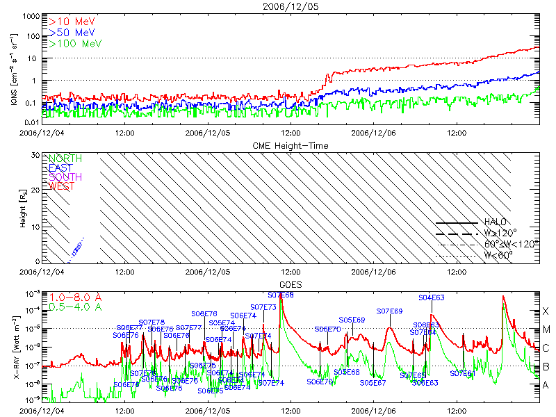
Cite this article
Usoskin, I., Miyake, F., Baroni, M. et al. Extreme Solar Events: Setting up a Paradigm. Space Sci Rev 219, 73 (2023). https://doi.org/10.1007/s11214-023-01018-1
Received:
Accepted:
Published:
DOI: https://doi.org/10.1007/s11214-023-01018-1