
Abstract
Of the existing theoretical formulas for the h-index, those recently suggested by Burrell (J Informetr 7:774–783, 2013b) and by Bertoli-Barsotti and Lando (J Informetr 9(4):762–776, 2015) have proved very effective in estimating the actual value of the h-index Hirsch (Proc Natl Acad Sci USA 102:16569–16572, 2005), at least at the level of the individual scientist. These approaches lead (or may lead) to two slightly different formulas, being based, respectively, on a “standard” and a “shifted” version of the geometric distribution. In this paper, we review the genesis of these two formulas—which we shall call the “basic” and “improved” Lambert-W formula for the h-index—and compare their effectiveness with that of a number of instances taken from the well-known Glänzel–Schubert class of models for the h-index (based, instead, on a Paretian model) by means of an empirical study. All the formulas considered in the comparison are “ready-to-use”, i.e., functions of simple citation indicators such as: the total number of publications; the total number of citations; the total number of cited paper; the number of citations of the most cited paper. The empirical study is based on citation data obtained from two different sets of journals belonging to two different scientific fields: more specifically, 231 journals from the area of “Statistics and Mathematical Methods” and 100 journals from the area of “Economics, Econometrics and Finance”, totaling almost 100,000 and 20,000 publications, respectively. The citation data refer to different publication/citation time windows, different types of “citable” documents, and alternative approaches to the analysis of the citation process (“prospective” and “retrospective”). We conclude that, especially in its improved version, the Lambert-W formula for the h-index provides a quite robust and effective ready-to-use rule that should be preferred to other known formulas if one’s goal is (simply) to derive a reliable estimate of the h-index.
Introduction
Some simple and basic bibliometric indicators, such as the total number of citations C, the total number of publications with at least a number of citations k each, T k , the total number of citations for the t most cited papers, C t , the average number of citations per paper (ACPP), \(m = C/T\) (where, hereafter, T stands for T 0), as well as the h-index (Hirsch 2005; Braun et al. 2006; Schubert and Glänzel 2007; Harzing and van der Wal 2009), are routinely used to measure the relevance and citation impact of journals when computed according to suitable, pre-specified timeframes. In particular, time-limited versions of the ACPP lead to different types of “impact factors”, with possible variants defined according to different pre-specified publication and citation time windows, and also depending on the degree of overlap between these timeframes (synchronous and diachronous impact factors; Ingwersen et al. 2001). Similarly, alternative versions of the h-index have been defined (synchronous and diachronous h-indexes; Bar-Ilan 2010). In general, all these indicators merge information about the number of citations received by a journal within a pre-specified time window—typically a huge amount of data—into a single representative value interpretable as a measure of a journal’s “quality”. Their computation requires knowledge of the entire citation pattern, or at least most of it. In recent years, a certain interest has been shown in developing theoretical models with which to “estimate” one such indicator given the values of certain others. Well-known representative examples are theoretical models with which to obtain the value of the h-index, h:
-
as a function of C (Hirsch 2005),
-
as a function of T (Egghe and Rousseau 2006),
-
as a function of T 1 (Burrell 2013a),
-
as a function of C and T (Glänzel 2006; Iglesias and Pecharroman 2007; Schubert and Glänzel 2007; Bletsas and Sahalos 2009; Egghe et al. 2009; Egghe and Rousseau 2012),
-
as a function of C, T 1 and C 1 Bertoli-Barsotti and Lando (2015);
but also theoretical models with which to estimate C, as a function of h (Petersen et al. 2011), or as a function of m and h (Egghe et al. 2009), or as a function of T and h (Burrell 2013b), and so on. These models—usually based, in their turn, on the assumption of a specific probabilistic model for the citation distribution—may be effective, for instance, when the indicator of interest cannot be obtained directly because it is not accessible, or when the availability of citation data is incomplete. For example, there may be the case in which h is not available but we know C and T (Glänzel 2006; Schubert and Glänzel 2007; Bletsas and Sahalos 2009), or the case in which we have to impute missing values of impact factors using the availability of the h-index as a predictor (Bertocchi et al. 2015).
In particular, in this paper we focus mainly on the problem of obtaining an explicit “universal” formula for estimating the actual value of the h-index. Recently, Burrell (2013b) and Bertoli-Barsotti and Lando (2015) introduced a model that has proved very effective in estimating the actual value of the h-index for individual scientists. More precisely, these approaches lead (or may lead) to two slightly different formulas, being based, respectively, on a “standard” and a “shifted” version of the geometric distribution. In the first part of section ‘Methods’ we present a (functional) equation, based on the geometric distribution, that constitutes a theoretical basis for both these approaches. Indeed, this equation allows us to derive a closed-form estimator of the h-index, expressed as a function of (some of) the above citation metrics. We shall call this estimator, for reasons which will be apparent below, the Lambert-W formula for the h-index.
In the related scientific literature, authors often limit their analysis to the problem of estimating the unknown parameters of a suggested theoretical parametric model for the h-index, under the assumption of knowing the real values of the h-index. Instead, in this paper we consider the more practical (and in a certain sense, opposing) problem of determining the (unknown) h-index on the basis of a ready-to-use formula for it. Then, in our empirical analyses we will use the actual values of the h-index but only to evaluate, a posteriori, the performance of the proposed ready-to-use formulas and not to determine (maybe for interpretative reasons) unknown parameters of a theoretical parametric model. In this paper, we will concentrate on the case of the h-index for journals (Braun et al. 2006). One of the major differences between the cases of an individual scientist and a journal is that, in the latter, the h-index should be computed in a “timed” version, i.e. limited to suitable, usually relatively short, publication and citation time windows. In this regard, it should be noted that a familiar definition such as “a journal has index h if h of its publications each have at least h citations and the other publications each have no more than h citations” is somewhat inaccurate because it does not specify the time windows to be considered for the calculation of h. One of the aims of our study will also be to test the robustness of the formula empirically against different possible choices of (1) length of the time windows and (2) type of approach adopted for analyzing the citation process: “prospective” (diachronous) or “retrospective” (synchronous) (Glänzel 2004). We shall also focus on a comparison of effectiveness between the Lambert-W formula for the h-index and a popular class of alternative models, related to the so-called Glänzel–Schubert formula, that have already been proved to be highly correlated to the h-index.
In the second part of section ‘Methods’ we review the existing literature on the Glänzel–Schubert family of models (and related models) and discuss some problematic aspects linked to the presence of unknown parameters in their expressions. Then, in section ‘Two empirical studies’, we report the results of an empirical comparison between the Lambert-W formula for the h-index and these alternative models, using two different dataset of journals. For this task, we downloaded citation data from the Scopus database on about 100,000 and 20,000 publications, respectively, for the first and the second dataset. Based on the results of our research study, we conclude that the Lambert-W formula for the h-index provides an effective ready-to-use rule that should be preferred to other known formulas if one’s goal is (simply) to derive a reliable estimate of the h-index.
Methods
Models of the relationship between h and other simple metrics based on citation counts
A basic equation connecting h, T and C
A model of a hypothetical equation of the type
is sought, connecting h, T and C. Naturally, we do not assume a deterministic relationship among observed values of h, T and C, rather, we shall determine a “probabilistic” relationship. Indeed, the problem addressed here is that of deriving a formula for predictions. In particular, we try to identify a model that is able to predict one input-term given the other two (e.g. h given T and C, or C given h and T, or, which is the same, C/T given h and T, and so on). A preliminary solution of the functional Eq. (1) can be obtained by “assuming” (which here represents a simple working hypothesis) the geometric distribution (GD) with parameter P,
where p(x) gives the probability of observing x and P, P > 0, represents the expectation of the GD (Johnson et al. 2005, p. 210). Then the value \(n\left( x \right) = Tp\left( x \right)\) expresses the “expected” number of articles with x citations (size-frequency function). Now, since for every k, \(k \in \left\{ {1,2,3, \ldots } \right\}\), \(\sum\nolimits_{x = 0}^{k - 1} {p(x)} = 1 - \left( \frac{P}{1+P}\right)^{k}\), the predicted number of papers with at least k citations is
By definition of the h-index, h, this yields the equation \(\left( {\frac{P}{1 + P}} \right)^{h} - \frac{h}{T} = 0\). Then, assuming \(m = C/T\) as an estimate of the expectation P (see Johnson et al. 2005, Eq. 5.12, p. 211), we derive the following model of functional equation
We note in passing that this model yields, as a byproduct, the formula \(n\left( 0 \right)/{T} = \left( {1 + m} \right)^{ - 1}\) for the “uncitedness factor”, providing proof of the result conjectured by Hsu and Huang (2012) (see also Egghe 2013; Burrell 2013c). This equation represents a theoretical model of the relationship among the h-index, the number of publications T and the ACPP, m. Equation (4) can be solved with respect to any of its arguments. In particular,
-
(a)
Given h and T, we easily obtain an estimate \(P^{*}\) of the expectation P as follows:
$$P^{*} = \frac{{\left( {\frac{h}{T}} \right)^{1/h} }}{{1 - \left( {\frac{h}{T}} \right)^{1/h} }},$$(5)and
-
(b)
Given T and C, we obtain an estimate of h as follows. Equation (4) is equivalent to \(sa^{s} = - T\), where \(a = \frac{m}{1 + m}\) and \(s = - h\). Then, multiplying each side of the latter equation by log a, and substituting \(z = s\log a\), we obtain \(z e^{z} = - T\log a\), which leads immediately to the solution
$$z = W\left( { - T\log a} \right),$$(6)where \(W\left( \cdot \right)\) represents the so-called Lambert-W function (Corless and Jeffrey 2015). Remember that the Lambert-W function is the function W(y) satisfying \(y = W\left( y \right) e^{W\left( y \right)}\), and can be currently computed using mathematical software, for example the Mathematica® 10.0 software package (Wolfram Research, Inc. 2014; it is implemented in the Wolfram Language as “LambertW”), or also using the R statistical computing environment (R Development Core Team 2012).
Hence
$$- h\log \frac{m}{1 + m} = W\left( { - T\log \frac{m}{1 + m}} \right),$$(7)that is, equivalently,
$$h_{W}^{\left( 0 \right)} = \frac{{W\left( {T\log \left( {1 + m^{ - 1} } \right)} \right)}}{{\log \left( {1 + m^{ - 1} } \right)}},$$(8)where we have adopted a new symbol for differentiating the “predicted” h-index, \(h_{W}^{\left( 0 \right)}\), from the actual value h of the h-index. Note that the GD approach has been previously suggested by Burrell (2007, 2013b, 2014) but without giving an explicit formula, in closed form, for the estimation of the h-index.
An equation connecting h, T 1 and C
As a general rule, one should expect that knowledge of other (i.e., other than m and T) simple summary statistics of the raw citation data will help increase the precision of the h-index estimate. Indeed, if we also assume that we know T 1, a modified version of the above formulas can be easily introduced by taking the shifted-geometric distribution (SGD) with parameter Q
where p(y) represents the probability of observing the number of citations y of a paper cited at least once, and Q, Q > 1, represents the expectation of the SGD. Since for every k, \(k \in \left\{ {1,2,3, \ldots } \right\}\), \(\sum\nolimits_{y = 1}^{k} {p\left( y \right)} = 1 - \left( {\frac{Q - 1}{Q}} \right)^{k}\), then \(T_{1} \left( {\frac{Q - 1}{Q}} \right)^{k}\) represents the number of papers with at least k + 1 citations. Then, assuming \(m_{1} = {C \mathord{\left/ {\vphantom {C {T_{1} }}} \right. \kern-0pt} {T_{1} }}\), the average number of citations of articles that have been cited at least once, as a proxy for the expectation Q, we derive the following functional equation
This equation can be solved with respect to any of its arguments. In particular,
-
(c)
Given h and T 1, we obtain
$$Q^{*} = \left( {1 - \left( {\frac{h}{{T_{1} }}} \right)^{{{1 \mathord{\left/ {\vphantom {1 {\left( {h - 1} \right)}}} \right. \kern-0pt} {\left( {h - 1} \right)}}}} } \right)^{ - 1}$$(11)and
-
(d)
Given T 1 and C, and following a completely analogous sequence of steps as in the above point (b), we obtain the estimate of h
$$h_{W}^{\left( 1 \right)} = \frac{ - 1}{{\log \left( {1 - m_{1}^{ - 1} } \right)}} \cdot W\left( {\frac{{T_{1} }}{{1 - m_{1}^{ - 1} }} \cdot \log \left( {1 - m_{1}^{ - 1} } \right)} \right).$$(12)
A formula for the h-index, as a function of T 1, C and C 1
If we also know the total number of citations of the most cited paper, C 1, we can hope to improve the accuracy of the above formula \(h_{W}^{\left( 1 \right)}\) further. Indeed, with the use of the trimmed mean—that is, the sample mean obtained omitting the most highly cited paper—\(\tilde{m}_{1} = {{\left( {C - C_{1} } \right)} \mathord{\left/ {\vphantom {{\left( {C - C_{1} } \right)} {\left( {T_{1} - 1} \right)}}} \right. \kern-0pt} {\left( {T_{1} - 1} \right)}}\) instead of m 1, we obtain a modified (improved) version of the above formula, which we shall define \(\tilde{h}_{W}^{\left( 1 \right)}\),
As is well known, citation distributions are highly skewed; hence the sample mean is distorted by extreme values. In particular, the presence of individual highly-cited papers tends to overestimate C, and consequently \(h_{W}^{\left( 1 \right)}\), in comparison to the true h-index—that is clearly insensitive to a single very highly cited paper. In this sense, the use of a trimmed mean is simply a technique for reducing this possible bias.
To summarize, we have: \(h_{W}^{\left( 0 \right)} = h_{W}^{\left( 0 \right)} \left( {C,T} \right)\) or also, equivalently, \(h_{W}^{\left( 0 \right)} = h_{W}^{\left( 0 \right)} \left( {T,m} \right)\), and \(\tilde{h}_{W}^{\left( 1 \right)} = \tilde{h}_{W}^{\left( 1 \right)} \left( {C,C_{1} ,T_{1} } \right)\) or also, equivalently, \(\tilde{h}_{W}^{\left( 1 \right)} = \tilde{h}_{W}^{\left( 1 \right)} \left( {T_{1} ,\tilde{m}_{1} } \right)\). We shall refer to these formulas as Lambert-W formulas for the h-index, respectively, in a “basic”, \(h_{W}^{\left( 0 \right)}\), and an “improved” version, \(\tilde{h}_{W}^{\left( 1 \right)}\). The formula \(\tilde{h}_{W}^{\left( 1 \right)}\) has been considered elsewhere Bertoli-Barsotti and Lando (2015) for the estimation of the h-index for individual scientists.
Theoretical parametric models for the h-index related to the Glänzel–Schubert formula
A well-known alternative “theoretical model of the dependence of the citation h-index on the sample size and the sample’s mean citation rate” (Schubert et al. 2009) is the one proposed by Schubert and Glänzel (2007), who noted that the h-index is approximately proportional to “a power function of the sample size and the sample mean”, namely to the function \(m^{\eta } T^{1 - \eta }\) (Schubert et al. 2009; see also Glänzel 2007, 2008). In applications, this fact has given rise to a plethora of “variants”, as possible parametric models for the h-index. It is useful to distinguish each of them with the following nine cases.
-
(a)
Iglesias and Pecharroman (2007) derived the following one-parameter family of models of the h-index:
$$h_{\text{IP}} \left( \eta \right) = \left( {\frac{2\eta - 1}{\eta }} \right)^{\eta } m^{\eta } T^{1 - \eta } ,$$(14)where \(\eta > 0.5\) (the formula was reported by Iglesias and Pecharroman with parameter \({{\left( {1 - \eta } \right)} \mathord{\left/ {\vphantom {{\left( {1 - \eta } \right)} \eta }} \right. \kern-0pt} \eta }\)). Glänzel (2008) estimated this model in an empirical comparative study of h-index for journals. He found that the estimate of the power parameter depends on the length of the citation window considered. In particular, he found that the formula \(h_{\text{IP}} \left( {2/3} \right)\) (α = 2 in his notation, which corresponds to η = 2/3 in ours) is appropriate “for small windows comprising an initial period of about 3 years after publication”.
-
(b)
From the above model, Iglesias and Pecharroman (2007) also obtained, for η = 2/3, the ready-to-use formula:
$$h_{\text{IP}} \left( {2/3} \right) = 4^{ - 1/3} m^{2/3} T^{1/3}$$(15)(see also Panaretos and Malesios 2009; Vinkler 2009, 2013; Ionescu and Chopard 2013).
-
(c)
By starting from a continuous probability distribution—a Pareto distribution of the second kind, \(P\left( {II} \right)\left( {\sigma ,\theta } \right)\) (Johnson et al. 1994, p. 575; Arnold 1983, p. 44), also known as the Lomax distribution (Lomax 1954), where \(\sigma^{\theta } \left( {\sigma + x} \right)^{ - \theta } ,\;\theta > 0,\;\sigma > 0\), represents the probability of observing a number greater than x, x > 0—and estimating its expectation \(\sigma \left( {\theta - 1} \right)^{ - 1}\) (that exists if \(\theta > 1\)) by the sample mean m, Schubert and Glänzel (2007) (see also Glänzel 2006) derived a slightly more general two-parameter model:
$$h_{\text{G}} \left( {\eta ,\gamma } \right) = \gamma m^{\eta } T^{1 - \eta }$$(16)here defined as also reported by Bletsas and Sahalos (2009); see their Eq. (4)), as an approximate (and generalized) solution of the equation
$$Tm^{\theta } \left( {\theta - 1} \right)^{\theta } \left( {\sigma + h} \right)^{ - \theta } = h,$$(17)where \(\theta = \eta \left( {1 - \eta } \right)^{ - 1}\). In words, model (16) states that “the h-index can be approximated by a power function of the sample size and the sample mean” (Schubert et al. 2009). It is important to note that the model \(h_{G} \left( {\eta ,\gamma } \right)\) is similar to but different from the above model \(h_{\text{IP}} \left( \eta \right)\), because in the former the proportionality constant is not merely a function of the power parameter η, while in the latter γ represents a free parameter. This gives rise to a more flexible model. Malesios (2015) estimated the parameters of model (16) in a study on 134 journals in the field of ecology and 54 journals in the field of forestry sciences. He obtained the best fit, respectively, with the estimates (0.64, 0.7) and (0.66, 0.78) for the pair (η, γ) (in our parameterization).
-
(d)
The above Pareto distribution of the second kind \(P\left( {II} \right)\left( {\sigma ,\theta } \right)\) has also recently become known as the Tsallis distribution (Tsallis and de Albuquerque 2000). More specifically, with reparameterization \(\theta = \left( {q - 1} \right)^{ - 1}\) and \(\sigma = \left( {q - 1} \right)^{ - 1} \lambda^{ - 1} ,\;q > 1,\;\lambda > 0\), the probability of observing a number greater than x, x > 0, becomes equal to \(\left( {1 + \lambda \left( {q - 1} \right)x} \right)^{{ - \frac{1}{q - 1}}}\) (see Bletsas and Sahalos 2009; Shalizi 2007). Bletsas and Sahalos (2009) suggest obtaining an estimate of the h-index as the numerical solution of the Eq. (17), that is
$$T\left( {m\frac{2 - q}{q - 1}} \right)^{{\frac{1}{q - 1}}} \left( {m\frac{2 - q}{q - 1} + h} \right)^{{\frac{1}{1 - q}}} = h,$$(18)for a pre-specified fixed value of the unknown parameter q. Let us call \(h_{\text{BS}} = h_{\text{BS}} \left( q \right)\) the (implicit) solution of Eq. (18). It is important to stress that, unlike all the other estimators of h-index considered in the present study, a closed-form expression for h T does not exist. Nevertheless, in an empirical application to a set of electrical engineering journals, Bletsas and Sahalos (2009) found a very good fit between measured and estimated values of the h-index, assuming Tsallis distribution with parameter q = 1.5 and q = 1.6. It is interesting to note that these values correspond, respectively, to η = 2/3 and η = 0.625, since \(\eta = q^{ - 1}\).
-
(e)
For a special choice of the power parameter (η = 2/3 in the present parameterization) in model (16), Schubert and Glänzel (2007) derived the celebrated one-parameter model
$$h_{\text{SG}} \left( \gamma \right) = \gamma C^{2/3} T^{ - 1/3} = \gamma m^{2/3} T^{1/3} ,$$(19)also known as the Glänzel–Schubert model of the h-index. This model has been widely used (mainly for interpretative purposes—i.e. to provide a better understanding of the “mathematical properties” of the h-index) because several empirical studies suggest the existence of a strong correlation between h-index and \(m^{2/3} T^{1/3}\). Its drawback (as with model (16)) is obviously that the value of the proportionality constant γ is unknown. Certainly, this parameter can be determined (ex post) empirically, but it is likely to vary from case to case (Prathap 2010a; Alguliev et al. 2014). Then, as a ready-to-use formula for estimating the h-index a priori, the Glänzel–Schubert model is in fact unusable. Sometimes researchers find an ex post least square estimate of the parameter γ, starting from known values of the h-index. In different contexts, and for different datasets, the estimate of the γ parameter has been found to vary appreciably, in that it turns out to range approximately from 0.7 to 0.95. Indeed, for example, Schubert and Glänzel (2007) found, for γ, the estimates 0.73 and 0.76, in a study on the h-index for journals, for two different sets of journals, while Csajbók et al. (2007) found an estimate of γ of 0.93 in a macro-level analysis of the h-index for countries. Instead, other authors, among them Annibaldi et al. (2010), Bouabid et al. (2011) and Zhao et al. (2014), have found values of around 0.8. In quite different contexts (partnership ability and h-index for networks) Schubert (2012) and Schubert et al. (2009) have estimated the parameter γ of the model \(h_{\text{SG}} \left( \gamma \right)\), obtaining values within the range 0.6–0.96.
-
(f)
In the absence of a specific value of the proportionality constant γ, researchers sometimes decide to set γ equal to a fixed arbitrary value γ 0, obtaining a ready-to-use formula
$$h_{\text{SG}} \left( {\gamma_{0} } \right) = \gamma_{0} m^{2/3} T^{1/3} .$$(20)In the framework of the analysis of the h-index for journals, ready-to-use formulas for estimating the h-index with the formula \(h_{\text{SG}} \left( {\gamma_{0} } \right)\) have been adopted, for example, by Bletsas and Sahalos (2009), with the choice \(\gamma_{0} = 0.75\). Instead, for example, Ye (2009, 2010) and Elango et al. (2013) adopted the rule to set \(\gamma_{0} = 0.9\) for journals and \(\gamma_{0} = 1\) for other sources. Abbas (2012) and Vinkler (2013) also adopted the choice \(\gamma_{0} = 1\). It is worth noting that the latter value leads to the formula \(h_{\text{SG}} \left( 1 \right)\), which coincides with the so-called p-index defined by Prathap (2010b). Finally, note that \(h_{\text{SG}} \left( {4^{ - 1/3} } \right) = h_{\text{IP}} \left( {2/3} \right)\).
-
(g)
As noted above, empirical analyses suggest a “strong linear correlation” between the h-index and the function \(m^{\eta } T^{1 - \eta }\) (Schubert and Glänzel 2007; Glänzel 2007; Schreiber et al. 2012; Malesios 2015). Strictly speaking, this only means that when h is plotted against \(m^{\eta } T^{1 - \eta }\), the data fall fairly close to a straight line. In other terms, h is approximately equal to \(\delta + \gamma m^{\eta } T^{1 - \eta }\), for suitable choices of the parameters δ and γ. Indeed, the following three-parameter model has been considered in literature (see Bador and Lafouge 2010)
$$h_{\text{BL}} \left( {\delta ,\gamma ,\eta } \right) = \delta + \gamma m^{\eta } T^{1 - \eta } .$$(21)In a comparative analysis of two samples of 50 journals (taken from the ‘‘Pharmacology and Pharmacy’’ and ‘‘Psychiatry’’ sections of the Journal Citation Reports 2006), Bador and Lafouge (2010) obtained the LS estimates of the parameters δ and γ for different fixed values of the power parameter η (values of “α close to 2”, in their parameterization, where \(\eta = {\alpha \mathord{\left/ {\vphantom {\alpha {\left( {\alpha + 1} \right)}}} \right. \kern-0pt} {\left( {\alpha + 1} \right)}}\)). Their best estimates of the proportionality constant γ ranged from 0.7 to 0.8, with an intercept point always very close to 1. Based on these results, \(h_{\text{BS}} \left( {\eta ,\gamma } \right)\) and a fortiori \(h_{\text{SG}} \left( \gamma \right)\), underestimate the h-index.
-
(h)
For the particular choice of the power parameter η = 2/3 in the above model \(h_{\text{BL}} \left( {\delta ,\gamma ,\eta } \right)\), we obtain the two-parameter model
$$h_{\text{TAB}} \left( {\delta ,\gamma } \right) = \delta + \gamma \cdot m^{2/3} T^{1/3} .$$(22)This model directly generalizes the above Glänzel–Schubert model \(h_{\text{SG}} \left( \gamma \right)\) by introducing a free intercept parameter, δ. Tahira et al. (2013) tested this model in a scientometric analysis of engineering in Malaysian universities. They found the estimates δ = −0.28 and γ = 0.97.
-
(i)
Finally, by assuming a linear dependence between the h-index and the function \(m^{\eta } T^{1 - \eta }\) in a double logarithmic axis plot (log–log plot), one may define the following three-parameter model (see Radicchi and Castellano 2013)
$$h_{RC} \left( {{\varrho },\varphi ,\eta } \right) = {\varrho }\left( {m^{\eta } T^{1 - \eta } } \right)^{\varphi } .$$(23)Indeed, after taking logs, this corresponds to a regression relationship between log h and the linear model \(\xi + \varphi \cdot \log \left( {m^{\eta } T^{1 - \eta } } \right)\), where \({\varrho } = e^{\xi }\). Needless to say, model \(h_{\text{RC}}\) is similar to but essentially different from the above models (a)–(h). Radicchi and Castellano (2013) analyzed the scientific profile of more than 30,000 researchers. They found a good linear correlation, in a log–log plot, between the true h-index and the values given by the model \(h_{\text{RC}} \left( {{\varrho },\varphi ,\eta } \right)\). Using this relationship, they obtained, in particular, the least square estimate of the parameter η: \(\hat{\eta } = 0.41\). It is quite puzzling to observe that the solution reached by Radicchi and Castellano is out of the parameter space of all the above models (η > 0.5).
Two empirical studies
A first dataset of journals
Journal selection
The Research Evaluation Exercise for the period 2011–2014 named “Valutazione della Qualità della Ricerca 2011–2014” (hereinafter VQR) is a national research assessment exercise organized under the aegis of the Italian Ministry of Education, University and Research for evaluating and ranking all Italian scientific institutions (typically, all national universities and research centers), on the basis of the quality of their research outcomes. The results obtained are particularly important because they determine the allocation of government funding to Italian universities. The VQR is carried out under the responsibility of a National Agency for the Evaluation of University and Research, the “Agenzia Nazionale di Valutazione del Sistema Universitario e della Ricerca” (ANVUR), and is organized with reference to 14 different academic fields, or Areas. The research assessment is actually conducted by Groups of Evaluation Experts (GEV, in the Italian acronym), one for each Area. For our first empirical analysis, we consider the so-called Area 13—Scienze economiche e statistiche—Economics and Statistics. The evaluation of each researcher is based on the quality of his/her research outcomes published during the period 2011–2014. As a general rule, the evaluation of a research product for Area 13 is made at journal-level. This means that journal bibliometric indicators are used as surrogate measures to quantify the quality of each individual research product (published in that journal). For this purpose, a list of “relevant” journals for Area 13 has been compiled by the corresponding GEV (the so-called GEV 13) and suitable journal-based metrics are extracted to this end from three sources, that is: Web of Science (WoS), Scopus, and Google Scholar (GS). The full list of the “relevant” journals for Area 13 includes 2717 journals and may be found on the ANVUR website (www.anvur.org). Each journal on the Area 13 list was individually assigned to one of five sub-areas, among them “Statistics and Mathematical Methods” (S&MM). For the purpose of our case study, we selected a somewhat homogeneous list of journals using the following steps:
-
(a)
we considered all and only the journals (568 journals) belonging to the sub-area S&MM;
-
(b)
to facilitate possible comparisons between databases, the journals selected were subsequently restricted to only those (253) journals indexed by all three databases: WoS, Scopus and GS;
-
(c)
we excluded 15 journals with incomplete issues within the period under investigation, 2010–2014;
-
(d)
finally, in order to preserve the homogeneity of the sample, we excluded 6 journals with a “too large” number of published papers (more than 2000) and 1 journal that publishes only online.
Our final sample included 231 journals. According to the Scopus classification, these journals belong to a number of different “Subject Areas”. Table 1 shows the “Subject Areas” in which the 231 journals selected from the S&MM list are placed by Scopus (it should be recalled that Scopus classifies journal titles into 27 major thematic categories and a journal may belong to more than one category).
Estimating the h-index
After selecting the S&MM list of journals, we retrieved citation data from the Scopus database. According to the VQR time-span, we considered all documents within the publication window of 5 years (2010–2014) (in fact GEV13 considers the 5-year Google Scholar’s h-index, for the period 2010–2014) and the citations that these items received until the time of accessing the database (last week of December 2015). This means a 6-year citation window, 2010–2015, over a 5-year publication window: 2010–2014. Harzing and van der Wal (2009) considered similar timeframes in a study on a set of journals in the area of economics and business. Overall, the dataset obtained included 99,409 publications receiving (until December 2015) a total of 485,628 citations. The complete list of the 231 journals in the S&MM dataset is reported in Table 2, where each journal is identified by its ISSN code. For each journal, we manually computed, on the basis of the citations downloaded, the actual value h of the h-index, as: the largest number of papers published in the journal between 2010 and 2014 and which obtained at least h citations each, from the time of publication until December 2015. Table 2 reports, for each journal, the h-index, h, and its estimates, obtained (1) with the Lambert-W formulas for the h-index, \(h_{W}^{\left( 0 \right)}\), \(\tilde{h}_{W}^{\left( 1 \right)}\), and, as a comparison, (2) with the Glänzel–Schubert formula, \(h_{\text{SG}} \left( {\gamma_{0} } \right)\), for different values of the proportionality constant γ 0, namely, 0.63, 0.7, 0.8, 0.9, 1 (note that \(\gamma_{0} = 0.63 = 4^{ - 1/3}\) identifies formula \(h_{\text{IP}} \left( {2/3} \right)\)), and (3) by means of a numerical solution \(h_{\text{BS}} \left( {q_{0} } \right)\) of Eq. (18), for different values of q 0, namely, 1.2, 1.4, 1.6. Table 2 also reports: the total number of citations, C; the total number of publications, T; the total number of publications cited at least once, T 1; the total number of citations of the most cited paper, C 1. To facilitate comparisons, \(h_{W}^{\left( 0 \right)} ,\;\tilde{h}_{W}^{\left( 1 \right)} ,\;h_{\text{SG}} \left( {\gamma_{0} } \right),\;{\text{and}}\;h_{\text{BS}} \left( {q_{0} } \right)\) have all been rounded to the nearest integer to produce numbers in the same range of values as the h-index.
A second dataset of journals
Journal selection
We also analyzed a second dataset, based on the citation data of the top 100 journals, within the Scopus subject area of “Economics, Econometrics and Finance”, ranked according to the Scopus journal impact factor, i.e. the Impact per Publication (IPP) 2014. The list (let us call it the EE&F list) may be found at http://www.journalindicators.com and it consists of journals with a minimum number of 50 publications. We recall that the IPP 2014 of a journal is basically the average number of citations received by papers published in 2014 (registered in the Scopus database), to papers published by the same journal from 2011 until 2013. In particular, Scopus takes account of the following types of citable items and citing sources: articles, reviews, and conference papers. All other documents (e.g. notes, letters, articles in press, erratum, etc.) are excluded from the computation. We downloaded from Scopus the citation data of all 100 journals on the aforementioned list during the last week of April, 2016. The dataset obtained included 19,889 publications receiving a total of 74,096 citations (during 2014). The complete list of these journals is reported in Table 3, where each journal is identified by its ISSN code. Differently from above, we excluded all non-citable items (e.g. notes, etc.) in order to obtain sets of publications as close as possible to those employed for the computation of IPPs by Scopus. Once the set of papers for each journal has been selected, it is possible to request a citation report (“view citation overview”) and download the citations per paper received in the year 2014: that is, all and only the citations needed for the computation of the IPP 2014. In fact, we found some positive differences between the actual values of \(m = C/T\), with an average value over all 100 journals of 3.8, and the official IPPs 2014, with an average value of 3. These differences may be due to: (1) a delayed update of the database (the IPPs were published by Scopus in June 2015), and (2) a larger set of citing sources and documents (with Scopus, it is not possible to limit the citation report to particular citing sources or documents). Similar differences between official and observed values have been found and discussed, for instance, by Leydesdorff and Opthof (2010), Stern (2013) and Seiler and Wohlrabe (2014). Nonetheless, in this case the ACPP \(m = C/T\) should, theoretically, represent a 3-year synchronous impact factor for the year 2014 (Ingwersen et al. 2001; Ingwersen 2012) in that we considered only citations received during 2014 of papers published within the previous 3 years. For each journal, we manually computed the actual value h of the h-index as the largest number of papers published in the journal between 2011 and 2013 and which obtained at least h citations each in the year 2014. Ultimately, we obtained a synchronous h-index (Bar-Ilan 2010), for a 1-year citation window.
Estimating the h-index
In the same way as above, for each journal we manually computed the actual value h of the h-index. Table 3 reports, for each journal, the h-index, h, and the other indicators also considered in Table 2, namely \(h_{W}^{\left( 0 \right)}\), \(\tilde{h}_{W}^{\left( 1 \right)}\), \(h_{\text{SG}} \left( {\gamma_{0} } \right)\), for \(\gamma_{0} = 0.63, 0.7, 0.8, 0.9, 1\), the numerical solution \(h_{\text{T}} \left( {q_{0} } \right)\) of Eq. (18), for different values of q 0, namely \(q_{0} = 1.2, 1.4, 1.6\), as well as the simple basic metrics C, T, T 1 and C 1.
Discussion and conclusion
The h-index is, today, one of the tools most commonly used to rank journals (Braun et al. 2006; Vanclay 2007, 2008; Schubert and Glänzel 2007; Bornmann et al. 2009; Harzing and van der Wal 2009; Liu et al. 2009; Hodge and Lacasse 2010; Bornmann et al. 2012; Mingers et al. 2012; Xu et al. 2015). Indeed, its value is currently provided by all the three major citation databases, WoS, Scopus and GS. In an earlier study (Bertoli-Barsotti and Lando 2015) the Lambert-W formula for the h-index \(\tilde{h}_{W}^{\left( 1 \right)}\) was proved to be a good estimator of the h-index for authors. In this paper, we have extended the empirical study to the case of the h-index for journals. One of the major differences between the case of an individual scientist and that of a journal, for the computation of the h-index, is the role played by publication and citation time windows, and the approach adopted for the analysis and interpretation of the citation process (“prospective” vs “retrospective”; Glänzel 2004). As stressed by Braun et al. (2006): “The journal h-index would not be calculated for a “life-time contribution”, as suggested by Hirsch for individual scientists, but for a definite period”. In fact, “Hirsch did not limit the period in which the citations were received” (Bar-Ilan 2010). Unlike the case of individual scientists, and in view of a comparative assessment, calculations of a journal’s h-index must be timed (note that a notion of “timed h-index” has also been recently introduced by Schreiber (2015), for the case of individual scientists), i.e. it must be referred to standardized time periods of journal coverage, for example of 2, 3 or 5 years, as is usually done for the computation of the impact factor, in order to limit the typical size-dependency of the h-index—that is, its dependency on the total number of publications (an indicator is said to be size-dependent if it never decreases when new publications are added, Waltman 2016). A journal’s “impact factor” is essentially a time-limited version of the average number of citations by papers published in the journal in a given period of time. Several types of “impact factors” may be defined, depending on different time windows considered for publication and citation data and, possibly, different approaches to the analysis of the citation process, leading to synchronous or diachronous impact factors (Ingwersen et al. 2001; Ingwersen 2012). In its WoS form, the publication window is 2 years (defining the 2-year Impact Factor, IF) or 5 years (defining the 5-year Impact Factor, IF5), while Scopus adopts a 3-year publication window for its IPP. In all these cases, the impact factor is computed in a synchronous mode, i.e. the citations used for the calculation are all received during the same fixed period—1 year, in these cases.
In this paper, we first presented the Lambert-W formula for the h-index in two versions (differing on the basis of the various citation metrics on which they depend), a basic version and an improved version, respectively \(h_{W}^{\left( 0 \right)}\) and \(\tilde{h}_{W}^{\left( 1 \right)}\). Then we tested, by means of an empirical study, their efficiency and effectiveness, as well as:
-
1.
that of another popular theoretical model for the h-index that has been successfully applied elsewhere to the same type of application, i.e. the Glänzel–Schubert formula, \(h_{\text{SG}} \left( {\gamma_{0} } \right)\), for different values of the free parameter γ 0, and secondly,
-
2.
that given by the numerical solution \(h_{\text{BS}} \left( {q_{0} } \right)\) of Eq. (18), for different values of the free parameter q 0.
We compared the performances of these formulas as estimators of the h-index—in particular, in terms of accuracy and robustness—with an empirical study conducted on two different samples of journals. We computed the h-index manually, on the basis of citations downloaded. In our empirical study, in the first dataset (S&MM), the ACPP \(m = C/T\) can be interpreted as a diachronous impact factor (Ingwersen et al. 2001; Ingwersen 2012), because for each paper the citations are counted from the moment of publication until the time of accessing the database (as in the case of individual scientists). More specifically, we computed an “impact factor” involving a 6-year citation window over a 5-year publication window. As to be expected, due to the larger citation window, we obtained, for all 231 journals, the averages of 4.4 and 1.5 respectively for m and IF5{2014}, the traditional 5-year impact factors 2014, as published by WoS in its Journal Citation Report. Moreover, we also observed a high level of Pearson correlation, ρ, between m and IF5{2014}, that is: \(\rho \left( {m,IF5\left\{ {2014} \right\}} \right) = 0.87\) (quite similar to that observed between IF5{2014} and IF{2014}, the WoS 2-year and impact factors 2014, that is: \(\rho \left( {IF\left\{ {2014} \right\},IF5\left\{ {2014} \right\}} \right) = 0.90\)). Instead, in the second dataset (EE&F), m can be interpreted as a 3-year impact factor in its ordinary synchronous version, as computed by Scopus. Hence, following the terminology of Bar-Ilan (2010, 2012), we obtained a diachronous and a synchronous h-index, respectively, in the first and second empirical study. To evaluate the measure of fit of an estimate of the h-index, say \(\hat{h}_{j}\) (rounded to the nearest natural number), with respect to the exact value h j , we computed the absolute relative error \({\text{ARE}}_{j} = \left| {{{\left( {\hat{h}_{j} - h_{j} } \right)} \mathord{\left/ {\vphantom {{\left( {\hat{h}_{j} - h_{j} } \right)} {h_{j} }}} \right. \kern-0pt} {h_{j} }}} \right|\) and the squared relative error \({\text{SRE}}_{j} = \left( {{{\left( {\hat{h}_{j} - h_{j} } \right)} \mathord{\left/ {\vphantom {{\left( {\hat{h}_{j} - h_{j} } \right)} {h_{j} }}} \right. \kern-0pt} {h_{j} }}} \right)^{2}\) for each journal j, j = 1,…,J. Then, as a criterion with which to assess the overall quality of the various estimators considered in the paper, we computed the mean absolute relative error, \({\text{MARE}}\left( {\hat{h}} \right) = \sum\nolimits_{j = 1}^{J} {{{{\text{ARE}}_{j} } \mathord{\left/ {\vphantom {{{\text{ARE}}_{j} } J}} \right. \kern-0pt} J}}\) and the root mean squared relative error \({\text{RMSRE}}\left( {\hat{h}} \right) = \sqrt {\sum\nolimits_{j = 1}^{J} {{{{\text{SRE}}_{j} } \mathord{\left/ {\vphantom {{{\text{SRE}}_{j} } J}} \right. \kern-0pt} J}} }\), for each estimator.
-
1.
As expected, the Pearson correlation between the actual value h of the h-index and each of its estimates \(h_{W}^{\left( 0 \right)}\), \(\tilde{h}_{W}^{\left( 1 \right)}\) and \(h_{\text{SG}} \left( {\gamma_{0} } \right)\), was very high, for both S&MM and EE&F datasets. In particular, this confirms previous empirical results concerning the formula \(h_{\text{SG}}\) (see Schubert and Glänzel 2007; Glänzel 2007). Indeed, ρ always exceeded 0.97. More specifically, we found the following: for the S&MM dataset, \(\rho ( {h,h_{W}^{( 0 )} }) = 0.97\) and \(\rho ( {h,\tilde{h}_{W}^{( 1 )} } ) = \rho ( {h,h_{\text{SG}} } ) = 0.98\); for the EE&F dataset,\(\rho ( {h,h_{W}^{( 0 )} } ) = \rho ( {h,h_{\text{SG}} } ) = 0.97\) and \(\rho ( {h,\tilde{h}_{W}^{( 1 )} } ) = 0.98\). Nevertheless, as can be seen from Figs. 2 and 4, a high correlation does not specifically identify a “good” estimator for the h-index. Formula \(\tilde{h}_{W}^{( 1 )}\) yielded similar levels of correlation, but a much lower level of MARE, see Figs. 1 and 3 (be aware that the figures refer to non-rounded values of the estimates). Note that the correlation between the h-index and \(h_{\text{SG}} \left( {\gamma_{0} } \right)\) does not depend on the unknown value of \(\gamma_{0}\), while, at the same time, the MARE of \(h_{SG} \left( {\gamma_{0} } \right)\) depends heavily on the choice of \(\gamma_{0}\). As can be seen from Table 4, at its best (among the values of \(\gamma_{0}\) tested), the error of \(h_{SG} \left( {\gamma_{0} } \right)\) reached its minimum (in terms of both MARE and RMSRE), for \(\gamma_{0} = 0.9\), for the dataset S&MM, while for the EE&F dataset the error of \(h_{SG} \left( {\gamma_{0} } \right)\) is at its minimum for a slightly different value of γ 0, i.e. γ 0 = 0.8. This confirms that, for fixed values of γ 0, the effectiveness of the formula may depend on the length of the citation window considered (Glänzel 2008) and, finally, that there is no “universal” optimal value for the constant γ 0 in the formula \(h_{\text{SG}} \left( {\gamma_{0} } \right)\). Instead, for both datasets, the formula \(\tilde{h}_{W}^{\left( 1 \right)}\) gives similar, and even smaller, levels of error (in terms of both MARE and RMSRE).
Fig. 1 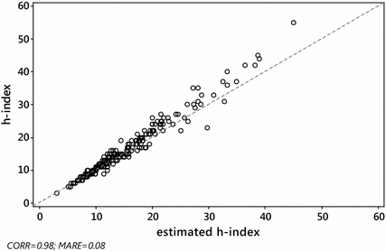
S&MM dataset: scatterplot of h versus \(\tilde{h}_{W}^{\left( 1 \right)}\). Pearson correlation \(\rho \left( {h,\tilde{h}_{W}^{\left( 1 \right)} } \right) = 0.98\), \({\text{MARE}}\left( {\tilde{h}_{W}^{\left( 1 \right)} } \right) = 0.08\). The dashed line is identity, so ideally all the points should overlie this line
Fig. 2 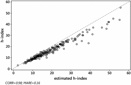
S&MM dataset: scatterplot of h vs Glänzel–Schubert formula \(h_{\text{SG}} \left( 1 \right)\). Pearson correlation \(\rho \left( {h,h_{\text{SG}} \left( 1 \right)} \right) = 0.98\), \({\text{MARE}}\left( {h_{\text{SG}} \left( 1 \right)} \right) = 0.16\). The dashed line is identity, so ideally all the points should overlie this line
Fig. 3 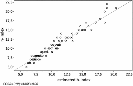
EE&F dataset. Scatterplot of h versus \(\tilde{h}_{W}^{\left( 1 \right)}\). Pearson correlation \(\rho \left( {h,\tilde{h}_{W}^{\left( 1 \right)} } \right) = 0.98\), \({\text{MARE}}\left( {\tilde{h}_{W}^{\left( 1 \right)} } \right) = 0.05\). The dashed line is identity, so ideally all the points should overlie this line
Fig. 4 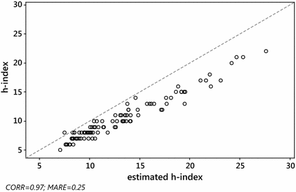
EE&F dataset: versus Glänzel–Schubert formula \(h_{\text{SG}} \left( 1 \right)\). Pearson correlation \(\rho \left( {h,h_{\text{SG}} \left( 1 \right)} \right) = 0.97\), \({\text{MARE}}\left( {h_{\text{SG}} \left( 1 \right)} \right) = 0.25\). The dashed line is identity, so ideally all the points should overlie this line
Table 4 Relative accuracy, computed in terms of MARE and RMSRE (in italic), of different estimators of the h-index. For each dataset, the smallest error is indicated by a boldface number -
2.
The approach that consists of obtaining the numerical solution \(h_{\text{BS}} \left( {q_{0} } \right)\) of Eq. (18) was also considered. We tentatively tested this method for nine different values of the free parameter q between 1 and 2, i.e. q 0 = 1.1, 1.2,…,1.9. As expected, the resulting estimates were more or less accurate depending on the set value of q 0. Of the nine values of q 0 tested, the smallest estimation error was obtained for a q 0 value equal to around 1.4 (MARE = 0.065; RMSRE = 0.094), for the S&MM dataset, and for a q 0 value equal to around 1.2 (MARE = 0.058; RMSRE = 0.093) for the EE&F dataset (see Table 4). Ultimately, h T was found to be the most accurate estimator (if one takes q 0 = 1.4), of those included in Table 4, for the S&MM dataset and the third best (if one takes q 0 = 1.2), for the EE&F dataset. Overall, the errors are not dramatically different in the range of q between 1.2 and 1.6, and then a value of q 0 = 1.5, also tested by Bletsas and Sahalos (2009), may be a good compromise solution. The Pearson correlation between the actual value h of the h-index and its estimate \(h_{\text{BS}} \left( {q_{0} } \right)\) varies slightly according to the selected value of q 0, but it is still very high: in particular, for q 0 = 1.5, we obtain \(\rho \left( {h,h_{\text{BS}} \left( {q_{0} } \right)} \right) = 0.98\) for the S&MM dataset and \(\rho \left( {h,h_{\text{BS}} \left( {q_{0} } \right)} \right) = 0.96\) for the EE&F dataset. Hence, overall, the method may lead to a very good fit, but it has two main drawbacks. First, the expression of \(h_{\text{BS}} \left( {q_{0} } \right)\) is not given by any explicit formula. Second, this method continues to suffer from the problem of the conventional choice of an unknown parameter, in that we do not know a priori the value of the parameter q that will yield the “smallest” estimation error.


In conclusion, basically, the same type of equation (see Eqs. 4, 10), describes the relationship between the h-index and other simple citation metrics. The Lambert-W formula for the h-index works well (also) for estimating the h-index for journals—especially in its improved version (13). As can be deduced from our empirical study, this still holds true for different scientific areas, for different time windows for publication and citation, for different types of “citable” documents, and for different approaches to the analysis of the citation process (“prospective” vs “retrospective”; Glänzel 2004). At the same time, the Glänzel–Schubert class of models seems to be much less robust and reliable as an estimator of the h-index, because its accuracy closely depends on a conventional choice of one or more unknown parameters. We may accordingly conclude that \(h_{W}^{\left( 0 \right)}\) and \(\tilde{h}_{W}^{\left( 1 \right)}\) are quite effective “universal” (in the sense that they are ready-to-use) informetric functions that work well for estimating the h-index, for a sufficiently wide range of values. Indeed, our empirical analysis, though preliminary, suggests that the fit is very good, at least for the datasets that we studied, and for values of its arguments that are not too large, namely, h < 40, T < 2000 and m < 20, which may be considered standard values for the cases of both and scientists journals within time-spans of 2–5 years.
References
Abbas, A. M. (2012). Bounds and inequalities relating h-index, g-index, e-index and generalized impact factor: An improvement over existing models. PLoSONE, 7, e33699.
Alguliev, R. M., Aliguliyev, R. M., Fataliyev, T. K., & Hasanova, R. S. (2014). Weighted consensus index for assessment of the scientific performance of researchers. Collnet Journal of Scientometrics and Information Management, 8, 371–400.
Annibaldi, A., Truzzi, C., Illuminati, S., & Scarponi, G. (2010). Scientometric analysis of national university research performance in analytical chemistry on the basis of academic publications: Italy as case study. Analytical and Bioanalytical Chemistry, 398, 17–26.
ANVUR Website. www.anvur.org
Arnold, B. C. (1983). Pareto distributions. Fairland, MD: International Cooperative Publishing House.
Bador, P., & Lafouge, T. (2010). Comparative analysis between impact factor and h-index for pharmacology and psychiatry journals. Scientometrics, 84, 65–79.
Bar-Ilan, J. (2010). Ranking of information and library science journals by JIF and by h-type indices. Journal of Informetrics, 4, 141–147.
Bar-Ilan, J. (2012). Journal report card. Scientometrics, 92, 249–260.
Bertocchi, G., Gambardella, A., Jappelli, T., Nappi, C. A., & Peracchi, F. (2015). Bibliometric evaluation vs. informed peer review: Evidence from Italy. Research Policy, 44, 451–466.
Bertoli-Barsotti, L., & Lando, T. (2015). On a formula for the h-index. Journal of Informetrics, 9(4), 762–776.
Bletsas, A., & Sahalos, J. N. (2009). Hirsch index rankings require scaling and higher moment. Journal of the American Society for Information Science and Technology, 60, 2577–2586.
Bornmann, L., Marx, W., Gasparyan, A. Y., & Kitas, G. D. (2012). Diversity, value and limitations of the journal impact factor and alternative metrics. Rheumatology International, 32, 1861–1867.
Bornmann, L., Werner, M., & Schier, H. (2009). Hirsch-type index values for organic chemistry journals: A comparison of new metrics with the journal impact factor. European Journal of Organic Chemistry, 10, 1471–1476.
Bouabid, H., Dalimi, M., & El Majid, Z. (2011). Impact evaluation of the voluntary early retirement policy on research and technology outputs of the faculties of science in Morocco. Scientometrics, 86, 125–132.
Braun, T., Glänzel, W., & Schubert, A. (2006). A Hirsch-type index for journals. Scientometrics, 69, 169–173.
Burrell, Q. L. (2007). Hirsch’s h-index: A stochastic model. Journal of Informetrics, 1, 16–25.
Burrell, Q. L. (2013a). Formulae for the h-index: A lack of robustness in Lotkaian informetrics? Journal of the American Society for Information Science and Technology, 64, 1504–1514.
Burrell, Q. L. (2013b). The h-index: A case of the tail wagging the dog? Journal of Informetrics, 7, 774–783.
Burrell, Q. L. (2013c). A stochastic approach to the relation between the impact factor and the uncitedness factor. Journal of Informetrics, 7, 676–682.
Burrell, Q. L. (2014). The individual author’s publication-citation process: Theory and practice. Scientometrics, 98, 725–742.
Corless, R. M., & Jeffrey, D. J. (2015). The Lambert W function. In N. J. Higham, M. Dennis, P. Glendinning, P. Martin, F. Santosa, & J. Tanner (Eds.), The Princeton companion to applied mathematics (pp. 151–155). Princeton: Princeton University Press.
Csajbók, E., Berhidi, A., Vasas, L., & Schubert, A. (2007). Hirsch-index for countries based on essential science indicators data. Scientometrics, 73, 91–117.
Egghe, L. (2013). The functional relation between the impact factor and the uncitedness factor revisited. Journal of Informetrics, 7, 183–189.
Egghe, L., Liang, L., & Rousseau, R. (2009). A relation between h-index and impact factor in the power-law model. Journal of the American Society for Information Science and Technology, 60, 2362–2365.
Egghe, L., & Rousseau, R. (2006). An informetric model for the Hirsch-index. Scientometrics, 69, 121–129.
Egghe, L., & Rousseau, R. (2012). The Hirsch-index of a shifted Lotka function and applications to the relation with the impact factor. Journal of the American Society for Information Science and Technology, 63, 1048–1053.
Elango, B., Rajendran, P., & Bornmann, L. (2013). Global nanotribology research output (1996–2010): A scientometric analysis. PLoSONE, 8, e81094.
Glänzel, W. (2004). Towards a model of diachronous and synchronous citation analyses. Scientometrics, 60, 511–522.
Glänzel, W. (2006). On the h-index—a mathematical approach to a new measure of publication activity and citation impact. Scientometrics, 67, 315–321.
Glänzel, W. (2007). Some new applications of the h-index. ISSI Newsletter, 3, 28–31.
Glänzel, W. (2008). On some new bibliometric applications of statistics related to the h-index. Scientometrics, 77, 187–196.
Harzing, A. W. K., & van der Wal, R. (2009). A google scholar h-index for journals: An alternative metric to measure journal impact in economics & business? Journal of the American Society for Information Science and Technology, 60, 41–46.
Hirsch, J. E. (2005). An index to quantify an individual’s scientific research output. Proceedings of the National Academy of Sciences of the USA, 102, 16569–16572.
Hodge, D. R., & Lacasse, J. R. (2010). Evaluating journal quality: Is the h-index a better measure than impact factors? Research on Social Work Practice, 21, 222–230.
Hsu, J.-W., & Huang, D.-W. (2012). A scaling between impact factor and uncitedness. Physica A, 391, 2129–2134.
Iglesias, J., & Pecharroman, C. (2007). Scaling the h-index for different scientific ISI fields. Scientometrics, 73, 303–320.
Ingwersen, P. (2012). The pragmatics of a diachronic journal impact factor. Scientometrics, 92, 319–324.
Ingwersen, P., Larsen, B., Rousseau, R., & Davis, M. (2001). The publication-citation matrix and its derived quantities. Chinese Science Bulletin, 46, 524–528.
Ionescu, G., & Chopard, B. (2013). An agent-based model for the bibliometric h-index. The European Physical Journal B, 86, 426.
Johnson, N. L., Kemp, A. W., & Kotz, S. (2005). Univariate discrete distributions (3rd ed.). New York: Wiley.
Johnson, N. L., Kotz, S., & Balakrishnan, N. (1994). Continuous univariate distributions (2nd ed., Vol. 1). New York: Wiley.
Leydesdorff, L., & Opthof, T. (2010). Scopus’s source normalized impact per paper (SNIP) versus a journal impact factor based on fractional counting of citations. Journal of the American Society for Information Science and Technology, 61, 2365–2369.
Liu, Y. X., Rao, I. K. R., & Rousseau, R. (2009). Empirical series of journal h-indices: the JCR category Horticulture as a case study. Scientometrics, 80, 59–74.
Lomax, K. S. (1954). Business failures: Another example of the analysis of failure data. Journal of the American Statistical Association, 49(268), 847–852.
Malesios, C. (2015). Some variations on the standard theoretical models for the h-index: A comparative analysis. Journal of the Association for Information Science and Technology, 66, 2384–2388.
Mingers, J., Macri, F., & Petrovici, D. (2012). Using the h-index to measure the quality of journals in the field of business and management. Information Processing and Management, 48, 234–241.
Panaretos, J., & Malesios, C. (2009). Assessing scientific research performance and impact with single indices. Scientometrics, 81, 635–670.
Petersen, A. M., Stanley, H. E., & Succi, S. (2011). Statistical regularities in the rank-citation profile of scientists. Scientific Reports, 1, 181.
Prathap, G. (2010a). Is there a place for a mock h-index? Scientometrics, 84, 153–165.
Prathap, G. (2010b). The 100 most prolific economists using the p-index. Scientometrics, 84, 167–172.
R Development Core Team. (2012). R: A language and environment for statistical computing. Vienna, Austria: R Foundation for Statistical Computing. http://www.R-project.org
Radicchi, F., & Castellano, C. (2013). Analysis of bibliometric indicators for individual scholars in a large data set. Scientometrics, 97, 627–637.
Schreiber, M. (2015). Restricting the h-index to a citation time window: A case study of a timed Hirsch index. Journal of Informetrics, 9, 150–155.
Schreiber, M., Malesios, C. C., & Psarakis, S. (2012). Exploratory factor analysis for the Hirsch index, 17 h-type variants, and some traditional bibliometric indicators. Journal of Informetrics, 6, 347–358.
Schubert, A. (2012). A Hirsch-type index of co-author partnership ability. Scientometrics, 91, 303–308.
Schubert, A., & Glänzel, W. (2007). A systematic analysis of Hirsch-type indices for journals. Journal of Informetrics, 1, 179–184.
Schubert, A., Korn, A., & Telcs, A. (2009). Hirsch-type indices for characterizing networks. Scientometrics, 78, 375–382.
Seiler, C., & Wohlrabe, K. (2014). How robust are journal rankings based on the impact factor? Evidence from the economic sciences. Journal of Informetrics, 8, 904–911.
Shalizi, R. C. (2007). Maximum likelihood estimation for q-exponential (Tsallis) distributions. arXiv:math/0701854v2
Stern, D. I. (2013). Uncertainty measures for economics journal impact factors. Journal of Economic Literature, 51, 173–189.
Tahira, M., Alias, R. A., & Bakri, A. (2013). Scientometric assessment of engineering in Malaysian universities. Scientometrics, 96, 865–879.
Tsallis, C., & de Albuquerque, M. P. (2000). Are citations of scientific papers a case of nonextensivity? European Physical Journal B, 13(4), 777–780.
Vanclay, J. K. (2007). On the robustness of the h-index. Journal of the American Society for Information Science and Technology, 58, 1547–1550.
Vanclay, J. (2008). Ranking forestry journals using the h-index. Journal of Informetrics, 2, 326–334.
Vinkler, P. (2009). The π-index: A new indicator for assessing scientific impact. Journal of Information Science, 35, 602–612.
Vinkler, P. (2013). Quantity and impact through a single indicator. Journal of the American Society for Information Science and Technology, 64, 1084–1085.
Waltman, L. (2016). A review of the literature on citation impact indicators. Journal of Informetrics, 10, 365–391.
Wolfram, R. (2014). Mathematica 10.0. Champaign, IL: Wolfram Research, Inc.
Xu, F., Liu, W. B., & Mingers, J. (2015). New journal classification methods based on the global h-index. Information Processing and Management, 51, 50–61.
Ye, F. Y. (2009). An investigation on mathematical models of the h-index. Scientometrics, 81, 493–498.
Ye, F. Y. (2010). Academic spectra: A visualization method for research assessment. Cybermetrics: International Journal of Scientometrics, Informetrics and Bibliometrics, 14, 1.
Zhao, S. X., Zhang, P. L., Li, J., Tan, A. M., & Ye, F. Y. (2014). Abstracting the core subnet of weighted networks based on link strengths. Journal of the Association for Information Science and Technology, 65, 984–994.
Acknowledgements
This paper has been financed by the Italian funds ex MURST 60% 2015 and the Italian Talented Young Researchers project. The research was also backed through the Czech Science Foundation (GACR) under project n. 17-23411Y (to T.L.).
Author information
Authors and Affiliations
Corresponding author
Rights and permissions
Open Access This article is distributed under the terms of the Creative Commons Attribution 4.0 International License (http://creativecommons.org/licenses/by/4.0/), which permits unrestricted use, distribution, and reproduction in any medium, provided you give appropriate credit to the original author(s) and the source, provide a link to the Creative Commons license, and indicate if changes were made.
About this article

Cite this article
Bertoli-Barsotti, L., Lando, T. A theoretical model of the relationship between the h-index and other simple citation indicators. Scientometrics 111, 1415–1448 (2017). https://doi.org/10.1007/s11192-017-2351-9
Received:
Published:
Issue Date:
DOI: https://doi.org/10.1007/s11192-017-2351-9
Keywords
- Journal ranking
- h-index for journals
- Journal impact factor
- Glänzel–Schubert formula
- Geometric distribution
- Lambert W function