Evaluation and implementation of Lie group integration methods for rigid multibody systems

Abstract

As commonly known, standard time integration of the kinematic equations of rigid bodies modeled with three rotation parameters is infeasible due to singular points. Common workarounds are reparameterization strategies or Euler parameters. Both approaches typically vary in accuracy depending on the choice of rotation parameters. To efficiently compute different kinds of multibody systems, one aims at simulation results and performance that are independent of the type of rotation parameters. As a clear advantage, Lie group integration methods are rotation parameter independent. However, few studies have addressed whether Lie group integration methods are more accurate and efficient compared to conventional formulations based on Euler parameters or Euler angles. In this paper, we close this gap using the $\mathbb{R}^{3}\times SO(3)$ Lie group formulation and several typical rigid multibody systems. It is shown that explicit Lie group integration methods outperform the conventional formulations in terms of accuracy. However, it turns out that the conventional Euler parameter-based formulation is the most accurate one in the case of implicit integration, while the Lie group integration method is computationally the more efficient one. It also turns out that Lie group integration methods can be implemented at almost no extra cost in an existing multibody simulation code if the Lie group method used to describe the configuration of a body is chosen accordingly.

1 Introduction

Rigid bodies are commonly used to model complex multibody systems (MBSs). Since rigid bodies have six degrees of freedom, it is obvious to use three parameters to model translations and three parameters to model rotations. As commonly known, modeling spatial rotations with three rotation parameters is problematic due to singular points [1–3]. Common workarounds are reparameterization strategies [4, 5] or the use of four Euler parameters optionally with unorthodox normalization or in combination with differential-algebraic equations [6]. The latter approaches are often referred to as classical parameterization-based formulations [2, 4] and typically vary in accuracy depending on the choice of rotation parameters. To be able to efficiently compute a variety of different MBSs, one aims at simulation results and performance that are independent of the choice of rotation parameters. Time integration algorithms based on Lie group methods, referred to in the following as Lie group integration methods (LGIMs), are rotation parameter independent. Moreover, if the Lie group method used to describe the configuration of a body is chosen accordingly, only a few adaptations are needed in classical integration algorithms to convert them into LGIMs, which motivates the present work and will be illustrated in this paper.

Let us briefly review LGIMs. LGIMs have now been developed and successfully applied for the simulation of MBSs for more than 30 years; see, e.g., Refs. [7, 8]. They not only enable a singularity-free representation of spatial rotations [9], they also allow the use of three rotation parameters to model MBSs [10, 11] and even make the unit length constraint equation obsolete when integrating Euler parameters [3, 12]. Moreover, LGIMs allow the modeling of MBSs with local velocity coordinates [13] and the so-called “local frame approach” [14]. Another advantage of LGIMs is that no parameterization is required for the formulation of the EOMs (see, e.g., [2]), and thus parameterization effects can be avoided.

In the case of rigid body systems, the EOMs are typically formulated on either a Lie group defined as multiples of the direct product (×) or the semi-direct product (⋊) of the group of translations $\mathbb{R}^{3}$ and the group of special orthogonal transformations $SO(3)$, i.e., $\mathbb{R}^{3}\times SO(3)$, $\mathbb{R}^{3}\rtimes SO(3)=:SE(3)$, or the group of Euler parameters (unit quaternions) $S^{3}\subseteq \mathbb{R}^{4}$, i.e., $\mathbb{R}^{3}\times S^{3}$, $\mathbb{R}^{3}\rtimes S^{3}$; see, e.g., [8, 15]. For simulating rigid bodies, all of the latter formulations can be used. It is reported in [16] that for a general MBS, the $\mathbb{R}^{3}\times SO(3)$ formulation yields the same accuracy as the $SE(3)$ formulation and in [17] that the $\mathbb{R}^{3}\times SO(3)$ formulation should be used as the $SE(3)$ formulation is numerically more complex than the $\mathbb{R}^{3}\times SO(3)$ formulation. However, formulations based on the semi-direct product allow to represent rigid body motions and are also beneficial for simulating flexible MBSs; see, e.g., [14, 18]. For both formulations, time integration schemes are reported in the literature. Runge–Kutta (RK) methods for Lie groups have been introduced by Munthe-Kaas in [19] and [20]. Multistep methods of BDF type have been extended to Lie groups in [21, 22]. A RATTLE inspired integration scheme for Lie groups was proposed in [8], and in [1, 9, 12, 23, 24] the generalized-$\alpha$ methods [25, 26] were extended to Lie groups.

LGIMs are conceptually coordinate-free, which makes them difficult to be incorporated into existing multibody simulation packages that are based on “absolute coordinates,” i.e., a set of coordinates that describe the absolute position and orientation of the individual bodies with respect to an inertial frame [6]. Recently, an interface technique has been proposed [6, 27] that allows MBSs to be modeled with absolute coordinates while using Lie group time integration methods. However, the latter studies did not deal with computational aspects such as the practical implementation of the technique and computational performance.

It is surprising that despite their benefits and long history in multibody dynamics (MBD), few studies have addressed whether LGIMs are more accurate and computationally efficient compared to classical parameterization-based formulations, even though the answer could be crucial for the decision to equip a multibody simulation package with LGIMs. Table 1 lists numerical examples used in past work on LGIMs for rigid body systems and the comparisons made concerning accuracy and computational performance. As can be seen in Table 1, up to now, LGIMs have mostly been compared with other LGIMs, but barely with classical parameterization-based formulations based on Euler parameters or Euler angles, especially in combination with implicit integration.

Table 1 Rigid multibody examples. “perf.” stands for performance and “accu.” stands for accuracy

In this paper, we compare the accuracy and computational performance of explicit and implicit LGIMs with classical parameterization-based formulations based on Euler angles and Euler parameters using a set of rigid body systems. We also show the transition from absolute coordinate-based integration methods to LGIMs, with specific focus on the implications for algorithms and implementation. The implementation is shown for formalisms that employ explicit RK methods and the implicit generalized-$\alpha$ method [25, 26]. In the present approach, both classical parameterization-based formulations and LGIMs can be mixed, which is advantageous for general purpose simulation codes. For the evaluation of the accuracy and computational performance of LGIMs, we restrict our investigations to the $\mathbb{R}^{3}\times SO(3)$ formulation. The evaluation of the accuracy and computational performance of $SE(3)$ formulations is left for future work.

The remaining part of the paper is organized as follows: In Sect. 2 the EOMs of two classical parameterization-based formulations are recapitulated and their relation to the EOMs on the Lie group $\mathbb{R}^{3}\times SO(3)$ is explained. Subsequently, we show in Sect. 3 how MBS formalisms that employ explicit RK methods as well as the generalized-$\alpha$ method [26] have to be modified to become Lie group methods, i.e., Runge–Kutta–Munthe-Kaas (RKMK) methods [19, 20] or Lie group generalized-$\alpha$ [1]. Then, in Sect. 4, the accuracy and computational performance of an LGIM are evaluated using five examples of rigid body systems. Lastly, we draw conclusions from the study in Sect. 5.

2 Equations of motion of rigid body systems

In this section we recapitulate two classical parameterization-based formulations of the EOMs of rigid body systems and show how these can be turned into EOMs on the Lie group $\mathbb{R}^{3}\times SO(3)$. The section is divided into two parts. In the first part the classical formulations are addressed, and in the second part the transition to the Lie group formulation is addressed.

2.1 Classical parameterization-based formulations

The EOMs of an MBS with $N$ rigid bodies can be expressed in the general form

$$\begin{aligned} \mathbf {M}_{\bullet }(\mathbf {q}_{\bullet })\dot {\mathbf {\mathbf {v}}}_{ \bullet } &= \mathbf {g}_{\bullet }(\mathbf {q}_{\bullet },\mathbf {\mathbf {v}}_{ \bullet }, t) - \mathbf {B}_{\bullet }^{T}(\mathbf {q}_{\bullet }) \boldsymbol {\lambda }, \end{aligned}$$

(1)

$$\begin{aligned} \mathbf {\mathbf {v}}_{\bullet } &= \mathbf {H}_{\bullet }(\mathbf {q}_{\bullet }) \dot {\mathbf {q}}_{\bullet }, \end{aligned}$$

(2)

$$\begin{aligned} \mathbf {\Phi }_{\bullet }(\mathbf {q}_{\bullet }) &= \mathbf {0}, \end{aligned}$$

(3)

where Eq. (1) represents $k$ equilibrium equations,¹ Eq. (2) $k$ kinematic equations and Eq. (3) $j$ linearly independent holonomic constraints.² Note that the quantities in Eqs. (1)–(3), marked with the symbol •, are different in each of the two classical formulations but have the same meaning and are therefore only placeholders at this point. In the following, the general meaning of the quantities in Eqs. (1)–(3) is first described and then explicitly given for the respective formulation. The symbols assigned to the respective formulation are given in Table 2. In this paper, the time derivative of a quantity $\mathbf{c}$ is denoted by $\dot{\mathbf{c}}$.

Table 2 Assignment list of the placeholder quantities and the quantities in the respective classical formulation

The system states are represented by

$$ \mathbf{q}_{\bullet} = \begin{bmatrix} \left (\mathbf{q}_{\bullet}^{(1)}\right )^{T}, & \ldots & , \left (\mathbf{q}_{\bullet}^{(N)}\right )^{T} \end{bmatrix} ^{T}, \quad \mathbf{v}_{\bullet} = \begin{bmatrix} \left (\mathbf{v}_{\bullet}^{(1)}\right )^{T}, & \ldots & , \left (\mathbf{v}_{\bullet}^{(N)}\right )^{T} \end{bmatrix} ^{T}, $$

(4)

and the states for the $i$-th rigid body by

$$ \mathbf{q}_{\bullet}^{(i)} = \begin{bmatrix} \mathbf{x}_{\bullet}^{(i)} \\ \boldsymbol{\rho }_{\bullet}^{(i)} \end{bmatrix} , \quad \mathbf{v}_{\bullet}^{(i)} = \begin{bmatrix} \mathbf{v}_{\mathbf{x}, \bullet}^{(i)} \\ \mathbf{v}_{\boldsymbol{\rho }, \bullet}^{(i)} \end{bmatrix} . $$

(5)

In Eq. (5), $\mathbf{x}_{\bullet}^{(i)}\in \mathbb{R}^{3}$ represents the $i$-th rigid body’s position relative to an inertial frame, $\boldsymbol{\rho }_{\bullet}^{(i)}\in \mathbb{R}^{l}$ the body’s $l$ rotation parameters and $\mathbf{v}_{\mathbf{x}, \bullet}^{(i)}\in \mathbb{R}^{3}$ and $\mathbf{v}_{\boldsymbol{\rho }, \bullet}^{(i)}\in \mathbb{R}^{l}$ its translational and rotational velocities. The block diagonal matrix $\mathbf{H}_{\bullet}(\mathbf{q}_{\bullet})\in \mathbb{R}^{6N \times (3+l)N}$

$$ \mathbf{H}_{\bullet}(\mathbf{q}_{\bullet}) = \textrm{blockdiag}_{1\leq i\leq N}\left (\mathbf{H}_{\bullet}^{(i)}( \mathbf{q}_{\bullet}^{(i)})\right ) $$

(6)

relates $\dot{\mathbf {q}}_{\bullet}$ to $\mathbf{v}_{\bullet}$, where

$$ \mathbf{H}_{\bullet}^{(i)}(\mathbf{q}_{\bullet}^{(i)}) = \begin{bmatrix} \mathbf{I}& \mathbf{0} \\ \mathbf{0}& {\mathbf{G}}_{\bullet}(\boldsymbol{\rho }_{\bullet}^{(i)}) \end{bmatrix} \in \mathbb{R}^{6 \times (3+l)}. $$

(7)

In Eq. (7), matrix ${\mathbf{G}}_{\bullet}(\boldsymbol{\rho }_{\bullet}^{(i)})\in \mathbb{R}^{3\times l}$ relates $\dot{\boldsymbol {\rho }}_{\bullet}^{(i)}$ to $\mathbf{v}_{\boldsymbol{\rho }, \bullet}^{(i)}$ and the matrices $\mathbf{I}$ and $\mathbf{0}$ represent identity and null matrices of proper size. The mass matrix $\mathbf{M}_{\bullet}(\mathbf{q}_{\bullet})\in \mathbb{R}^{k \times k}$

$$ \mathbf{M}_{\bullet}(\mathbf{q}_{\bullet}) = \textrm{blockdiag}_{1\leq i\leq N}\left (\mathbf{M}_{\bullet}^{(i)}( \mathbf{q}_{\bullet}^{(i)})\right ) $$

(8)

contains in its block diagonal the mass matrices of the $N$ rigid bodies, is symmetric, not necessarily constant, and may depend on $\mathbf{q}_{\bullet}$. The vector $\mathbf{g}_{\bullet}\in \mathbb{R}^{k}$ in Eq. (1) collects for each rigid body the applied forces³$\mathbf{g}_{a}$ and gyroscopic forces $\mathbf{g}_{\bullet ,gyr}$

$$ \mathbf{g}_{\bullet} = \begin{bmatrix} \left (\mathbf{g}_{\bullet}^{(1)}\right )^{T}, & \ldots & ,\left ( \mathbf{g}_{\bullet}^{(N)}\right )^{T} \end{bmatrix} ^{T}, \quad \mathbf{g}_{\bullet}^{(i)} = \mathbf{g}_{a}^{(i)} + \mathbf{g}_{\bullet ,gyr}^{(i)}, \quad \mathbf{g}_{a}^{(i)}= \begin{bmatrix} \mathbf{f}^{(i)} \\ \mathbf{t}^{(i)} \end{bmatrix} . $$

(9)

In Eq. (9), the vector $\mathbf{f}^{(i)}\in \mathbb{R}^{3}$ represents external forces expressed in the inertial frame and the vector $\mathbf{t}^{(i)}\in \mathbb{R}^{3}$ represents external torques expressed in the body-attached frame [4]. Note that both $\mathbf{f}^{(i)}$ and $\mathbf{t}^{(i)}$ result, for example, from gravity or from springs and dampers. The holonomic constraints (3) are coupled to the equilibrium equations by constraint forces $-\mathbf{B}_{\bullet}^{T}(\mathbf{q}_{\bullet}) \boldsymbol{\lambda }$. The vector of Lagrange multipliers is denoted by $\boldsymbol{\lambda }\in \mathbb{R}^{j}$ and is multiplied by the transpose of the constraint matrix $\mathbf{B}\in \mathbb{R}^{j\times k}$ that represents the constraint gradients

$$ \mathbf{B}_{\bullet}(\mathbf{q}_{\bullet}) = \frac{\partial \dot{\boldsymbol{\Phi }}(\mathbf{q}_{\bullet})}{\partial \mathbf{v}_{\bullet}}. $$

(10)

2.1.1 Classical formulation 1

In the classical formulation 1, the velocity coordinates of Eq. (5), the mass matrix and the gyroscopic forces for the $i$-th rigid body read

$$ \mathbf{v}_{\mathbf{x}}^{(i)} = \dot{\mathbf {\mathbf {x}}}^{(i)}, \;\; \mathbf{v}_{\boldsymbol{\rho }}^{(i)} = { \boldsymbol{\omega }}^{(i)}, \;\; \mathbf{M}^{(i)} = \begin{bmatrix} m^{(i)}\mathbf{I}& \mathbf{0} \\ \mathbf{0}& {\mathbf{J}}^{(i)} \end{bmatrix} , \;\; \mathbf{g}_{gyr}^{(i)} = \begin{bmatrix} \mathbf{0} \\ \widetilde{{\boldsymbol {\omega }}}^{(i)} {\mathbf{J}}^{(i)}{\boldsymbol{\omega }}^{(i)} \end{bmatrix} . $$

(11)

In Eq. (11), ${\boldsymbol{\omega }}^{(i)},\mathbf{v}_{ \boldsymbol{\rho }}^{(i)}\in \mathbb{R}^{3}$ represents the angular velocity vector expressed in the body-attached frame, $m^{(i)}$ is the mass of the rigid body, ${\mathbf{J}}^{(i)}\in \mathbb{R}^{3\times 3}$ is the inertia tensor expressed in the body-attached frame and $\widetilde{{\boldsymbol {\omega }}}^{(i)}$ is the skew-symmetric matrix such that ${\boldsymbol{\omega }}\times \mathbf{y} = \widetilde{{\boldsymbol {\omega }}} \mathbf{y}$ for ${\boldsymbol{\omega }},\,\mathbf{y}\in \mathbb{R}^{3}$.

2.1.2 Classical formulation 2

In the classical formulation 2, Eqs. (1)–(2) are reformulated into $k$ second-order differential equations.⁴ To this end, Eq. (2) is inserted into Eq. (1) and Eq. (1) is then multiplied with $\widehat{\mathbf{H}}^{T}(\widehat{\mathbf {q}})$ from the left hand side, which yields

$$ \begin{aligned} \widehat{\mathbf{M}}(\widehat{\mathbf {q}}) \ddot{\widehat{\mathbf {q}}}&= \widehat{\mathbf{H}}^{T}( \widehat{\mathbf {q}})\left (\widehat{\mathbf{g}}( \widehat{\mathbf {q}},\dot{\widehat{\mathbf {q}}}, t) - \widehat{\mathbf{B}}^{T}(\widehat{\mathbf {q}}) \boldsymbol{\lambda }\right ), \\ \widehat{\boldsymbol{\Phi }}(\widehat{\mathbf {q}}) &= \mathbf{0}. \end{aligned} $$

(12)

For the $i$-th rigid body, the velocity coordinates Eq. (5), the mass matrix and gyroscopic forces read⁵

$$\begin{aligned} \widehat {\mathbf {\mathbf {v}}}_{\mathbf {\mathbf {x}}}^{(i)} = \dot{\mathbf {\mathbf {x}}}^{(i)} &, \quad \widehat {\mathbf {\mathbf {v}}}_{\boldsymbol {\rho }}^{(i)} =\widehat{{\mathbf {G}}}( \boldsymbol {\rho }^{(i)}) \dot {\boldsymbol {\rho }}^{(i)}, \end{aligned}$$

(13)

$$\begin{aligned} \widehat {\mathbf {M}}^{(i)} {=}\!\begin{bmatrix} m^{(i)}\mathbf {I}& \mathbf {0}\\ \mathbf {0}& \widehat{{\mathbf {G}}}^{(i),T}{\mathbf {J}}^{(i)} \widehat{{\mathbf {G}}}^{(i)} \end{bmatrix} &,\,\, \widehat {\mathbf {g}}_{gyr}^{(i)} {=}\!\begin{bmatrix} \mathbf {0}\\ \left ({\mathbf {J}}^{(i)}\dot{\widehat{{\mathbf {G}}}}^{(i)} + \widetilde {{\boldsymbol {\omega }}}^{(i)}{\mathbf {J}}^{(i)}\widehat{{\mathbf {G}}}^{(i)} \right )\dot {\boldsymbol {\rho }}^{(i)} \end{bmatrix}. \end{aligned}$$

(14)

2.2 Lie group formulation

Before we illustrate the transition step from the classical parameterization-based formulations of the EOMs into a Lie group formulation, we first need to introduce the kinematic description for rigid bodies on $\mathbb{R}^{3}\times SO(3)$.

2.2.1 Rigid body kinematics on $\mathbb{R}^{3}\times SO(3)$

On $\mathbb{R}^{3}\times SO(3)$, the configuration of a rigid body is denoted by the pair

$$ q= (\mathbf{x}, \, \mathbf{R}), $$

(15)

where the rigid body’s position relative to an inertial frame is represented by $\mathbf{x}\in \mathbb{R}^{3}$ and its orientation by the rotation matrix $\mathbf{R}\in SO(3)$

$$ SO(3):= \{\mathbf{R}\in \mathbb{R}^{3\times 3} \,\, \vert \,\, \mathbf{R}\mathbf{R}^{T}=\mathbf{I},\, \textrm{det}(\mathbf{R})= +1 \} \;. $$

(16)

The Lie group $G:=\mathbb{R}^{3}\times SO(3)$ is defined as the direct product of the linear space $\mathbb{R}^{3}$ with the Lie group $SO(3)$ and composition operation ∘,

$$ q_{a} \circ q_{b} = (\mathbf{x}_{a}, \, \mathbf{R}_{a}) \circ (\mathbf{x}_{b}, \, \mathbf{R}_{b}) = ( \mathbf{x}_{a} + \mathbf{x}_{b}, \, \mathbf{R}_{a} \mathbf{R}_{b})\in G, $$

(17)

which results in the kinematic equations [2, 9]

$$ \dot{\mathbf {\mathbf {x}}}= \mathbf{u}\quad \textrm{and} \quad \dot{\mathbf {R}}= \mathbf{R}\widetilde{{\boldsymbol {\omega }}}\;. $$

(18)

In Eq. (18), $\mathbf{u}\in \mathbb{R}^{3}$ represents the translational velocity in the inertial frame. The kinematic equations (18) can be written in the compact form [2, 9]

$$ \dot{\mathbf{Q}} = \mathbf{Q}\widetilde{\mathbf {\mathbf {v}}}$$

(19)

if the pair $(\mathbf{x}, \, \mathbf{R})$ in Eq. (15) is represented by a $7 \times 7$ matrix $\mathbf{Q}$,

$$ \mathbf{Q}:= \begin{bmatrix} \mathbf{R}& \mathbf{0}_{3\times 3} & \mathbf{0}_{3\times 1} \\ \mathbf{0}_{3\times 3} & \mathbf{I}_{3\times 3} & \mathbf{x} \\ \mathbf{0}_{1\times 3} & \mathbf{0}_{1\times 3} & 1 \end{bmatrix} \in G, \quad \widetilde{\mathbf {\mathbf {v}}}:= \begin{bmatrix} \widetilde{{\boldsymbol {\omega }}}& \mathbf{0}_{3\times 3} & \mathbf{0}_{3 \times 1} \\ \mathbf{0}_{3\times 3} & \mathbf{I}_{3\times 3} & \mathbf{u} \\ \mathbf{0}_{1\times 3} & \mathbf{0}_{1\times 3} & 0 \end{bmatrix} . $$

(20)

For an efficient implementation, we do not work with the rotation matrices $\mathbf{R}$ directly but with an isomorphic representation in terms of rotation parameters⁶$\boldsymbol{\rho }\in \mathbb{R}^{l}$. To this end, we express Eq. (15) in terms of rotation parameters $\boldsymbol{\rho }$,

$$ q= (\mathbf{x}, \, \boldsymbol{\rho }) \cong \mathbf{q}^{(i)}. $$

(21)

The composition operation ∘ then reads

$$ q_{a} \circ q_{b} = (\mathbf{x}_{a}, \, \boldsymbol{\rho }_{a}) \circ (\mathbf{x}_{b}, \, \boldsymbol{\rho }_{b}) = (\mathbf{x}_{a} + \mathbf{x}_{b}, \, \boldsymbol{\rho }_{a} \diamond \boldsymbol{\rho }_{b}). $$

(22)

In Eq. (22), the symbol ⋄ denotes the composition operation for rotation parameters, whose explicit form depends on the respective rotation parameters. For LGIMs, the composition operation for Euler angles is given in [11], for the rotation vector in, e.g., [11, 33] and for Euler parameters in, e.g., [3, 12].

2.2.2 Equations of motion on $\mathbb{R}^{3}\times SO(3)$

In this section, we introduce the EOMs of rigid body systems on the Lie group $\mathbb{R}^{3}\times SO(3)$ and explain their connection with the classical formulations introduced earlier in Sect. 2.1.

The EOMs on $\mathbb{R}^{3}\times SO(3)$ are closely related to the EOMs of the classical formulation 1. On $\mathbb{R}^{3}\times SO(3)$, the equilibrium conditions, the constraint forces and the holonomic constraints are the same as in the classical formulation 1. Only the kinematic equations (2) are different; cf. Sect. 2.2.1. Thus, the EOMs on $\mathbb{R}^{3}\times SO(3)$ read⁷

$$ \begin{aligned} \mathbf{M}\dot{\mathbf {\mathbf {v}}}&= \mathbf{g}(\mathbf{q}, \mathbf{v}, t) - \mathbf{B}^{T}(\mathbf{q}) \boldsymbol{\lambda }, \\ \dot{\mathbf{Q}} &= \mathbf{Q}\widetilde{\mathbf {\mathbf {v}}}, \\ \boldsymbol{\Phi }(\mathbf{q}) &= \mathbf{0}. \end{aligned} $$

(23)

The equations in (23), more specifically the kinematic reconstruction equations (19), are integrated using LGIMs; see Sect. 3.1. This ensures that the orthogonality of the rotation matrix is preserved when solving $\dot{\mathbf {R}}= \mathbf{R}\widetilde{{\boldsymbol {\omega }}}$ (Eq. (18)). The derivatives $\dot{\mathbf{Q}}$ are never explicitly evaluated in the numerical procedure, which will be illustrated in Sect. 3. The same applies to the matrix $\mathbf{Q}$; only absolute coordinates $\mathbf{q}$ are considered.

3 Embedding Lie group methods in an MBS formalism

In this section, we show how MBS formalisms that employ explicit RK methods [34], as well as the generalized-$\alpha$ method [25, 26] for the time integration of the EOMs of the classical formulation 2 (12), have to be modified to become Lie group methods, i.e., RKMK methods [19, 20] and Lie group generalized-$\alpha$ [1], respectively.

To this end, we first show for a single time step $t_{n}\rightarrow t_{{n+ 1}}$ how Lie group time integration methods solve the kinematic reconstruction equations (18). We then show how the classical time integration methods can be transformed into Lie group time integration methods and discuss implementation details.

3.1 Lie group time integration step

This section deals with solving the kinematic reconstruction equations (18) using LGIMs. The methodology is illustrated for a single rigid body.

LGIMs for absolute coordinates compute an update for the coordinates $\mathbf{q}(t)$ at time $t\in [t_{n}, \, t_{{n+ 1}}]$ within time step ${n+ 1}$ in terms of local coordinates $\Delta \mathbf{q}(t)$ and initial values $\mathbf{q}(t_{n})$. The transition from local coordinates and initial values to coordinates $\mathbf{q}$ is performed by using the so-called local–global transition (LGT) map $\boldsymbol{\tau }$,

$$ \begin{aligned} \boldsymbol{\tau }&: \mathbb{R}^{3+l} \times \mathbb{R}^{6} \rightarrow \mathbb{R}^{3+l}, \\ (\mathbf{q}(t_{n}),\, \Delta \mathbf{q}(t)) &\mapsto \mathbf{q}(t) = \boldsymbol{\tau }(\mathbf{q}(t_{n}), \, \Delta \mathbf{q}(t)), \end{aligned} $$

(24)

which was introduced recently in [6, 27]. We determine the local coordinates $\Delta \mathbf{q}(t)$ by numerical integration of the ordinary differential equation

$$ \Delta \dot{\mathbf {q}}(t) = \mathbf{T}^{-1}_{\textrm{exp}}( \Delta \mathbf{q}(t))\mathbf{v}(t) $$

(25)

with the initial conditions $\Delta \mathbf{q}(t_{n}) = \mathbf{0}$. In Eq. (25), $\mathbf{T}^{-1}_{\textrm{exp}}\in \mathbb{R}^{6\times 6}$ represents the inverse of the tangent operator $\mathbf{T}_{\textrm{exp}}\in \mathbb{R}^{6\times 6}$ on $\mathbb{R}^{3}\times SO(3)$ and is given in closed form in Appendix A.1.

It is important to note that the LGT map (24) involves the composition operation (22). Thus, in Eq. (24), different rotation parameters can be used, such as Euler parameters, Euler angles or the rotation vector, for example.

In this paper, we use the three components of the rotation vector $\boldsymbol{\psi }\in \mathbb{R}^{3}$ as rotation parameters, i.e., $\boldsymbol{\rho }=\boldsymbol{\psi }$. The rotation vector is defined as the vector

$$ \boldsymbol{\psi }= \varphi \,\mathbf{n}, $$

(26)

which has the direction of the rotation axis $\mathbf{n}=\boldsymbol{\psi }/\Vert{ \boldsymbol{\psi }} \Vert$ and a length equal to the rotation angle $\varphi =\Vert \boldsymbol{\psi }\Vert$ [4]. Thus, in our case, the absolute coordinates $\mathbf{q}^{(i)}\in \mathbb{R}^{6}$ for the $i$-th rigid body are

$$ \mathbf{q}^{(i)} = \begin{bmatrix} \mathbf{x}^{(i)} \\ \boldsymbol{\psi }^{(i)} \end{bmatrix} . $$

(27)

For implementation purposes, it is convenient to divide the vector $\Delta \mathbf{q}\in \mathbb{R}^{6}$ into the parts $\Delta \mathbf{x}\in \mathbb{R}^{3}$ and $\Delta \boldsymbol{\boldsymbol {\psi }}\in \mathbb{R}^{3}$,

$$ \Delta \mathbf{q}= \begin{bmatrix} \Delta \mathbf{x} \\ \Delta \boldsymbol{\boldsymbol {\psi }}\end{bmatrix} , $$

(28)

and to separate the LGT map (24) into an LGT map for translations $\boldsymbol{\tau }_{\mathbf{x}}$,

$$ \begin{aligned} \boldsymbol{\tau }_{\mathbf{x}}&: \mathbb{R}^{3} \times \mathbb{R}^{3} \rightarrow \mathbb{R}^{3}, \\ (\mathbf{x}(t_{n}),\, \Delta \mathbf{x}(t)) &\mapsto \mathbf{x}(t) = \mathbf{x}(t_{n}) + \Delta \mathbf{x}(t), \end{aligned} $$

(29)

and an LGT map for rotations $\boldsymbol{\tau }_{\boldsymbol{\psi }}$,

$$ \begin{aligned} \boldsymbol{\tau }_{\boldsymbol{\psi }} &: \mathbb{R}^{3} \times \mathbb{R}^{3} \rightarrow \mathbb{R}^{3}, \\ (\boldsymbol{\psi }(t_{n}),\, \Delta \boldsymbol{\boldsymbol {\psi }}(t)) &\mapsto \boldsymbol{\psi }(t) = \boldsymbol{\psi }(t_{n}) \diamond \Delta \boldsymbol{\boldsymbol {\psi }}(t). \end{aligned} $$

(30)

The symbol ⋄ in Eq. (30) denotes the composition operation for rotation vectors, which is given in Appendix A.3.

At this point, we would like to emphasize that the easy transition from classical integration methods to LGIMs is facilitated by the fact that Eq. (24) can be used to directly calculate an update for the rotation parameters without the need for history variables [11]. Thus, the data structures available in an MBS package based on absolute coordinates can be used directly. Note also that beside rigid body nodes, other components in an MBS code might also add coordinates $\mathbf{q}^{(i)}$ to the vector of overall absolute coordinates $\mathbf{q}$, which might have a different meaning compared to rigid bodies, e.g., minimal coordinates of a subsystem or flexible coordinates. As the integration step for such coordinates has to be performed in the “conventional way”

$$ \mathbf{q}^{(i)}(t) = \mathbf{q}^{(i)}(t_{n}) + \Delta \mathbf{q}^{(i)}(t), $$

(31)

it is necessary to distinguish between nodes of the type “Lie group” and the type “conventional.” To this end, we use an algorithm UAC (Update Absolute Coordinates) that performs the latter distinction; see Algorithm 1. The algorithm UAC represents the practical implementation of the LGT map proposed in [6, 27], but also includes linear spaces and therefore allows an arbitrary combination of Lie group and other formulations within a single simulation.

Algorithm 1

Numerical algorithm for updating absolute coordinates. The symbol “#” represents start of comments

3.2 Explicit time integration

In this section, we show how MBS formalisms that employ explicit RK methods for the time integration of the EOMs (12) have to be modified to become Lie group methods, i.e., RKMK methods [19, 20].

To enable explicit time integration of the EOMs (12), we convert Eq. (12) without constraints to first-order equations,

$$ \begin{aligned} \dot{\mathbf{w}} &= \widehat{\mathbf{M}}^{-1}\widehat{\mathbf{g}}( \widehat{\mathbf {q}},\, \mathbf{w},\, t), \\ \dot{\widehat{\mathbf {q}}}&= \mathbf{w}. \end{aligned} $$

(32)

In classical MBS formalisms, the equations (32) are solved for a single time step $t_{n}\rightarrow t_{{n+ 1}}$ as shown in Algorithm 2. The modifications required to transmit the explicit RK method shown in Algorithm 2 into an RKMK method are given in the subsequent listing and are illustrated in Algorithm 3.

• 1. Instead of calculating the absolute coordinates as described in line 6 and line 12 in Algorithm 2, Lie group time integration methods require $\mathbf{q}$ to be determined via the LGT map (24). For this, the local coordinates $\Delta \mathbf{q}$ must be calculated in addition to $\mathbf{q}$. This modification is shown in lines 6–7 and 13–14 in Algorithm 3.

  Algorithm 2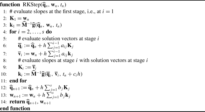

  

  Numerical algorithm for computing one step with an explicit RK method with $s$ stages. The symbol “#” represents start of comments

  Algorithm 3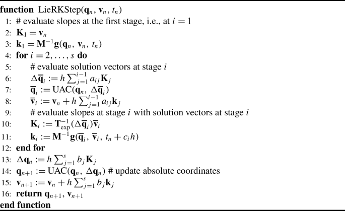

  

  Numerical algorithm for computing one step with an explicit RKMK method with $s$ stages. The symbol “#” represents start of comments

• 2. The kinematic equation $\dot{\widehat{\mathbf {q}}}$ in Eq. (32) must be replaced by the kinematic equation (25). This modification is shown in line 10 in Algorithm 3.

• 3. Instead of calculating the slopes with Eq. (32) (see lines 3 and 10 in Algorithm 2), Lie group time integration methods require the slopes to be calculated using the equilibrium conditions (23). This modification is shown in lines 3 and 11 in Algorithm 3.

3.2.1 Automatic step size control for RKMK methods

Advanced explicit time integration methods such as ODE23 [35] and DOPRI5 [36] include automatic step size control and are well established in MBD for solving Eq. (32). Variable step size implementations for solving Eq. (23) with RKMK methods have been discussed in a recent paper of Celledoni et al.; see [29]. In this paper, we follow a slightly different approach, which is summarized in Appendix B and [37].

3.3 Implicit time integration

In this section, we show how an MBS formalism that employs the generalized-$\alpha$ method [25, 26] for the time integration of the EOMs in parameterized form (12) has to be modified to obtain Lie group generalized-$\alpha$ [1]. In [26], a function AlphaStep has been introduced that solves the EOMs in parameterized form (12) at time $t_{{n+ 1}}$ using the generalized-$\alpha$ method. In the following, we show how AlphaStep can be modified to obtain Lie group generalized-$\alpha$.

The function AlphaStep (see Algorithm 4) represents a Newton method with unknowns $\widehat{\mathbf {q}}$ and $\boldsymbol{\lambda }$, and solves Eq. (12) at time $t_{{n+ 1}}$ and involves the parameters

$$ \beta ^{\prime }= \dfrac{1-\alpha _{m}}{h^{2} \beta (1-\alpha _{f})}, \quad \gamma ^{\prime }= \dfrac{\gamma}{h \beta}, $$

(33)

the residual vector

$$ \widehat{\mathbf{r}}(\widehat{\mathbf {q}}, \dot{\widehat{\mathbf {q}}}, \ddot{\widehat{\mathbf {q}}}, \boldsymbol{\lambda }, t) = \widehat{\mathbf{M}}( \widehat{\mathbf {q}})\ddot{\widehat{\mathbf {q}}}- \widehat{\mathbf{H}}^{T}(\widehat{\mathbf {q}})\left ( \widehat{\mathbf{g}}(\widehat{\mathbf {q}}, \dot{\widehat{\mathbf {q}}}, t) - \widehat{\mathbf{B}}^{T}( \widehat{\mathbf {q}}) \boldsymbol{\lambda }\right ) $$

(34)

and the iteration matrix⁸

$$ \widehat{\mathbf {S}}_{t}= \begin{bmatrix} \widehat{\mathbf{M}}(\widehat{\mathbf {q}})\beta ^{\prime }+ \widehat{\mathbf{C}}_{t}(\widehat{\mathbf {q}}, \dot{\widehat{\mathbf {q}}}, t)\gamma ^{\prime }+ \widehat{\mathbf{K}}_{t}(\widehat{\mathbf {q}}, \dot{\widehat{\mathbf {q}}}, \ddot{\widehat{\mathbf {q}}}, \boldsymbol{\lambda }, t) & & \widehat{\mathbf{H}}^{T}( \widehat{\mathbf {q}})\widehat{\mathbf{B}}^{T}(\widehat{\mathbf {q}}) \\ \widehat{\mathbf{H}}(\widehat{\mathbf {q}})\widehat{\mathbf{B}}( \widehat{\mathbf {q}}) & & \mathbf{0}\end{bmatrix} , $$

(35)

which is also denoted as Jacobian. The numerical parameters $\alpha _{m}$, $\alpha _{f}$, $\beta$ and $\gamma$ in Eqs. (33)–(35) can be selected by choosing the numerical damping $\rho _{\infty}\in [0,1]$ in order to have suitable accuracy and stability properties [26]. In Eq. (35), the tangent stiffness and damping matrices $\widehat{\mathbf{K}}_{t}$ and $\widehat{\mathbf{C}}_{t}$ are calculated by

$$\begin{aligned} \widehat {\mathbf {K}}_{t}(\widehat {\mathbf {q}}, \dot {\widehat {\mathbf {q}}}, \ddot {\widehat {\mathbf {q}}}, \boldsymbol {\lambda }, t) &= \dfrac{\partial \widehat {\mathbf {r}}(\mathbf{z}, \dot {\widehat {\mathbf {q}}}, \ddot {\widehat {\mathbf {q}}}, \boldsymbol {\lambda }, t)}{\partial \mathbf{z}} \bigg\vert _{\mathbf{z}=\widehat {\mathbf {q}}} \end{aligned}$$

(36)

$$\begin{aligned} &\approx - \dfrac{\partial \widehat{\mathbf {H}}^{T}(\mathbf{z}) \widehat {\mathbf {g}}(\mathbf{z}, \dot {\widehat {\mathbf {q}}}, t)}{\partial \mathbf{z}} \bigg\vert _{\mathbf{z}=\widehat {\mathbf {q}}}, \end{aligned}$$

(37)

$$\begin{aligned} \widehat {\mathbf {C}}_{t}(\widehat {\mathbf {q}}, \dot {\widehat {\mathbf {q}}}, t) &= - \dfrac{\partial \widehat{\mathbf {H}}^{T}(\widehat {\mathbf {q}})\widehat {\mathbf {g}}(\widehat {\mathbf {q}}, \mathbf{z} , t)}{\partial \mathbf{z}} \bigg\vert _{\mathbf{z}=\dot {\widehat {\mathbf {q}}}}, \end{aligned}$$

(38)

where we use Eq. (37) in our implementation. Note that in Algorithm 4, the auxiliary variable $\mathbf{a}$ is set to⁹$\mathbf{a}_{0}=\ddot{\widehat{\mathbf {q}}}_{0}$ for time $t=0$; see [26].

Algorithm 4

Numerical algorithm for computing a Newton update for generalized-$\alpha$ according to [26]

The modifications required to transform AlphaStep (Algorithm 4) into a Lie group method, i.e., SolveTimeStep [1], are illustrated in Algorithm 5 and are given in the subsequent listing.

• 1. The unknowns in the Newton method are now $\Delta \mathbf{q}$ and $\boldsymbol{\lambda }$; cf. Sect. 3.1.

• 2. The absolute coordinates $\mathbf{q}$ have to be determined via the LGT map (24). For this, the vector $\Delta \mathbf{q}$ must be calculated in addition to $\mathbf{q}$. This modification is shown in lines 5–6 and 14–15 in Algorithm 5. Note that the latter modification might be also achieved by (1) introducing an additional data coordinate $\hat{\mathbf {q}}_{n}$ that stores $\mathbf{q}_{n}$, i.e., $\hat{\mathbf {q}}_{n}= \mathbf{q}_{n}$, and (2) by setting $\mathbf{q}_{n}= \mathbf{0}$. The data coordinate $\hat{\mathbf {q}}_{n}$ may then be used instead of $\mathbf{q}_{n}$ to update the absolute coordinates in lines 6 and 15.

  Algorithm 5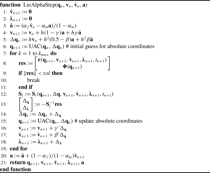

  

  Numerical algorithm computing a Newton update for Lie generalized-$\alpha$. The symbol “#” represents start of comments

• 3. The residual vector Eq. (34) has to be computed with the equilibrium conditions in Eq. (23), which now reads

  $$ \mathbf{r}(\mathbf{q}, \mathbf{v}, \dot{\mathbf {\mathbf {v}}}, \boldsymbol{\lambda }, t) = \mathbf{M}(\mathbf{q}) \dot{\mathbf {\mathbf {v}}}- \mathbf{g}(\mathbf{q},\mathbf{v}, t) + \mathbf{B}^{T}(\mathbf{q}) \boldsymbol{\lambda }. $$

  (39)

  This modification is shown in line 8 in Algorithm 5.

• 4. The iteration matrix Eq. (35) has to be computed differently. For Lie group generalized-$\alpha$, the iteration matrix is given by [1, 9, 23]

  $$ \begin{aligned} &\mathbf{S}_{t}(\mathbf{q}, \Delta \mathbf{q}, \mathbf{v}, \dot{\mathbf {\mathbf {v}}}, \boldsymbol{\lambda }, t) \\ &\quad = \begin{bmatrix} \mathbf{M}(\mathbf{q})\beta ^{\prime }+ \mathbf{C}_{t}( \mathbf{q}, \mathbf{v}, t)\gamma ^{\prime }+ \mathbf{K}_{t}(\mathbf{q}, \mathbf{v}, \dot{\mathbf {\mathbf {v}}}, \boldsymbol{\lambda }, t)\mathbf{T}_{\textrm{exp}}( \Delta \mathbf{q}) & & \mathbf{B}^{T}(\mathbf{q}) \\ \mathbf{B}(\mathbf{q})\mathbf{T}_{\textrm{exp}}(\Delta \mathbf{q}) & & \mathbf{0} \end{bmatrix}. \end{aligned} $$

  (40)

  This modification is shown in line 12 in Algorithm 5. In this paper, the tangent stiffness matrix¹⁰$\mathbf{K}_{t}$ reads

  $$\begin{aligned} \mathbf {K}_{t}(\mathbf {q}, \mathbf {\mathbf {v}}, \dot {\mathbf {\mathbf {v}}}, \boldsymbol {\lambda }, t) &= \dfrac{\partial \mathbf {r}(\mathrm{UAC}(\mathbf {q},\, \mathbf{z}), \mathbf {\mathbf {v}}, \dot {\mathbf {\mathbf {v}}}, \boldsymbol {\lambda }, t)}{\partial \mathbf{z}} \bigg\vert _{\mathbf{z}=\mathbf {0}} \end{aligned}$$

  (41)
  $$\begin{aligned} &\approx - \dfrac{\partial \mathbf {g}(\mathrm{UAC}(\mathbf {q},\, \mathbf{z}), \mathbf {\mathbf {v}}, t)}{\partial \mathbf{z}} \bigg\vert _{\mathbf{z}=\mathbf {0}}, \end{aligned}$$

  (42)

  where we use Eq. (42) in our implementation.¹¹ The damping matrix $\mathbf{C}_{t}$ in Eq. (40) reads

  $$ \mathbf{C}_{t}(\mathbf{q}, \mathbf{v}, t) = - \dfrac{\partial \mathbf{g}(\mathbf{q}, \mathbf{z}, t)}{\partial \mathbf{z}} \bigg\vert _{\mathbf{z}=\mathbf{v}}. $$

  (43)

  Practical experiments have shown that the tangent operator $\mathbf{T}_{\textrm{exp}}(\Delta \mathbf{q})=\mathbf{I}+ \mathcal{O}( \Vert \Delta \mathbf{q}\Vert )$ can be neglected in Eq. (40) for small time steps, which we do throughout this paper and will illustrate in the numerical examples in Sect. 4. Note however that neglecting the tangent operator in Eq. (40) may lead to stability problems but may prevent the destruction of sparsity structures of the system matrices in the simulation code.

Both iteration matrices Eq. (35) and Eq. (40) become severely ill conditioned for small time step sizes $h$ [9, 26]. To avoid this phenomenon, we use the scaling method proposed by Bottasso et al. in [38] in our implementation. The scaling of the iteration matrix for the generalized-$\alpha$ method and its Lie group counterpart are discussed, for example, in [9, 26, 39].

3.4 Modified Newton method

Evaluating the iteration matrix (35) respectively (40) might be time-consuming in the full Newton method, where the Jacobian is computed in each Newton iteration. Therefore, to increase computational performance, we compute an update and factorization of the iteration matrix in the so-called “modified Newton method” only if needed. Therein, the iteration matrix is computed at the beginning of the simulation and updated during the iteration process only if either a predefined maximum number of Newton iterations is reached or the error in each Newton iteration could not be reduced by a predefined tolerance [37, 40].

3.5 Effects of round-off errors in $\mathbf{T}_{\textrm{exp}}$ and $\mathbf{T}^{-1}_{\textrm{exp}}$

In our numerical experiments, we observed effects of round-off errors in the evaluation of the tangent operator $\mathbf{T}_{\textrm{exp}}$ respectively its inverse near $\Vert{\Delta \mathbf{q}} \Vert =\mathbf{0}$. The effects of round-off errors when evaluating tangent operators have also been reported in [41] and are termed there as a loss of significance. To obtain accurate and precise results, we use Taylor approximations for those terms that cause the loss of significance. The approximation strategy is presented in Appendix A.2.

4 Numerical examples

In this section, we compare the classical formulations 1 and 2 with an LGIM in terms of accuracy and computational performance using five typical rigid body systems. In the LGIM, the rotation vector is used to represent the orientation of a rigid body; see Sect. 3.1. In both classical formulations, Cardan/Tait–Bryan angles (123-Euler angles, cf. [37, 42]) are used as rotation parameters. Euler parameters are used only in the classical formulation 2 in combination with implicit integration and by imposing the Euler parameter unit length condition as an additional constraint equation on position level; cf. [37]. Both the LGIM and the classical formulation 1 are used in combination with explicit and implicit time integration methods. In all numerical examples, the following abbreviations are used:

• “Rxyz” means Cardan/Tait–Bryan angles (classical formulation 2),

• “RV” means rotation vector (LGIM),

• “EP” means Euler parameter (classical formulation 2).

The abbreviations used in the following for the explicit RK and RKMK methods, such as RK44, follow the designations used in [34].

All rigid body systems considered are set up and simulated in Exudyn¹² [37, 43] using version 1.4.5.dev1 and Python 3.7 64bit. Note that the LGIM has been implemented in C++ focusing on efficiency. All simulations have been performed in Windows 10 on an Intel Core i7-6600U 2.60 GHz processor. The absolute and relative error tolerances $a_{tol}$ and $r_{tol}$ for automatic step size control have been chosen in each numerical example as $r_{tol}= 10^{-2} / (t_{End}/h)^{p}$ and $a_{tol} = r_{tol} \times 10^{-2}$, where $t_{End}$ represents the simulation period and $p$ the order of the integration method. The spectral radius is set to $\rho _{\infty}=0.9$ for generalized-$\alpha$ and Lie group generalized-$\alpha$ for all examples.

4.1 Heavy top

The first rigid body system we consider is the benchmark example “heavy top”; see Fig. 1. Two simulation cases are considered, which are described in the following two sections. In both cases, we simulate the motion of the heavy top over a period of $t=1\text{ s}$. Model parameters and initial conditions are summarized in Table 3.

Fig. 1

Benchmark problem Heavy top; see, e.g., Ref. [1]

Table 3 Model parameters and initial conditions of the heavy top

4.1.1 Heavy top without kinematic constraints

In the first investigations, we consider the heavy top without kinematic constraints according to Refs. [1, 3, 10, 11, 29].

In Fig. 2, the time histories of the heavy top’s center of mass (COM) position coordinates (left plot) and translational velocity coordinates (right plot) computed with Lie group generalized-$\alpha$ are compared with reference solutions computed with the multibody simulation software RecurDyn.¹³ As can be seen in Fig. 2, the time histories obtained with Lie group generalized-$\alpha$ visually match the reference solutions. The absolute deviation of the heavy top’s position and velocity coordinates at $t=1\text{ s}$ is approximately $1.0\times 10^{-5}\text{ m}$ respectively $1.0\times 10^{-5}\text{ m}/\text{s}$. Similar results have been obtained for explicit Lie group time integration.

Fig. 2

Time histories of the heavy top’s center of mass position (left plot) and translational velocity coordinates (right plot) expressed in the global frame. Reference solutions were computed over a simulation time of $t = 1\text{ s}$ with a time step size of $h=2.5\times 10^{-5}\text{ s}$ using RecurDyn. The heavy top’s center of mass position and translational velocity coordinates obtained with Euler parameters and generalized-$\alpha$ are computed for comparison purposes over $t = 0.8\text{ s}$

In Fig. 3, the convergence in the norm of the COM position error $\Vert \mathbf{x}_{Ref} - \mathbf{x}\Vert$ is illustrated for explicit (left plot) and implicit time integration (right plot). The fixed time step sizes used in the convergence analysis are calculated by $h_{n} = (1.0\times 10^{-4}\times 2^{(1-n)})_{n=1,2,\ldots,8}$. Convergence is investigated at $t = 1\text{ s}$. The reference solution for the convergence analysis $\mathbf{x}_{Ref}$ was computed using the LGIM and an explicit RK method with order six using a time step size of $h_{Ref}=3.90625\times 10^{-6}\text{ s}$. As can be seen in Fig. 3, in case of explicit time integration, LGIM outperforms the conventional approach in terms of accuracy. In contrast, the conventional Euler parameter approach is more accurate than Lie group time integration for implicit integration; see Fig. 3 (right plot).

Fig. 3

Convergence in the norm of the maximum error of the heavy top without kinematic constraints COM position for different rotation parameters and time integration methods. Left plot, explicit integration; right plot, implicit integration (generalized-$\alpha$)

At this point, we conclude that Euler parameters only give nonlinearities with low-order polynomials, e.g., in the rotation matrix, which seem to be more suitable for the second-order time integrator than the Lie group method.

In Table 4 the average number of Newton iterations per time step needed for the simulation of the heavy top is given. As can be seen in Table 4, the average number of Newton iterations per time step is lower for Lie group time integration as compared to the conventional approaches, which is due to the reduced nonlinearities in the EOMs for Lie group methods.

Table 4 Average number of Newton iterations per time step needed in generalized-$\alpha$ for different rotation parameters: benchmark heavy top without kinematic constraints

The CPU time needed for simulation is shown in Fig. 4 for explicit (left plot) and implicit integration (right plot). As can be seen in Fig. 4, the CPU time is on average shorter in the case of Lie group time integration, both explicit and implicit, than in the conventional approaches. In the case of implicit integration, the latter observation is in line with our expectations, since the lower number of Newton iterations required by the LGIM compared to the two conventional approaches should also be reflected in the CPU time. In contrast to the expectation, in case of explicit integration, the additional computational effort required by the LGIM¹⁴ compared to the conventional approach (compare Algorithm 2 with Algorithm 3) does not seem to have a big effect on the CPU time. The shorter CPU time of the LGIM stems from the fact that the mass matrix is constant and therefore does not need to be recomputed and factorized in each time step. However, this is not the case for the conventional Rxyz formulation. Similar behavior is observed in all other numerical examples considered, as will be shown in the remainder of this paper.

Fig. 4

CPU time of “heavy top without kinematic constraints” for different rotation parameters and time integration methods. Left plot, explicit integration; right plot, implicit integration (generalized-$\alpha$)

Finally, Fig. 5 shows the work–precision diagrams for explicit and implicit integration. As illustrated in Fig. 5, the CPU time required to achieve, for example, an accuracy of $1.0 \times 10^{-6}$ with Cardan/Tait–Bryan angles and RK44 is about 40 times higher than with the LGIM. In contrast, the conventional Euler parameter approach requires only about a quarter of the CPU time needed by the LGIM to achieve an accuracy of $1.0 \times 10^{-4}$ in case of implicit integration.

Fig. 5

Work–precision diagrams for explicit and implicit time integration methods for the example “heavy top without kinematic constraints.” Left plot, explicit integration; right plot, implicit integration (generalized-$\alpha$)

4.1.2 Heavy top with kinematic constraints

In the second investigations, we consider the heavy top with kinematic constraints according to Refs. [1, 2, 9, 17, 22, 23, 28–30].

In Fig. 6, the convergence in the norm of the heavy top’s COM position error $\Vert \mathbf{x}_{Ref} - \mathbf{x}\Vert$ is illustrated for implicit time integration and different types of Newton methods; cf. Sect. 3.4. The time step sizes used in the convergence analysis are calculated again by $h_{n} = (1.0\times 10^{-4}\times 2^{(1-n)})_{n=1,2,\ldots,8}$ and convergence is investigated at $t = 1\text{ s}$. The reference solution $\mathbf{x}_{Ref}$ has been computed with the conventional EP approach and generalized-$\alpha$ using a time step size of $h_{Ref}=1\times 10^{-7}\text{ s}$.

Fig. 6

Convergence in the norm of the maximum error of the heavy top with kinematic constraints COM position for different rotation parameters and generalized-$\alpha$ using different Newton methods. Left plot, full Newton; right plot, modified Newton

As can be seen in Fig. 6, the conventional EP approach is again more accurate than Lie group time integration both for full Newton and modified Newton. However, the LGIM can simulate the heavy top even at the largest considered time step sizes as compared to both classical approaches.

As expected, the number of Newton iterations for “modified Newton” is larger compared to “full Newton”; see Fig. 7. Figure 7 also shows that the number of Newton iterations is lower for Lie group time integration than in the conventional approaches, which results in a shorter CPU time as shown in Fig. 8. Finally, Table 5 shows the average number of Newton iterations required per time step when the tangent operator $\mathbf{T}_{\textrm{exp}}$ is considered or neglected in Eq. (40). As can be seen from Table 5, neglecting $\mathbf{T}_{\textrm{exp}}$ in the iteration matrix (40) leads to a larger number of Newton iterations per time step at time step sizes $h \geq 4.0\times 10^{-5}\text{ s}$, which corresponds at time $t=1\text{ s}$ to an incremental rotation of $\Vert \Delta \boldsymbol{\boldsymbol {\psi }}\Vert \approx \Vert h\,{ \boldsymbol{\omega }}\Vert \approx 6.0 \times 10^{-3}\text{ rad}$. However, for time step sizes $h < 4.0\times 10^{-5}\text{ s}$, neglecting $\mathbf{T}_{\textrm{exp}}$ in Eq. (40) no longer affects the number of Newton iterations needed per time step. As can be seen in Table 5, including $\mathbf{T}_{\textrm{exp}}$ in Eq. (40) within the modified Newton method has hardly any effect on the required Newton iterations per time step; cf. Fig. 7. We observed similar results in all other numerical examples.

Fig. 7

Number of Newton iterations (generalised-$\alpha$) required in the “heavy top with kinematic constraints” example for different Newton methods and rotation parameters. Left plot, full Newton; right plot, modified Newton. For the LGIM (RV), $\mathbf{T}_{\textrm{exp}}$ is included in Eq. (40)

Fig. 8

CPU time (generalised-$\alpha$) required in the “heavy top with kinematic constraints” example for different Newton methods and rotation parameters. Left plot, full Newton; right plot, modified Newton

Table 5 Average number of Newton iterations per time step needed in Lie group generalized-$\alpha$ when the tangent operator $\mathbf{T}_{\textrm{exp}}$ is considered or neglected in Eq. (40): benchmark heavy top with kinematic constraints

4.2 High-speed rotor with flexible supports

We investigate the performance of Lie group time integration methods compared to the conventional approaches considered using a flexibly supported high-speed rotor; see Fig. 9. The model parameters are given in Table 6. The rotor is subjected to a torque of

$$ \mathbf{t}= \begin{bmatrix} 0 & & 0 & & (\frac{L}{2} - L_{L})mg \end{bmatrix} ^{T}. $$

(44)

All simulations are performed over a period of $t=4\text{ s}$.

Fig. 9

Schematic representation of high-speed rotor with flexible supports

Table 6 Model parameters of “high-speed rotor with flexible supports”

In Fig. 10, the trajectory of point $\mathbf{p}_{1}=[-L_{L},\,0.0,\,0.0]$ in the $y$-$z$-plane (left plot) and the time history of its coordinates (right plot) are shown. Figure 10 was obtained using the LGIM in combination with an explicit RK method with order six (RK67) and a time step size of $h=1.0 \times 10^{-5}\text{ s}$. As can be seen in the left plot of Fig. 10, the rotor performs a precession motion, whereby the precession period is about 2.5 s (cf. Fig. 10, right plot), which corresponds to a precession frequency of 0.4 Hz.

Fig. 10

Left: Trajectory of point $\mathbf{p}_{1}$ on the rotor located at the position of the left support. Right: Time history of the components of the angular velocity vector represented in the local frame. Left plot, tilting motion of the rotor; right plot, position coordinates of point $\mathbf{p}_{1}$

In Fig. 11, the convergence in the norm of the position error $\Vert \mathbf{p}_{Ref} - \mathbf{p}\Vert$ of point $\mathbf{p}_{1}$ on the rotor is illustrated for explicit time integration (left plot) and for implicit time integration (right plot). The fixed time step sizes used in the convergence analysis are calculated by $h_{n} = (1.0\times 10^{-4}\times 2^{(1-n)})_{n=1,2,\ldots,8}$. Convergence is investigated at $t = 4\text{ s}$. The reference solution $\mathbf{p}_{Ref}$ for the convergence analysis was computed using the conventional approach Rxyz and RK67 using a time step size of $h_{Ref}=1.0\times 10^{-6}\text{ s}$. As can be seen in Fig. 11, Lie group time integration outperforms the conventional approach in terms of accuracy in case of explicit time integration. In contrast, the conventional EP approach is again more accurate than the LGIM in case of implicit integration; see Fig. 11 (right plot). However, in contrast to the conventional EP approach, both the LGIM and the conventional Rxyz approach can simulate the rotor even at the largest considered time step sizes.

Fig. 11

Convergence in the norm of the maximum error of point $\mathbf{p}_{1}$ on the rotor located at the position of the left support for different rotation parameters and time integration methods. Left plot, explicit integration; right plot, implicit integration (generalized-$\alpha$)

In Table 7 the average number of Newton iterations per time step needed for the simulation of the rotor is given. As can be seen in Table 7, the average number of Newton iterations per time step is smaller for LGIM as compared to the conventional approaches.

Table 7 Average number of Newton iterations per time step needed in generalized-$\alpha$ for different rotation parameters: high-speed rotor with flexible supports

The CPU time needed for simulation of the high-speed rotor is shown in Fig. 12 for explicit integration (right plot) and for implicit integration (left plot). As with the previous numerical examples, the CPU time is in the case of the LGIM on average equal or even smaller as compared to the conventional approaches, both for explicit and implicit integration.

Fig. 12

CPU time of “high-speed rotor with flexible supports” for different rotation parameters and time integration methods. Left plot, explicit integration; right plot, implicit integration (generalized-$\alpha$)

Finally, Fig. 13 shows the work–precision diagrams for explicit (left plot) and implicit (right plot) integration. As illustrated in Fig. 13, the CPU time required to achieve, for example, an accuracy of $1.0 \times 10^{-9}$ with Cardan/Tait–Bryan angles and DOPRI5 or RK67 is about 10 times higher than with the LGIM. Figure 13 also shows that the LGIM achieves in this example in case of implicit integration a higher performance than the conventional Rxyz approach and a similar performance to the conventional Euler parameter approach.

Fig. 13

Work–precision diagrams for explicit and implicit time integration methods for the example “high-speed rotor with flexible supports.” Left plot, explicit integration; right plot, implicit integration (generalized-$\alpha$)

4.3 Spatial rigid Slider–Crank mechanism

In the next investigations, we compare the accuracy and computational performance of LGIM with both conventional approaches using the slider–crank mechanism shown in Fig. 14. The spatial rigid slider–crank mechanism is an MBD benchmark problem taken from the library of computational benchmark problems by IFToMM [44] and is illustrated in Fig. 14.

Fig. 14

Spatial rigid slider–crank mechanism [45]

The spatial slider–crank mechanism consists of four rigid bodies: a slider, a crank, a connecting rod and the ground. The crank (AB) has a length of 0.08 m and is connected to the ground by a revolute joint at point A. The crank is driven from initial crank angle $\theta =0\text{ rad}$ with an initial angular velocity of 6 rad/s. The connecting rod has a length of 0.3 m and is connected to the crank by a spherical joint at point B and to the slider by a universal joint at point C. The slider is connected to the ground by a prismatic joint at point D with sliding displacement $s$. All links are subjected to gravity of magnitude 9.81 m/s² in the negative $z$-direction. Studying the dynamic response of the slider–crank mechanism under the gravitational force is the main objective of this benchmark problem. The model parameters and initial conditions are summarized¹⁵ in Table 8.

Table 8 Model parameters and initial conditions of the slider–crank mechanism. All quantities are expressed with respect to the center of mass of the respective rigid body

In Fig. 15, the time histories of the slider–crank’s slider position coordinate $s$ (Fig. 15a) and crank angle $\theta$ (Fig. 15b) are compared with reference solutions provided by IFToMM [44]. Figure 15 was obtained using the conventional Rxyz approach and generalized-$\alpha$ with time step size $h=1.0 \times 10^{-5}\text{ s}$. As can be seen in Fig. 15, the time histories obtained with generalized-$\alpha$ and Euler parameters visually match the reference solution. The absolute deviation of the slider–crank’s slider position $s$ at $t=5\text{ s}$ is approximately $8.6\times 10^{-3}\text{ m}$. The difference between our solution and the solution provided by IFToMM is due to the fact that different time integration methods were used; see [44].

Fig. 15

Time histories of the slider–crank’s slider position and crank angle. The reference solution ($s_{Masarati}$) was taken from the library of computational benchmark problems IFToMM [44]

In Fig. 16, the convergence in the norm of the slider position error is shown for generalized-$\alpha$ and different formulations for decreasing values of the time step $h_{n} = (4.0\times 10^{-3}\times 2^{(1-n)})_{n=1,2,\ldots,13}$. Convergence is investigated at $t = 5\text{ s}$. The reference solution $s_{Ref}$ for the convergence analysis was computed using the conventional approach Rxyz and generalized-$\alpha$ using a time step size of $h_{Ref}=1.0\times 10^{-6}\text{ s}$. As can be seen in Fig. 16, the conventional approaches are more accurate than the LGIM for time step sizes $h > 1.0\times 10^{-4}\text{ s}$. For time step sizes $h \leq 1.0\times 10^{-5}\text{ s}$, the LGIM appears to be partially slightly more accurate than both conventional approaches.

Fig. 16

Convergence in the norm of the maximum error of the slider–crank’s slider position for different rotation parameters and generalized-$\alpha$

In Fig. 17 (left plot) the average number of Newton iterations per time step needed for the simulation of the slider–crank mechanism is illustrated. As can be seen in Fig. 17, the average number of Newton iterations per time step is lower for the conventional approach Rxyz compared to the LGIM and the Euler parameter approach. The CPU time needed for simulation of the slider–crank mechanism is shown in Fig. 17 (right plot). As expected from the lower number of Newton iterations required in the Rxyz formulation compared to the Lie group and Euler parameter formulations, the CPU time of the Rxyz formulation turns out to be on average the lowest.

Fig. 17

Average number of Newton iterations per time step and CPU time of the slider–crank simulation for different rotation parameters and time implicit integration methods. Left plot, Newton iterations; right plot, CPU time

4.4 Puma 560 robot

Finally, we consider the Puma 560 robot (Programmable Universal Manipulator for Assembly), which is illustrated schematically in Fig. 18a. The Puma robot consists of six rigid bodies [46] and its kinematic chain with six revolute joints is illustrated in Fig. 18b. In total, the Puma robot has six degrees of freedom. The robot performs a point-to-point motion using constant joint acceleration profiles, whereby all links are subjected to gravity of magnitude 9.81 m/s² in the negative $z$-direction. The constant joint acceleration profiles are give in Table 9. The point-to-point motion starts with initial joint angles $\boldsymbol{\varphi}^{init}$ and aims to reach the goal configuration defined by the joint angles $\boldsymbol{\varphi}^{Goal}$:

$$ \boldsymbol{\varphi}^{init} = \begin{bmatrix} \varphi _{1} \\ \varphi _{2} \\ \varphi _{3} \\ \varphi _{4} \\ \varphi _{5} \\ \varphi _{6} \end{bmatrix} = \begin{bmatrix} 0.0^{\circ } \\ 22.5^{\circ} \\ 90.0^{\circ} \\ 0.0^{\circ} \\ 22.5^{\circ} \\ 0.0^{\circ }\end{bmatrix} , \quad \boldsymbol{\varphi}^{Goal} = \begin{bmatrix} \varphi _{1}^{Goal} \\ \varphi _{2}^{Goal} \\ \varphi _{3}^{Goal} \\ \varphi _{4}^{Goal} \\ \varphi _{5}^{Goal} \\ \varphi _{6}^{Goal} \end{bmatrix} = \begin{bmatrix} -120.0^{\circ } \\ 60.0^{\circ } \\ -200.0^{\circ } \\ 90.0^{\circ } \\ 90.0^{\circ } \\ 45.0^{\circ }\end{bmatrix} . $$

(45)

In Fig. 19, the time histories of the robot’s joint angles are shown, which where computed using the conventional Euler parameter approach and a time step size of $h =1.0\times 10^{-4}\text{ s}$. The Puma P560 robot has been well studied and its parameters are very well known [46]. The standard Denavit–Hartenberg parameters, as well as the physical parameters of the Puma robot, can be found in many textbooks on robotics, such as [46, 47] for example, and are omitted here due to space reasons. In each joint, a PD controller, which is implemented in the simulation model as a spring–damper element with control parameters specified in Table 10, ensures that the prescribed trajectory is followed with minimal error. In the following, we compare the accuracy and computational performance of the LGIM and both conventional approaches with a minimal coordinate formulation [48], which is abbreviated as “Min. Coord.” hereafter.

Fig. 18

Schematic representation of the Puma P560 manipulator and its kinematic chain

Fig. 19

Joint angles

Table 9 Values of constant angular acceleration profiles used for the point-to-point motion

Table 10 PD controller parameters of the Puma P560 manipulator

In Fig. 20, the convergence in the norm of the robot’s joint angles is illustrated. The time step sizes used in the convergence analysis are calculated by $h_{n} = (1.0\times 10^{-1}\times 2^{(1-n)})_{n=1,2,\ldots,11}$. Convergence is investigated at $t = 1\text{ s}$ and the reference solution $\boldsymbol{\varphi}_{Ref}$ was computed by employing the minimal coordinate formulation and generalized-$\alpha$ using a time step size of $h_{Ref}=1.0\times 10^{-6}\text{ s}$. As can be seen in Fig. 20, the minimal coordinate formulation is the most accurate for all considered time step sizes. The classical Euler parameter approach and the LGIM exhibit for time step sizes $h > 1.56\times 10^{-2}\text{ s}$ virtually the same accuracy, while the classical Euler parameter approach is more accurate at smaller time step sizes. The conventional Rxyz approach is the least accurate. Moreover, both the LGIM and the conventional Euler parameter approach can simulate the Puma at almost the largest considered time step sizes, in contrast to the conventional Rxyz approach. However, the minimal coordinate formulation outperforms both the LGIM and the conventional approaches in this regard. At this point we would like to note that the relative tolerance in “full Newton” had to be increased to $1.0\times 10^{-5}$ in order for Newton’s method to converge in the case of the LGIM.

Fig. 20

Convergence in the norm of the maximum error of the robot’s joint angles for different formulations and generalized-$\alpha$

In Fig. 21, the average number of Newton iterations per time step (left plot) and the CPU time (right plot) needed for simulation of the Puma robot are shown. As can be seen in Fig. 21, the LGIM achieves the lowest number of Newton iterations per time step for time step sizes $h \leq 1.0\times 10^{-3}\text{ s}$, while the LGIM requires also the most Newton iterations per time step for time step sizes $h > 3.12\times 10^{-2}\text{ s}$. Similar to the other numerical examples considered, the classical Rxyz approach requires on average fewer Newton iterations per time step than the conventional Euler parameter approach. These observations are reflected in the CPU time required; see Fig. 21 (left plot). It is worth noting that the minimal coordinate formulation achieves the lowest CPU time, which is due to the fact that only six EOMs need to be treated in the minimal coordinate formulation, while in the LGIM and both conventional approaches $6\times (3+l)$ equilibrium equations (1) and $6 \times 5$ holonomic constraints (3) need to be treated.

Fig. 21

Average number of Newton iterations per time step and CPU time required by the generalized-$\alpha$ method in the example “serial 6R robot” for different rotation parameters. Left plot, Newton iterations (full Newton); right plot, CPU time

5 Conclusion

The accuracy and computational performance of explicit and implicit LGIMs have been compared with classical Euler angle and Euler parameter-based formulations using a set of rigid body systems. It has been found that explicit LGIMs outperform classical parameterization-based formulations in terms of accuracy, while the computational efficiency is almost the same. Especially for systems with high rotational speeds, explicit LGIMs turn out to be more accurate than the classical formulations. In contrast, in the case of implicit integration, the classical Euler parameter-based formulation outperforms both the classical Euler angle formulation and the LGIM in terms of accuracy. The LGIM appears to be computationally more efficient, as the number of Newton iterations required in each time step is lower compared to the classical formulations. The number of Newton iterations may be further reduced in case of changing from the $\mathbb{R}^{3}\times SO(3)$ formulation to the $SE(3)$ formulation, which reduces nonlinearities in equations for one integration step. Furthermore, it has been illustrated how LGIMs can be implemented into an MBS formalism that is based on absolute coordinates. The implementation is shown for formalisms that employ explicit RK methods and the implicit generalized-$\alpha$ method. It turns out that LGIMs can be implemented at almost no extra cost, i.e., it takes only a few changes in the classical integration algorithms to convert them into LGIMs. The straightforward transition from classical integration methods to LGIMs is facilitated by the fact that LGIMs readily allow three rotation parameters to be used for modeling MBSs, which makes the dimension of the residual and the iteration matrix coincide with that of the absolute coordinates and thus existing data structures might be used. Up to now, we restricted our investigations to the $\mathbb{R}^{3}\times SO(3)$ formulation. Future work will address the evaluation of the $SE(3)$ formulation in terms of accuracy and computational performance compared to classical formulations using a set of rigid and flexible MBSs.

Appendices

Appendix A: Implementation details

1.1 A.1 Tangent operators

The tangent operator $\mathbf{T}_{\textrm{exp}}\in \mathbb{R}^{6\times 6}$ on $\mathbb{R}^{3}\times SO(3)$ and its inverse $\mathbf{T}^{-1}_{\textrm{exp}}\in \mathbb{R}^{6\times 6}$ are given by [3, 49]

$$ \mathbf{T}_{\textrm{exp}}(\Delta \mathbf{q}) = \begin{bmatrix} \mathbf{I}& \mathbf{0} \\ \mathbf{0}& \mathbf{T}_{\textrm{exp}_{SO(3)}}(\Delta \boldsymbol{\boldsymbol {\psi }}) \end{bmatrix} , \quad \mathbf{T}^{-1}_{\textrm{exp}}(\Delta \mathbf{q}) = \begin{bmatrix} \mathbf{I}& \mathbf{0} \\ \mathbf{0}& \mathbf{T}^{-1}_{\textrm{exp}_{SO(3)}}(\Delta \boldsymbol{\boldsymbol {\psi }}) \end{bmatrix} . $$

(A1)

In Eq. (A1), the matrices $\mathbf{T}_{\textrm{exp}_{SO(3)}}\in \mathbb{R}^{3\times 3}$ and $\mathbf{T}^{-1}_{\textrm{exp}_{SO(3)}}\in \mathbb{R}^{3\times 3}$ are the tangent operators on $SO(3)$ and read [2, 41]

$$\begin{aligned} \mathbf {T}_{\textrm {exp}_{SO(3)}}(\Delta \boldsymbol {\boldsymbol {\psi }}) &= \textstyle\begin{cases} \mathbf {I}& \text{if }\Vert {\Delta \boldsymbol {\boldsymbol {\psi }}} \Vert =0, \\ \mathbf {I}+ f_{1}(\Vert {\Delta \boldsymbol {\boldsymbol {\psi }}} \Vert )\widetilde {\Delta \boldsymbol {\psi }}+ f_{2}( \Vert {\Delta \boldsymbol {\boldsymbol {\psi }}} \Vert )\widetilde {\Delta \boldsymbol {\psi }}^{2} & \text{else}, \end{cases}\displaystyle \end{aligned}$$

(A2)

$$\begin{aligned} \mathbf {T}^{-1}_{\textrm {exp}_{SO(3)}}(\Delta \boldsymbol {\boldsymbol {\psi }}) &= \textstyle\begin{cases} \mathbf {I}& \text{if }\Vert {\Delta \boldsymbol {\boldsymbol {\psi }}} \Vert =0, \\ \mathbf {I}+ \dfrac{1}{2}\widetilde {\Delta \boldsymbol {\psi }}+ f_{3}(\Vert {\Delta \boldsymbol {\boldsymbol {\psi }}} \Vert ) \widetilde {\Delta \boldsymbol {\psi }}^{2} & \text{else}, \end{cases}\displaystyle \end{aligned}$$

(A3)

where

$$\begin{aligned} f_{1}(\Vert {\Delta \boldsymbol {\boldsymbol {\psi }}} \Vert ) &= \textstyle\begin{cases} \dfrac{\cos \Vert {\Delta \boldsymbol {\boldsymbol {\psi }}} \Vert - 1}{\Vert {\Delta \boldsymbol {\boldsymbol {\psi }}} \Vert ^{2}} & \text{if } \Vert {\Delta \boldsymbol {\boldsymbol {\psi }}} \Vert >0, \\ -\dfrac{1}{2} & \text{if }\Vert {\Delta \boldsymbol {\boldsymbol {\psi }}} \Vert =0, \end{cases}\displaystyle \end{aligned}$$

(A4)

$$\begin{aligned} f_{2}(\Vert {\Delta \boldsymbol {\boldsymbol {\psi }}} \Vert ) &= \textstyle\begin{cases} \dfrac{\Vert {\Delta \boldsymbol {\boldsymbol {\psi }}} \Vert - \sin \Vert {\Delta \boldsymbol {\boldsymbol {\psi }}} \Vert }{\Vert {\Delta \boldsymbol {\boldsymbol {\psi }}} \Vert ^{3}} & \text{if }\Vert {\Delta \boldsymbol {\boldsymbol {\psi }}} \Vert >0, \\ \dfrac{1}{6} & \text{if }\Vert {\Delta \boldsymbol {\boldsymbol {\psi }}} \Vert =0, \end{cases}\displaystyle \end{aligned}$$

(A5)

$$\begin{aligned} f_{3}(\Vert {\Delta \boldsymbol {\boldsymbol {\psi }}} \Vert ) &= \textstyle\begin{cases} \dfrac{1-\frac{\Vert {\Delta \boldsymbol {\boldsymbol {\psi }}} \Vert }{2}\cot \frac{\Vert {\Delta \boldsymbol {\boldsymbol {\psi }}} \Vert }{2}}{\Vert {\Delta \boldsymbol {\boldsymbol {\psi }}} \Vert ^{2}} & \text{if }\Vert {\Delta \boldsymbol {\boldsymbol {\psi }}} \Vert >0, \\ \dfrac{1}{12} & \text{if }\Vert {\Delta \boldsymbol {\boldsymbol {\psi }}} \Vert =0. \end{cases}\displaystyle \end{aligned}$$

(A6)

1.2 A.2 Handling loss of significance in $\mathbf{T}_{\textrm{exp}}$ and $\mathbf{T}^{-1}_{\textrm{exp}}$

There is a loss of significance when Eqs. (A4)–(A6) are evaluated near $\Vert{\Delta \boldsymbol{\boldsymbol {\psi }}} \Vert =0$ on a computer [41]. In order to obtain accurate and precise results from Eqs. (A4)–(A6) for all reasonable values of $\Vert{\Delta \boldsymbol{\boldsymbol {\psi }}} \Vert$, we approximate Eqs. (A4)–(A6) by Taylor polynomials. We choose the intervals where Eqs. (A4)–(A6) are evaluated by its Taylor approximation as proposed in [41]. The improved versions of Eqs. (A4)–(A6) read

$$\begin{aligned} f_{1}(\Vert {\Delta \boldsymbol {\boldsymbol {\psi }}} \Vert ) &= \textstyle\begin{cases} \dfrac{\cos \Vert {\Delta \boldsymbol {\boldsymbol {\psi }}} \Vert - 1}{\Vert {\Delta \boldsymbol {\boldsymbol {\psi }}} \Vert ^{2}} & \text{if } \Vert {\Delta \boldsymbol {\boldsymbol {\psi }}} \Vert \geq 1 \times 10^{-2}, \\ -\dfrac{1}{2} + \dfrac{\Vert {\Delta \boldsymbol {\boldsymbol {\psi }}} \Vert ^{2}}{24} - \dfrac{\Vert {\Delta \boldsymbol {\boldsymbol {\psi }}} \Vert ^{4}}{720} & \text{if } 0 \leq \Vert {\Delta \boldsymbol {\boldsymbol {\psi }}} \Vert < 1 \times 10^{-2}, \end{cases}\displaystyle \end{aligned}$$

(A7)

$$\begin{aligned} f_{2}(\Vert {\Delta \boldsymbol {\boldsymbol {\psi }}} \Vert ) &= \textstyle\begin{cases} \dfrac{\Vert {\Delta \boldsymbol {\boldsymbol {\psi }}} \Vert - \sin \Vert {\Delta \boldsymbol {\boldsymbol {\psi }}} \Vert }{\Vert {\Delta \boldsymbol {\boldsymbol {\psi }}} \Vert ^{3}} & \text{if }\Vert {\Delta \boldsymbol {\boldsymbol {\psi }}} \Vert \geq 1 \times 10^{-4}, \\ \dfrac{1}{6} - \dfrac{\Vert {\Delta \boldsymbol {\boldsymbol {\psi }}} \Vert ^{2}}{120} + \dfrac{\Vert {\Delta \boldsymbol {\boldsymbol {\psi }}} \Vert ^{4}}{5040} & \text{if } 0 \leq \Vert {\Delta \boldsymbol {\boldsymbol {\psi }}} \Vert < 1 \times 10^{-4}, \end{cases}\displaystyle \end{aligned}$$

(A8)

$$\begin{aligned} f_{3}(\Vert {\Delta \boldsymbol {\boldsymbol {\psi }}} \Vert ) &= \textstyle\begin{cases} \dfrac{1-\frac{\Vert {\Delta \boldsymbol {\boldsymbol {\psi }}} \Vert }{2}\cot \frac{\Vert {\Delta \boldsymbol {\boldsymbol {\psi }}} \Vert }{2}}{\Vert {\Delta \boldsymbol {\boldsymbol {\psi }}} \Vert ^{2}} & \text{if }\Vert {\Delta \boldsymbol {\boldsymbol {\psi }}} \Vert \geq 1 \times 10^{-2}, \\ \dfrac{1}{12} + \dfrac{\Vert {\Delta \boldsymbol {\boldsymbol {\psi }}} \Vert ^{2}}{720} + \dfrac{\Vert {\Delta \boldsymbol {\boldsymbol {\psi }}} \Vert ^{4}}{30240} & \text{if } 0 \leq \Vert {\Delta \boldsymbol {\boldsymbol {\psi }}} \Vert < 1 \times 10^{-2}, \end{cases}\displaystyle \end{aligned}$$

(A9)

which give an absolute error in the Taylor approximation of about $1 \times 10^{-16}$ and a relative error in the actual function of about $1 \times 10^{-10}$.

1.3 A.3 Composition operation for rotation vectors

We write the composition operation ⋄ for two rotation vectors $\boldsymbol{\psi }_{0}$ and $\Delta \boldsymbol{\boldsymbol {\psi }}$ with $\boldsymbol{\psi }$ being the resultant rotation vector as

$$ \boldsymbol{\psi }= \boldsymbol{\psi }_{0} \diamond \Delta \boldsymbol{\boldsymbol {\psi }}= \dfrac{\nu _{0}\,\boldsymbol{\eta }+ \eta _{0}\,\boldsymbol{\nu }+ \boldsymbol{\nu }\times \boldsymbol{\eta }}{2\,\mathrm{sinc}\,\varphi }, $$

(A10)

where

$${\eta }_0=cos\frac{\parallel {\mathit{\psi }}_0\parallel }{2},\mathit{\eta }=\frac{{\mathit{\psi }}_0}{2}\mathrm{sinc}\frac{\parallel {\mathit{\psi }}_0\parallel }{2},$$

(A11)

$${\nu }_0=cos\frac{\parallel \mathrm{\Delta }\mathit{\psi }\parallel }{2},\mathit{\nu }=\frac{\mathrm{\Delta }\mathit{\psi }}{2}\mathrm{sinc}\frac{\parallel \mathrm{\Delta }\mathit{\psi }\parallel }{2}$$

(A12)

and

$$ \varphi = \mathrm{acos}\left ( \nu _{0}\,\eta _{0}- \boldsymbol{\nu }^{T} \boldsymbol{\eta }\right ); $$

(A13)

cf. [11, 33]. In Eqs. (A10)–(A13), $\mathrm{sinc}$ represents the cardinal sine function

$$ \mathrm{sinc}(x) = \textstyle\begin{cases} 1 & \text{if } x = 0, \\ \dfrac{\sin x}{ x } & \text{else}, \end{cases} $$

(A14)

which is continuous and computable at $x = 0$ [49]. The composition operation Eq. (A10) enables a singularity-free update of the rotation vector and can be evaluated without restrictions [10, 11].

Appendix B: Automatic step size control

In this paper, we use one and the same approach for automatic step size control for formulations 1 and 2 as well as for the Lie group formulation. To this end, we define the solution vector for explicit solvers as

$$ \boldsymbol{\xi }= \begin{bmatrix} \mathbf{q}_{\bullet}^{T} & \mathbf{v}_{\bullet}^{T} \end{bmatrix} ^{T}. $$

(B15)

Following [37], we estimate the error of a time step with current step size $h$ by using an embedded RK formula, which includes two approximations of order $p$ and $\hat{p} = p - 1$. The approximations are obtained by using two different integration formulas with common coefficients $c_{i}$, but two sets of weights $b_{i}$ and $\hat{b}_{i}$, leading to two approximations $\boldsymbol{\xi }$ and $\hat{\boldsymbol{\xi }}$. These so-called embedded RK formulas are widely used; see for example Hairer et al. [34].

The approximations $\boldsymbol{\xi }$ and $\hat{\boldsymbol{\xi }}$ are used to estimate an error

$$ e_{j} = \vert \xi _{j} - \hat{\xi }_{j} \vert $$

(B16)

for every component $j$ of the solution vector $\boldsymbol{\xi }$. A scaling $e_{j}$ is used for every component of the solution vector, evaluating at the beginning (0) and end (1) of the time step

$$ s_{j} = a_{tol} + r_{tol}\cdot \textrm{max}(\vert \xi _{0j} \vert , \vert \xi _{1j} \vert ). $$

(B17)

In Eq. (B17), $a_{tol}$ and $r_{tol}$ represent the absolute respectively relative tolerance for the error control, both prescribed by the user. The relative, scaled, scalar error for the step, which needs to fulfill $err \leq 1$, is computed as

$$ err = \sqrt{\frac{1}{n}\sum _{j=1}^{n} \left ( \frac{\xi _{1j} - \hat{\xi }_{1j}}{s_{j}}\right )^{2}}. $$

(B18)

The optimal time step size then reads

$$ h_{opt} = h \cdot \left ( \frac{1}{err} \right )^{\frac{1}{p+1}}. $$

(B19)

Currently we use the suggested step size as

$$ h_{new} = \textrm{min}( \textrm{min}(h_{max}, h\cdot f_{maxInc}), \, \textrm{max}(h_{min}, \, f_{sfty}\cdot h_{opt})) ) $$

(B20)

with the minimum and maximum step size $h_{max}$

$$ h_{max} = \frac{t_{end} - t_{start}}{n_{steps}} $$

(B21)

respectively $h_{min}$, both prescribed by the user. The factor $f_{maxInc}$ limits the increase of the current step size $h$, and the factor $f_{s fty}$ is a safety factor for limiting the chosen step size relative to the optimal one in order to avoid frequent step rejections. If $h_{opt} \geq h$, the current step is accepted, otherwise the step is recomputed with $h_{new}$. For more details, see [37].

References

Brüls, O., Cardona, A.: On the use of Lie group time integrators in multibody dynamics. J. Comput. Nonlinear Dyn. 5(3), 1–13 (2010). https://doi.org/10.1115/1.4001370
Brüls, O., Arnold, M., Cardona, A.: Two Lie group formulations for dynamic multibody systems with large rotations. In: Proceedings of IDETC/MSNDC 2011, ASME 2011 International Design Engineering Technical Conferences, Washington, USA (2011). https://doi.org/10.1115/DETC2011-48132
Terze, Z., Müller, A., Zlatar, D.: Singularity-free time integration of rotational quaternions using non-redundant ordinary differential equations. Multibody Syst. Dyn. 38(3), 201–225 (2016). https://doi.org/10.1007/s11044-016-9518-7
Géradin, M., Cardona, A.: Flexible Multibody Dynamics: A Finite Element Approach 344 p. Wiley, New York (2001)
Singla, P., Mortari, D., Junkins, J.L.: How to avoid singularity when using Euler angles? Adv. Astronaut. Sci. 119(SUPPL), 1409–1426 (2005)
Müller, A.: Singularity-free Lie group integration and geometrically consistent evaluation of multibody system models described in terms of standard absolute coordinates. J. Comput. Nonlinear Dyn. 17(5), 1–7 (2022). https://doi.org/10.1115/1.4053368
Simo, J.C., Vu-Quoc, L.: On the dynamics in space of rods undergoing large motions - a geometrically exact approach. Comput. Methods Appl. Mech. Eng. 66(2), 125–161 (1988). https://doi.org/10.1016/0045-7825(88)90073-4
Hante, S., Arnold, M.: RATTLie: a variational Lie group integration scheme for constrained mechanical systems. J. Comput. Appl. Math. 387, 112492 (2021). https://doi.org/10.1016/j.cam.2019.112492
Arnold, M., Cardona, A., Brüls, O.: A Lie algebra approach to Lie group time integration of constrained systems. In: Betsch, P. (ed.) Structure-Preserving Integrators in Nonlinear Structural Dynamics and Flexible Multibody Dynamics, pp. 91–158. Springer, Cham (2016). https://doi.org/10.1007/978-3-319-31879-0_3
Holzinger, S., Gerstmayr, J.: Explicit time integration of multibody systems modelled with three rotation parameters. In: Proceedings of the ASME 2020 International Design Engineering Technical Conferences and Computers and Information in Engineering Conference IDETC/CIE2020, August 17-19. ASME, Virtual, Online (2020)
Holzinger, S., Gerstmayr, J.: Time integration of rigid bodies modelled with three rotation parameters. Multibody Syst. Dyn. 53, 345–378 (2021). https://doi.org/10.1007/s11044-021-09778-w
Arnold, M., Hante, S.: Implementation details of a generalized-a differential- algebraic equation Lie group method. J. Comput. Nonlinear Dyn. 12, 1–8 (2017). https://doi.org/10.1115/1.4033441
Holzinger, S., Schöberl, J., Gerstmayr, J.: The equations of motion for a rigid body using non-redundant unified local velocity coordinates. Multibody Syst. Dyn. 48(3), 283–309 (2020). https://doi.org/10.1007/s11044-019-09700-5
Sonneville, V.: A geometric local frame approach for flexible multibody systems. PhD thesis, University of Liège (2015)
Sonneville, V., Brüls, O.: A formulation on the special Euclidean group for dynamic analysis of multibody systems. J. Comput. Nonlinear Dyn. 9(4), 041002 (2014). https://doi.org/10.1115/1.4026569
Müller, A., Terze, Z.: The significance of the configuration space Lie group for the constraint satisfaction in numerical time integration of multibody systems. Mech. Mach. Theory 82, 173–202 (2014)
Müller, A., Terze, Z.: Is there an optimal choice of configuration space for Lie group integration schemes applied to constrained MBS? In: Proceedings of the ASME Design Engineering Technical Conference & Computers and Information in Engineering Conference IDETC/CIE 2013, August 12-15, 2013. ASME, Portland (2013). https://doi.org/10.1115/DETC2013-12151
Sonneville, V., Cardona, A., Brüls, O.: Geometrically exact beam finite element formulated on the special Euclidean group SE(3). Comput. Methods Appl. Mech. Eng. 268, 451–474 (2014). https://doi.org/10.1016/j.cma.2013.10.008
Munthe-Kaas, H.: Runge-Kutta methods on Lie groups. BIT Numer. Math. 381(111038), 92–111 (1998). https://doi.org/10.1007/BF02510919
Munthe-Kaas, H.: High order Runge-Kutta methods on manifolds. Appl. Numer. Math. 29(1), 115–127 (1999). https://doi.org/10.1016/S0168-9274(98)00030-0
Faltinsen, S., Marthinsen, A., Munthe-Kaas, H.Z.: Multistep methods integrating ordinary differential equations on manifolds. Appl. Numer. Math. 39(3–4), 349–365 (2001). https://doi.org/10.1016/S0168-9274(01)00103-9
Wieloch, V., Arnold, M.: BDF integrators for constrained mechanical systems on Lie groups. J. Comput. Appl. Math. 387, 112517 (2021). https://doi.org/10.1016/j.cam.2019.112517
Brüls, O., Cardona, A., Arnold, M.: Lie group generalized-\(\alpha \) time integration of constrained flexible multibody systems. Mech. Mach. Theory 48(1), 121–137 (2012). https://doi.org/10.1016/j.mechmachtheory.2011.07.017
Arnold, M., Brüls, O., Cardona, A.: Error analysis of generalized-\(\alpha \) Lie group time integration methods for constrained mechanical systems. Numer. Math. 129, 149–179 (2015)
Chung, J., Hulbert, G.M.: A time integration algorithm for structural dynamics with improved numerical dissipation: the generalized-\(\alpha \) method. J. Appl. Mech. 60(2), 371 (1993). https://doi.org/10.1115/1.2900803
Arnold, M., Brüls, O.: Convergence of the generalized-\(\alpha \) scheme for constrained mechanical systems. Multibody Syst. Dyn. 18, 185–202 (2007). https://doi.org/10.1007/s11044-007-9084-0
Müller, A.: Singularity-free Lie group integration of multibody system models described in absolute coordinates. In: Proceedings of the ASME 2021 International Design Engineering Technical Conferences and Computers and Information in Engineering Conference. Volume 9: 17th International Conference on Multibody Systems, Nonlinear Dynamics, and Control (MSNDC). Virtual, On (2021). https://doi.org/10.1115/DETC2021-68186
Terze, Z., Müller, A., Zlatar, D.: Lie-group integration method for constrained multibody systems in state space. Multibody Syst. Dyn. 34(3), 275–305 (2015). https://doi.org/10.1007/s11044-014-9439-2
Celledoni, E., Çokaj, E., Leone, A., Murari, D., Owren, B.: Lie group integrators for mechanical systems. Int. J. Comput. Math. 99(1), 58–88 (2022). https://doi.org/10.1080/00207160.2021.1966772. arXiv:2102.12778
Zhou, P., Ren, H.: Stabilized explicit integrators for local parametrization in multi-rigid-body system dynamics. J. Comput. Nonlinear Dyn. 17(10), 1–11 (2022). https://doi.org/10.1115/1.4054801
Terze, Z., Müller, A., Zlatar, D.: DAE index 1 formulation for multibody system dynamics in Lie-group setting. In: Proceedings of the 2nd Joint International Conference on Multibody System Dynamics, May 29-June 1, Stuttgart, Germany (2012). 2012
Park, J., Chung, W.K.: Geometric integration on Euclidean group with application to articulated multibody systems. IEEE Trans. Robot. 21(5), 850–863 (2005). https://doi.org/10.1109/TRO.2005.852253
Condurache, D., Ciureanu, I.A.: Baker-Campbell-Hausdorff-Dynkin formula for the Lie algebra of rigid body displacements. Mathematics 8(7) (2020). https://doi.org/10.3390/math8071185
Hairer, E., Lubich, C., Wanner, G.: Geometric Numerical Integration, 2nd edn. 644 p. Springer, Heidelberg (2006). https://doi.org/10.1007/3-540-30666-8
Bogacki, P., Shampine, L.F.: A 3(2) pair of Runge-Kutta formulas. Appl. Math. Lett. 2(4), 321–325 (1989). https://doi.org/10.1016/0893-9659(89)90079-7
Hairer, E., Nørsett, S., Wanner, G.: Solving Ordinary Differential Equations I, Nonstiff Problems 528 p. Springer, Heidelberg (1987). https://doi.org/10.1007/978-3-540-78862-1
Gerstmayr, J.: Exudyn – a C++ based Python package for flexible multibody systems. In: The 6th Joint International Conference on Multibody System Dynamics and the 10th Asian Conference on Multibody System Dynamics, New Delhi, India (2022)
Bottasso, C.L., Dopico, D.D.: On the optimal scaling of index three DAEs in multibody dynamics. In: Proc. of the European Conference on Computational Mechanics (ECCOMAS-ECCM), Lisbon, Portugal (2006)
Arnold, M., Brüls, O., Cardona, A.: Convergence analysis of generalized-\(\alpha \) Lie group integrators for constrained systems. In: Proceedings of Multibody Dynamics ECCOMAS Conference (2011)
Shampine, L.F.: Evaluation of implicit formulas for the solution of ODEs. BIT Numer. Math. 19(4), 495–502 (1979). https://doi.org/10.1007/BF01931266
Hante, S.: Geometric integration of a constrained cosserat beam model. PhD thesis, Martin Luther University Halle-Wittenberg (2022). https://doi.org/10.25673/91397
Nikravesh, P.E.: Computer-Aided Analysis of Mechanical Systems 370 p. Prentice Hall, New York (1988)
Gerstmayr, J.: Exudyn – a C++-based Python package for flexible multibody systems. Multibody Syst. Dyn. (2023). https://doi.org/10.1007/s11044-023-09937-1
IFToMM Technical Committee for Multibody Dynamics: Library of Computational Benchmark Problems (2015)
Masoudi, R.: Spatial rigid slider-Crank mechanism. Taken from “Library of Computational Benchmark Problems” (2022). https://www.iftomm-multibody.org/benchmark/problem/Spatial_rigid_slider-Crank_mechanism/
Corke, P.I.: Robotics, Vision and Control, 2nd edn. 570 p. Springer, Cham (2011). https://doi.org/10.1007/978-3-319-54413-7
Kim, H.Y., Streit, D.A.: Configuration dependent stiffness of the PUMA 560 manipulator: analytical and experimental results. Mech. Mach. Theory 30(8), 1269–1277 (1995). https://doi.org/10.1016/0094-114X(95)00017-S
Siciliano, B., Khatib, O. (eds.): Springer Handbook of Robotics 2nd edn. 2228 p. Springer, Cham (2016). https://doi.org/10.1007/978-3-319-32552-1
Müller, A.: Coordinate mappings for rigid body motions. J. Comput. Nonlinear Dyn. 12(2) (2017). https://doi.org/10.1115/1.4034730
Acknowledgements
This project has received funding from the European Union’s Horizon 2020 research and innovation programme under Marie Sklodowska-Curie grant agreement No. 860124. This publication reflects only the authors’ view and the Research Executive Agency is not responsible for any use that may be made of the information it contains.
Funding
Open access funding provided by University of Innsbruck and Medical University of Innsbruck.
Author information
Authors and Affiliations
Contributions
Stefan Holzinger wrote the main manuscript text and prepared all figures. Johannes Gerstmayr implemented all time integration methods in Exudyn with contributions from Stefan Holzinger. Stefan Holzinger and Johannes Gerstmayr set up all the numerical examples. Martin Arnold provided minor additions to the literature study as well as contributions to notation and numerical algorithms. All authors reviewed the manuscript.
Corresponding author
Ethics declarations
Competing interests
The authors declare no competing interests.
Additional information
Publisher’s Note
Springer Nature remains neutral with regard to jurisdictional claims in published maps and institutional affiliations.