
Abstract
Classical one-dimensional chaotic map has many ideal characteristics which is quite suitable for many different kinds of scientific fields, especially cryptography. In this paper, we propose an idea of constructing high-dimensional (HD) cyclic symmetric chaotic maps by using one-dimensional (1D) chaotic map. Two constructed 3D cyclic symmetric chaotic maps are taken as the examples, named three-dimensional cyclic symmetric logistic map (3D-CSLM) and three-dimensional cyclic symmetric Chebyshev map (3D-CSCM), respectively. Numerical experiments show that the new maps possesses better dynamical performances, and their parameters have a wider range, compared with the original map. Furthermore, to verify its effect in image encryption, a novel image encryption algorithm based on 3D-CSLM and DNA coding is proposed. DNA method for image encryption can improve the efficiency of permutation and diffusion. Firstly, the algorithm uses 3D-CSLM to generate chaotic sequences for DNA operation rule selection and pixel permutation. Then through the DNA XOR operation to achieve diffusion, and finally form an encrypted image. Several simulation tests results indicate that the proposal has a promising security performance and strong anti-attack ability.
1 Introduction
With the development of science and technology, especially the advance of computer technology, our life is more and more convenient. Nowadays, most of information are transmitted on the network in a digital form. The transmitted information was once only text form, but now there are more and more information forms, including image and video, etc. All forms of information are widely used in all sorts of online communicating, including professional multimedia communication and online working. World have suffered a lot due to international pandemic caused by COVID-19 virus and people rely more on network interaction [37]. In this case, the problem of information security has highlighted, to ensure the information security, many encryption algorithms have been proposed by scholars [18, 22, 27, 34, 38, 50]. Among all kinds of information forms, image information is widely used due to its legibility and comprehensive. Image information would be accessed illegally by unauthorized hackers if they are not encrypted, resulting huge losses. However, if use the tradition encryption algorithms to process images, the effect would be not good as expected because images own strong correlations between adjacent pixels and highly redundancy. One of the reasons is that these algorithms are originally designed for text, they are not suitable for images. These algorithm acts like a helping hand to near us the required results which we intended [4, 6,7,8,9,10,11,12,13,14, 23, 25, 46]. Thus, we need algorithms that are more suitable for image encryption.
In recent years, there are more and more scholars pay attention to the study of chaos theory. Chaos theory, especially chaotic maps among it, has been widely used due to their good performance since its mentioned firstly by Lorenz [41]. Chaos maps own many excellent characteristics, such as high sensitivity to the initial parameters and values, unpredictability to trajectories, topological transitivity and so on [18, 27, 38]. The sequences generated by chaotic maps are pseudo-randomness, thus, it’s usually used as a random source to combine with image encryption methods. Then the security of image cryptographic algorithms could be further improved because of the good chaotic behavior of maps.
Among image encryption algorithms based on chaotic maps, chaotic maps are used to generated pseudo random sequences, and then according to the sequence scramble and diffuse the images. From the perspective of dimensionality, chaotic maps could be divided into one-dimensional (1D) chaotic maps and high-dimensional (HD) chaotic maps, respectively. Both them have their own advantages. 1D chaotic maps own simple structure, and then there are a number of studies proposed based on these maps [15, 17, 32, 33, 35, 44]. In Ref. [32], 1D Tent map is used to encrypt the fingerprint images. The images would be transformed into DNA sequence according to the DNA coding rules which is determined by the position of pixel points. And then the sequence generated by Tent map would also be coded to DNA sequence depending on the coding rules determined by the position of element. Finally, calculate these two DNA sequences using DNA XOR operation and then obtain a cipher image after converting the DNA sequence. Ref. [33] proposed a color image encryption image encryption algorithm. In this encryption scheme, a new Piece-wise Linear chaotic map (PWLCM) is used to generated the random number sequences. This encryption scheme includes row-column and block based rotational permutation operations and diffusion operations. The proposed algorithm is simple but efficient and owns low computing cost. The authors used four 1D chaotic maps to encrypt gray and color images in Ref. [15], adopting a novel cryptographic primitive operation. From the stimulation experiment results, it’s clear that this image encryption algorithm has large key space, high information entropy, strong robust attack resistance and can be competed with other schemes. Ref. [44] proposed an image encryption based on Cyclic Redundancy Check (CRC) and nine palace map, in which a 1D Logistic map is used to generate the random sequence. In the encryption algorithm, the plain image would be divided into nine sub-images and scramble these sub-images based on nine palace map. Then diffuse the scrambled image by using CRC method. In Ref. [35], a novel image encryption method based on logistic chaotic systems and deep autoencoder has been proposed. The method uses logistic chaotic system to scramble the original image, and then encodes the random scrambled image through a deep auto-encoder to generate the encrypted image. Ref. [17] introduced an improved 1D Logistic map and used a simple encryption algorithm to demonstrate the validity of this map. Two matrices in the paper are generated by improved map to confuse and diffuse the plain text images respectively. To sum up, low-dimensional chaotic maps are widely used due to their simple structure and low computing cost. But it should be noticed that simple structure and single trajectory also means low security level. Some low dimensional chaotic maps can be broken by using phase space reconstruction algorithm [36], etc.
Therefore, most researchers prefer to using high dimensional chaotic maps to encrypt the images [3, 20, 24, 26, 30, 40, 47]. In Ref. [26], a color image encryption based on a 1D chaotic map (piecewise linear chaotic map) and a Chen chaotic system has been proposed. The PWLCM are used to scramble the binary matric transformed by original image, and the Chen chaotic system is used to diffuse three components of scrambled image. Series experiments shows this encryption scheme has great results. Ref. [40] proposed a new chaotic map named LL compound chaotic map, which is constructed based on Logistic map and Lü system. Combine the new chaotic map and adjacent-side XOR operation to obtain an improved ZigZag transform algorithm, which would be used to encryption images. The position and value of pixels are destroyed completely, resulting that this kind of scheme is effective and has high security level. In Ref. [30], the authors improved the random sequence generated by 3D Lorenz system. Use the equalization method to make the distribution of chaotic sequences more even. The proposed image encryption in Ref. [30] is also designed based on confusion and diffusion stages. Ref. [24] proposed an effective chaotic color/grayscale image encryption algorithm. The algorithm uses a hybrid 2D composite chaotic map combined with a sine-cosine cross-chaotic map for the permutation. Then, a 1D combined Logistic-Tent chaotic map is used to generate a matrix, which is XORed with the scrambled image. And in Ref. [3], the image encryption algorithm is implemented based on a compressive sensing (CS) algorithm and a Lorenz system. In the Discrete Cosine Transform (DCT) domain, the plain image would be compressed and sparse, and the dimension of the plain image can be reduced by the combination of pixels. The sequences generated by Logistic map and Lorenz system are used to encrypt images. The security analysis results show that this scheme owns low time complexity and high encryption effect simultaneously. In Ref. [47], a color image encryption algorithm based on DNA coding, DNA computing, Lorenz chaotic system, Logistic map and hyper chaotic map. The R, G, B components are disordered by 2D hyperchaotic sequences and then these components are scrambled by Logistic sequences. Encode the RGB images by using DNA rules and then combine them with the DNA matrices generated by Lorenz chaotic map to obtain the final cipher image. Nadeem et al. [20] proposed a new RGB encryption scheme based on the Dynamic 3D scrambled image, 5D multi-wing-hyperchaotic-system and DNA computing. In this scheme, the three parts of the color image are reconstructed into a 1D matrix, and then the matrix is randomly assigned to different cells of the 3D scrambled image. As for the diffusion phase, chaotic system and DNA method are used. Generally speaking, using high dimensional chaotic maps to encrypt the images owns higher security than 1D chaotic maps due to HD chaotic maps has larger key space and more complexity dynamical characteristic.
Recently, DNA coding and DNA computing are widely used in many encryption algorithms due to its good feature like high parallelism, massive storage and low power consumption [16, 39, 48]. However, some of these schemes are just use one DNA coding rule in the whole process [2, 5, 19, 28, 42], which make it is easy for hackers to attack the cipher images. Based on above, this paper proposes an idea of constructing high-dimensional cyclic symmetric chaotic map by using 1D chaotic map. In this improvement model, multiple 1D chaotic maps are coupled into a HD chaotic map, in order to prove the generality of the model, we propose two examples 3D-CSLM and 3D-CSCM, respectively. Among them, 3D-CSLM is implemented based on three Logistic maps. In the new map, the output of the first dimension would be used as the input value of the third one, the output of the second dimension would be used as the input value of the first one, and then the output of the third dimension would be used as the input value of the second one. The 3D-CSCM is built on a similar principle and will not be explained in detail here. The three state variables are used to perturb the sequences generated by other dimensions, so as to enhance the correlation between the three dimensions and further improve the dynamic performance of the newly generated chaotic map. Moreover, a novel image encryption algorithm based on 3D-CSLM is used to demonstrate the practicability of the improvement model. The advantages of this paper can be summed as follows:
-
1)
The idea of constructing high-dimensional cyclic symmetric chaotic map proposed in this paper is feasible after theoretical verification.
-
2)
The proposed 3D-CSLM and 3D-CSCM own excellent chaotic performance. The space of initial parameters is extended, and the sequences generated by new chaotic system iteration are more random and difficult to predict than the sequences generated by original one.
-
3)
In image encryption algorithm, the DNA rules which would be used are not fixed. The rules are adjusted by the sequence generated by 3D-CSLM, resulting that the image encryption algorithm owns a high security level.
-
4)
The initial parameters and values of 3D-CSLM are determined by the plain image and secret keys. The correlation between plain images and encryption algorithm is high. It also means that the proposed encryption algorithm owns high ability to resist plaintext attacks.
The rest of this paper can be described as follows. The model of construction a high dimensional cyclic symmetric chaotic map is shown in Section 2. The new chaotic maps improved by the improvement model (3D-CSLM and 3D-CSCM) and their chaotic behavior are showed in Section 3. In Section 4, encryption/decryption process of novel image encryption scheme based on 3D-CSLM are proposed. In Section 5, the simulation experiment results analyses are provided. Finally, the conclusion of this paper is presented in Section 6.
2 The model of construction high-dimensional cyclic symmetric chaotic map
In this section, we will introduce the model of constructing a high-dimensional cyclic symmetric chaotic map and prove its chaotic characteristics. Classical 1D chaotic map has many good characteristics, such as low computing cost, simple structure and so on. But it’s also easy to be attacked due to its single trajectory and small range of parameters.
Thus, in this paper, we propose a model of using multiple 1D chaotic maps to construct a HD cyclic symmetric chaotic map. This keystone of the model is that coupling multiple 1D chaotic maps into a high-dimensional chaotic map, and using the output of one chaotic map as the input of another chaotic map. The specific formula is shown as Eq. (1).
where \( {X}_i=\left({x}_i^{(1)},{x}_i^{(2)},\dots, {x}_i^{(n)}\right) \) be the n-dimensional variable, f is a chaotic map, and F represents the improved chaotic map. In the iterative process of chaotic map, the (i + 1)-th dimension variable is controlled by the i-th dimension variable, where i = 1, 2, …, n − 1. And the n-th dimension variable is controlled by the 1st dimension variable. Through continuous correlation in this way, the n variables form a cycle, improving the performance of chaotic maps.
Theorem 1
The map F is n-order cyclic symmetric.
Proof
f is a chaotic map, the map F is a composite of multiple f maps. We could have
From the above equation, the theorem 1 could be conducted.
Theorem 2
The improved map F owns high sensitivity to initial condition: For any x and y in its neighbor U, |x − y| < δ, there exist a positive integer N and a ε > 0, which satisfies |F(N)(x) − F(N)(y)| > ε.
Proof
|X − Y| < δ can be transformed into the following equation,
Therefore, |x(i) − y(i)| < δ would always hold for all i(i = 1, 2, …, n). Due to f is a chaotic map, owns high sensitivity to initial conditions. Thus, there are positive integers Ni and εi, satisfying \( \left|{f}^{\left({N}_i\right)}\left({x}^{(i)}\right)-{f}^{\left({N}_i\right)}\left({y}^{(i)}\right)\right|>{\varepsilon}_i \), i = 1, 2, …, n.
Firstly, set N = N1, ε = min {ε1, ε2, …, εn}. Assume that N = nk. Then we can conclude that
That is also to say that the equation |F(N)(X) − F(N)(Y)| ≥ ε is proved.
Then when N = nk + 1, we also can obtain,
The equation |F(N)(X) − F(N)(Y)| ≥ ε could also be proved.
Finally, assume thatN = nk + j, 1 < j < n.
According to Eq. (6), the equation |F(N)(X) − F(N)(Y)| ≥ ε could still be proved. Therefore, there must exist a positive integerNand ε > 0, satisfying |F(N)(x) − F(N)(y)| > ε.
In conclusion, the theorem 2 holds.
Theorem 3
The new chaotic map F is bounded.
Proof
Since f is chaotic and bounded, we can assume that |f| < M, then
That also means that \( \left|F\right|\le M\sqrt{n} \) always holds, indicating that the newly generated chaotic map F is bounded. The theorem is proved efficiently.
3 Two examples of high-dimensional cyclic symmetric chaotic maps
In this section, to prove the practicability and effectiveness of the model, we apply the model to two simple 1D chaotic map, Logistic map and Chebyshev map, obtaining 3D-CSLM and 3D-CSCM, respectively. Then, take a series of simulation experiments to compare the two newly generated chaotic maps with the original ones, showing the changes in performance of chaotic maps.
3.1 Three-dimensional cyclic symmetric logistic map and its performances
The classical Logistic chaotic map owns a simple structure and low implementation cost, but its trajectory is relatively simple and easy to predict, so that the security is insufficient. And HD chaotic maps own high security level. Therefore, based on the concept of using low-dimensional chaotic maps to construct high-dimensional chaotic maps, a new model of constructing 3D cyclic symmetric chaotic map is proposed in this paper. Apply the model to 1D Logistic map, obtaining the new three-dimensional chaotic system (3D-CSLM) whose mathematical definition could be described as follows,
Where initial values x, y, z ∈ (0, 1), control parameters a1, a2, a3 ∈ (0, 4). Due to the 3D-CSLM is constructed based on Logistic map and cyclic symmetric model, the state variables x, y and z are correlated and cyclically symmetric. What’s more, the structure of 3D-CSLM is still relatively simple, but the complexity and randomness will be improved. To prove this point, we take a series of experimental analyses. In these experiments, the control parameter a1 would be used as an independent variable, changing within the defined interval, the other control parameters a2, a3 are fixed. The initial values x, y and z are generated randomly. Because the experimental results of 3D-CSLM in x, y and z directions are similar, only the results in x directions are taken for display here.
3.1.1 Phase diagram and bifurcation diagram analyses
Phase diagram can directly reflect the distribution of chaotic sequences in phase space. From the phase diagrams, the ergodicity of chaotic maps can be roughly judged from the distribution density and the space area occupied [31]. Figure 1 shows the phase diagram of the 3D-CSLM. From the figure, it’s easy to find that the chaotic sequence generated by 3D-CSLM distribute randomly in the whole three-dimensional space with range 0 to 1, occupying a large area of phase space, indicating that the chaotic sequence owns a strong randomness.

The phase diagram of 3D-CSLM
Bifurcation diagrams are often used to observe the changes in size of the range of chaotic parameters. Figure 2 shows the bifurcation diagrams of the original Logistic map and the 3D-CSLM, respectively. From it, it’s clear that 3D-CSLM has a larger parametrial range. It should be noted that there exist periodic windows, in practice, we should avoid taking parameter values in the periodic window.

The bifurcation diagrams of (a) original Logistic map, (b) 3D-CSLM
3.1.2 Lyapunov exponent analysis
An important feature of chaos map is its high sensitivity to initial conditions, the feature is also a reason why it could be widely used in cryptography field. High sensitivity to initial conditions means that even if the initial conditions change slightly, the trajectories of generated sequences would separate very quickly. The quickly the separation speed, the high the sensitivity of chaotic maps to initial conditions. Lyapunov exponent (LE) is used to measure the speed of separation, which shows the divergence or convergence rate of the system trajectory. A positive LE means that even if the initial state changes slightly, the difference in the final output is completely different [43]. Thus, the system is chaotic when LE > 0. Figure 3a shows that the LE spectrum diagrams of classical Logistic map and 3D-CSLM. From the figure, it is proved again that the chaotic parametrial domain is effectively expanded and 3D-CSLM owns stabler chaotic behavior than the classical one when a ∈ [2.89,3.85) ∪ (3.85,4]. Therefore, 3D-CSLM has good chaotic feature.

a Lyapunov exponent diagram of Logistic map and 3D-CSLM, b Approximate entropy diagram of Logistic map and 3D-CSLM
3.1.3 Approximate entropy analysis
Approximate entropy (ApEn) is a dynamic parameter used to quantify the regularity and unpredictability of time series fluctuations. It can be said that the value of ApEn reflects the degree of confusion of the sequence. For a sequence of data, the stronger the regularity, the smaller the approximate entropy. On the contrary, the more complex and less regular, the greater the approximate entropy. It can be seen from Fig. 3b that the ApEn values of the 3D-CSLM is basically maintained above 1.6 in the effective chaotic parametrial range, which is superior to the Logistic map, indicating that the chaotic map improved by proposed model owns good complexity and randomness.
3.2 Three-dimensional cyclic symmetric Chebyshev map and its performance analyses
Similarly, using the same principle, we construct a high-dimensional circularly symmetric chaotic map based on classical Chebyshev map, named 3D-CSCM. Its mathematical definition is shown as follows
Where the initial values x, y, z ∈ (−1, 1), and the control parameters b1, b2, b3 ∈ (0, 6). To relate the changes in performance of the original Chebyshev map and 3D-CSCM in detail, some experiments are taken. In these experiments, the initial values are randomly generated. In the three control parameters, two of the control parametersb2, b3 are fixed, the another one, b1, would be used as an independent variable. Because the results of 3D-CSCM in x, y and z directions are similar, only the experimental results in x direction is taken for display.
3.2.1 Phase diagram and bifurcation diagram analyses
The phase diagram of 3D-CSCM is shown as Fig. 4. It’s clear from the figure that the distributed of the chaotic sequence generated by 3D-CSCM is even in the phase space, basically covering the whole phase space region, indicating that its chaotic performance is excellent. Figure 5 shows the bifurcation diagrams of classical Chebyshev map and 3D-CSCM, respectively. From it, it is not difficult to find that 3D-CSCM owns a wider chaotic parametrial range.

The phase diagram of 3D-CSCM

a Chebyshev map Bifurcation Diagram, b 3D-CSCM Bifurcation Diagram
3.2.2 Lyapunov exponent analysis
Figure 6a displays the LE curves of classical Chebyshev map and 3D-CSCM. From the figure, we can find that when b > 0.03, 3D-CSCM will enter a chaotic state and continue to the end. The results of comparison prove again that 3D-CSCM has a wider chaotic range than classical Chebyshev map.

a Lyapunov exponent diagram of Chebyshev map and 3D-CSCM, b Approximate entropy diagram of Chebyshev map and 3D-CSCM
3.2.3 Approximate entropy analysis
The ApEn value curves of classical Chebyshev map and 3D-CSCM are showed in Fig. 6b. When 3D-CSCM is in chaotic state, it’s clear that the ApEn value of 3D-CSCM is higher than that of classical Chebyshev map, and most of the ApEn value of 3D-CSCM remains above 1.6. All the above experimental results show that that 3D-CSCM owns higher complexity and would be more difficult to predict.
4 A novel image encryption algorithm based on 3D-CSLM
To prove the practicability of the improved map, a novel image encryption algorithm based on 3D-CSLM is also designed in this paper.
4.1 DNA rule
Deoxyribonucleic acid is composed of four nucleotides, which are adenine (A), thymine (T), cytosine (C) and guanine (G). According to the Worson-Crick base pairing rule, A pairs with T and C pairs with G. According to DNA coding rules, digital sequences can be transformed into pseudo-DNA strands. For example, when encode number 124, it would firstly be converted to a binary sequence, 01111100. And then the binary sequence would be transformed to (ACCG) if choose Rule 8 as the encoding rule. The DNA coding rules have a total of eight rules, as shown in Table 1. What’s more, the DNA computation operation used here is the XOR operation, whose concrete calculation rules are showed as Table 2.
When convert a binary sequence to a DNA sequence, take 8-bit as a group, and then convert each group to DNA sequence by using the DNA rules. Similarly, when convert a DNA sequence to a binary sequence, take four bases as a group, obtaining the corresponding binary sequence by using DNA rules. Both these two processes, the selection of the DNA rules depends on the chaotic sequence generated by 3D-CSLM. Comparing with the fixed DNA structure, it improves the security and complexity of image encryption.
4.2 Encryption process
The encryption scheme is mainly composed of image permutation, DNA operation, and diffusion process. Figure 7 shows the detailed encryption flow chart. Assume that the plain image is a grayscale image with size M × N, and the specific encryption steps could be described as follows,
-
Step 1.
Convert the plain image into a matrix P with the size of M × N, then set the initial keys {a1, a2, a3, x1, y1, z1, u, T1}.
-
Step 2.
Calculate the sum of pixel values Pi of the plain image by using the matrix P. And then bring the sum of pixel values and the initial key {a1, a2, a3, x1, y1, z1} into 3D-CSLM.
-
Step 3.
Generate the parameters used in the second iteration. The algorithm uses Eq. (10) to calculate the values of control parameters {a12, a22, a32} required by the second round 3D-CSLM. The calculation of the initial value {x2, y2, z2}of the second round 3D-CSLM is consistent with the control parameters. Then bring the newly generated control parameters and initial values into 3D-CSLM.
Fig. 7 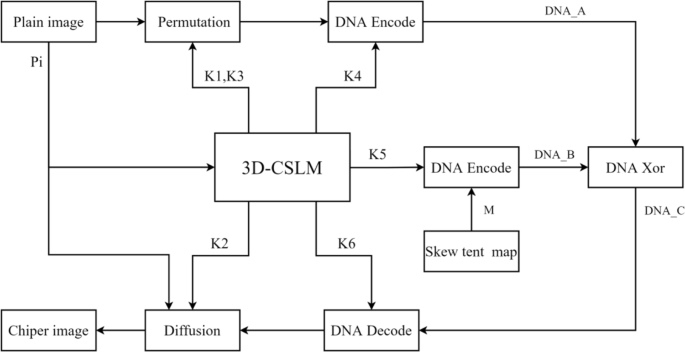
Encryption flow chart

-
Step 4.
Iterating 3D-CSLM generates multiple chaotic sequences {kx1, ky1, kz1, kx2, ky2, kz2}, the length of each sequence is M × N. Then treat these chaotic sequences as following equations, where Pi = mod (Pi, 256).
-
Step 5.
Permutation process. Input matrix P and sequence K1 and K3.
Firstly, perform column cyclic shift on matrix P. Perturb the pixel position of each column of the matrix according to Eq. (17), obtaining the preliminary scrambled matrix Pc. Then the row cyclic shift is carried out to change the pixel position of each row of the matrix, and the scrambled matrix Pl is obtained. Eq. (18) is the specific scrambling formula. circshift(⋅) is the displacement function.
-
Step 6.
Converts the digital matrix into DNA sequence. Input matrix Pl and sequence K4.
Firstly, convert the matrix Pl into a binary matrix, where each decimal value is converted to 8-bit binary number. Every 8 bits of binary would be converted to four bases, and the conversion rules are shown in Table 1. The conversion operation takes 8 bits as a group, M × N times in total, and the rules of each conversion are determined by sequence K4. Finally, obtain the transformed DNA sequence, DNA _ A. The operating formula could be described as follow,
-
Step 7.
Generate mask sequence. Input the initial key {μ, T1} into the Skew tent map, which is described as Eq. (20). Depending on this equation, generate a chaotic random sequence T. Then obtain mask sequence M by normalizing the values in sequence T between 0 and 255,
-
Step 8.
Perform DNA coding. Input mask sequence M and sequence K5.
Reshape the mask sequence M into a matrix Mr with size of M × N. Convert the mask matrix Mr into DNA sequence as the operations in Step 6, named DNA _ B, as Eq. (21) shows.
-
Step 9.
Perform DNA XOR Operation. Input the DNA sequencesDNA _ AandDNA _ B.
According to the computation rules showed in Table 2, two DNA sequences of the same size are subjected to the DNA XOR phase. DNA _ A is bitwise XORed with DNA _ B to produce a new DNA sequence DNA _ C. The operation could be described as follows in mathematically,
-
Step 10.
Perform DNA decoding operation to transform the DNA sequence DNA _ C into a decimal sequence D. Take every four bases as a group, using the DNA rules as showed in Table 1. The selection of DNA rules is determined by the sequence K6. After all bases are converted, a binary matrix will be obtained. Then convert the binary matrix into a decimal matrix D with size of M × N by using following equation,
-
Step 11.
Diffusion operation. Input matrix D, the sum of plain pixel values Pi, and sequence K2.
The purpose of this step is to associate with plain image information and improve the complexity of encrypted image C by adding random sequence K2. Firstly, calculate the values of C(1), then use these values to obtain the final encrypted image C.
The decryption process can be thought of as the inverse of the encryption process. Firstly, bring the transmitted key sequences into 3D-CSLM, generating multiple chaotic sequences. And then use Eqs. (11)–(16) to generate the needed random sequences. The second step is the inverse process of diffusion operation. Then the DNA coding step is carried out, the decimal matrix is converted into DNA sequence. Next, the reverse operation of DNA XOR is performed. After it, start the decoding step, obtaining the decimal matrix. Finally, the image pixels are restored to their original position by reverse permutation operation. The cipher image C would be decrypted as the original image P.
5 Experimental results and security analysis
All of the following experiments are performed in a computer with an Intel(R) Core (TM) i5-10210U CPU @ 1.60GHz 2.11 GHz and 8 GB of RAM, and the operating system is Microsoft Window10. And the software is MATLAB 2019a. The plain images which are used as examples, their size is 256 × 256. The encrypted and decrypted results are showed in Figs. 8 and 9. From the figures, it’s clear that whether ordinary grayscale images, all-white image or all-black image, the image encryption algorithm shows good performance.

Experimental results: (a) Lena; (b) cipher Lena; (c) decipher Lena; (d) Peppers; (e) cipher Peppers; (f) decipher Peppers; (g) Camera; (h) cipher Camera; (i) decipher Camera

Experimental results: (a) All-Black; (b) cipher All-Black; (c) decipher All-Black; (d) All-White; (e) cipher All-White; (f) decipher All-White
5.1 Key space analysis
The key space refers to the size of the digital space that can be used as the key. A good encryption algorithm should own large enough key space to resist exhaustive attack. The key values of the algorithm proposed in this paper are composed of the initial conditions of 3D-CSLM (a1, a2, a3, x1, y1, z1) and skew tent map (μ, T1). Assume that the current computer accuracy is 10−14, the key space would be (108)14 = 10112, which is more than the required 2100 [43]. Therefore, the proposed encryption scheme is strong enough to resist exhaustive attack and has high security.
5.2 Key sensitivity analysis
Key sensitivity refers to the degree of change of encrypted and decrypted images when the key is slightly changed. An excellent encryption algorithm owns a great difference in its encryption and decryption effect with small changes in the key. Figure 10 shows the key sensitivity experiment results of the encryption algorithm in this paper. The results indicate that when the precision is 10−14, the correct decryption image could not be recovered from the cipher image with slightly modifying keys, such as a1 = a1 + 10−14, x1 = x1 + 10−14, T1 = T1 + 10−14.

a Decryption with correct key, b Decryption with a1 + 10−14, c Decryption with x1 + 10−14, d Decryption with μ + 10−14, e Decryption with T1 + 10−14
5.3 Histogram analysis
The histogram shows the distribution of image pixel values. Ideally, the histogram of the encrypted image should be evenly distributed [40]. If the pixel value distribution is not uniform, the scheme is vulnerable to statistical analysis attack. A good encryption algorithm should make the cipher histogram tend to be balanced. The histograms of Lena, Pepper and Camera are showed as Fig. 11. It can be easily seen that the image histogram tends to be uniform after encryption process, indicating that the proposed scheme can resist statistical analysis attacks.

Histograms of the plain and cipher images. a Plain Lena, b Encrypted Lena, c Plain Peppers, d Encrypted Peppers, e Plain Camera, f Encrypted Camera
5.4 Correlation analysis
There is a high correlation between the adjacent pixels of the original image, which would influence greatly the security of encryption algorithms. In order to resist the attack of statistical analysis, the proposed encryption scheme should make the correlation coefficient of adjacent pixels in the encrypted image low enough. We utilize Eqs. (26)–(29) to calculate the correlation coefficient between adjacent pixels [39].
In the formula, x and y represent the pixel values of adjacent pixels, and K is the total number of pixels calculated. 3000 pairs of adjacent pixels in the horizontal, vertical and diagonal directions are randomly selected from the plain image and the cipher image, respectively, to compare the correlation between the adjacent pixels in the plain image and the cipher image. Figure 12 shows the pixel distribution of the plain image Lena and its encrypted image in all directions. Table 3 lists the experimental results of the correlation analysis. Table 4 compares the correlation coefficients of encrypted Lena images with other algorithms. Judging from the experimental results, the proposed algorithm is closer to zero compared with other algorithms. Thus, the proposed scheme can effectively reduce the correlation between pixels and has a better encryption effect than other schemes.

Correlation analysis diagrams: Horizontal direction of (a) plain Lena, (b) cipher Lena, Vertical direction of (c) plain Lena, (d) cipher Lena, Diagonal direction of (e) plain Lena, (f) cipher Lena
5.5 Differential attack analysis
The ideal encryption algorithm should have a significant difference in the encryption effect for the slight change of the plain image, resulting a good ability to resist the differential attack. NPCR (rate of change of pixel number) and UACI (uniform mean change intensity) are usually used to analyze the ability of the algorithm to resist differential attack [38]. The specific calculation equations are shown in Eqs. (30)–(32).
where M and N are the length and width of the original image, C1 and C2 are the cipher images whose plain images only with a pixel value difference. We randomly select a pixel from the plain image and add or subtract 1 from the original pixel value to achieve a tiny change effect of the image, obtaining two plain images which are used above. For a grayscale image with the size of 256 × 256, the ideal values of NPCR and UACI are 0.996093 and 0.334635, respectively. Tables 5 and 6 list the experimental results and comparisons with other algorithms. From the tow tables, it’s easy to find that the experimental results of our encryption algorithm are closer to the ideal value than others, so this scheme owns a good anti-differential attack performance.
5.6 Information entropy analysis
Information entropy can be used to evaluate the randomness degree of the image. The greater the randomness of the image pixel distribution, the higher the security. The information entropy is calculated by,
where L is the total number of pixels, S is the gray value, and p(si) is the probability of si occurrence. The theoretical value of information entropy of gray image is 8. Table 7 lists the information entropy results of this scheme, and Table 8 compares the information entropy of Lena image with other schemes. The experimental results in Tables 7 and 8 both show that the cipher image pixels are more random, and the proposed scheme has sufficient security.
5.7 Robustness analysis
The encrypted image may receive various interference factors during transmission, which will lead to the distortion of the encrypted image. Ideal encryption algorithm should have good robustness to resist various interference attacks. To prove the robustness of the image encryption, we perform the occlusion attack and noise attack to the encrypted image, respectively. Firstly, selecting the Peppers image as an example, we used 12.5%, 25%, and 50% occlusion attacks to it. The experimental results are showed as Fig. 13. It is not difficult to find that even if a large amount of data is lost in the central part of the encrypted image, the decrypted image can still recover many details of the original image.

Occlusion attack analysis: (a) encrypted image with 12.5% data loss, (b) encrypted image with 25% data loss, (c) encrypted image with 50% data loss, (d) decrypted image of (a), (e) decrypted image of (b), (f) decrypted image of (c)
Then, perform the noise test. Noise interference was added to the encrypted images, where salt & pepper noise (SPN) with intensity of 0.01, 0.03 and 0.05 was added to the Peppers images, respectively. Figure 14 shows the experimental effect. Although adding different noise interference, the decrypted image can still clearly show the original image details. Experimental results show that the algorithm in this paper has excellent robustness and can effectively resist jamming attacks.

Noise attack analysis: (a) encrypted image with 0.01 SPN, (b) encrypted image with 0.03 SPN, (c) encrypted image with 0.05 SPN, (d) decrypted image of (a), (e) decrypted image of (b), (f) decrypted image of (c)
5.8 Algorithm complexity analysis
The time complexity analysis is carried out for the encryption operation of the image with the size of M × N. The first stage is the sequence generation stage of the chaotic system, which produces random sequences with the length of M × N. In the permutation stage, the number of calculated execution operations is M + N. The time complexity of the encoding and decoding of DNA sequence and the process of DNA XOR operation is still O(M × N). The final XOR operation is executed for M × N times in total. Overall, the time complexity of the algorithm in this paper is O(M × N).
6 Conclusions
In this work, a model of constructing high-dimensional chaotic cyclic symmetric chaotic map by using low dimensional chaotic map is proposed. The model is generated by the cyclic symmetry of one-dimensional chaotic map. According to this model, two new chaotic maps 3D-CSLM and 3D-CSCM are proposed. Phase diagram, bifurcation diagram, Lyapunov exponent and Approximate entropy are provided to evaluate that the new maps have better ergodicity, wider chaotic range and higher complexity. Then we apply the new chaotic map, 3D-CSLM, to image encryption, designing a new image encryption algorithm based on it. In this algorithm, 3D-CSLM is used to generate chaotic sequences,combined with DNA method to improve the computational efficiency, and uses DNA XOR process to complete the diffusion operation between DNA elements. Simulation experiments were performed to illustrate that the algorithm has strong anti-attack ability and can resist different types of attacks such as differential attacks and noise attacks. Performance analysis shows that the algorithm has an excellent performance in terms of key space, key sensitivity, histogram, correlation analysis and information entropy.
The above conclusions and analysis indicates the good effects and the prospects for the real world application of the model, but there are still spaces to be explored and improved. Firstly, the model is more suitable for simple 1D chaotic mapping, and there are limitations for some complex 1D chaotic mappings. In addition, the proposed algorithm is mainly for gray image. For color image, it needs to be converted into gray image first. In the future, we will further study and optimize the proposed model and algorithm.
References
Aasawari S, Dolendro S (2020) Multiple images encryption based on 3D scrambling and hyper-chaotic system. Inf Sci 550:252–267
Alghafis A, Firdousi F, Khan M, Batool SI, Amin M (2020) An efficient image encryption scheme based on chaotic and deoxyribonucleic acid sequencing. Math Comput Simul 177:441–466
Brahim AH, Pacha AA, Said NH (2020) Image encryption based on compressive sensing and chaos systems. Optics Laser Technol 132:106489
Chatterjee I (2021) Artificial intelligence and patentability: review and discussions. Int J Modern Res 1:15–21
Chen LP, Yin H, Yuan LG, Lopes AM, Machado JAT, Wu RC (2020) A novel color image encryption algorithm based on a fractional-order discrete chaotic neural network and DNA sequence operations. Frontiers Inf Technol Electron Eng 21(6):866–879
Dehghani M, Montazeri Z, Dhiman G, Malik OP, Morales-Menendez R, Ramirez-Mendoza RA, Dehghani A, Guerrero JM, Parra-Arroyo L (2020) A spring search algorithm applied to engineering optimization problems. Appl Sci 10(18):6173
Dehghani M, Montazeri Z, Givi H et al (2020) Darts game optimizer: a new optimization technique based on darts game. Int J Intell Eng Syst 13(5):286–294
Dhiman G (2019) ESA: a hybrid bio-inspired metaheuristic optimization approach for engineering problems, Eng Comput 1–31
Dhiman G, Kaur A (2019) STOA: a bio-inspired based optimization algorithm for industrial engineering problems. Eng Appl Artif Intell 82:148–174
Dhiman G, Kumar V (2017) Spotted hyena optimizer: a novel bio-inspired based metaheuristic technique for engineering applications. Adv Eng Softw 114:48–70
Dhiman G, Kumar V (2018) Emperor penguin optimizer: a bio-inspired algorithm for engineering problems. Knowl-Based Syst 159:20–50
Dhiman G, Kumar V (2019) Seagull optimization algorithm: theory and its applications for large-scale industrial engineering problems. Knowl-Based Syst 165:169–196
Dhiman G, Garg M, Nagar A, Kumar V, Dehghani M (2020) A novel algorithm for global optimization: rat swarm optimizer. J Ambient Intell Humaniz Comput:1–26
Dhiman G, Oliva D, Kaur A, Singh KK, Vimal S, Sharma A, Cengiz K (2021) BEPO: a novel binary emperor penguin optimizer for automatic feature selection. Knowl-Based Syst 211:106560
El-Latif AAA, Li L, Zhang TJ, Wang N, Song XH, Niu XM (2012) Digital image encryption scheme based on multiple chaotic systems. Sens Imaging 13:67–88
Farah MAB, Guesmi R, Kachouri A, Samet M (2020) A novel chaos based optical image encryption using fractional Fourier transform and DNA sequence operation. Opt Laser Technol 121:105777
Han CY (2019) An image encryption algorithm based on modified logistic chaotic map. Optik. 181:779–785
Hua ZY, Zhu ZH, Yi S, Zhang Z, Huang HJ (2021) Cross-plane colour image encryption using a two-dimensional logistic tent modular map. Inf Sci 546:1063–1083
Huo DM, Zhou DF, Sheng Y, Yi SL, Zhang LZ, Zhou X (2019) Image encryption using exclusive-OR with DNA complementary rules and double random phase encoding. Phys Lett A 383(9):915–922
Iqbal N et al (2021) Dynamic 3D scrambled image based RGB image encryption scheme using hyperchaotic system and DNA encoding. J Inf Secur Appl 58:102809
Jain K, Aji A (2021) Krishnan P, Medical Image Encryption Scheme Using Multiple Chaotic Maps, Pattern Recognition Lett
Kaur M, Singh D, Sun K, Rawat U (2020) Color image encryption using non-dominated sorting genetic algorithm with local chaotic search based 5D chaotic map. Futur Gener Comput Syst 107:333–350
Kaur S, Awasthi LK, Sangal AL, Dhiman G (2020) Tunicate swarm algorithm: a new bio-inspired based metaheuristic paradigm for global optimization. Eng Appl Artif Intell 90:103541
Khalil N, Sarhan A (2021) Alshewimy M a M, an efficient color/grayscale image encryption scheme based on hybrid chaotic maps. Opt Laser Technol 143:107326
Kumar R, Dhiman G (2021) A comparative study of fuzzy optimization through fuzzy number. Int J Modern Res 1:1–14
Liu HJ, Wang XY (2011) Color image encryption using spatial bit-level permutation and high-dimension chaotic system. Opt Commun 284:3895–3903
Ma YL, Li CQ, Ou B (2020) Cryptanalysis of an image block encryption algorithm based on chaotic maps. J Inf Secur Appl 54:102566
Maddodi G, Awad A, Awad D, Awad M, Lee B (2018) A new image encryption algorithm based on heterogeneous chaotic neural network generator and dna encoding. Multimed Tools Appl 77(19):24701–24725
Mahmud M, Rahman A, Lee M, Choi JY (2020) Evolutionary-based image encryption using RNA codons truth table. Opt Laser Technol 121:105818
Malik DS, Shah T (2020) Color multiple image encryption scheme based on 3D-chaotic maps. Math Comput Simul 178:646–666
Mansouri A, Wang XY (2020) A novel one-dimensional sine powered chaotic map and its application in a new image encryption scheme. Inf Sci 520:46–62
Nezhad SYD, Safdarian N, Zadeh SAH (2020) New method for fingerprint images encryption using DNA sequence and chaotic tent map. Optik 224:165661
Patro KAK, Acharya B (2019) An efficient colour image encryption scheme based on 1-D chaotic maps. J Inf Secur Appl 46:23–41
Patro KAK, Soni A, Netam PK, Acharya B (2020) Multiple grayscale image encryption using cross-coupled chaotic maps. J Inf Secur Appl 52:102470
Sang Y, Sang J, Alam M S (2021) Image Encryption Based on Logistic Chaotic Systems and Deep Autoencoder, Pattern Recognition Lett
Short KM (1994) Steps toward unmasking secure communications. Int J Bifurcation Chaos 4(04):959–977
Vaishnav PK, Sharma S, Sharma P (2021) Analytical review analysis for screening COVID-19. Int J Modern Res 1:22–29
Wang XY, Guan NN (2020) Chaotic image encryption algorithm based on block theory and reversible mixed cellular automata. Opt Laser Technol 132:106501
Wang T, Wang MH (2020) Hyperchaotic image encryption algorithm based on bit-level permutation and DNA encoding. Opt Laser Technol 132:106355
Wang XY, Zhang JJ, Cao GH (2019) An image encryption algorithm based on ZigZag transform and LL compound chaotic system. Opt Laser Technol 119:105581
Wang MX, Wang XY, Zhao TT, Zhang C, Xia ZQ, Yao NM (2021) Spatiotemporal chaos in improved cross coupled map lattice and its application in a bit-level image encryption scheme. Inf Sci 544:1–24
Wu XJ, Wang KS, Wang XY, Kan HB, Kurths J (2018) Color image encryption using NCA map-based CML and one time keys. Signal Process 148:272–287
Wu JH, Liao XF, Yang B (2018) Image encryption using 2D Hénon-sine map and DNA approach. Signal Process 153:11–23
Xiong ZG, Wu Y, Ye CH, Zhang XM, Xu F (2019) Color image chaos encryption algorithm combining CRC and nine palace map. Multimed Tools Appl 78(22):31035–31055
Ye H, Zhou N, Gong L (2020) Multi-image compression-encryption scheme based on quaternion discrete fractional Hartley transform and improved pixel adaptive diffusion. Signal Process 175:107652–107666
Zeidabadi FA, Doumari SA, Dehghani M et al (2022) MLA: A New Mutated Leader Algorithm for Solving Optimization Problems. CMC-Comput Mater Continua 70(3):5631–5649
Zhang Q (2013) X P Wei, RGB color image encryption method based on Lorenz chaotic system and DNA computation. IETE Tech Rev 30(5):404–409
Zhang YQ, Wang XY, Xiu J, Chai ZL (2016) An image encryption scheme based on the MLNCML system using DNA sequences. Opt Lasers Eng 82:95–103
Zhang XC, Han F, Niu Y (2017) Chaotic image encryption algorithm based on bit permutation and dynamic DNA encoding. Comput Intell Neurosci 2017:6919675
Zhang YQ, He Y, Li P, Wang XY (2020) A new color image encryption scheme based on 2DNLCML system and genetic operations. Opt Lasers Eng 128:106040
Zhu H et al (2021) A three-dimensional bit-level image encryption algorithm with Rubik’s cube method. Math Comput Simul 185:754–770
Acknowledgements
This work is supported by the National Natural Science Foundation of China (61862042). Yingpeng Zhang and Hongyue Xiang are co-first authors.
Author information
Authors and Affiliations
Corresponding author
Ethics declarations
Conflict of interest
The authors declare that they have no conflicts of interest.
Additional information
Publisher’s note
Springer Nature remains neutral with regard to jurisdictional claims in published maps and institutional affiliations.
Rights and permissions
Springer Nature or its licensor holds exclusive rights to this article under a publishing agreement with the author(s) or other rightsholder(s); author self-archiving of the accepted manuscript version of this article is solely governed by the terms of such publishing agreement and applicable law.
About this article

Cite this article
Zhang, Y., Xiang, H., Zhang, S. et al. Construction of high-dimensional cyclic symmetric chaotic map with one-dimensional chaotic map and its security application. Multimed Tools Appl 82, 17715–17740 (2023). https://doi.org/10.1007/s11042-022-14044-y
Received:
Revised:
Accepted:
Published:
Issue Date:
DOI: https://doi.org/10.1007/s11042-022-14044-y