Optimal control of the stationary Kirchhoff equation

Abstract

We consider an optimal control problem for the steady-state Kirchhoff equation, a prototype for nonlocal partial differential equations, different from fractional powers of closed operators. Existence and uniqueness of solutions of the state equation, existence of global optimal solutions, differentiability of the control-to-state map and first-order necessary optimality conditions are established. The aforementioned results require the controls to be functions in $H^1$ and subject to pointwise lower and upper bounds. In order to obtain the Newton differentiability of the optimality conditions, we employ a Moreau–Yosida-type penalty approach to treat the control constraint and study its convergence. The first-order optimality conditions of the regularized problems are shown to be Newton differentiable, and a generalized Newton method is detailed. A discretization of the optimal control problem by piecewise linear finite elements is proposed and numerical results are presented.

1 Introduction

In this paper we study an optimal control problem governed by a nonlinear, nonlocal partial differential equation (PDE) of Kirchhoff-type

(1.1)

here $\varOmega \subset \mathbb {R}^N$ is an open and bounded set and the right-hand side f belongs to $L^2(\varOmega )$. We focus on the particular case $M(x,s;u) = u(x) + b(x) \, s$, which has been considered previously, e. g., in [8, 10]. Here u and b are strictly positive functions and u serves as the control. The full set of assumptions is given in Sect. 2. We mention that in case u and b are positive constants, (1.1) has a variational structure; see [10].

Equation (1.1) is the steady-state problem associated with its time-dependent variant

(1.2)

In one space dimension, problem (1.2) models small vertical vibrations of an elastic string with fixed ends, when the density of the material is not constant. Specifically, the control u is proportional to the inverse of the string’s cross section; see [10, 18]. A physical interpretation of the multi-dimensional problems (1.1) and (1.2) appears to be missing in the literature.

PDEs with nonlocal terms play an important role in physics and technology and they can be mathematically challenging. Although in some cases variational reformulations are available, the models (1.1), (1.2) do not allow this in general. Thus, despite the deceptively simple structure, (1.1) requires a set of analytical tools not often employed in PDE-constrained optimization. Existence and uniqueness of solutions for (1.1) have been investigated in [10] and [8]; see also the references therein. For further applications of nonlocal PDEs, we refer the reader to [2, 9, 17].

The authors in [8] studied an optimal control problem for (1.1) with the following cost functional

(1.3)

with an admissible set . However we believe that the proof of existence of an optimal solution in this work has a flaw. We give further details in the “Appendix”. Moreover, the proof in [8] is explicitly tailored to such tracking type functionals. In the present work we see it necessary to modify the control cost term to contain the stronger $H^1$-norm. We also allow for a more general state dependent term, which leads to the objective

(1.4)

and a set of admissible controls in $H^1(\varOmega )$. In this setting, we prove the weak-strong continuity of the control-to-state operator into $H^1_0(\varOmega ) \cap W^{2,q}(\varOmega )$ for any $q\in [1,\infty )$ and the existence of a globally optimal solution. Moreover, we work with a pointwise lower bound on admissible controls. This bound has an immediate technological interpretation, representing an upper bound on the string’s cross section. On the other hand, we also impose an upper bound on the controls. This is to be able to use the topology of $L^\infty (\varOmega )$ in the proof of the Fréchet differentiability of the control-to-state map so that we can derive optimality conditions in a more straightforward way than by the Dubovitskii-Milyoutin formalism utilized in [8].

The first-order optimality conditions obtained when minimizing (1.4) subject to (1.1) involve a variational inequality of nonlinear obstacle type in $H^1$. We choose to relax and penalize the bound constraints via a Moreau–Yosida regularization, which amounts to a quadratic penalty of the bound constraints for the control. In this setting, we can prove the generalized (Newton) differentiability of the optimality system. A similar philosophy, albeit for a different problem, has been pursued by [1]. We also mention [23, Chapter 9.2] for an approach via a regularized dual obstacle problem. A recent and promising alternative is offered by [5], where the Newton differentiability of the solution map for unilateral obstacle problems is shown, without the need to penalize the constraint. Indeed, relaxing the lower and upper bounds adds new difficulties, since the existence of a solution of the Kirchhoff equation (1.1) can only be guaranteed for positive controls. Therefore, we compose the control-to-state map with a smooth cut-off function. We then study the convergence of global minimizers as the penalty parameter goes to zero, see Theorem 3.4 for details. We can expect a corresponding result to hold also for locally optimal solutions under an assumption of second-order sufficient optimality conditions, but this is not investigated here.

To summarize our contributions in comparison to [8], we consider a more general objective, present a simpler proof for the existence of a globally optimal control, prove the differentiability of the control-to-state map and generalized differentiability of the optimality system for a regularized version of the problem as well as the applicability of a generalized Newton scheme. We also describe a structure preserving finite element discretization of the problem and the discrete counterpart of the generalized Newton method.

The paper is organized as follows. In Sect. 2, we review existence and uniqueness results for solutions of the Kirchhoff equation (1.1) and prove the existence of a globally optimal control. Subsequently, we prove the Fréchet differentiability of the control-to-state operator and derive a system of necessary optimality conditions for a regularized problem in Sect. 3. In Sect. 4, we prove the Newton differentiability of the optimality system and devise a locally superlinearly convergent scheme in appropriate function spaces. Section 5 addresses the discretization of the optimal control problem, its optimality system and the generalized Newton method by a finite element scheme. The paper concludes with numerical results in Sect. 6.

2 Optimal control problem: existence of a solution

In this work we are interested in the study of the following optimal control problem for a stationary nonlinear, nonlocal Kirchhoff equation:

(2.1a)

(2.1b)

(2.1c)

The set of admissible controls is given by

(2.2)

The following are our standing assumptions.

Assumption 2.1

We assume that $\varOmega \subset \mathbb {R}^N$ is a bounded domain of class $C^{1,1}$ with $1 \le N \le 3$; see for instance [22, Chapter 2.2.2]. The control cost parameter $\lambda$ is a positive number. The right-hand side f is a given function in $L^\infty (\varOmega )$ satisfying $f \ge f_0$ a.e., where $f_0$ is a non-negative real number. The bounds $u_a$ and $u_b$ are functions in $C({\overline{\varOmega }})$ such that $u_b \ge u_a \ge u_0$ holds for some positive real number $u_0$. Finally, we assume $b \in L^\infty (\varOmega )$ with $b \ge b_0$ a.e. for some positive real number $b_0$.

The integrand $\varphi$ in the objective is assumed to satisfy the following standard assumptions; see for instance [22, Chapter 4.3]:

Assumption 2.2

   

• (1) $\varphi :\varOmega \times \mathbb {R}\rightarrow \mathbb {R}$ is Carathéodory and of class $C^2$, i. e.,

  • (i) $\varphi (\cdot , y) :\varOmega \rightarrow \varphi (x,y)$ is measurable for all $y\in \mathbb {R}$,

  • (ii) $\varphi (x,\cdot ) :\mathbb {R}\rightarrow \varphi (x,y)$ is twice continuously differentiable for a.e. $x\in \varOmega$.

• (2) $\varphi$ satisfies the boundedness and local Lipschitz conditions of order 2, i. e., there exists a constant $K > 0$ such that

  

  and for every $M > 0$, there exists a Lipschitz constant $L(M) > 0$ such that

  

  holds for a.e. $x\in \varOmega$ and for all , $i=1,2$.

Assumption 2.2 implies the following properties for the Nemytskii operator $\varPhi (y)(x) {:}{=}\varphi (x,y(x))$.

Lemma 2.3

([22, Lemma 4.11, Lemma 4.12]).

• (i) $\varPhi$ is continuous in $L^\infty (\varOmega )$. Moreover, for all $r \in [1,\infty ]$, we have

  

  for all $y,z\in L^\infty (\varOmega )$ such that and

• (ii) $\varPhi$ is twice continuously Fréchet differentiable in $L^\infty (\varOmega )$, and we have

  

  for a.e. $x \in \varOmega$ and $h, h_1, h_2 \in L^\infty (\varOmega )$.

We now proceed to define the notion of weak solution of the Kirchhoff problem. Since for any pair $(u,y)\in \mathcal {U}_{\text {ad}}\times H^1(\varOmega )$, is strictly positive, we can write Eq. (2.1b) in the form

(2.3)

Here and in the following, we occasionally write instead of . The $L^2(\varOmega )$-inner product is denoted by . Moreover, we denote by $\mathcal {L}(U,V)$ the space of bounded linear operators from U to V.

Multiplication of (2.3) with a test function $v\in H^1_0(\varOmega )$ and integration by parts yields the following definition.

Definition 2.4

A function $y \in H^1_0(\varOmega )$ is called a weak solution of (2.3) if it satisfies

(2.4)

The existence of a unique weak solution as well as its $W^{2,q}(\varOmega )$-regularity has been shown in [8, Theorem 2.2]. Nevertheless, we briefly sketch the proof since its main idea is utilized again later on. For a complete proof we refer the reader to [8].

Theorem 2.5

For any $u \in \mathcal {U}_{\text {ad}}$, there exists a unique weak solution $y \in H^1_0(\varOmega )$ of the Kirchhoff problem (2.3). Moreover, $y \in W^{2,q}(\varOmega )$ holds for all $q\in [1,\infty )$, so it is also a strong solution.

Proof

Suppose that $u \in \mathcal {U}_{\text {ad}}$ and let $g :[0,\infty ) \rightarrow \mathbb {R}$ be the function defined by

where $y_s$ is the unique weak solution of the Poisson problem

$$\begin{aligned} \left\{ \begin{array}{ll} -\Delta y_s = \frac{f}{u + b \, s} &{}\quad \text {in } \varOmega , \\ y_s = 0 &{}\quad \text {on } \partial \varOmega . \end{array} \right. \end{aligned}$$

A monotonicity argument can be used to show that g has a unique root. Since $y_s$ solves (2.3) if and only if $g(s) = 0$ holds, the uniqueness of the solution of the Kirchhoff equation is guaranteed. Furthermore, due to the boundedness of u from below, the right-hand side $f / (u + b \, s)$ of the Poisson problem above belongs to $L^\infty (\varOmega )$. Hence, by virtue of regularity results for the Poisson problem, $y \in W^{2,q}(\varOmega )$ holds for any $q\in [1,\infty )$; see, e. g., [11, Theorem 9.15]. $\square$

For the proof of existence of a globally optimal control of (2.1), we show next that the control-to-state operator $S:\mathcal {U}_{\text {ad}}\rightarrow H^1_0(\varOmega ) \cap W^{2,q}(\varOmega )$ is continuous.

Theorem 2.6

The control-to-state map $S$ is continuous from $\mathcal {U}_{\text {ad}}$ (with the $L^2(\varOmega )$-topology) into $H^1_0(\varOmega ) \cap W^{2,q}(\varOmega )$ for all $q\in [1,\infty )$.

Proof

The control-to-state map $S:\mathcal {U}_{\text {ad}}\rightarrow H^1_0(\varOmega ) \cap W^{2,q}(\varOmega )$ is well-defined as a consequence of Theorem 2.5. To show its continuity, let $\{u_n\} \subset \mathcal {U}_{\text {ad}}$ be a sequence with $u_n \rightarrow u$ in $L^2(\varOmega )$. Set $y_n{:}{=}S(u_n)$, then we have the a-priori estimate

From now on, suppose without loss of generality that $q\in [2,\infty )$ holds. Since $W^{2,q}(\varOmega )$ is a reflexive Banach space and every bounded subset of a reflexive Banach space is weakly relatively compact, there exists a subsequence $y_n$, denoted by the same indices, satisfying $y_n \rightharpoonup {\hat{y}}$ in $W^{2,q}(\varOmega )$. The compactness of the embedding $W^{2,q}(\varOmega ) \hookrightarrow W^{1,q}(\varOmega )$ implies the strong convergence $y_n \rightarrow {\hat{y}}$ in $W^{1,q}(\varOmega )$ and thus . Moreover, $u_n \rightarrow u$ in $L^2(\varOmega )$ implies the existence of a further subsequence $u_n$, still denoted by the same indices, with $u_n(x) \rightarrow u(x)$ for a.e. $x \in \varOmega$. Consequently,

Since is dominated by $\frac{f}{u_a}$, we have

By virtue of the dominated convergence theorem,

On the other hand, from $y_n \rightharpoonup {\hat{y}}$ in $W^{2,q}(\varOmega )$, it follows that $\Delta y_n \rightharpoonup \Delta {\hat{y}}$ holds in $L^q(\varOmega )$. The uniqueness of the weak limit yields

and from the uniqueness of the solution of (2.3) we obtain ${\hat{y}} = S(u)$. Therefore, $\Delta y_n \rightarrow \Delta {\hat{y}}$ holds in $L^q(\varOmega )$ and thereby $y_n \rightarrow {\hat{y}}$ in $W^{2,q}(\varOmega )$.

We note that we have proved that for any sequence $\{u_n\} \subset \mathcal {U}_{\text {ad}}$ with $u_n \rightarrow u$ in $L^2(\varOmega )$ there exists a subsequence $\{u_{n}\}$, denoted by the same indices, so that $S(u_{n}) \rightarrow S(u)$ in $W^{2,q}(\varOmega )$. Thus we can easily conclude convergence of the entire sequence $S(u_n) \rightarrow S(u)$ in $W^{2,q}(\varOmega )$. Indeed, if $S(u_n) \not \rightarrow S(u)$, then there exist $\delta > 0$ and a subsequence with indices $n_k$ such that

Since $u_{n_k} \rightarrow u$ in $L^2(\varOmega )$, there exists a further subsequence $\{u_{n_{k_\ell }}\}$ such that $S(u_{n_{k_\ell }}) \rightarrow S(u)$, which is a contradiction. Consequently, we obtain $S(u_n) \rightarrow S(u)$ as claimed. $\square$

The compact embedding $H^1(\varOmega ) \hookrightarrow L^2(\varOmega )$ immediately leads to the following corollary.

Corollary 2.7

The control-to-state map $S$ is weakly-strongly continuous from $\mathcal {U}_{\text {ad}}$ (with the $H^1(\varOmega )$-topology) into $H^1_0(\varOmega ) \cap W^{2,q}(\varOmega )$ for all $q\in [1,\infty )$. That is, when $\{u_n\} \subset \mathcal {U}_{\text {ad}}$ with $u_n \rightharpoonup u$ in $H^1(\varOmega )$, then $S(u_n) \rightarrow S(u)$ in $W^{2,q}(\varOmega )$.

We can now address the existence of a global minimizer of (2.1).

Theorem 2.8

Problem (2.1) possesses a globally optimal control ${\bar{u}} \in \mathcal {U}_{\text {ad}}$ with associated optimal state ${\bar{y}} = S({\bar{u}}) \in H^1_0(\varOmega ) \cap W^{2,q}(\varOmega )$ for all $q\in [1,\infty )$.

Proof

The proof follows the standard route of the direct method so we can be brief.

• Step (1): We show that the reduced cost functional

  

  is bounded from below on the set $\mathcal {U}_{\text {ad}}$. To this end, recall from the proof of Theorem 2.6 that $S(\mathcal {U}_{\text {ad}})$ is bounded in $W^{2,q}(\varOmega )$. Due to the embedding $W^{2,q}(\varOmega ) \hookrightarrow C({\overline{\varOmega }})$ for $q> N / 2$, there exists $M > 0$ such that holds for all $u \in \mathcal {U}_{\text {ad}}$. From Assumption 2.2 we can obtain the estimate

  

  This implies

  

  (2.5)

  for all $u \in \mathcal {U}_{\text {ad}}$. The assertion follows.

• Step (2): We construct the tentative minimizer ${\bar{u}}$. Since j is bounded from below on $\mathcal {U}_{\text {ad}}$, there exists a minimizing sequence $\{u_n\} \subset \mathcal {U}_{\text {ad}}$ so that

  $$\begin{aligned} j(u_n) \searrow \inf _{u \in \mathcal {U}_{\text {ad}}} j(u) {=}{:}\beta . \end{aligned}$$

  The boundedness of $\{u_n\}$ in $H^1(\varOmega )$ follows from the radial unboundedness of j. Consequently, there exists a subsequence, denoted by the same indices, such that $u_n \rightharpoonup {\bar{u}}$ in $H^1(\varOmega )$. $\mathcal {U}_{\text {ad}}$ is convex and closed in $H^1(\varOmega )$ and therefore weakly closed in $H^1(\varOmega )$, thus ${\bar{u}} \in \mathcal {U}_{\text {ad}}$. Now Corollary 2.7 implies $S(u_n) \rightarrow S({\bar{u}})$ in $W^{2,q}(\varOmega )$.

• Step (3): It remains to show the global optimality of ${\bar{u}}$. Set $F(y) {:}{=}\int _\varOmega \varPhi (y) \mathop {}\!\text {d}x$, thus F is composed of a Nemytskii operator and a continuous linear integral operator from $L^1(\varOmega )$ into $\mathbb {R}$. By virtue of Lemma 2.3, $\varPhi$ is continuous in $L^\infty (\varOmega )$. Since $W^{2,q}(\varOmega ) \hookrightarrow L^\infty (\varOmega )$ holds, $F \circ S$ is weakly-strongly continuous on $\mathcal {U}_{\text {ad}}$ w.r.t. the topology of $H^1(\varOmega )$.

  In summary, exploiting the weak sequential lower semicontinuity of we have

  

  By definition of $\beta$ and since ${\bar{u}} \in \mathcal {U}_{\text {ad}}\cap H^1(\varOmega )$, we therefore must have $\beta = j({\bar{u}})$. $\square$

Remark 2.9

An inspection of the existence theory shows that these results remain valid in the absence of an upper bound $u_b$ on the control. However, the upper bound is of essential importance in the following section, where we prove the Fréchet differentiability of the control-to-state map.

3 Optimality system

In this section we address first-order necessary optimality conditions for local minimizers. We need to overcome several obstacles. First of all, the control-to-state operator

$$\begin{aligned} S :\mathcal {U}_{\text {ad}}\rightarrow H^1_0(\varOmega ) \cap W^{2,q}(\varOmega ) \end{aligned}$$

is not Fréchet differentiable in the $H^1(\varOmega )$-topology. The reason is that $\mathcal {U}_{\text {ad}}$ has empty interior w.r.t. this topology except in dimension $N = 1$. More precisely, every $H^1(\varOmega )$-neighborhood of any control $u \in \mathcal {U}_{\text {ad}}$ contains functions which are arbitrarily negative on sets of small but positive measure. However, the proof of Theorem 2.5, which establishes the well-definedness of the control-to-state map, is contingent upon the controls to remain positive. In order to overcome this issue, we work with the topology of $H^1(\varOmega ) \cap L^\infty (\varOmega )$.

With regard to an efficient numerical solution method in function spaces, we are aiming to arrive at an optimality system which is Newton differentiable. To this end, we propose to relax and penalize the control constraint. Notice that this is not straightforward since we need to ensure positivity of the relaxed control in the state equation. We achieve the latter by a smooth cut-off function. The optimality system of the penalized problem then turns out to be Newton differentiable, as we shall show in Sect. 4.

The material in this section is structured as follows. In Sect. 3.1, we prove the Fréchet differentiability of the control-to-state map. We establish the system of first-order necessary optimality conditions for the original problem (2.1) in Sect. 3.2. In Sect. 3.3 we introduce the penalty approximation and show that for any null sequence of penalty parameters, there exists a subsequence of global solutions to the corresponding penalized problems which converges weakly to a global solution of the original problem; see Theorem 3.4. Section 3.4 addresses the system of first-order necessary optimality conditions for the penalized problem.

3.1 Differentiability of the control-to-state map

In this subsection we show the Fréchet differentiability of the control-to-state map $S$ by means of the implicit function theorem. To verify the assumption of the implicit function theorem, we need the following result about the linearization of the Kirchhoff equation (2.3).

Proposition 3.1

Suppose that ${\hat{u}} \in \mathcal {U}_{\text {ad}}$ and ${\hat{y}} \in H^1_0(\varOmega ) \cap W^{2,q}(\varOmega )$ is the associated unique solution of the Kirchhoff equation (2.3) for any $q\in [1,\infty )$. Then, for any $h \in L^q(\varOmega )$, the linearized problem

(3.1)

has a unique solution $y \in H^1_0(\varOmega ) \cap W^{2,q}(\varOmega )$.

Proof

Since (3.1) is linear, we can decompose it into two problems with right hand sides $h^+ {:}{=}\max \{0,h\}$ and $h^- {:}{=}- \min \{0,h\}$ respectively. To each of these problems, an argument similar to the proof of Theorem 2.5 applies, and we obtain unique weak solutions $y^+$ and $y^-$ which belong to $H^1_0(\varOmega ) \cap W^{2,q}(\varOmega )$. Then clearly, $y = y^+ - y^-$ solves (3.1). $\square$

Theorem 3.2

Suppose that ${\hat{u}} \in \mathcal {U}_{\text {ad}}$. Then the control-to-state operator

$$\begin{aligned} S:\mathcal {U}_{\text {ad}}\rightarrow H^1_0(\varOmega ) \cap W^{2,q}(\varOmega ) \end{aligned}$$

is continuously Fréchet differentiable w.r.t. the topology of $L^\infty (\varOmega )$ on an open $L^\infty (\varOmega )$-neighborhood of ${\hat{u}}$ for all $q\in [1,\infty )$.

Proof

Suppose that ${\hat{u}} \in \mathcal {U}_{\text {ad}}$ is arbitrary and that ${\hat{y}} \in H^1_0(\varOmega ) \cap W^{2,q}(\varOmega )$ is the associated state. The map defined by

is continuously Fréchet differentiable with

It remains to show that has a bounded inverse. To this end, consider

(3.2)

The existence and uniqueness of $y \in H^1_0(\varOmega ) \cap W^{2,q}(\varOmega )$ satisfying (3.1), i. e., $E_y({\hat{y}},{\hat{u}}) \, y = h$, is established by virtue of Proposition 3.1. This implies the bijectivity of $E_y({\hat{y}},{\hat{u}})$. The open mapping/continuous inverse theorem now yields that the inverse of $E_y({\hat{y}},{\hat{u}})$ is continuous. Notice that $E(y,u) = 0 \Leftrightarrow E(S(u),u) = 0$ holds for all $u \in \mathcal {U}_{\text {ad}}$. Invoking the implicit function theorem, we obtain that $S$ is continuously differentiable in some $L^\infty (\varOmega )$-neighborhood of ${\hat{u}}$. Since ${\hat{u}} \in \mathcal {U}_{\text {ad}}$ was arbitrary, $S$ actually extends into an $L^\infty (\varOmega )$-neighborhood of $\mathcal {U}_{\text {ad}}$ and it is continuously differentiable there. Moreover, we obtain that $\delta y = S'({\hat{u}}) \, \delta u$ satisfies $E_y({\hat{y}}, {\hat{u}}) \, \delta y = - E_u({\hat{y}}, {\hat{u}}) \, \delta u$, i. e.,

$\square$

3.2 First-order optimality conditions

The optimality system can be derived by using the Lagrangian $\mathcal {L}:H^1_0(\varOmega ) \times \mathcal {U}_{\text {ad}}\times H^1_0(\varOmega ) \rightarrow \mathbb {R}$, defined by

(3.3)

and taking the derivative with respect to the state and the control. In the first case, we obtain

for $\delta y \in H^1_0(\varOmega ) \cap W^{2,q}(\varOmega )$. Integration by parts yields

Notice that $\mathcal {L}_y(y, u, p)\, \delta y = 0$ for all $\delta y \in H^1_0(\varOmega ) \cap W^{2,q}(\varOmega )$ represents the strong form of the adjoint equation, which reads

(3.4)

We point out that (3.4) is again a nonlocal equation. Given $u \in \mathcal {U}_{\text {ad}}$ and $y \in H^1_0(\varOmega ) \cap W^{2,q}(\varOmega )$, (3.4) has a unique solution $p \in H^1_0(\varOmega ) \cap W^{2,q}(\varOmega )$. This can be shown either by direct arguments as in Theorem 2.5, or by exploiting that the bounded invertibility of $E_y$ implies that of its adjoint, see the proof of Theorem 3.2.

The derivative of the Lagrangian with respect to the control is given by

for $\delta u \in H^1(\varOmega )$.

It is now standard to derive the following system of necessary optimality conditions.

Theorem 3.3

Suppose that is a locally optimal solution of problem (2.1) for any $q\in [1,\infty )$. Then there exists a unique adjoint state $p \in H^1_0(\varOmega ) \cap W^{2,q}(\varOmega )$ for all $q\in [1,\infty )$ such that the following system holds:

(3.5a)

(3.5b)

(3.5c)

Notice that (3.5b) is a nonlinear obstacle problem for the control variable u originating from the bound constraints in $\mathcal {U}_{\text {ad}}$ and the presence of the $H^1$-control cost term in the objective. Until recently, the Newton differentiability of the associated solution map was not known. In order to apply a generalized Newton method, we therefore chose to relax and penalize the bound constraints via a quadratic penalty in the following section. This is also known as Moreau–Yosida regularization of the indicator function pertaining to $\mathcal {U}_{\text {ad}}$.

Recently, the authors in [5] proved a Newton differentiability result for the solution map of unilateral obstacle problems. This approach offers a promising alternative route to solving (3.5) numerically. It would amount to introducing a fourth unknown satisfying and replacing (3.5b) by $u = G(z)$, where G stands for the solution map of the obstacle problem

$$\begin{aligned} \lambda \int _\varOmega \nabla u \cdot (\nabla v - u) + u \, (v - u) - z \, (v - u) \, \mathop {}\!\text {d}x\ge 0 \quad \text {for all } v \in \mathcal {U}_{\text {ad}}. \end{aligned}$$

We leave the details for future work.

3.3 Moreau–Yosida penalty approximation

The Moreau–Yosida penalty approximation of problem (2.1) consists of the following modifications.

• (1) We remove the constraints $u_a \le u \le u_b$ from $\mathcal {U}_{\text {ad}}$ and work with controls in $H^1(\varOmega )$ which do not necessarily belong to $L^\infty (\varOmega )$.

• (2) We add the penalty term to the objective. Here $v_+ = \max \{0,v\}$ is the positive part function and $\varepsilon > 0$ is the penalty parameter.

• (3) We replace the control-to-state relation $y = S(u)$ by

  

  where $\eta _\varepsilon$ is a family of monotone and convex $C^3$ approximations of the positive part function satisfying $\eta _\varepsilon (t) = t$ for $t > \varepsilon$, $\eta _\varepsilon (t) = 0$ for $t < - \varepsilon$ for some $\varepsilon \in (0,u_0/2)$ and $\eta _\varepsilon ' \in [0,1]$ everywhere.

An example of such a function is $\eta _\varepsilon (t) = \varepsilon \, \eta (\frac{t}{\varepsilon })$, where

Notice that modification (3) is required since the control-to-state map S is guaranteed to be defined only for positive controls; compare Theorem 2.5. Therefore, we use $u_a / 2 + \eta _\varepsilon (u - u_a / 2) \ge u_a/2$ as an effective control. In addition, $u_a / 2 + \eta _\varepsilon (u - u_a / 2) = u$ holds for all $u \in \mathcal {U}_{\text {ad}}$, provided that $\varepsilon$ is small enough. We now consider the following relaxed problem:

The relation between (P$_\varepsilon$) and the original problem (2.1) is clarified in the following theorem.

Theorem 3.4

   

• (i) For all $\varepsilon > 0$, problem (P$_\varepsilon$) possesses a globally optimal solution for all $q\in [1,\infty )$.

• (ii) For any sequence $\varepsilon _n \searrow 0$, there is a subsequence of which converges weakly to some in $W^{2,q}(\varOmega ) \times H^1(\varOmega )$. Moreover, $u^* \in \mathcal {U}_{\text {ad}}$ holds and is a globally optimal solution of (2.1).

Proof

Statement (i) can be proved in a straightforward manner using a similar procedure as in Theorem 2.8. The proof of statement (ii) is divided into several steps. As in the proof of Theorem 2.8, we define $\beta$ to be the globally optimal value of the objective in (2.1). Similarly, we let $\beta _\varepsilon$ denote the globally optimal value of the objective in (P$_\varepsilon$). Suppose that $\varepsilon _n \searrow 0$ is any sequence.

• Step (1): We show that is bounded in $W^{2,q}(\varOmega ) \times H^1(\varOmega )$.

  Suppose that $({\bar{y}}, {\bar{u}})$ is a globally optimal solution of (2.1). Owing to the definition of $\beta _\varepsilon$, we have

  

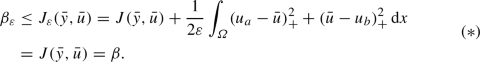
  The next-to-last equality is true since ${\bar{u}} \in \mathcal {U}_{\text {ad}}$ holds and therefore, the penalty term vanishes. Moreover, we obtain

  

  where the last inequality follows from (*). Since

  

  holds, we obtain as in the proof of Theorem 2.6. Therefore, ${\bar{y}}_{\varepsilon _n}$ is also bounded in $C({\overline{\varOmega }})$ and consequently, $\int _\varOmega \varphi (x,{\bar{y}}_{\varepsilon _n}) \mathop {}\!\text {d}x$ is bounded below, see (2.5). Finally,

  

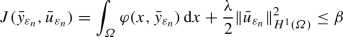
  implies that is bounded.

• Step (2): From Step (1) it follows that there exists a subsequence , denoted with the same subscript, such that in $W^{2,q}(\varOmega ) \times H^1(\varOmega )$. We show that $u^* \in \mathcal {U}_{\text {ad}}$ holds.

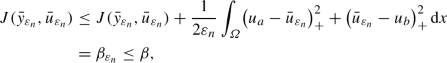
  We have already shown that $\beta _{\varepsilon _n} \le \beta$ holds, therefore

  

  Taking the $\limsup$ in this inequality as $n \rightarrow \infty$, we find

  

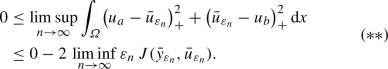
  From in $W^{2,q}(\varOmega ) \times H^1(\varOmega )$ we conclude ${\bar{u}}_{\varepsilon _n} \rightarrow u^*$ in $L^2(\varOmega )$ and

  $$\begin{aligned} J(y^*, u^*) \le \liminf _{n\rightarrow \infty } J({\bar{y}}_{\varepsilon _n}, {\bar{u}}_{\varepsilon _n})\qquad \qquad (***) \end{aligned}$$

  as in the proof of Theorem 2.8. Passing with $n \rightarrow \infty$ in (**) yields

  

  and consequently, $u^* \in \mathcal {U}_{\text {ad}}$ follows.

• Step (3): To obtain the convergence $\eta _{\varepsilon _n} ({\bar{u}}_{\varepsilon _n} - u_a/2) \rightarrow u^* - u_a/2$ in $L^2(\varOmega )$, it suffices to note that the assumptions on $\eta _\varepsilon$ imply that, for all $t \in \mathbb {R}$, $\eta _{\varepsilon _n}(t) \rightarrow \max \{0, t\}$ holds as $n \rightarrow \infty$ and that $\eta _{\varepsilon _n}$ has a Lipschitz constant of 1 for all n. In combination with $u^* \ge u_a$, the triangle inequality, and the dominated convergence theorem, this gives

  

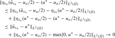
  as desired. The continuity of $S$ on $\mathcal {U}_{\text {ad}}$ w.r.t. the $L^2(\varOmega )$-topology now implies

  

  From Step (2) we have the weak convergence of ${\bar{y}}_{\varepsilon _n}$ to $y^*$. The uniqueness of the weak limit shows $y^* = S(u^*)$.

• Step (4): Since $J({\bar{y}}_{\varepsilon _n}, {\bar{u}}_{\varepsilon _n}) \le \beta$ holds, we obtain $J(y^*, u^*) \le \beta$ by invoking (***). Moreover, since $(y^*,u^*)$ is admissible for (2.1), the definition of $\beta$ implies $J(y^*,u^*) = \beta$, which completes the proof. $\square$

3.4 First-order optimality conditions for the penalized problem

The derivation of optimality conditions for (P$_\varepsilon$) proceeds along the same lines as in Sect. 3.2 and the details are omitted. Notice that the use of the cut-off function in the control-to-state map resolves the difficulty with differentiability of this map with respect to $H^1(\varOmega )$-topology in appropriate function spaces. For simplicity, we drop the index $\cdot _\varepsilon$ from now on and denote states, controls, and associated adjoint states by (y, u, p). We obtain the following regularized system of necessary optimality conditions.

Theorem 3.5

Suppose that is a locally optimal solution of problem (P$_\varepsilon$) for any $q\in [1,\infty )$. Then there exists a unique adjoint state $p \in H^1_0(\varOmega ) \cap W^{2,q}(\varOmega )$ for all $q\in [1,\infty )$ such that the following system holds:

(3.6a)

(3.6b)

(3.6c)

Remark 3.6

We note that under a second-order sufficient condition, which is not investigated in this paper, every solution of (3.6) is a strict local minimizer of (P$_\varepsilon$). According to Theorem 3.4, applied to a modified problem with a suitable localization term, the local minimizer of the penalized problem under consideration converges to a local minimizer of the original optimal control problem as $\varepsilon \rightarrow 0$. This technique is well known; see for instance [4, Section 4]. Therefore, under second-order sufficient optimality conditions, the solutions of the optimality system of (P$_\varepsilon$) converge to the solutions of the optimality system of (2.1).

Corollary 3.7

The terms

in (3.6b) belong to $L^\infty (\varOmega )$ and therefore, any locally optimal control of $(\textrm{P}_\varepsilon )$ belongs to $W^{2,q}(\varOmega )$ for any $q\in [1,\infty )$.

Proof

We only elaborate on the case $N = 3$ since the cases $N \in \{1,2\}$ are similar. We first consider the numerator of the first term. Here $f \in L^\infty (\varOmega )$ holds by Assumption 2.1 and $p \in L^\infty (\varOmega )$ by virtue of the embedding $W^{2,q}(\varOmega ) \hookrightarrow L^\infty (\varOmega )$ for $q> 3/2$. Moreover, $\eta _\varepsilon '$ maps into [0, 1] and therefore $\eta _\varepsilon '(u - u_a)$ belongs to $L^\infty (\varOmega )$ as well. The denominator is bounded below by $u_a/2$, and therefore, the first term belongs to $L^\infty (\varOmega )$.

The second term, , belongs to $L^6(\varOmega )$ due to the embedding $H^1(\varOmega ) \hookrightarrow L^6(\varOmega )$. Inserting this into (3.6b) with the differential operator $\lambda \, (-\Delta + id )$ and the remaining terms on the right-hand side shows $u \in W^{2,6}(\varOmega )$, which in turn embeds into $L^\infty (\varOmega )$.

Repeating this procedure one more time implies $u \in W^{2,q}(\varOmega )$. $\square$

4 Generalized Newton method

In this section we show that the optimality system (3.6) of the penalized problem is differentiable in a generalized sense, referred to as Newton differentiability. This allows us to formulate a generalized Newton method. Due to its similarity with the concept of semismoothness, see [23], such methods are sometimes referred to as a semismooth Newton method.

Definition 4.1

([13, Definition 1], [16, Definition 8.10]). Let X and Y be two Banach spaces and D be an open subset of X. The mapping $F :D \subset X \rightarrow Y$ is called Newton differentiable on the open subset $V \subset D$ if there exists a map $G :V \rightarrow \mathcal {L}(X,Y)$ such that, for every $x \in V$,

In this case G is said to be a Newton derivative of F on V.

We formulate the optimality system (3.6) in terms of an operator equation $F = 0$ where

(4.1)

and $q\in [\max \{1,N/2\},\infty )$ is arbitrary but fixed.

Here $W^{2,q}_\diamond (\varOmega )$ is defined as

The component $F_1$ represents the adjoint equation (3.6a) in strong form, i. e.,

The continuous Fréchet differentiability of $F_1$ is a standard result, which uses Lemma 2.3 and the embedding $W^{2,q}(\varOmega ) \hookrightarrow L^\infty (\varOmega )$. The directional derivative is given by

Similarly, $F_3$ represents the state equation (3.6c), i. e.,

and its continuous Fréchet derivative is given by

Finally, in order to define $F_2$ we integrate (3.6b) by parts, which is feasible due to Corollary 3.7. This results in the equivalent formulation $F_2 = 0$, where

and the boundary conditions $\frac{\partial u}{\partial n} = 0$, which are included in the definition of $W^{2,q}_\diamond (\varOmega )$.

In order to establish the Newton differentiability of $F_2$, we invoke the following classical result.

Theorem 4.2

([13, Proposition 4.1], [16, Example 8.14]). The mapping

$$\begin{aligned} \max \{0,\cdot \} :L^p(\varOmega ) \rightarrow L^q(\varOmega ), \quad 1 \le q< p \le \infty \end{aligned}$$

is Newton differentiable on $L^p(\varOmega )$ with generalized derivative

$$\begin{aligned} G_{\max } :L^p(\varOmega ) \rightarrow \mathcal {L}(L^p(\varOmega ), L^q(\varOmega )) \end{aligned}$$

given by

$$\begin{aligned} G_{\max }(u) \, \delta u = {\left\{ \begin{array}{ll} \delta u(x), &{} \text {where } u(x) \ge 0, \\ 0, &{} \text {where } u(x) < 0. \end{array}\right. } \end{aligned}$$

Using Theorem 4.2 and the embedding $W^{2,q}(\varOmega ) \hookrightarrow L^\infty (\varOmega )$, it follows that $F_2$ is Newton differentiable on the entire space X with generalized derivative

Here $\chi _A$ stands for the indicator function of the set

We are now in a position to state a basic generalized Newton method; see Algorithm 4.3. Following well-known arguments, we can show its local well-posedness and superlinear convergence to local minimizers satisfying second-order sufficient conditions. We refrain from repeating the details and refer the interested reader to, e. g., [16, Chapter 7], [14, Chapter 2.4-$-$2.5] and [23, Chapter 10]. It is also possible to globalize the method using a line search approach; see, e. g., [15].

An appropriate criterion for the convergence of Algorithm 4.3 is the smallness of , and , either in absolute terms or relative to the initial values.

Remark 4.4

We remark that all previous results can be generalized to convex domains $\varOmega \subset \mathbb {R}^N$ where $1 \le N \le 3$. In this case, we can invoke the $H^2$-regularity result for the Poisson problem on convex domains from [12, Theorem 3.2.1.3] in the proof of Theorem 2.5. Consequently, we have to replace $q\in [1,\infty )$ by $q= 2$ in Theorem 2.5 and all subsequent results. The requirement $N \le 3$ ensures the validity of the embedding $H^2(\varOmega ) \hookrightarrow C({\overline{\varOmega }})$.

5 Discretization and implementation

In this section we address the discretization of the relaxed optimal control problem (P$_\varepsilon$). We then follow a discretize–then–optimize approach and derive the associated discrete optimality system, as well as a discrete version of the generalized Newton method. In order to simplify the implementation, we employ the original control-to-state map $y = S(u)$. In other words, we choose $\eta _\varepsilon = id$ in (P$_\varepsilon$), which no longer approximates the positive part function. Consequently, the controls appearing in the control-to-state map are no longer guaranteed to be bounded below by $u_a$. This simplification is justified a posteriori, provided that the control iterates happen to remain positive and bounded away from zero and thus still permit the state equation to be uniquely solvable, or rather its linearized counterpart appearing in the generalized Newton method. We numerically observed this to be the case for all examples. In addition, we allow the addition of an upper bound on the constraint in our implementation, which is treated via the same penalty approach as the lower bound.

Our discretization method of choice is the finite element method. We employ piecewise linear, globally continuous finite elements on geometrically conforming triangulations of the domain $\varOmega$. More precisely, we use the space

to discretize the control, the state and adjoint state variables. We use the usual Lagrangian basis and refer to the basis functions as $\{\varphi _j\}$, where $j = 1, \ldots , N_V$ and $N_V$ denotes the number of vertices in the mesh. The coefficient vector, e. g., for the discrete control variable $u \in V_h$, will be denoted by ${\textbf{u}}$, so we have

$$\begin{aligned} u = \sum _{j=1}^{N_V} {\textbf{u}}_j \varphi _j. \end{aligned}$$

In order to formulate the discrete optimal control problem, we introduce the mass and stiffness matrices ${\textbf{M}}$ and ${\textbf{K}}$ as follows:

$$\begin{aligned} {\textbf{M}}_{ij} = \int _\varOmega \varphi _i \, \varphi _j \mathop {}\!\text {d}x\quad \text {and} \quad {\textbf{K}}_{ij} = \int _\varOmega \nabla \varphi _i \cdot \nabla \varphi _j \mathop {}\!\text {d}x. \end{aligned}$$

We also make use of the diagonally lumped mass matrix ${\textbf{M}_{\text {lumped}}}$ with entries ${\textbf{M}_{\text {lumped}}}_{ii} = \sum _{j=1}^{N_V} {\textbf{M}}_{ij}$. Suppose that the right-hand side f and coefficient b have been discretized and represented by their coefficient vectors ${\textbf{f}}$ and ${\textbf{b}}$ in $V_h$. Using the lumped mass matrix, the weak formulation (2.4) of the state equation can be written in preliminary discrete form as

In order to incorporate the Dirichlet boundary conditions, we introduce the boundary projector ${\textbf{P}}_\varGamma$. This is a diagonal $N_V \times N_V$-matrix which has ones along the diagonal in entries pertaining to boundary vertices, and zeros otherwise. We also introduce the interior projector ${\textbf{P}}_\varOmega {:}{=}id - {\textbf{P}}_\varGamma$. We can thus state the discrete form of the state equation (2.4) as

(5.1)

In order to simplify the notation, we introduce further diagonal matrices

$$\begin{aligned} {\textbf{F}}{:}{=}{{\,\textrm{diag}\,}}({\textbf{f}}), \quad {\textbf{B}}{:}{=}{{\,\textrm{diag}\,}}({\textbf{b}}) \quad \text {and} \quad {\textbf{D}}({\textbf{y}},{\textbf{u}}) {:}{=}{{\,\textrm{diag}\,}}({\textbf{u}}) + ({\textbf{y}}^\text {T}{\textbf{K}}\, {\textbf{y}}) \, {\textbf{B}}. \end{aligned}$$

Using these matrices, we can write (5.1) more compactly as

$$\begin{aligned} e({\textbf{y}},{\textbf{u}}) {:}{=}{\textbf{P}}_\varOmega {\textbf{K}}\, {\textbf{y}}- {\textbf{P}}_\varOmega {\textbf{M}_{\text {lumped}}}\, {\textbf{F}}\, {\textbf{D}}({\textbf{y}},{\textbf{u}})^{-1} {\varvec{1}}+ {\textbf{P}}_\varGamma {\textbf{y}}= {\varvec{0}}, \end{aligned}$$

(5.2)

where ${\varvec{1}}$ and ${\varvec{0}}$ denote column vectors of all ones and all zeros, respectively.

To be specific, we focus on a tracking-type objective and choose $\varphi (x,y) = \frac{1}{2} (y-y_d)^2$ in (1.4) and thus also in (P$_\varepsilon$). In addition, we distinguish two positive control cost parameters $\lambda _1$ and $\lambda _2$, which leads to discrete problems of the form

$$\begin{aligned} J({\textbf{y}},{\textbf{u}})= & {} \frac{1}{2} ({\textbf{y}}- {\textbf{y}}_d)^\text {T}{\textbf{M}}({\textbf{y}}- {\textbf{y}}_d) + \frac{\lambda _1}{2} {\textbf{u}}^\text {T}{\textbf{K}}{\textbf{u}}+ \frac{\lambda _2}{2} {\textbf{u}}^\text {T}{\textbf{M}}{\textbf{u}}\nonumber \\{} & {} + \frac{1}{2 \varepsilon } ({\textbf{u}}_a - {\textbf{u}})_+^\text {T}{\textbf{M}_{\text {lumped}}}({\textbf{u}}_a - {\textbf{u}})_+ + \frac{1}{2 \varepsilon } ({\textbf{u}}- {\textbf{u}}_b)_+^\text {T}{\textbf{M}_{\text {lumped}}}({\textbf{u}}- {\textbf{u}}_b)_+ \end{aligned}$$

(5.3)

and the Lagrangian of our discretized problem becomes

$$\begin{aligned}{} & {} \mathcal {L}({\textbf{y}},{\textbf{u}},{\textbf{p}}) = \frac{1}{2} ({\textbf{y}}- {\textbf{y}}_d)^\text {T}{\textbf{M}}({\textbf{y}}- {\textbf{y}}_d) + \frac{\lambda _1}{2} {\textbf{u}}^\text {T}{\textbf{K}}{\textbf{u}}+ \frac{\lambda _2}{2} {\textbf{u}}^\text {T}{\textbf{M}}{\textbf{u}}\nonumber \\{} & {} \quad +\, \frac{1}{2 \varepsilon } ({\textbf{u}}_a - {\textbf{u}})_+^\text {T}{\textbf{M}_{\text {lumped}}}({\textbf{u}}_a - {\textbf{u}})_+ + \frac{1}{2 \varepsilon } ({\textbf{u}}- {\textbf{u}}_b)_+^\text {T}{\textbf{M}_{\text {lumped}}}({\textbf{u}}- {\textbf{u}}_b)_+ \nonumber \\{} & {} \quad +\, {\textbf{p}}^\text {T}{\textbf{P}}_\varOmega {\textbf{K}}\, {\textbf{y}}- {\textbf{p}}^\text {T}{\textbf{P}}_\varOmega {\textbf{M}_{\text {lumped}}}\, {\textbf{F}}\, {\textbf{D}}({\textbf{y}},{\textbf{u}})^{-1} {\varvec{1}}+ {\textbf{p}}^\text {T}{\textbf{P}}_\varGamma {\textbf{y}}. \end{aligned}$$

(5.4)

Before we state the first- and second-order derivatives of the Lagrangian, we address the nonlinear term ${\textbf{D}}({\textbf{y}},{\textbf{u}})^{-1}$ first. We obtain

$$\begin{aligned} \begin{aligned} \frac{\mathop {}\!\text {d}}{\mathop {}\!\text {d}{\textbf{y}}} {\textbf{D}}({\textbf{y}},{\textbf{u}})^{-1} \delta {\textbf{y}}&= - 2 \, ({\textbf{y}}^\text {T}{\textbf{K}}\, \delta {\textbf{y}}) \, {\textbf{B}}\, {\textbf{D}}({\textbf{y}},{\textbf{u}})^{-2} \\ { \text { and thus } } \frac{\mathop {}\!\text {d}}{\mathop {}\!\text {d}{\textbf{y}}} {\textbf{D}}({\textbf{y}},{\textbf{u}})^{-1} {\varvec{1}}&= -2 \, {\textbf{B}}\, {\textbf{D}}({\textbf{y}},{\textbf{u}})^{-2} {\varvec{1}}\, {\textbf{y}}^\text {T}{\textbf{K}},\\ \frac{\mathop {}\!\text {d}}{\mathop {}\!\text {d}{\textbf{u}}} {\textbf{D}}({\textbf{y}},{\textbf{u}})^{-1} \delta {\textbf{u}}&= - {\textbf{D}}({\textbf{y}},{\textbf{u}})^{-2} {{\,\textrm{diag}\,}}(\delta {\textbf{u}}) \\ { \text { and thus } } \frac{\mathop {}\!\text {d}}{\mathop {}\!\text {d}{\textbf{u}}} {\textbf{D}}({\textbf{y}},{\textbf{u}})^{-1} {\varvec{1}}&= - {\textbf{D}}({\textbf{y}},{\textbf{u}})^{-2}. \end{aligned} \end{aligned}$$

Therefore, the first-order derivatives of $\mathcal {L}$ (written as column vectors) are given by

$$\begin{aligned} \mathcal {L}_{\textbf{y}}({\textbf{y}},{\textbf{u}},{\textbf{p}})&= {\textbf{M}}({\textbf{y}}- {\textbf{y}}_d) + {\textbf{K}}\, {\textbf{P}}_\varOmega {\textbf{p}}\nonumber \\&\quad +\, 2 \, {\textbf{K}}\, {\textbf{y}}\, {\varvec{1}}^\text {T}{\textbf{D}}({\textbf{y}},{\textbf{u}})^{-2} {\textbf{B}}\, {\textbf{F}}\, {\textbf{M}_{\text {lumped}}}\, {\textbf{P}}_\varOmega {\textbf{p}}+ {\textbf{P}}_\varGamma {\textbf{p}}, \end{aligned}$$

(5.5a)

and

$$\begin{aligned} \mathcal {L}_{\textbf{u}}({\textbf{y}},{\textbf{u}},{\textbf{p}})= & {} \lambda _1 {\textbf{K}}{\textbf{u}}+ \lambda _2 {\textbf{M}}{\textbf{u}}- \frac{1}{\varepsilon } {\textbf{D}}_{A_-}({\textbf{u}}) \, {\textbf{M}_{\text {lumped}}}\, {\textbf{D}}_{A_-}({\textbf{u}}) \, ({\textbf{u}}_a - {\textbf{u}}) \nonumber \\{} & {} \quad +\, \frac{1}{\varepsilon } {\textbf{D}}_{A_+}({\textbf{u}}) \, {\textbf{M}_{\text {lumped}}}\, {\textbf{D}}_{A_+}({\textbf{u}}) \, ({\textbf{u}}- {\textbf{u}}_b) + {\textbf{F}}\, {\textbf{D}}({\textbf{y}},{\textbf{u}})^{-2} {\textbf{M}_{\text {lumped}}}\, {\textbf{P}}_\varOmega {\textbf{p}}.\nonumber \\ \end{aligned}$$

(5.5b)

Here ${\textbf{D}}_{A_+}({\textbf{u}})$ and ${\textbf{D}}_{A_-}({\textbf{u}})$ are diagonal (active-set) matrices with entries

$$\begin{aligned} \begin{aligned} {}[{\textbf{D}}_{A_+}({\textbf{u}})]_{ii}&= {\left\{ \begin{array}{ll} 1 &{} \text {where } [{\textbf{u}}_a - {\textbf{u}}]_i \ge 0, \\ 0 &{} \text {otherwise}, \end{array}\right. } \\ {}[{\textbf{D}}_{A_-}({\textbf{u}})]_{ii}&= {\left\{ \begin{array}{ll} 1 &{} \text {where } [{\textbf{u}}- {\textbf{u}}_b]_i \ge 0, \\ 0 &{} \text {otherwise}, \end{array}\right. } \end{aligned} \end{aligned}$$

and we set ${\textbf{D}}_A({\textbf{u}}) = {\textbf{D}}_{A_+}({\textbf{u}}) + {\textbf{D}}_{A_-}({\textbf{u}})$.

In order to solve the discrete optimality system consisting of (5.1) and (5.5), we employ a finite-dimensional semismooth Newton method (Algorithm 5.1). This requires the evaluation of first-order derivatives of the state equation (5.1) as well as second-order derivatives of the Lagrangian (5.4). The following expressions are obtained.

$$\begin{aligned} e_{\textbf{y}}({\textbf{y}},{\textbf{u}})&= {\textbf{P}}_\varOmega {\textbf{K}}+ 2 \, {\textbf{P}}_\varOmega \, {\textbf{M}_{\text {lumped}}}\, {\textbf{F}}\, {\textbf{B}}\, {\textbf{D}}({\textbf{y}},{\textbf{u}})^{-2} {\varvec{1}}\, {\textbf{y}}^\text {T}\, {\textbf{K}}+ {\textbf{P}}_\varGamma , \end{aligned}$$

(5.6a)

$$\begin{aligned} e_{\textbf{u}}({\textbf{y}},{\textbf{u}})&= {\textbf{P}}_\varOmega {\textbf{M}_{\text {lumped}}}\, {\textbf{D}}({\textbf{y}},{\textbf{u}})^{-2} {\textbf{F}}, \end{aligned}$$

(5.6b)

$$\begin{aligned} \mathcal {L}_{{\textbf{y}}{\textbf{y}}}({\textbf{y}},{\textbf{u}},{\textbf{p}})&= {\textbf{M}}- 8 {\textbf{p}}^\text {T}{\textbf{P}}_\varOmega {\textbf{M}_{\text {lumped}}}\, {\textbf{F}}\, {\textbf{B}}^2 {\textbf{D}}({\textbf{y}},{\textbf{u}})^{-3} {\varvec{1}}\, {\textbf{K}}\, {\textbf{y}}\, {\textbf{y}}^\text {T}{\textbf{K}}\nonumber \\&\quad + 2 {\textbf{p}}^\text {T}{\textbf{P}}_\varOmega {\textbf{M}_{\text {lumped}}}\, {\textbf{F}}\, {\textbf{B}}\, {\textbf{D}}({\textbf{y}},{\textbf{u}})^{-2} {\varvec{1}}\, {\textbf{K}}, \end{aligned}$$

(5.6c)

$$\begin{aligned} \mathcal {L}_{{\textbf{y}}{\textbf{u}}}({\textbf{y}},{\textbf{u}},{\textbf{p}})&= - 4 \, {\textbf{K}}\, {\textbf{y}}\, {\textbf{p}}^\text {T}{\textbf{P}}_\varOmega {\textbf{M}_{\text {lumped}}}\, {\textbf{F}}\, {\textbf{D}}({\textbf{y}},{\textbf{u}})^{-3} {\textbf{B}}, \end{aligned}$$

(5.6d)

$$\begin{aligned} \mathcal {L}_{{\textbf{u}}{\textbf{u}}}({\textbf{y}},{\textbf{u}},{\textbf{p}})&= \lambda _1 {\textbf{K}}+ \lambda _2 {\textbf{M}}+ \frac{1}{\varepsilon } {\textbf{D}}_A({\textbf{u}}) \, {\textbf{M}_{\text {lumped}}}\, {\textbf{D}}_A({\textbf{u}}) \nonumber \\&\quad - 2 \, {{\,\textrm{diag}\,}}({\textbf{M}_{\text {lumped}}}\, {\textbf{p}}) \, {\textbf{D}}({\textbf{y}},{\textbf{u}})^{-3} {\textbf{F}}. \end{aligned}$$

(5.6e)

Notice that the expression for $\mathcal {L}_{{\textbf{u}}{\textbf{u}}}$ is the generalized derivative of $\mathcal {L}_{\textbf{u}}$ in the sense of Definition 4.1.

The discrete generalized Newton system has the following form:

$$\begin{aligned} \begin{bmatrix} \mathcal {L}_{{\textbf{y}}{\textbf{y}}}({\textbf{y}},{\textbf{u}},{\textbf{p}}) &{} \mathcal {L}_{{\textbf{y}}{\textbf{u}}}({\textbf{y}},{\textbf{u}},{\textbf{p}}) &{} e_{\textbf{y}}({\textbf{y}},{\textbf{u}})^\text {T}\\ \mathcal {L}_{{\textbf{u}}{\textbf{y}}}({\textbf{y}},{\textbf{u}},{\textbf{p}}) &{} \mathcal {L}_{{\textbf{u}}{\textbf{u}}}({\textbf{y}},{\textbf{u}},{\textbf{p}}) &{} e_{\textbf{u}}({\textbf{y}},{\textbf{u}})^\text {T}\\ e_{\textbf{y}}({\textbf{y}},{\textbf{u}}) &{} e_{\textbf{u}}({\textbf{y}},{\textbf{u}}) &{} {\varvec{0}}\end{bmatrix} \begin{pmatrix} \delta {\textbf{y}}\\ \delta {\textbf{u}}\\ \delta {\textbf{p}}\end{pmatrix} = - \begin{pmatrix} \mathcal {L}_{\textbf{y}}({\textbf{y}},{\textbf{u}},{\textbf{p}}) \\ \mathcal {L}_{\textbf{u}}({\textbf{y}},{\textbf{u}},{\textbf{p}}) \\ e({\textbf{y}},{\textbf{u}}) \end{pmatrix}. \end{aligned}$$

(5.7)

The well-posedness of the system (5.7) can be shown in a neighborhood of a locally optimal solution satisfying second-order sufficient optimality conditions, under the additional assumption that ${\textbf{u}}$ remains positive. This is a well established technique and it applies both to the continuous as well as to the discrete setting; see for instance [3, 20, 21]. In contrast to standard optimal control problems which do not feature a nonlocal PDE, some of the blocks in (5.7) are no longer sparse. This comment applies to $e_{\textbf{y}}$ due to the second summand in (5.6a), to $\mathcal {L}_{{\textbf{y}}{\textbf{y}}}$ due to the second summand in (5.6c) as well as to $\mathcal {L}_{{\textbf{y}}{\textbf{u}}}$ given by (5.6d). For a high performance implementation, it is therefore important to not assemble the blocks in (5.7) as matrices, but rather to provide matrix–vector products and use a preconditioned iterative solver such as Minres ([19]) to solve (5.7). This aspect, however, is beyond the scope of this paper and we defer the design and analysis of a suitable preconditioner to future work. For the time being we resort to the direct solution of (5.7) using Matlab ’s direct solver, which is still feasible on moderately fine discretizations of two-dimensional domains.

Our implementation of the semismooth Newton method is described in Algorithm 5.1. In contrast to Algorithm 4.3, we added an additional step in which we solve the discrete nonlinear state equation (5.2) for ${\textbf{y}}_{k+1}$ once per iteration for increased robustness; see Line 6 in Algorithm 5.1. Notice that the preliminary linear update to ${\textbf{y}}_{k+1}$ in Line 5 is still useful since it provides an initial guess for the subsequent solution of $e({\textbf{y}}_{k+1},{\textbf{u}}_{k+1}) = 0$. We mention that nonlinear state updates have been analyzed in the closely related context of SQP methods, e. g., in [7, 24]. We also added a rudimentary damping strategy which improves the convergence behavior. In our examples, it suffices to choose $\gamma = 1/2$ when and $\gamma = 1$ otherwise.

The stopping criterion we employ in Line 2 measures the three components of the residual, i. e., the right-hand side in (5.7). Since each component represents an element of the dual space of $H^1(\varOmega )$, we evaluate the (squared) $H^1(\varOmega )^*$-norm of all residual components, which amounts to

(5.8)

Algorithm 5.1 is stopped when

$$\begin{aligned} R({\textbf{y}},{\textbf{u}},{\textbf{p}}) \le 10^{-6} \end{aligned}$$

(5.9)

is reached. Moreover, we impose a tolerance of for the solution of the forward problem in Line 6.

6 Numerical experiments

In this section we describe a number of numerical experiments. The first experiment serves the purpose of demonstrating the influence of the non-locality parameter b. In the second experiment, we numerically confirm the mesh independence of our algorithm. The third experiment is dedicated to studying the impact of the penalty parameter $\varepsilon$. As mentioned in Sect. 5, our implementation of Algorithm 5.1 employs a direct solver for the linear systems arising in Line 4 and is therefore only suitable for relatively coarse discretization of two-dimensional domains. Unless otherwise mentioned, the following experiments are obtained on a mesh discretizing a square domain with $N_V = 665$ vertices and $N_T = 1248$ triangles. Notice that convex domains are covered by our theory due to Remark 4.4. The typical run-time for Algorithm 5.1 is around 3 s.

6.1 Influence of the non-locality parameter

Our initial example builds on the two-dimensional problem presented in [8]. The problem domain is $\varOmega = (-0.5,0.5)^2$; notice that this is slightly incorrectly stated in [8]. Moreover, we have right-hand side $f(x,y) \equiv 100$ and desired state $y_d(x,y) \equiv 0$. The lower bound for the control is given as $u_a(x,y) = -3x -3y +10$ and the upper bound is $u_b \equiv \infty$. Moreover, the control cost parameters are $\lambda _1 = 0$ and $\lambda _2 = 4 \cdot 10^{-5}$. We choose $\varepsilon = 10^{-2}$ as our penalty parameter. The coefficient function determining the degree of non-locality is set to $b(x,y) = \alpha \, (x^2 + y^2)$, where $\alpha$ varies in $\{0,10^0,10^1,10^2,10^3\}$. We point out that these settings violate Assumption 2.1 due to $\lambda _1 = 0$, i. e., the cost term is only of $L^2$-type, and since b is not uniformly positive inside $\varOmega$. The lack of an upper bound in this example is of no concern because we could assign a posteriori a sufficiently large upper bound which does not become active. Nonetheless, we present this experiment in order to reproduce the results in [8], which correspond to the case $\alpha = 1$.

For each value of $\alpha$, we start from an initial guess constructed as follows. We initialize ${\textbf{u}}_0$ to the lower bound ${\textbf{u}}_a$ and set ${\textbf{y}}_0$ to the numerical solution of the forward problem with control ${\textbf{u}}_0$. The adjoint state is initialized to ${\textbf{p}}_0 = {\varvec{0}}$.

Fig. 1

Optimal states y (top row), optimal controls u (middle row) and convergence history (bottom row) obtained for the example from Sect. 6.1 for $\alpha = 1$ (left column) and $\alpha = 10^3$ (right column). The three norms shown in the convergence plots correspond to the three terms in (5.8), i. e., , and

Figure 1 shows some of the optimal state and control functions obtained. We notice that the solution in case of a local problem ($\alpha = 0$) is visually indistinguishable from the setting $\alpha = 1$ considered in [8]. We therefore compare it to the case $\alpha = 10^3$ of significantly more pronounced non-local effects. Clearly, an increase in the non-local parameter aids the control in this example, so the control effort can decrease, as reflected in Fig. 1. Also, we observe that the number of iterations of the discrete semismooth Newton method (Algorithm 5.1) decreases slightly as $\alpha$ increases; see Table 1.

6.2 Dependence on the discretization

In this experiment we study the dependence of the number of semismooth Newton steps in Algorithm 5.1 on the refinement level of the underlying discretization. To this end, we consider a coarse mesh and two uniform refinements; see Table 2.

The problem is similar as in Sect. 6.1. The domain is $\varOmega = (-0.5,0.5)^2$. We use $f(x,y) \equiv 100$ as right-hand side and the desired state is $y_d(x,y) \equiv 0$. The lower bound for the control is now given as $u_a(x,y) = -10x -10y +20$ and the upper bound is $u_b = u_a + 5$. Moreover, the control cost parameters are $\lambda _1 = 10^{-7}$ and $\lambda _2 = 4 \cdot 10^{-5}$. We choose $\varepsilon = 10^{-2}$ as our penalty parameter. The coefficient function determining the degree of non-locality is set to $b(x,y) \equiv 10$. Notice that Assumption 2.1 is satisfied for this experiment.

Table 1 Number of iterations of the discrete semismooth Newton method (Algorithm 5.1) for various values of the non-locality parameter $\alpha$ in the example from Sect. 6.1

Table 2 Number of iterations of the discrete semismooth Newton method (Algorithm 5.1) for various mesh levels in the example from Sect. 6.2

Fig. 2

The convergence plot (left column) shows the total residual norm $R({\textbf{y}},{\textbf{u}},{\textbf{p}})$ as in (5.8) on all mesh levels for the example from Sect. 6.2. The control on the finest level is shown in the right column. Nodes where $u = u_b$ and $u = u_a$ holds are shown in red and blue, respectively

For each mesh, we start from an initial guess constructed as follows. We initialize ${\textbf{u}}_0$ to the lower bound ${\textbf{u}}_a$ and set ${\textbf{y}}_0$ to the numerical solution of the forward problem with control ${\textbf{u}}_0$. The adjoint state is initialized to ${\textbf{p}}_0 = {\varvec{0}}$. In this example, both the lower and upper bounds are relevant on all mesh levels. Nonetheless, we observe a mesh-independent convergence behavior; see Fig. 2.

6.3 Influence of the penalty parameters

In this final experiment, we study the behavior of Algorithm 5.1 and the solutions to the penalized problem (P$_\varepsilon$) in dependence of the penalty parameter $\varepsilon$. We solve similar problems as before, with domain $\varOmega = (-0.5,0.5)^2$, right-hand side $f(x,y) \equiv 100$ and desired state $y_d(x,y) \equiv 0$. The lower bound for the control is $u_a(x,y) = -10x -10y +20$ and the upper bound is $u_b = u_a + 8$. Moreover, the control cost parameters are $\lambda _1 = 10^{-7}$ and $\lambda _2 = 4 \cdot 10^{-5}$. The penalty parameter varies in $\{10^0, 10^{-1}, 10^{-2}, 10^{-3}, 10^{-4}\}$. The coefficient function determining the degree of non-locality is set to $b(x,y) \equiv 10$.

Fig. 3

The convergence plot shows the total residual norm $R({\textbf{y}},{\textbf{u}},{\textbf{p}})$ as in (5.8) for all values of the penalty parameter $\varepsilon$. In the left plot, the same initial guess was used for all penalty parameters. With warmstarting, convergence can be achieved in one semismooth Newton step

Table 3 Number of iterations of the discrete semismooth Newton method (Algorithm 5.1, without warmstart) for various values of the penalty parameter $\varepsilon$ in the example from Sect. 6.3. The terms and refer to the maximal positive nodal values of $u_a - u$ and $u - u_b$, respectively

The construction of an initial guess is the same as in Sect. 6.2. The experiment is split into two parts. First, we consider Algorithm 5.1 without warmstarts. The corresponding results are shown in Table 3. As expected, the number of Newton steps increases as $\varepsilon \searrow 0$ while the norm of the bound violation decreases. Second, we repeat the same experiment with warmstarts. That is, we use the initialization as described above only for the initial value of $\varepsilon$. Subsequent runs of Algorithm 5.1 are initialized with the final iterates obtained for the previous value of $\varepsilon$. This strategy is very effective, as shown in Fig. 3 (right column).

Comment on the proof of existence of an optimal solution in [8]

We believe that the proof concerning the existence of an optimal solution in Theorem 2.5 of [8] contains a flaw. That proof uses the direct method of the calculus of variations and begins by constructing two sequences $\{u_n\}$ and $\{y_n\}$ satisfying the state equation (2.3) and converging weakly in $L^2(\varOmega )$. The proof then proceeds to show that the weak limit satisfies the state equation as well. That claim, however, is incorrect. Indeed, we construct below a counterexample showing that the control-to-state map is not continuous in any meaningful sense w.r.t. the weak $L^2$-convergence of the controls. We acknowledge that this argument was suggested by one of the reviewers.

It suffices to consider (2.3) in the setting $\varOmega = (0,1) \subset \mathbb {R}$ with data $b \equiv 1$ and $f \equiv 1$. We consider the sequence of controls $\{u_n\} \subset L^2(\varOmega )$ defined by $u_n(x) {:}{=}1 + 2 \chi (nx)$, where

$$\begin{aligned} \chi (x) {:}{=}{\left\{ \begin{array}{ll} 0, &{} 0 \le x \le 1/2, \\ 1, &{} 1/2 < x \le 1. \end{array}\right. } \end{aligned}$$

This sequence clearly satisfies $u_n \rightharpoonup {\bar{u}} {:}{=}2$ in $L^2(\varOmega )$; see, for instance, [6, Theorem 2.6].

We now show that $y_n {:}{=}S(u_n)$ does not converge to $S({\bar{u}}) {=}{:}{\bar{y}}$. To this end, we note that $\{y_n\}$ is bounded in $H^2(\varOmega )$ and thus a subsequence (which we denote the same) converges weakly in $H^2(\varOmega )$ and strongly in $H^1_0(\varOmega )$ to some $y^* \in H^2(\varOmega ) \cap H^1_0(\varOmega )$. This implies that

for $n \rightarrow \infty$. The estimate employs that the terms in the denominator are bounded below by 1. Consequently,

(A.1)

holds with some . Since oscillates between the values and , the right-hand side of (A.1) converges weakly in $L^2(\varOmega )$ to the function . The passage to the limit implies

Now if $S({\bar{u}}) = {\bar{y}} = y^*$ held, then

would follow. This, however, is impossible due to the strict convexity of the function .

Consequently, ${\bar{y}} \ne y^*$ and we obtain that $u_n \rightharpoonup u$ in $L^2(\varOmega )$ does not imply $S(u_n) \rightarrow S(u)$ in any meaningful sense. Therefore, the proof of Theorem 2.5 of [8] cannot be correct, since it implies the weak $L^2$-continuity of the control-to-state map. The issues appears to be in step four of the proof on page 779, where the authors conclude that

$$\begin{aligned} \sum _{i \in I_n} \lambda _i a_i(x_m) - {\hat{a}}(x_m) \ge \delta \end{aligned}$$

holds for all $n \in \mathbb {N}$. This, however, is not the case, and therefore, the desired contradiction is not obtained.

Given the lack of weak $L^2$-continuity of the control-to-state operator, the direct method of the calculus of variations cannot be applied in the setting of [8], where only an $L^2$-cost term is present. We overcome this issue by choosing a stronger norm for the control cost term, so that we can use the strong $L^2$-continuity of the control-to-state map proved in Theorem 2.6.

References

Adam, L., Hintermüller, M., Surowiec, T.M.: A semismooth Newton method with analytical path-following for the \({H}^1\)-projection onto the Gibbs simplex. IMA J. Numer. Anal. 39(3), 1276–1295 (2018). https://doi.org/10.1093/imanum/dry034
Ahmed, E., Elgazzar, A.S.: On fractional order differential equations model for nonlocal epidemics. Physica A 379(2), 607–614 (2007). https://doi.org/10.1016/j.physa.2007.01.010
Alt, W.: The Lagrange–Newton method for infinite-dimensional optimization problems. Numer. Funct. Anal. Optim. 11, 201–224 (1990). https://doi.org/10.1080/01630569008816371
Casas, E., Mateos, M., Raymond, J.P.: Error estimates for the numerical approximation of a distributed control problem for the steady-state Navier–Stokes equations. SIAM J. Control. Optim. 46(3), 952–982 (2007). https://doi.org/10.1137/060649999
Christof, C., Wachsmuth, G.: Semismoothness for solution operators of obstacle-type variational inequalities with applications in optimal control. arXiv:2112.12018 (2021)
Cioranescu, D., Donato, P.: An Introduction to Homogenization, Oxford Lecture Series in Mathematics and Its Applications, vol. 17. The Clarendon Press, Oxford University Press, New York (1999)
Clever, D., Lang, J., Ulbrich, S., Ziems, C.: Generalized multilevel SQP-methods for PDAE-constrained optimization based on space-time adaptive PDAE solvers. In: International Series of Numerical Mathematics, pp. 51–74. Springer, Basel (2011). https://doi.org/10.1007/978-3-0348-0133-1_4
Delgado, M., Figueiredo, G.M., Gayte, I., Morales-Rodrigo, C.: An optimal control problem for a Kirchhoff-type equation. ESAIM Control Optim. Calc. Var. 23(3), 773–790 (2017). https://doi.org/10.1051/cocv/2016013
Eringen, A.C.: On differential equations of nonlocal elasticity and solutions of screw dislocation and surface waves. J. Appl. Phys. 54(9), 4703–4710 (1983). https://doi.org/10.1063/1.332803
Figueiredo, G.M., Morales-Rodrigo, C., Santos Júnior, J.A.R., Suárez, A.: Study of a nonlinear Kirchhoff equation with non-homogeneous material. J. Math. Anal. Appl. 416(2), 597–608 (2014). https://doi.org/10.1016/j.jmaa.2014.02.067
Gilbarg, D., Trudinger, N.S.: Elliptic Differential Equations of Second Order. Springer, New York (1977)
Grisvard, P.: Elliptic Problems in Nonsmooth Domains. Pitman, Boston (1985)
Hintermüller, M., Ito, K., Kunisch, K.: The primal-dual active set strategy as a semismooth Newton method. SIAM J. Optim. 13(3), 865–888 (2002). https://doi.org/10.1137/s1052623401383558
Hinze, M., Pinnau, R., Ulbrich, M., Ulbrich, S.: Optimization with PDE Constraints. Springer, Berlin (2009). https://doi.org/10.1007/978-1-4020-8839-1
Hinze, M., Vierling, M.: The semi-smooth Newton method for variationally discretized control constrained elliptic optimal control problems; implementation, convergence and globalization. Optim. Methods Softw. 27(6), 933–950 (2012). https://doi.org/10.1080/10556788.2012.676046
Ito, K., Kunisch, K.: Lagrange multiplier approach to variational problems and applications. In: Advances in Design and Control, vol. 15. Society for Industrial and Applied Mathematics (SIAM), Philadelphia (2008). https://doi.org/10.1137/1.9780898718614
Kavallaris, N.I., Suzuki, T.: Non-local partial differential equations for engineering and biology. In: Mathematics for Industry (Tokyo), Mathematical modeling and analysis, vol. 31. Springer, Cham (2018). https://doi.org/10.1007/978-3-319-67944-0
Ma, T.F.: Remarks on an elliptic equation of Kirchhoff type. Nonlinear Anal. Theory Methods Appl. 63(5–7), e1967–e1977 (2005). https://doi.org/10.1016/j.na.2005.03.021
Paige, C., Saunders, M.: Solution of sparse indefinite systems of linear equations. SIAM J. Numer. Anal. 12(4), 617–629 (1975). https://doi.org/10.1137/0712047
Rösch, A., Wachsmuth, D.: Numerical verification of optimality conditions. SIAM J. Control. Optim. 47(5), 2557–2581 (2008). https://doi.org/10.1137/060663714
Tröltzsch, F.: On the Lagrange-Newton-SQP method for the optimal control of semilinear parabolic equations. SIAM J. Control. Optim. 38(1), 294–312 (1999). https://doi.org/10.1137/s0363012998341423
Tröltzsch, F.: Optimal control of partial differential equations. In: Graduate Studies in Mathematics, vol. 112. American Mathematical Society, Providence (2010). https://doi.org/10.1090/gsm/112
Ulbrich, M.: Semismooth Newton methods for variational inequalities and constrained optimization problems in function spaces. In: MOS-SIAM Series on Optimization, vol. 11. Society for Industrial and Applied Mathematics (SIAM), Mathematical Optimization Society, Philadelphia (2011). https://doi.org/10.1137/1.9781611970692
Ulbrich, S.: Generalized SQP methods with “parareal” time-domain decomposition for time-dependent PDE-constrained optimization. In: Real-Time PDE-Constrained Optimization, Computational Science and Engineering, vol. 3, pp. 145–168. SIAM, Philadelphia (2007). https://doi.org/10.1137/1.9780898718935.ch7
Acknowledgements
MH would like to thank Morteza Fotouhi (Sharif University of Technology) for fruitful discussions concerning the material in Sect. 3. The authors would like to thank two anonymous reviewers who provided excellent suggestions, including the possibility to remove the upper bound on the control from the analysis part of the manuscript. In addition, we would like to acknowledge one of the reviewers who suggested the argument used in the “Appendix”.
Funding
Open Access funding enabled and organized by Projekt DEAL.
Author information
Authors and Affiliations
Corresponding author
Ethics declarations
Conflict of interest
The authors declare that they have no conflict of interest.
Additional information
Publisher's Note
Springer Nature remains neutral with regard to jurisdictional claims in published maps and institutional affiliations.
This work was supported by a DFG Grant HE 6077/8-1 within the Priority Program SPP 1962 (Non-smooth and Complementarity-based Distributed Parameter Systems: Simulation and Hierarchical Optimization), which is gratefully acknowledged.