A stochastic optimization algorithm for analyzing planar central and balanced configurations in the n-body problem

Abstract

A stochastic optimization algorithm for analyzing planar central and balanced configurations in the n-body problem is presented. We find a comprehensive list of equal mass central configurations satisfying the Morse equality up to $n=12$. We show some exemplary balanced configurations in the case $n=5$, as well as some balanced configurations without any axis of symmetry in the cases $n=4$ and $n=10$.

1 Introduction

The n-body problem is the problem of predicting motions of a group of celestial objects interacting with each other gravitationally. A central configuration is an initial configuration such that if the particles were all released with zero velocity, they would all collapse toward the center of mass at the same time. In the planar case, central configurations serve as initial positions for periodic solutions which preserve the shape of the configuration. More generally, a balanced configuration leads to (periodic or quasi-periodic) relative equilibria in higher-dimensional Euclidean spaces.

Several fundamental studies have addressed the questions of existence, finiteness, and classification of central configurations. In this context, it should be pointed out that the finiteness problem was included by Smale (1998) in his list of problems for this century. In the case $n=3$, all central configurations are known to Euler (1767) and Lagrange (1772). In chronological order, we mention the following non-exhaustive list of results concerning enumeration of central configurations:

• 1. Xia (1991) made an exact count on the number of central configurations for the n-body problem with many small masses,

• 2. Moeckel (2001) showed a generic finiteness of $(n-2)$-dimensional central configurations of n bodies,

• 3. Hampton and Moeckel (2006) proved the finiteness for all positive masses in the case $n=4$,

• 4. Hampton (2019) strengthened the result of Moeckel (2001) in the case $n=5$, and

• 5. Albouy and Kaloshin (2012) established a generic finiteness of planar central configurations in the case $n=5$.

An excellent concise survey on this topic can be found in Moeckel (2014b).

Aside from theoretical studies, numerical approaches for analyzing central configurations are relevant in practice as they give an instructive picture on this matter. The main ambition of a numerical method is to find all (approximating) central configurations for a given number n of fixed positive masses. In this context, the following contributions deserve to be mentioned.

• 1. Moeckel (1989) found a list of central configurations of n equal masses by using a stochastic algorithm based on the Multistart method, i.e., by repeatedly applying the steepest descent Newton’s method with randomly chosen initial conditions.

• 2. Using a similar solution method (but with a root-finding routine taken from the SLATEC library), Ferrario (2002) approximately computed all planar central configurations with equal masses for $n\le 9$ and found 64 central configurations in the case $n=10$.

• 3. Lee and Santoprete (2009) computed all isolated¹ central configurations of the five-body problem with equal masses. This was accomplished by using the polyhedral homotopy method to approximate all the isolated solutions of the Albouy–Chenciner equations. The existence of exact solutions, in a neighborhood of the approximated ones, was verified by using the Krawczyk operator method.

• 4. Moczurad and Zgliczynski (2019) computed all planar central configurations with equal masses for $n\le 7$. Standard interval arithmetic tools were used in conjunction with the Krawczyk operator method to establish the existence and local uniqueness of the solutions. As in Lee and Santoprete (2009), they also show that there exists non-symmetric central configurations for $n=7,8,9$. In a subsequent paper, Moczurad and Zgliczynski (Moczurad and Zgliczynski 2020) presented a complete list of spatial central configurations with equal masses for $n=5,6$ and provided their Euclidean symmetries.

Adopting the solution method proposed by Moeckel (1989) and Ferrario (2002), we develop a stochastic optimization algorithm to analyze planar central and balanced configurations. The paper is organized as follows. A succinct mathematical description of planar central and balanced configurations is provided in Sect. 2. In Sect. 3, the stochastic optimization algorithm is presented, while in Sect. 4, several approaches for testing the solutions are described. Numerical results are given in Sect. 5, and some conclusions are summarized in Sect. 6.

2 Planar central and balanced configurations

Consider n point masses $m_{1},\ldots ,m_{n}>0$ with positions ${\mathbf {q}}_{1},\ldots ,{\mathbf {q}}_{n}$, where ${\mathbf {q}}_{i}=(x_{i},y_{i})^{T}\in {\mathbb {R}}^{2}$. The vector

$$\begin{aligned} {\mathbf {q}}=\left( \begin{array}{c} {\mathbf {q}}_{1}\\ \vdots \\ {\mathbf {q}}_{n} \end{array}\right) \in {\mathbb {R}}^{N} \end{aligned}$$

with $N=2n$ will be called a configuration. Let $\Delta$ be the subspace of ${\mathbb {R}}^{N}$ consisting of collisions, i.e.,

$$\begin{aligned} \Delta&=\{{\mathbf {q}}=({\mathbf {q}}_{1}^{T},\ldots ,{\mathbf {q}}_{n}^{T})^{T}\mid {\mathbf {q}}_{i}={\mathbf {q}}_{j}\text { for some }i\not =j\}. \end{aligned}$$

The Newtonian force function (negative of the Newtonian potential) $U_{n}({\mathbf {q}})$ for the configuration ${\mathbf {q}}\in {\mathbb {R}}^{N}\backslash \Delta$ is defined by

$$\begin{aligned} U_{n}({\mathbf {q}})=\sum _{1\le i<j\le n}\frac{m_{i}m_{j}}{||{\mathbf {q}}_{j}-{\mathbf {q}}_{i}||}, \end{aligned}$$

where $||\cdot ||$ is the Euclidean norm in ${\mathbb {R}}^{2}$, and for $i\in \{1,\ldots ,n\}$, we denote by $\nabla _{i}U_{n}({\mathbf {q}})\in {\mathbb {R}}^{2}$ the derivative of $U_{n}$ with respect to the coordinates of ${\mathbf {q}}_{i}$, i.e.,

$$\begin{aligned} \nabla _{i}U_{n}({\mathbf {q}})=\left( \begin{array}{c} \dfrac{\partial U_{n}}{\partial x_{i}}({\mathbf {q}})\\ \dfrac{\partial U_{n}}{\partial y_{i}}({\mathbf {q}}) \end{array}\right) =\sum _{\begin{array}{c} j=1\\ j\not =i \end{array} }^{n}\frac{m_{i}m_{j}}{||{\mathbf {q}}_{j}-{\mathbf {q}}_{i}||^{3}}({\mathbf {q}}_{j}-{\mathbf {q}}_{i}). \end{aligned}$$

Let

$$\begin{aligned} {\mathbf {c}}=\Bigl (\sum _{i=1}^{n}m_{i}\Bigr )^{-1}\sum _{i=1}^{n}m_{i}{\mathbf {q}}_{i} \end{aligned}$$

be the center of mass of the configuration and ${\mathbf {S}}\in {\mathbb {R}}^{2\times 2}$ a positive definite symmetric matrix.

Definition 1

A configuration ${\mathbf {q}}=({\mathbf {q}}_{1}^{T},\ldots ,{\mathbf {q}}_{n}^{T})^{T}\in {\mathbb {R}}^{N}\backslash \Delta$ is said to form a balanced configuration with respect to the matrix ${\mathbf {S}}$ (in short $\text {BC}({\mathbf {S}})$) if there exists a $\lambda \in {\mathbb {R}}\backslash \{0\}$ such that the equations

$$\begin{aligned} \nabla _{i}U_{n}({\mathbf {q}})+m_{i}\lambda {\mathbf {S}}({\mathbf {q}}_{i}-{\mathbf {c}})={\mathbf {0}}, \end{aligned}$$

(1)

are satisfied for all $i=1,\ldots ,n$. A configuration ${\mathbf {q}}=({\mathbf {q}}_{1}^{T},\ldots ,{\mathbf {q}}_{n}^{T})^{T}\in {\mathbb {R}}^{N}\backslash \Delta$ is said to form a central configuration (in short CC) if there exists a $\lambda \in {\mathbb {R}}\backslash \{0\}$ for which Eqs. (1) are satisfied with ${\mathbf {S}}={\mathbf {I}}_{2\times 2}$.

As such, central configurations are special cases of balanced configurations. As described by Albouy and Chenciner (1998), balanced configurations are those configurations which admit (in general quasi-periodic) relative equilibrium motions of the n-body problem in some Euclidean space of dimension high enough. Central configurations are those balanced configurations for which the corresponding relative equilibrium motions are periodic.

Consider the diagonal action of $\text {O}(2)$ on ${\mathbb {R}}^{N}$, defined by

$$\begin{aligned} \text {O}(2)\times {\mathbb {R}}^{N}\backslash \Delta&\rightarrow {\mathbb {R}}^{N}\backslash \Delta \nonumber \\ ({\mathbf {O}},{\mathbf {q}})&\mapsto {\mathbf {O}}{\mathbf {q}}, \end{aligned}$$

(2)

where

$$\begin{aligned} {\mathbf {O}}{\mathbf {q}}=\left( \begin{array}{c} {\mathbf {O}}{\mathbf {q}}_{1}\\ \vdots \\ {\mathbf {O}}{\mathbf {q}}_{n} \end{array}\right) \end{aligned}$$

Lemma 2

Let ${\mathbf {q}}\in {\mathbb {R}}^{N}\backslash \Delta$ be a $\hbox {BC}({\mathbf {S}})$ and ${\mathbf {O}}\in \text {O}(2)$ an orthogonal matrix. Then, ${\mathbf {O}}{\mathbf {q}}$ is a $\text {BC}({\mathbf {O}}{\mathbf {S}}{\mathbf {O}}^{T})$.

Proof

For ${\mathbf {O}}\in \text {O}(2)$ and every $i\in \{1,\ldots ,n\}$, we define a new configuration $\widehat{{\mathbf {q}}}_{i}$ by $\widehat{{\mathbf {q}}}_{i}={\mathbf {O}}{\mathbf {q}}_{i}$. Taking into account that ${\mathbf {q}}$ solves the system of equations

$$\begin{aligned} \sum _{\begin{array}{c} j=1\\ j\not =i \end{array} }^{n}\frac{m_{i}m_{j}}{||{\mathbf {q}}_{j}-{\mathbf {q}}_{i}||^{3}}({\mathbf {q}}_{j}-{\mathbf {q}}_{i})+m_{i}\lambda {\mathbf {S}}({\mathbf {q}}_{i}-{\mathbf {c}})=\varvec{0},\quad i=1,\ldots ,N, \end{aligned}$$

(3)

for some $\lambda \in {\mathbb {R}}\backslash \{0\}$, we multiply each equation from the left by ${\mathbf {O}}$ and obtain

$$\begin{aligned} \varvec{0}&=\sum _{\begin{array}{c} j=1\\ j\not =i \end{array} }^{n}\frac{m_{i}m_{j}}{||\widehat{{\mathbf {q}}}_{j}-\widehat{{\mathbf {q}}}_{i}||^{3}}(\widehat{{\mathbf {q}}}_{j}-\widehat{{\mathbf {q}}}_{i})+m_{i}\lambda {\mathbf {O}}{\mathbf {S}}({\mathbf {q}}_{i}-{\mathbf {c}})\\&=\sum _{\begin{array}{c} j=1\\ j\not =i \end{array} }^{n}\frac{m_{i}m_{j}}{||\widehat{{\mathbf {q}}}_{j}-\widehat{{\mathbf {q}}}_{i}||^{3}}(\widehat{{\mathbf {q}}}_{j}-\widehat{{\mathbf {q}}}_{i})+m_{i}\lambda {\mathbf {O}}{\mathbf {S}}{\mathbf {O}}^{T}(\widehat{{\mathbf {q}}}_{i}-\widehat{{\mathbf {c}}}),\quad i=1,\ldots ,N, \end{aligned}$$

where $\widehat{{\mathbf {c}}}$, defined by $\widehat{{\mathbf {c}}}={\mathbf {O}}{\mathbf {c}}$, is the center of mass of $\widehat{{\mathbf {q}}}$. Thus, if ${\mathbf {q}}$ forms a $\text {BC}({\mathbf {S}})$, then $\widehat{{\mathbf {q}}}=(\widehat{{\mathbf {q}}}_{1}^{T},\ldots ,\widehat{{\mathbf {q}}}_{n}^{T})^{T}$ forms a $\text {BC}({\mathbf {O}}{\mathbf {S}}{\mathbf {O}}^{T})$. $\square$

Remark 3

The following comments can be made here.

• 1. If ${\mathbf {q}}\in {\mathbb {R}}^{N}\backslash \Delta$ forms a central configuration and ${\mathbf {O}}\in \text {O}(2)$ is an orthogonal matrix, then by Lemma 2, ${\mathbf {O}}{\mathbf {q}}$ is also a central configuration.

• 2. From Lemma 2, we may assume that the positive definite $2\times 2$ matrix ${\mathbf {S}}$ is diagonal, i.e.,

  $$\begin{aligned} {\mathbf {S}}=\left( \begin{array}{cc} \sigma _{x} &{} 0\\ 0 &{} \sigma _{y} \end{array}\right) \end{aligned}$$

  (4)

  with $\sigma _{x},\sigma _{y}>0$. Indeed, if ${\mathbf {q}}$ is a $\text {BC}({\mathbf {S}})$ and ${\mathbf {O}}\in \text {O}(2)$ is an orthogonal matrix such that ${\mathbf {O}}{\mathbf {S}}{\mathbf {O}}^{T}=\text {diag}(\sigma _{x},\sigma _{y})$, then ${\mathbf {O}}{\mathbf {q}}$ is a $\text {BC}({\mathbf {O}}{\mathbf {S}}{\mathbf {O}}^{T})=\text {BC}(\text {diag}(\sigma _{x},\sigma _{y}))$. It is obvious that the converse result also holds. Thus, the set of $\text {BC}({\mathbf {S}})$ in ${\mathbb {R}}^{N}\backslash \Delta$ corresponds one to one with the set of $\text {BC}(\text {diag}(\sigma _{x},\sigma _{y}))$. This bijection is given by the action defined in (2).

Remark 4

Lemma 2 only treats rotations and reflexions of balanced configurations. It is also possible to dilate a balanced configuration. Let ${\mathbf {q}}$ be a configuration that forms a $\text {BC}({\mathbf {S}})$ with respect to some $\lambda \in {\mathbb {R}}\backslash \{0\}$ and let $\varsigma >0$ be some positive real number. Then, $\varsigma {\mathbf {q}}=(\varsigma {\mathbf {q}}_{1}^{T},\ldots ,\varsigma {\mathbf {q}}_{n}^{T})^{T}$ also forms a $\text {BC}({\mathbf {S}})$ with respect to $\varsigma ^{-3}\lambda$.

Thanks to Remark 3, we may assume that the matrix ${\mathbf {S}}$ is diagonal, i.e., ${\mathbf {S}}$ is as in Eq. (4) with $\sigma _{x},\sigma _{y}>0$. In the following, we use the results established by Moeckel (2014a) to introduce a Morse theoretical approach to Eq. (1) and a notion of non-degeneracy for balanced configurations.

For $\varvec{\xi },\varvec{\eta }\in {\mathbb {R}}^{2}$, we define their inner product with respect to the positive definite diagonal matrix ${\mathbf {S}}$ by

$$\begin{aligned} \bigl \langle \varvec{\xi },\varvec{\eta }\bigr \rangle _{{\mathbf {S}}}:=\varvec{\xi }^{T}{\mathbf {S}}\varvec{\eta }\quad ||\varvec{\xi }||_{{\mathbf {S}}}^{2}=\varvec{\xi }^{T}{\mathbf {S}}\mathbf {\varvec{\xi }}, \end{aligned}$$

and accordingly, the ${\mathbf {S}}$-weighted moment of inertia by

$$\begin{aligned} I_{{\mathbf {S}}}({\mathbf {q}})=\sum _{j=1}^{n}m_{j}({\mathbf {q}}_{j}-{\mathbf {c}})^{T}{\mathbf {S}}({\mathbf {q}}_{j}-{\mathbf {c}})=\sum _{j=1}^{n}m_{j}||{\mathbf {q}}_{j}-{\mathbf {c}}||_{{\mathbf {S}}}^{2}. \end{aligned}$$

Remark 5

Assume that the configuration ${\mathbf {q}}$ is a $\text {BC}({\mathbf {S}})$. By taking the inner product of Eq. (1) with ${\mathbf {q}}_{i}-{\mathbf {c}}$ and summing up over all $i=1,\ldots ,n$ , we obtain

$$\begin{aligned} \sum _{i=1}^{n}({\mathbf {q}}_{i}-{\mathbf {c}})^{T}\nabla _{i}U_{n}({\mathbf {q}})+\lambda I_{{\mathbf {S}}}({\mathbf {q}})=0. \end{aligned}$$

Thus,

$$\begin{aligned} \lambda =-\frac{1}{I_{{\mathbf {S}}}({\mathbf {q}})}\sum _{i=1}^{n}({\mathbf {q}}_{i}-{\mathbf {c}})^{T}\nabla _{i}U_{n}({\mathbf {q}})=\frac{U_{n}({\mathbf {q}})}{I_{{\mathbf {S}}}({\mathbf {q}})}>0. \end{aligned}$$

The last equality follows from the translation invariance of $U_{n}$ and Euler’s homogeneous function theorem. From this result, it is apparent that in the definition of balanced configurations, the parameter $\lambda$ cannot be chosen arbitrary; it depends on ${\mathbf {q}}$ and ${\mathbf {S}}$.

We define the ${\mathbf {S}}$-normalized configuration space ${\mathcal {N}}({\mathbf {S}})$ as

$$\begin{aligned} {\mathcal {N}}({\mathbf {S}})=\{{\mathbf {q}}\in {\mathbb {R}}^{N}\backslash \Delta \mid {\mathbf {c}}({\mathbf {q}})=0,\,I_{{\mathbf {S}}}({\mathbf {q}})=1\}\subset {\mathbb {R}}^{N}. \end{aligned}$$

Remark 6

Starting from a $\text {BC}({\mathbf {S}})$, it is possible to normalize this configuration so that the new configuration is a $\text {BC}({\mathbf {S}})$ in ${\mathcal {N}}({\mathbf {S}})$. Indeed, assume that ${\mathbf {q}}$ is a $\text {BC}({\mathbf {S}})$ with center of mass ${\mathbf {c}}$, i.e., the equation

$$\begin{aligned} \underbrace{\sum _{\begin{array}{c} j=1\\ j\not =i \end{array} }^{n}\frac{m_{i}m_{j}}{||{\mathbf {q}}_{j}-{\mathbf {q}}_{i}||^{3}}({\mathbf {q}}_{j}-{\mathbf {q}}_{i})}_{=\nabla _{i}U_{n}({\mathbf {q}})}+m_{i}\lambda {\mathbf {S}}({\mathbf {q}}_{i}-{\mathbf {c}})=\varvec{0}, \end{aligned}$$

is satisfied for all $i=1,\ldots ,n$. The configuration ${\mathbf {q}}$ can be normalized to $\widetilde{{\mathbf {q}}}\in {\mathcal {N}}({\mathbf {S}})$ by means of the following procedure. Setting $\widetilde{{\mathbf {q}}}_{i}=\sqrt{1/I_{{\mathbf {S}}}({\mathbf {q}})}({\mathbf {q}}_{i}-{\mathbf {c}})$, we find

$$\begin{aligned} \nabla _{i}U_{n}(\widetilde{{\mathbf {q}}})=I_{{\mathbf {S}}}({\mathbf {q}})\nabla _{i}U_{n}({\mathbf {q}}). \end{aligned}$$

Consequently, we obtain

$$\begin{aligned} \varvec{0}=I_{{\mathbf {S}}}({\mathbf {q}})[\nabla _{i}U_{n}({\mathbf {q}})+m_{i}\lambda {\mathbf {S}}({\mathbf {q}}_{i}-{\mathbf {c}})]&=\nabla _{i}U_{n}(\widetilde{{\mathbf {q}}})+m_{i}\underbrace{I_{{\mathbf {S}}}({\mathbf {q}})^{\frac{3}{2}}\lambda }_{=\widetilde{\lambda }(\widetilde{{\mathbf {q}}})=\widetilde{\lambda }}{\mathbf {S}}\widetilde{{\mathbf {q}}}_{i}, \end{aligned}$$

and further,

$$\begin{aligned} \frac{U_{n}(\widetilde{{\mathbf {q}}})}{I_{{\mathbf {S}}}(\widetilde{{\mathbf {q}}})}=\widetilde{\lambda }=I_{{\mathbf {S}}}({\mathbf {q}})^{\frac{3}{2}}\lambda =I_{{\mathbf {S}}}({\mathbf {q}})^{\frac{1}{2}}U_{n}({\mathbf {q}}). \end{aligned}$$

On the other hand, we have

$$\begin{aligned} \widetilde{{\mathbf {c}}}&=\Bigl (\sum _{j=1}^{n}m_{j}\Bigr )^{-1}\Bigl (\sum _{j=1}^{n}m_{j}\widetilde{{\mathbf {q}}}_{j}\Bigr )\\&=\Bigl (\sum _{j=1}^{n}m_{j}\Bigr )^{-1}\Bigl (\sum _{j=1}^{n}m_{j}\sqrt{\frac{1}{I_{{\mathbf {S}}}({\mathbf {q}})}}({\mathbf {q}}_{j}-{\mathbf {c}})\Bigr )\\&=\sqrt{\frac{1}{I_{{\mathbf {S}}}({\mathbf {q}})}}\Bigl (\sum _{j=1}^{n}m_{j}\Bigr )^{-1}\underbrace{\Bigl (\sum _{j=1}^{n}m_{j}({\mathbf {q}}_{j}-{\mathbf {c}})\Bigr )}_{=\varvec{0}}\\&=\varvec{0}, \end{aligned}$$

and

$$\begin{aligned} I_{{\mathbf {S}}}(\widetilde{{\mathbf {q}}})=\sum _{j=1}^{n}m_{j}\widetilde{{\mathbf {q}}}_{j}^{T}{\mathbf {S}}\widetilde{{\mathbf {q}}}_{j}=\frac{1}{I_{{\mathbf {S}}}({\mathbf {q}})}\sum _{j=1}^{n}m_{j}({\mathbf {q}}_{j}-{\mathbf {c}})^{T}{\mathbf {S}}({\mathbf {q}}_{j}-{\mathbf {c}})=1. \end{aligned}$$

Thus, $\widetilde{{\mathbf {q}}}$ is a $\text {BC}({\mathbf {S}})$ with the parameter $\widetilde{\lambda }=U_{n}(\widetilde{{\mathbf {q}}})>0$, and has the center of mass $\widetilde{{\mathbf {c}}}=0$ and the ${\mathbf {S}}$-weighted moment of inertia $I_{{\mathbf {S}}}(\widetilde{{\mathbf {q}}})=1$. Therefore, $\widetilde{{\mathbf {q}}}\in {{{\mathcal {N}}({\mathbf {S}})}}$. Explicitly this means,

$$\begin{aligned} \sum _{\begin{array}{c} j=1\\ j\not =i \end{array} }^{n}\frac{m_{j}}{||\widetilde{{\mathbf {q}}}_{j}-\widetilde{{\mathbf {q}}}_{i}||^{3}}(\widetilde{{\mathbf {q}}}_{j}-\widetilde{{\mathbf {q}}}_{i})+U_{n}(\widetilde{{\mathbf {q}}}){\mathbf {S}}\widetilde{{\mathbf {q}}}_{i}=\varvec{0}, \end{aligned}$$

(5)

for $i=1,\ldots ,n$, and

$$\begin{aligned} \sum _{j=1}^{n}m_{j}\widetilde{{\mathbf {q}}}_{j}^{T}{\mathbf {S}}\widetilde{{\mathbf {q}}}_{j}=1. \end{aligned}$$

(6)

Let $V:{\mathcal {N}}({\mathbf {S}})\rightarrow {\mathbb {R}}$ be the restriction of $U_{n}$ to the manifold ${\mathcal {N}}({\mathbf {S}})$. From Moeckel (2014a), we have the following result.

Proposition 7

Assume that ${\mathbf {S}}$ is a positive definite symmetric $2\times 2$ matrix. Then, a configuration ${\mathbf {q}}$ is a $\text {BC}({\mathbf {S}})$ if and only if its corresponding normalized configuration $\widetilde{{\mathbf {q}}}\in {\mathcal {N}}({\mathbf {S}})$ (as in Remark 6) is a critical point of $\widetilde{U}_{n}=U_{n}|_{{\mathcal {N}}({\mathbf {S}})}:{\mathcal {N}}({\mathbf {S}})\rightarrow {\mathbb {R}}$.

Proposition 7 enlightens the fact that the dilation freedom of finding balanced configurations, discussed in Remark 4, can be suppressed by looking for balanced configurations as critical points of $U_{n}$ on the manifold ${\mathcal {N}}({\mathbf {S}})$. However, the solutions of balanced configurations (or central configurations) on ${\mathcal {N}}({\mathbf {S}})$ may not be isolated. In this case, we introduce a notion of non-degenerate critical point.

For $\widetilde{{\mathbf {q}}}\in \text {Crit}(\widetilde{U}_{n})$, there exists a Hessian quadratic form on $T_{\widetilde{{\mathbf {q}}}}{\mathcal {N}}({\mathbf {S}})$ given locally by a symmetric matrix ${\mathbf {H}}(\widetilde{{\mathbf {q}}})={\mathbf {v}}^{T}D^{2}\widetilde{U}_{n}(\widetilde{{\mathbf {q}}}){\mathbf {v}}$ for ${\mathbf {v}}\in T_{\widetilde{{\mathbf {q}}}}{\mathcal {N}}(S)$. The nullity at a critical point is defined as $\text {null}(\widetilde{{\mathbf {q}}}):=\dim (\ker (H(\widetilde{{\mathbf {q}}})))$. Instead of working in local coordinates on the manifold ${\mathcal {N}}({\mathbf {S}})$, we represent the Hessian by a $N\times N$ matrix (also called ${\mathbf {H}}(\widetilde{{\mathbf {q}}})$), whose restriction to $T_{\widetilde{{\mathbf {q}}}}{\mathcal {N}}({\mathbf {S}})$ gives the correct values. From Moeckel (2014a), the Hessian of $\widetilde{U}_{n}:{\mathcal {N}}({\mathbf {S}})\rightarrow {\mathbb {R}}$ at a critical point $\widetilde{{\mathbf {q}}}\in \text {Crit}(\widetilde{U}_{n})$ is given by ${\mathbf {H}}(\widetilde{{\mathbf {q}}}){\mathbf {v}}={\mathbf {v}}^{T}{\mathbf {H}}(\widetilde{{\mathbf {q}}}){\mathbf {v}}$, where

$$\begin{aligned} {\mathbf {H}}(\widetilde{{\mathbf {q}}})=D^{2}U_{n}(\widetilde{{\mathbf {q}}})+U_{n}(\widetilde{{\mathbf {q}}})\widehat{{\mathbf {S}}}{\mathbf {M}} \end{aligned}$$

(7)

and

$$\begin{aligned} \widehat{{\mathbf {S}}}=\underbrace{\left( \begin{array}{ccc} {\mathbf {S}} &{} \cdots &{} 0\\ \vdots &{} \ddots &{} \vdots \\ 0 &{} \cdots &{} {\mathbf {S}} \end{array}\right) }_{n\text { blocks}},\quad {\mathbf {M}}=\left( \begin{array}{cccccc} m_{1}\\ &{} m_{1} &{} &{} &{} \varvec{0}\\ &{} &{} &{} \ddots \\ &{} \varvec{0} &{} &{} &{} m_{n}\\ &{} &{} &{} &{} &{} m_{n} \end{array}\right) . \end{aligned}$$

If $\sigma _{x}=\sigma _{y}$, the normalized configuration space ${\mathcal {N}}({\mathbf {S}})$ carries an $\text {O}(2)$-action. Hence, since $\widetilde{U}_{n}$ is $\text {O}(2)$-invariant, it descends to a function ${\widehat{U}}_{n}:{\mathcal {N}}({\mathbf {S}})/\text {O}(2)\rightarrow {\mathbb {R}}$. For $\widetilde{{\mathbf {q}}}\in {\mathcal {N}}({\mathbf {S}})$, we have

$$\begin{aligned} T_{[\widetilde{{\mathbf {q}}}]}\left( {\mathcal {N}}({\mathbf {S}})/\text {O}(2)\right) \cong T_{\widetilde{{\mathbf {q}}}}{\mathcal {N}}({\mathbf {S}})/T_{\widetilde{{\mathbf {q}}}}(\text {O}(2)\widetilde{{\mathbf {q}}}), \end{aligned}$$

where $[\widetilde{{\mathbf {q}}}]\in {\mathcal {N}}({\mathbf {S}})/\text {O}(2)$ represents the equivalence class of $\widetilde{{\mathbf {q}}}$. If $\widetilde{{\mathbf {q}}}\in {\mathcal {N}}({\mathbf {S}})$ is a critical point of $\widetilde{U}_{n}$, then $\text {null}(\widetilde{{\mathbf {q}}})\ge 1$ and the equivalence class $[\widetilde{{\mathbf {q}}}]\in {\mathcal {N}}({\mathbf {S}})/\text {O}(2)$ is a critical point of ${\widehat{U}}_{n}$. Then, the Hessian $\widehat{{\mathbf {H}}}([\widehat{{\mathbf {q}}}])$ of ${\widehat{U}}_{n}$ at $[\widetilde{{\mathbf {q}}}]$ is obtained by descending ${\mathbf {H}}(\widetilde{{\mathbf {q}}})$ to the space $T_{[\widetilde{{\mathbf {q}}}]}\left( {\mathcal {N}}({\mathbf {S}})/\text {O}(2)\right)$. More precisely, if $[{\mathbf {v}}],[{\mathbf {w}}]\in T_{[\widetilde{{\mathbf {q}}}]}\left( {\mathcal {N}}({\mathbf {S}})/\text {O}(2)\right)$, where ${\mathbf {v}},{\mathbf {w}}\in T_{\widetilde{{\mathbf {q}}}}{\mathcal {N}}({\mathbf {S}})$, then $\widehat{{\mathbf {H}}}([\widetilde{{\mathbf {q}}}])([{\mathbf {v}}],[{\mathbf {w}}])={\mathbf {H}}(\widetilde{{\mathbf {q}}})({\mathbf {v}},{\mathbf {w}})$.

The non-degeneracy of a critical point is defined as follows.

Definition 8

Let ${\mathbf {q}}$ be a $\text {BC}({\mathbf {S}})$ with ${\mathbf {S}}=\text {diag}(\sigma _{x},\sigma _{y})$. The configuration ${\mathbf {q}}$ is called non-degenerate if one of the following cases holds.

Case 1::

If $\sigma _{x}=\sigma _{y}$, then the Hessian $\widehat{{\mathbf {H}}}([\widetilde{{\mathbf {q}}}])$ is non-degenerate, where $\widetilde{{\mathbf {q}}}$ represents the corresponding normalized configuration of ${\mathbf {q}}$.

Case 2::

If $\sigma _{x}\not =\sigma _{y}$, then the Hessian ${\mathbf {H}}(\widetilde{{\mathbf {q}}})$ is non-degenerate, where $\widetilde{{\mathbf {q}}}$ represents the corresponding normalized configuration of ${\mathbf {q}}$.

It should be pointed out that if $\mathbf {\widetilde{q}}=(\mathbf {\widetilde{q}}_{1}^{T},\ldots ,\mathbf {\widetilde{q}}_{n}^{T})^{T}$ is a (normalized) central configuration, then the mutual distances $R_{ij}=||\widetilde{{\mathbf {q}}}_{j}-\widetilde{{\mathbf {q}}}_{i}||$ satisfy the Albouy–Chenciner equations (Albouy and Chenciner 1998),

$$\begin{aligned} f_{ij}({\mathbf {R}}):=\sum _{k=1}^{n}m_{k}[S_{ik}(R_{jk}^{2}-R_{ik}^{2}-R_{ij}^{2})+S_{jk}(R_{ik}^{2}-R_{jk}^{2}-R_{ij}^{2})]=0, \end{aligned}$$

(8)

for all $1\le i<j\le n$, where ${\mathbf {R}}=(R_{12},R_{13},\ldots ,R_{n-1.n})^{T}$ and

$$\begin{aligned} S_{ij}&=\left\{ \begin{array}{c} 1/R_{ij}^{3}+\lambda ^{\prime },\\ 0, \end{array}\begin{array}{c} i\ne j\\ i=j \end{array}\right. , \end{aligned}$$

(9)

$$\begin{aligned} \lambda ^{\prime }&=-U_{n}(\widetilde{{\mathbf {q}}})/\sum _{k=1}^{n}m_{k}. \end{aligned}$$

(10)

Conversely, if the quantities $R_{ij}$ are the mutual distances of some configuration $\mathbf {\widetilde{q}}$ and they satisfy Eq. (8), then the configuration is central (Albouy and Chenciner 1998). For a detailed derivation of the Albouy–Chenciner equations, we refer to Albouy and Chenciner (1998), and Hampton and Moeckel (2006).

In the forthcoming analysis, we will consider only normalized configurations and renounce on the tilde character (${}^{\sim }$).

3 Stochastic optimization algorithm

Consider the system of nonlinear equations

$$\begin{aligned} {\mathbf {f}}({\mathbf {q}})=\varvec{0} \end{aligned}$$

(11)

with ${\mathbf {q}}\in B=[a_{1},b_{1}]\times [a_{2},b_{2}]\ldots \times [a_{N},b_{N}]\subset {\mathbb {R}}^{N}$, ${\mathbf {f}}({\mathbf {q}})=(f_{1}({\mathbf {q}}),f_{2}({\mathbf {q}}),\ldots ,f_{M}({\mathbf {q}}))^{T}\in {\mathbb {R}}^{M}$, $M\ge N$, and $f_{i}:B\rightarrow {\mathbb {R}}$ being continuous functions. The system of Eqs. (11) can be transformed into a nonlinear least-squares problem by defining the objective function

$$\begin{aligned} F({\mathbf {q}})=\frac{1}{2}||{\mathbf {f}}({\mathbf {q}})||^{2}. \end{aligned}$$

Since by construction, $F({\mathbf {q}})\ge 0$, we infer that a global minimum ${\mathbf {q}}^{\star }$ of $F({\mathbf {q}})$ satisfies $F({\mathbf {q}}^{\star })=0$ and consequently ${\mathbf {f}}({\mathbf {q}}^{\star })=0$; thus, ${\mathbf {q}}^{\star }$ is a root of the corresponding system of equations. Finding all (global) minima ${\mathbf {q}}^{\star }$ with $F({\mathbf {q}}^{\star })=0$ corresponds to locating all the roots of the system. If some local minima of $F({\mathbf {q}})$ will have function value greater than zero, they will be discarded since they do not correspond to the roots of the system.

The task of locating all local minima of a multidimensional continuous differentiable function $F:B\subset {\mathbb {R}}^{N}\rightarrow {\mathbb {R}}$ may be defined as follows: Find all ${\mathbf {q}}_{i}^{\star }\in B\subset {\mathbb {R}}^{N}$ that satisfy

$$\begin{aligned} {\mathbf {q}}_{i}^{\star }=\text {arg}\min _{{\mathbf {q}}\in B_{i}}F({\mathbf {q}}),\,\,\,B_{i}=B\cap \{{\mathbf {q}}\mid |{\mathbf {q}}-{\mathbf {q}}_{i}^{\star }|<\varepsilon \}. \end{aligned}$$

Among several methods dealing with this problem, stochastic methods are the most popular due to their effectiveness and implementation simplicity. The widely used stochastic method is Multistart. In Multistart, a point is sampled uniformly from the feasible region, and subsequently a local search is started from it. The weakness of this algorithm is that the same local minima can be repeatedly found, wasting so computational resources. For this reason, clustering methods that attempt to avoid this drawback have been developed (Becker et al. 1970; Törn 1978; Boender et al. 1982; Kan and Timmer 1987a, b). A cluster is defined as a set of points that are assumed to belong to the region of attraction of the same minimum, and so, only one local search is required to locate it. The region of attraction of a local minimum ${\mathbf {q}}^{\star }$ is defined as

$$\begin{aligned} A({\mathbf {q}}^{\star })=\{{\mathbf {q}}\mid {\mathbf {q}}\in B\subset {\mathbb {R}}^{N},\,\,\,{\mathcal {L}}({\mathbf {q}})={\mathbf {q}}^{\star }\}, \end{aligned}$$

where ${\mathcal {L}}({\mathbf {q}})$ is the point where the local search procedure ${\mathcal {L}}$ terminates when started at point ${\mathbf {q}}$. Here, ${\mathcal {L}}$ is a deterministic local optimization method such as BFGS (Fletcher 1970), steepest descent, and modified Newton. Representative for clustering techniques is the Minfinder method of Tsoulos et al. (2006). This method, which is illustrated in Algorithm 1, relies on the Topographical Multilevel Single Linkage of Ali and Storey (1994) and is the heart of our stochastic optimization method. However, the method has some additional features that serve our purpose. The following key elements are apparent in Algorithm 1:

• 1. the selection of a starting point for the local search,

• 2. the generation of sampling points,

• 3. the local optimization method,

• 4. the specification of the set of distinct solutions, and

• 5. the stopping rule.

Their description is laid out in the following subsections.

Before proceeding, we note that in our case, the dimensions of the optimization problem are $M=N=2n$, where n is the number of masses. The vector ${\mathbf {q}}$ stands for a configuration; that is, ${\mathbf {q}}$ includes the Cartesian coordinates of the point masses,

$$\begin{aligned} {\mathbf {q}}=((x_{1},y_{1}),\ldots ,(x_{n},y_{n}))^{T}\in {\mathbb {R}}^{N}\backslash \Delta . \end{aligned}$$

For simplicity, we restrict ourselves to the case of equal masses, i.e., $m_{i}=m$ for all $i=1,\ldots ,n$. According to Eq. (5) and for ${\mathbf {S}}=\text {diag}(\sigma _{x},\sigma _{y})$, the functions $f_{i}({\mathbf {q}})$ that determine the objective function $F({\mathbf {q}})$ are

$$\begin{aligned} f_{2i-1}({\mathbf {q}})&=\sum _{\begin{array}{c} j=1\\ j\ne i \end{array} }^{n}m\frac{x_{j}-x_{i}}{R_{ij}^{3}}+U_{n}({\mathbf {q}})\sigma _{x}x_{i}, \end{aligned}$$

(12)

$$\begin{aligned} f_{2i}({\mathbf {q}})&=\sum _{\begin{array}{c} j=1\\ j\ne i \end{array} }^{n}m\frac{y_{j}-y_{i}}{R_{ij}^{3}}+U_{n}({\mathbf {q}})\sigma _{y}y_{i}, \end{aligned}$$

(13)

for $i=1,\ldots ,n$, where $U_{n}\bigl ({\mathbf {q}}\bigr )=\sum _{1\le i<j\le n}m^{2}/R_{ij}$ with $R_{ij}=||{\mathbf {q}}_{i}-{\mathbf {q}}_{j}||$. In view of Eq. (6), that is,

$$\begin{aligned} \sum _{i=1}^{n}m\bigl (\sigma _{x}x_{i}^{2}+\sigma _{y}y_{i}^{2}\bigr )=1, \end{aligned}$$

(14)

the following simple bounds on the variables

$$\begin{aligned}&-\frac{1}{\sqrt{m\sigma _{x}}}\le x_{i}\le \frac{1}{\sqrt{m\sigma _{x}}}, \end{aligned}$$

(15)

$$\begin{aligned}&-\frac{1}{\sqrt{m\sigma _{y}}}\le y_{i}\le \frac{1}{\sqrt{m\sigma _{y}}} \end{aligned}$$

(16)

are imposed. Thus, we are faced with the solution of a nonlinear least-squares problem with simple bounds on the variables.

3.1 Selection of a starting point

In the Minfinder algorithm, a point is considered to be a start point if it is not too close to some already located minimum or another sample, whereby the closeness with a local minimum or some other sample is guided through the so-called typical distance and the gradient criterion. In our implementation, we disregard the gradient criterion because we intend to capture as many solutions as possible. In this regard, according to Tsoulos et al. (2006), a point ${\mathbf {s}}$ is considered as start point if none of the following conditions holds.

• 1. There is an already located minimum ${\mathbf {q}}\in Q$ that satisfies the condition

  $$\begin{aligned} \text {C}1:&\,\,\,||{\mathbf {s}}-{\mathbf {q}}||<d_{\min }(Q),\,\,\,d_{\min }(Q)=\min _{i,j;i\ne j}||{\mathbf {q}}_{i}-{\mathbf {q}}_{j}||,\,\,\,{\mathbf {q}}_{i},{\mathbf {q}}_{j}\in Q. \end{aligned}$$

  (17)

• 2. ${\mathbf {s}}$ is near to another sample point ${\mathbf {s}}'\in S$ that satisfies the condition

  $$\begin{aligned} \text {C}2:&\,\,\,||{\mathbf {s}}-{\mathbf {s}}'||<r_{\text {t}}. \end{aligned}$$

  (18)

In Eq. (18), $r_{\text {t}}$ is a typical distance defined by

$$\begin{aligned} r_{\text {t}}&=\frac{1}{L}R_{\mathrm {t}},\,\,\,R_{\mathrm {t}}=\sum _{i=1}^{L}||{\mathbf {s}}_{i}-{\mathcal {L}}({\mathbf {s}}_{i})||, \end{aligned}$$

(19)

where ${\mathbf {s}}_{i}$ are starting points for the local search procedure ${\mathcal {L}}$, and L is the number of performed local searches. The main idea behind Eq. (19) is that after a number of iterations and a number of local searches, the quantity $r_{\text {t}}$ will be a reasonable approximation for the mean radius of the regions of attraction.

3.2 Generation of sampling points

A powerful sampling method should create data that accurately represents the underlying function preserving the statistical characteristics of the complete dataset. The following sampling methods are implemented in our algorithm.

• 1. Pseudo-Random Number Generators (Marsaglia and Tsang 2000; Matsumoto and Nishimura 1998). These methods attempt to generate statistically uniform random numbers within the given range. They are fast and simple to use, but the samples are not distributed uniformly enough especially for the cases of a low number of sampling points and/or large number of dimensions.

• 2. Chaotic Methods (Dong et al. 2012; Gao and Wang 2007; Gao and Liu 2012). Theoretically, chaotic motion can traverse every state in a certain region. As compared to pseudo-random number generators, chaotic initialization methods can form better distributions in the search space due to the randomness and non-repetitivity of chaos.

• 3. Low Discrepancy Methods. These methods have the support of theoretical upper bounds on discrepancy (i.e., non-uniformity) and belong to the category of deterministic methods. (No randomness is involved in their algorithms.) Uniform populations are created using quasi-random or sub-random sequences that cover the input space quickly and evenly, while the uniformity and coverage improve continually as more data points are added to the sequence. Halton, Sobol, Niederreiter, Hammersley, and Faure are well-known sequences from this category. These work well in low dimensions, but they lose uniformity in high dimensions.

• 4. Latin Hypercube (McKay et al. 1979). Latin hypercube sampling partitions the input space into bins of equal probability and distributes the samples in such a way that only one sample is located in each axis-aligned hyperplane. The method is useful when the underlying function has a low order distribution but produces clustering of sampling points at high dimensions.

• 5. Quasi-Oppositional Differential Evolution (Rahnamayan et al. 2006, 2008). The method can be regarded as a two-step method. The algorithm (1) generates a random original population, (2) determines the opposition points of the original population, (3) merges both populations into one big population, and finally, (4) selects the best individuals according to the lowest values of the objective function.

• 6. Centroidal Voronoi Tessellation (Du et al. 2010). Centroidal Voronoi tessellation produces sample points located at the mass center of each Voronoi cell covering the input space. Actually, the algorithm starts with an initial partition and then iteratively updates the estimate of the centroids of the corresponding Voronoi subregions. The initial population can be generated, for example, by pseudo-random number generators or low discrepancy methods. One drawback of the method lies in being computationally demanding for high-dimensional spaces.

3.3 Local optimization methods

There is an impressive number of optimization software packages for nonlinear least squares and general function minimization. [For a survey, we refer to the monograph by More and Wright (1993).] The following optimization algorithms are implemented in our computer code.

• 1. The BFGS algorithm of Byrd et al. (1995). The algorithm relies on the gradient projection method to determine a set of active constraints at each iteration and uses a line search procedure to compute the step length, as well as, a limited memory BFGS matrix to approximate the Hessian of the objective function.

• 2. The TOLMIN algorithm of Powel (1989). The algorithm includes (1) quadratic approximations of the objective function whose second derivative matrices are updated by means of the BFGS formula, (2) active sets technique, and (3) a primal–dual quadratic programming procedure for calculation of the search direction. Each search direction is calculated so that it does not intersect the boundary of any inequality constraint that is satisfied and that has a “small” residual at the beginning of the line search.

• 3. The DQED algorithm due to Hanson and Krogh (1992). The algorithm is based on approximating the nonlinear functions using the quadratic-tensor model proposed by Schnabel and Frank (1984). The objective function is allowed to increase at intermediate steps, as long as a predictor indicates that a new set of best values exists in a trust region (defined by a box containing the current values of the unknowns).

• 4. The optimization algorithms implemented in the Portable, Outstanding, Reliable and Tested (PORT) library. The algorithms use a trust-region method in conjunction with a Gauss–Newton and a quasi-Newton model to compute the trial step (Dennis et al. 1981a, b). When the first trial steps fail, the alternate model gets a chance to make a trial step with the same trust-region radius. If the alternate model fails to suggest a more successful step, then the current model is maintained for the duration of the present iteration step. The trust-region radius is then decreased until the new iterate is determined or the algorithm fails. In particular, the routine DRN2GB for nonlinear least squares and working in reverse communication is used in our applications. Note that reverse-communication drivers return to their caller (e.g., the main program) whenever they need to know ${\mathbf {f}}({\mathbf {q}})$ and/or $\partial {\mathbf {f}}({\mathbf {q}})/\partial {\mathbf {q}}$ at a new ${\mathbf {q}}$. The calling routine must then compute the necessary information and call the reverse-communication driver again, passing it the information it wants.

In some applications, the computation of the Jacobian matrix $\partial {\mathbf {f}}({\mathbf {q}})/\partial {\mathbf {q}}$ is more time consuming than the computation of ${\mathbf {f}}({\mathbf {q}})$. To reduce the number of calls to the derivative routine, the above deterministic optimization algorithms are used in conjunction with some stochastic solvers, as, for example, (1) evolutionary strategy, (2) genetic algorithms, and (3) simulated annealing. Essentially, the algorithm is organized so that the output delivered by a stochastic algorithm is the input (initial guess) of a deterministic algorithm. It should be point out that the user has the option to use the stochastic algorithms in a stand-alone mode.

3.4 Set of distinct solutions

For a central configuration ($\sigma _{x}=\sigma _{y}$), if

$$\begin{aligned} {\mathbf {q}}=((x_{1},y_{1}),\ldots ,(x_{n},y_{n}))^{T} \end{aligned}$$

is a solution, then any (i) permuted solution

$$\begin{aligned} {\mathcal {P}}{\mathbf {q}}=((x_{\sigma (1)},y_{\sigma (1)}),\ldots ,(x_{\sigma (n)},y_{\sigma (n)}))^{T}, \end{aligned}$$

(ii) rotated solution

$$\begin{aligned} {\mathcal {R}}_{\alpha }{\mathbf {q}}=((x_{1}^{\prime },y_{1}^{\prime }),\ldots ,(x_{n}^{\prime },y_{n}^{\prime }))^{T}\text { with }\left( \begin{array}{c} x_{i}^{\prime }\\ y_{i}^{\prime } \end{array}\right) ={\mathbf {R}}(\alpha )\left( \begin{array}{c} x_{i}\\ y_{i} \end{array}\right) , \end{aligned}$$

where ${\mathbf {R}}(\alpha )$ is a rotation matrix of angle $\alpha$, (iii) conjugated solution ${\mathcal {C}}{\mathbf {q}}$, where ${\mathcal {C}}{\mathbf {q}}$ stands for the reflected solutions with respect to the x- and y-axis, i.e.,

$$\begin{aligned} {\mathcal {C}}_{x}{\mathbf {q}}=((x_{1},-y_{1}),\ldots ,(x_{n},-y_{n}))^{T}, \end{aligned}$$

and

$$\begin{aligned} {\mathcal {C}}_{y}{\mathbf {q}}=((-x_{1},y_{1}),\ldots ,(-x_{n},y_{n}))^{T} \end{aligned}$$

, respectively, are also solutions. For a balanced configuration, if ${\mathbf {q}}$ is a solution, then (1) any permuted solution, (2) a solution rotated by $\alpha =\pi$, and (3) any conjugated solution are also solutions. Taking these results into account, we define the set of distinct solutions Q as follows. First, we consider the set of all solutions

$$\begin{aligned} Q_{0}=\{{\mathbf {q}}\in {\mathbb {R}}^{N}\backslash \Delta \mid {\mathbf {q}}\text { solves the optimization problem}\}. \end{aligned}$$

Then, for central configurations, we introduce an equivalence relation according to which two elements ${\mathbf {q}}_{1},{\mathbf {q}}_{2}\in Q_{0}$ are called equivalent (in notation ${\mathbf {q}}_{1}\sim {\mathbf {q}}_{2}$) if and only if one of the following conditions are satisfied: (i) There exists a permutation ${\mathcal {P}}$ such that ${\mathbf {q}}_{1}={\mathcal {P}}{\mathbf {q}}_{2}$, and (ii) there exists an angle $\alpha$ such that ${\mathbf {q}}_{1}={\mathcal {R}}_{\alpha }{\mathbf {q}}_{2}$, (iii) ${\mathbf {q}}_{1}={\mathcal {C}}_{x}{\mathbf {q}}_{2}$, and (iv) ${\mathbf {q}}_{1}={\mathcal {C}}_{y}{\mathbf {q}}_{2}$. For balanced configurations, the equivalence relation is: ${\mathbf {q}}_{1}\sim {\mathbf {q}}_{2}$, where ${\mathbf {q}}_{1},{\mathbf {q}}_{2}\in Q_{0}$, if and only if one of the following conditions are satisfied: (i) There exists a permutation ${\mathcal {P}}$ such that ${\mathbf {q}}_{1}={\mathcal {P}}{\mathbf {q}}_{2}$, (ii) ${\mathbf {q}}_{1}={\mathcal {R}}_{\pi }{\mathbf {q}}_{2}$, (iii) ${\mathbf {q}}_{1}={\mathcal {C}}_{x}{\mathbf {q}}_{2}$, and (iv) ${\mathbf {q}}_{1}={\mathcal {C}}_{y}{\mathbf {q}}_{2}$. In both cases, the set of distinct solutions Q is $Q=Q_{0}/\sim$.

An important step of the algorithm is to test if a solution ${\mathbf {q}}$, computed by means of a local optimization method, i.e., ${\mathbf {q}}\in Q_{0}$, belongs to the set of (distinct) solutions $Q=\{{\mathbf {q}}_{i}\}_{i=1}^{N_{\text {sol}}}$; otherwise, ${\mathbf {q}}$ will be included in Q. For doing this, we use the following procedure: If (1) the objective function at ${\mathbf {q}}$ is smaller than a prescribed tolerance and (2) the ordered set of mutual distances $\{R_{ij}\}$ corresponding to ${\mathbf {q}}$ does not coincide with the ordered set of mutual distances $\{R_{ij}^{\prime }\}$ corresponding to any ${\mathbf {q}}'\in Q$, then ${\mathbf {q}}$ is inserted in the set of solutions Q.

3.5 Stopping rules

A reliable stopping rule should terminate the iterative process when all minima have been collected with certainty. Several Bayesian stopping rules make use (1) of estimates of the fraction of the uncovered space (Zieliński 1981) and the number of local minima (Boender and Kan 1987), or (2) on the probability that all local minima have been observed (Boender and Romeijn 1995). For functions with many local minima, these stopping rules are not very efficient, because, for example, in some cases, the number of local searches must be greater than the square of the located minima. More effective termination criteria based on asymptotic considerations have been designed by Lagaris and Tsoulos (2008). These include (1) the Double-Box stopping rule, which uses a Monte Carlo-based model that enables the determination of the coverage of the bounded search domain, (2) the Observables stopping rule, which relies on a comparison between the expectation values of observable quantities to the actually measured ones, and (3) the Expected Minimizers stopping rule, which is based on estimating the expected number of local minima in the specified domain.

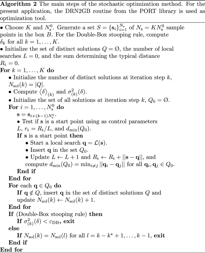
The Double-Box stopping rule can be summarized as follows. Choose the integers K and $N_{\text {s}}^{0}$. Let $B_{2}$ be a larger box that contains B such that $\mu (B_{2})=2\mu (B)$, where $\mu (B)$ is the measure of B. At every iteration k, where $1\le k\le K$, sample $B_{2}$ uniformly until $N_{\text {s}}^{0}$ points fall in B. After k iterations, let $M_{k}$ be the accumulated (total) number of points from $B_{2}$. Then, the quantity $\delta _{k}=kN_{\text {s}}^{0}/M_{k}$ has an expectation value $\bigl \langle \delta \bigr \rangle _{(k)}=(1/k)\sum _{i=1}^{k}\delta _{i}$ that tends to $\mu (B)/\mu (B_{2})=1/2$ as $k\rightarrow \infty$, while the variance $\sigma _{(k)}^{2}(\delta )=(1/k)\sum _{i=1}^{k}(\delta _{i}-\bigl \langle \delta \bigr \rangle _{(k)})^{2}$ tends to zero as $k\rightarrow \infty$. The variance is a smoother quantity than the expectation and is better suited for a termination criterion. Actually, the iterative process is stopped when the variance $\sigma _{(k)}^{2}(\delta )$ is below a prescribed tolerance.

From the above discussion, it is apparent that the Double-Box stopping rule requires a specific sampling. In order to implement all sampling methods into a common framework, we generate a set $S=\{{\mathbf {s}}_{i}\}_{i=1}^{N_{\text {s}}}$ of $N_{\text {s}}=KN_{\text {s}}^{0}$ sample points in the box B, where K is the number of disjoint subsets in which the set S is split, i.e., $S=\cup _{k=1}^{K}S_{k}$, and $N_{\text {s}}^{0}$ the number of sample points in each subset $S_{k}$. Because in some applications, the requirement of finding as many solutions as possible asks for a very small tolerance of the Double-Box stopping rule (and so, for a large number of iterations), we use an alternative termination criterion: If the number of solutions $N_{\text {sol}}(k)$ does not change within $k^{\star }\le K$ iteration steps, i.e., $N_{\text {sol}}(k)=N_{\text {sol}}(l)$ for all $l=k-k^{\star }+1,\ldots ,k-1$, the algorithm stops. Algorithm 2 illustrates the main steps of the stochastic optimization method used in this work.

4 Testing solutions

In the post-processing step, it is straightforward to check

• 1. if for any configuration ${\mathbf {q}}=({\mathbf {q}}_{1}^{T},...,{\mathbf {q}}_{n}^{T})^{T}$, the center of mass of the configuration is located at the vertex (0, 0), that is, if the condition $\sum _{i=1}^{n}m_{i}{\mathbf {q}}_{i}=\varvec{0}$ is satisfied,

• 2. if for any configuration ${\mathbf {q}}=({\mathbf {q}}_{1}^{T},...,{\mathbf {q}}_{n}^{T})^{T}$, the ${\mathbf {S}}$-weighted moment of inertia is normalized to one, that is, if the condition $\sum _{j=1}^{n}m_{j}{\mathbf {q}}_{j}^{T}{\mathbf {S}}{\mathbf {q}}_{j}=1$ is satisfied, and

  

• 3. if for any central configuration ${\mathbf {q}}=({\mathbf {q}}_{1}^{T},...,{\mathbf {q}}_{n}^{T})^{T}$, the residual of the Albouy–Chenciner equations defined as

  $$\begin{aligned} \Delta =\sqrt{\sum _{1\le i<j\le n}f_{ij}^{2}({\mathbf {R}})}, \end{aligned}$$

  where (cf. Eq. 8)

  $$\begin{aligned} f_{ij}({\mathbf {R}})=m\sum _{k=1}^{n}[S_{ik}(R_{jk}^{2}-R_{ik}^{2}-R_{ij}^{2})+S_{jk}(R_{ik}^{2}-R_{jk}^{2}-R_{ij}^{2})],\,\,\,1\le i<j\le n \end{aligned}$$

  and $R_{ij}=||{\mathbf {q}}_{i}-{\mathbf {q}}_{j}||$, is sufficiently small.

Two additional tests related to the fulfillment of the Morse equality and the uniqueness of the solutions are listed below.

4.1 Morse equality

A drawback of the algorithm is that there is no guarantee that in a finite number of steps, all solutions are found. Some hope that the set Q, at least for small n, is complete, that comes from the Morse equality: If ${\widehat{U}}_{n}:{\mathcal {N}}(S)/\text {SO}(2)\rightarrow {\mathbb {R}}$ is a Morse function, we have

$$\begin{aligned} \sum _{k}(-1)^{k}\nu _{k}=\chi ({\mathcal {N}}(S)/\text {SO}(2))=(-1)^{n}(n-2)!, \end{aligned}$$

(20)

where $\nu _{k}$ are the number of critical points of index k and $\chi ({\mathcal {N}}(S)/\text {SO}(2))$ is the Euler characteristic of ${\mathcal {N}}(S)/\text {SO}(2)$ (Ferrario 2002). Each central configuration ${\mathbf {q}}=({\mathbf {q}}_{1}^{T},...,{\mathbf {q}}_{n}^{T})^{T}$ gives rise to central configurations $({\mathbf {q}}_{\sigma (1)}^{T},...,{\mathbf {q}}_{\sigma (n)}^{T})^{T}$ for all $\sigma \in S_{n}$, where $S_{n}$ is the group of permutations of n elements. When the configuration has an axis of symmetry, there are $n!/j({\mathbf {q}})$ many distinct critical points, where $j({\mathbf {q}})$ is the size of the isotropy group of the central configuration ${\mathbf {q}}$. Otherwise, when the configuration has no axis of symmetry, there are $n!/j({\mathbf {q}})$ many distinct critical points, as well as their reflections with respect to an axis in the plane; hence, there are $2n!/j({\mathbf {q}})$ distinct critical points. Let $i({\mathbf {q}})=j({\mathbf {q}})$ when ${\mathbf {q}}$ has an axis of symmetry and $i({\mathbf {q}})=j({\mathbf {q}})/2$ when ${\mathbf {q}}$ has no axis of symmetry. Furthermore, let $h({\mathbf {q}})$ be the Morse index of ${\mathbf {q}}$. Then, for central configurations, the Morse equality (20) becomes

$$\begin{aligned} \sum _{i=1}^{N_{\text {sol}}}\frac{(-1)^{h({\mathbf {q}}_{i})}}{i({\mathbf {q}}_{i})}=\frac{(-1)^{n}}{n(n-1)}. \end{aligned}$$

(21)

The quantities in Eq. (21) are computed as follows.

• 1. For a non-degenerate solution ${\mathbf {q}}$, the Morse index is given by the number of negative eigenvalues of the Hessian matrix (cf. Eq. 7)

  $$\begin{aligned} {\mathbf {H}}({\mathbf {q}})=D^{2}U_{n}({\mathbf {q}})+U_{n}({\mathbf {q}}){\mathbf {S}}{\mathbf {M}}, \end{aligned}$$

  (22)

  where $D^{2}U_{n}({\mathbf {q}})$ is computed as

  $$\begin{aligned} D^{2}U_{n}({\mathbf {q}})&=({\mathbf {D}}_{ij})_{i,j=1}^{n}\in {\mathbb {R}}^{2n\times 2n},\\ {\mathbf {D}}_{ij}&=\frac{m^{2}}{R_{ij}^{3}}({\mathbf {I}}_{2\times 2}-3{\mathbf {u}}_{ij}{\mathbf {u}}_{ij}^{T})\in {\mathbb {R}}^{2\times 2},\,\,\,i\ne j,\\ {\mathbf {D}}_{ii}&=-\sum _{\begin{array}{c} j=1\\ j\not =i \end{array} }^{n}{\mathbf {D}}_{ij},\\ {\mathbf {u}}_{ij}&=({\mathbf {q}}_{i}-{\mathbf {q}}_{j})/R_{ij}. \end{aligned}$$

• 2. The isotropy index is computed as in Ferrario (2002): We count all configurations that are $\text {O}(2)$ invariant; that is, for a configuration ${\mathbf {q}},$ we compute the isotropy index $i({\mathbf {q}})$. Specifically, for any collinear configuration, we take $i({\mathbf {q}})=2$, while for any non-collinear configuration, we take into account that this type of configuration can have (1) as isotropy subgroup, a dihedral group or the cyclic group of order 2, in which case $i({\mathbf {q}})$ is the number of reflection lines of polar angle $\alpha _{0}$ (with $0\le \alpha _{0}<180^{circ}$), or (2) no reflection axis, in which case $i({\mathbf {q}})=1/2$, i.e., the configuration contributes to the sum in Eq. (21) twice. A reflection line can be (1) a ray passing through the vertex at (0, 0) and a point mass or (2) the bisector of the angle with the vertex at (0, 0) and the rays passing through two neighboring points.

4.2 Uniqueness of the solutions

To test if in a small neighborhood of each numerical solution there is a unique exact solution, we use an approach based on the Krawczyk operator method (Lee and Santoprete 2009; Moczurad and Zgliczynski 2019, 2020). This approach, that works hand in hand with the optimization method used, is summarized below.

Consider an overdetermined system of nonlinear equations ${\mathbf {f}}({\mathbf {q}})=\varvec{0}$ with ${\mathbf {q}}\in {\mathbb {R}}^{N}$, ${\mathbf {f}}({\mathbf {q}})=(f_{1}({\mathbf {q}}),f_{2}({\mathbf {q}}),\ldots ,f_{M}({\mathbf {q}}))^{T}\in {\mathbb {R}}^{M}$, $M\ge N$, and the objective function $F({\mathbf {q}})=(1/2)||{\mathbf {f}}({\mathbf {q}})||^{2}$. In the Gauss–Newton method for solving the least-squares problem $\min _{{\mathbf {q}}}F({\mathbf {q}})$, the search direction ${\mathbf {p}}_{k}={\mathbf {q}}_{k+1}-{\mathbf {q}}_{k}$ satisfies the equation ${\mathbf {J}}_{f}^{T}({\mathbf {q}}_{k}){\mathbf {J}}_{f}({\mathbf {q}}_{k}){\mathbf {p}}=-{\mathbf {J}}_{f}^{T}({\mathbf {q}}_{k}){\mathbf {f}}({\mathbf {q}}_{k})$, where ${\mathbf {J}}_{f}({\mathbf {q}})=D{\mathbf {f}}({\mathbf {q}})\in {\mathbb {R}}^{M\times N}$ is the Jacobian matrix of ${\mathbf {f}}$. In other words, the new iterate is computed as

$$\begin{aligned} {\mathbf {q}}_{k+1}={\mathbf {q}}_{k}-[{\mathbf {J}}_{f}^{T}({\mathbf {q}}_{k}){\mathbf {J}}_{f}({\mathbf {q}}_{k})]^{-1}{\mathbf {J}}_{f}^{T}({\mathbf {q}}_{k}){\mathbf {f}}({\mathbf {q}}_{k}). \end{aligned}$$

(23)

An equivalent interpretation of the iteration formula (23) can be given by taking into account that the gradient and the Gauss–Newton approximation to the Hessian of $F({\mathbf {q}})$ are given by ${\mathbf {g}}({\mathbf {q}})=DF({\mathbf {q}})={\mathbf {J}}_{f}^{T}({\mathbf {q}}){\mathbf {f}}({\mathbf {q}})$ and ${\mathbf {J}}_{g}({\mathbf {q}})=D{\mathbf {g}}({\mathbf {q}})=D^{2}F({\mathbf {q}})\approx {\mathbf {J}}_{f}^{T}({\mathbf {q}}){\mathbf {J}}_{f}({\mathbf {q}})$, respectively. The first-order necessary condition for optimality requires that ${\mathbf {g}}({\mathbf {q}})=0$. If this equation is solved by means of the Newton method we are led to the iteration formula

$$\begin{aligned} {\mathbf {q}}_{k+1}={\mathbf {q}}_{k}-[{\mathbf {J}}_{g}({\mathbf {q}}_{k})]^{-1}{\mathbf {g}}({\mathbf {q}}_{k}), \end{aligned}$$

(24)

which coincides with that given by Eq. (23). In order to test the uniqueness, we use the interval arithmetic library INTLIB (Kearfott et al. 1994), and let $[{\mathbf {q}}]_{r}\subset {\mathbb {R}}^{N}$ be an interval set centered at a numerical solution ${\mathbf {q}}$ with radius r sufficiently small (e.g., $r=10^{-8}$). The procedure involves two steps.

• Step 1. Check if global minima of F exist in $[{\mathbf {q}}]_{r}$, that is, if ${\mathbf {0}}\in {\mathbf {f}}([{\mathbf {q}}]_{r})$.

• Step 2. Check if there exists a unique stationary point of F in $[{\mathbf {q}}]_{r}$, that is, if there exists a unique zero of the first-order optimality equation ${\mathbf {g}}({\mathbf {q}})=0$. For this purpose, we define the Krawczyk operator by

  $$\begin{aligned} K({\mathbf {q}},[{\mathbf {q}}]_{r},{\mathbf {g}})={\mathbf {q}}-{\mathbf {C}}{\mathbf {g}}({\mathbf {q}})+[{\mathbf {I}}_{N\times N}-{\mathbf {C}}{\mathbf {J}}_{g}([{\mathbf {q}}]_{r})]([{\mathbf {q}}]_{r}-{\mathbf {q}}), \end{aligned}$$

where ${\mathbf {C}}\in {\mathbb {R}}^{N\times N}$ is a preconditioning matrix which is sufficiently close to $[{\mathbf {J}}_{g}({\mathbf {q}})]^{-1}$, and ${\mathbf {I}}_{N\times N}$ is the identity matrix. A property of the Krawczyk operator, which provides a method for proving the existence of a unique zero in a given interval set, states that if $K({\mathbf {q}},[{\mathbf {q}}]_{r},{\mathbf {g}})\subset \text {int}[{\mathbf {q}}]_{r}$, then there exists a unique zero of ${\mathbf {g}}$ in $[{\mathbf {q}}]_{r}$. Following the recommendations of Kearfoot (1996), the computational process is organized as follows:

• 1. compute the matrices $m({\mathbf {J}}_{g}([{\mathbf {q}}]_{r})$ and $\Delta {\mathbf {J}}_{g}([{\mathbf {q}}]_{r})$ according to the decomposition ${\mathbf {J}}_{g}([{\mathbf {q}}]_{r})=m({\mathbf {J}}_{g}([{\mathbf {q}}]_{r})+\Delta {\mathbf {J}}_{g}([{\mathbf {q}}]_{r})$, where $m({\mathbf {J}}_{g}([{\mathbf {q}}]_{r})$ is the center matrix of the interval matrix ${\mathbf {J}}_{g}([{\mathbf {q}}]_{r})$ (the center matrix of an interval matrix is defined componentwise according to the rule $m([\underline{x},\overline{x}])=(\underline{x}+\overline{x})/2$);

• 2. choose the preconditioning matrix ${\mathbf {C}}$ as the inverse of $m({\mathbf {J}}_{g}([{\mathbf {q}}]_{r})$, that is, ${\mathbf {C}}=[m({\mathbf {J}}_{g}([{\mathbf {q}}]_{r})]^{-1}$;

• 3. to account for rounding errors in the calculation of ${\mathbf {g}}({\mathbf {q}})$, compute instead ${\mathbf {g}}([{\mathbf {q}}]_{r})$ by using interval arithmetic;

• 4. calculate $K({\mathbf {q}},[{\mathbf {q}}]_{r},{\mathbf {g}})$ by means of the relation

  $$\begin{aligned} K({\mathbf {q}},[{\mathbf {q}}]_{r},{\mathbf {g}})={\mathbf {q}}-{\mathbf {C}}{\mathbf {g}}([{\mathbf {q}}]_{r})-{\mathbf {C}}\,\Delta {\mathbf {J}}_{g}([{\mathbf {q}}]_{r})([{\mathbf {q}}]_{r}-{\mathbf {q}}). \end{aligned}$$

Because any global minimum satisfies the first-order optimality condition, we infer that if both conditions ${\mathbf {0}}\in {\mathbf {f}}([{\mathbf {q}}]_{r})$ and $K({\mathbf {q}},[{\mathbf {q}}]_{r},{\mathbf {g}})\subset \text {int}[{\mathbf {q}}]_{r}$ are satisfied, then there exists a unique global minimum of F in $[{\mathbf {q}}]_{r}$, and so, a unique solution of the system of nonlinear equations ${\mathbf {f}}({\mathbf {q}})=\varvec{0}$ in $[{\mathbf {q}}]_{r}$.

For balanced configurations, the test is used with $M=N=2n$ and ${\mathbf {f}}({\mathbf {q}})=(f_{1}({\mathbf {q}}),f_{2}({\mathbf {q}}),\ldots ,f_{N}({\mathbf {q}}))^{T},$ where $f_{2i-1}({\mathbf {q}})$ and $f_{2i}({\mathbf {q}})$, $i=1,\ldots ,n$ are given by Eqs. (12) and (13), respectively. For central configurations, we have to consider a system of nonlinear equations, in which continuous rotations are eliminated. This is accomplished, by rotating the configuration ${\mathbf {q}}$ such that the point mass with the maximum radial distance is on the x-axis. Let $i_{0}$ be the index of this point mass and ${\mathbf {q}}^{\prime }$ the rotated configuration. In addition to the functions $f_{2i-1}({\mathbf {q}})$ and $f_{2i}({\mathbf {q}})$, $i=1,\ldots ,n$, we include the constraint

$$\begin{aligned} f_{2n+1}({\mathbf {q}})=y_{i_{0}} \end{aligned}$$

(25)

in the objective function $F({\mathbf {q}})$ and apply the above test in the case $M=2n+1>N=2n$ for the interval set $[{\mathbf {q}}^{\prime }]_{r}\subset {\mathbb {R}}^{N}$ centered at the rotated solution ${\mathbf {q}}^{\prime }$.

Another option for checking the uniqueness is to perform a random test. If the solution ${\mathbf {q}}\in Q$ is a unique global minimum of F, that is, if (1) the gradient of F vanishes at ${\mathbf {q}}$, and (2) the Hessian of F is positive definite at ${\mathbf {q}}$, then the quadratic approximation

$$\begin{aligned} F({\mathbf {p}}_{i})\approx \frac{1}{2}({\mathbf {p}}_{i}-{\mathbf {q}})^{T}D^{2}F({\mathbf {q}})({\mathbf {p}}_{i}-{\mathbf {q}}) \end{aligned}$$

(26)

should be valid at a set of sample points $\{{\mathbf {p}}_{i}\}_{i=1}^{N_{\mathrm {q}}}\subset [{\mathbf {q}}]_{r}$ with r sufficiently small (e.g., $r=10^{-3}||{\mathbf {q}}||$). As before, we use the Gauss–Newton approximation to the Hessian matrix, i.e., $D^{2}F({\mathbf {q}})\approx {\mathbf {J}}_{f}^{T}({\mathbf {q}}){\mathbf {J}}_{f}({\mathbf {q}})$, and generate $N_{\mathrm {q}}=10^{4}$ sample points ${\mathbf {p}}_{i}$ by using a pseudo-random number generator. For central configurations, we either eliminate a sample ${\mathbf {p}}$ if it is a rotated version of ${\mathbf {q}}$ or, as before, include the constraint $f_{2n+1}({\mathbf {q}})=y_{i_{0}}$ in the objective function $F({\mathbf {q}})$. In practice, we test if the RMS of the relative quadratic approximation errors

$$\begin{aligned} \text {RMS}({\mathbf {q}})=\sqrt{\frac{\sum _{i=1}^{N_{\mathrm {q}}}\varepsilon ({\mathbf {q}},{\mathbf {p}}_{i})^{2}}{N_{\mathrm {q}}},} \end{aligned}$$

(27)

where (cf. Eq. 26)

$$\begin{aligned} \varepsilon ({\mathbf {q}},{\mathbf {p}}_{i})=\frac{F({\mathbf {p}}_{i})-\frac{1}{2}||{\mathbf {J}}_{f}({\mathbf {q}})({\mathbf {p}}_{i}-{\mathbf {q}})||^{2}}{F({\mathbf {p}}_{i})} \end{aligned}$$

for $i=1,\ldots ,N_{\mathrm {q}}$, is below a prescribed tolerance.

Table 1 The number of central configurations $N_{\text {sol}}$

Fig. 1

The three central configurations that complete the list of Ferrario (2002). Note that Configurations 2 and 3 do not coincide with the regular decagon. Moreover, they are very similar but not identical; the radial distances are slightly different and when they are aligned with the maximum radial distance along the x-axis, Configuration 2 has (only) the axes of symmetry $\alpha _{1}=72^\circ$ and $\alpha _{2}=162^\circ ,$ while Configuration 3 has the axes of symmetry $\alpha =0^\circ$ and $\alpha _{2}=90^\circ$

Table 2 The number of balanced configurations $N_{\text {sol}}$ for $n=5$ masses

Fig. 2

Balanced configurations for five masses in the case $\sigma _{x}=1.0$ and $\sigma _{y}=0.1$. The $x_{i}$ and $y_{i}$ coordinates are normalized according to the rules: $x_{i}\rightarrow \sqrt{m\sigma _{x}}x_{i}$ and $y_{i}\rightarrow \sqrt{m\sigma _{y}}y_{i}$, respectively

Fig. 3

The same as in Fig. 2 but for $\sigma _{y}=0.2$

Fig. 4

The same as in Fig. 2 but for $\sigma _{y}=0.3$

Fig. 5

The same as in Fig. 2 but for $\sigma _{y}=0.4$.(continued on next page)

Fig. 6

The same as in Fig. 2 but for $\sigma _{y}=0.5$

Fig. 7

The same as in Fig. 2 but for $\sigma _{y}=0.6$

Fig. 8

The same as in Fig. 2 but for $\sigma _{y}=0.7$

Fig. 9

The same as in Fig. 2 but for $\sigma _{y}=0.8$

Fig. 10

Central configurations ($\sigma _{x}=\sigma _{y}=1.0$) for five masses. The $x_{i}$ and $y_{i}$ coordinates are normalized as in Fig. 2

Fig. 11

Balanced configurations for four equal masses without any axis of symmetry. They seem to be centrally symmetric. In these simulations, $\sigma _{x}=1.0$ and $\sigma _{y}$ is increased from 0.25 (panel 1) to 0.33 (panel 9) in steps of 0.01

Fig. 12

Some balanced configurations without any symmetry for ten masses in the case $\sigma _{x}=1.0$ and $\sigma _{y}=0.3$

5 Numerical results

The performances of the algorithm, and in particular, the number of numerical solutions found, depend on the selection of a set of control parameters. These are chosen as follows.

• 1. The configuration ${\mathbf {q}}$ is considered to be an approximate solution to the optimization problem, if $F({\mathbf {q}})<10^{-20}$.

• 2. The set of distinct solutions Q contains only non-degenerate solutions. If $\lambda _{i}$ are the eigenvalues of the Hessian matrix (22) sorted in ascending order, i.e., $|\lambda _{1}|\le |\lambda _{2}|\le \ldots \le |\lambda _{2n}|$, the central configuration ${\mathbf {q}}$ is assumed to be an approximate degenerate solution if $|\lambda _{2}({\mathbf {q}})|<10^{-15}$, while for balanced configurations, the criterion is $|\lambda _{1}({\mathbf {q}})|<10^{-15}$. In this context, the Morse index of a central configuration ${\mathbf {q}}$ is given by the number of negative eigenvalues $\lambda _{i}$ of the Hessian matrix for all $i\ge 2$.

• 3. The ordered sets of mutual distances $R_{ij}=||{\mathbf {q}}_{i}-{\mathbf {q}}_{j}||$ and $R_{ij}^{\prime }=||{\mathbf {q}}_{i}^{\prime }-{\mathbf {q}}_{j}^{\prime }||$ corresponding to the configurations ${\mathbf {q}}=({\mathbf {q}}_{1}^{T},...,{\mathbf {q}}_{n}^{T})^{T}$ and ${\mathbf {q}}^{\prime }=({\mathbf {q}}_{1}^{\prime T},...,{\mathbf {q}}_{n}^{\prime T})^{T}$, respectively, are considered to be approximately identical if $|R_{ij}-R_{ij}^{\prime }|\le 10^{-6}[1+\max (|R_{ij}|,|R_{ij}^{\prime })]$ for all $1\le i<j\le n$.

The results of our numerical analysis are available at the website: https://github.com/AlexandruDoicu/Balanced-and-Central-Configurations. The simulations were performed on a computer Intel Core i5-3340M CPU 2.70GHz with 8 GB RAM. The output file for each balanced configuration contains: (1) the value of the objective function, (2) the Cartesian coordinates of the point masses, (3) the residual of the normalization condition for the moment of inertia, (4) the Cartesian coordinates of the center of mass, (5) the RMS of the relative quadratic approximation error and the maximum quadratic approximation error, (6) a logical flag indicating if global minima of F exist in a small box around the solution, as well as, a logical flag indicating if there is a unique stationary point of F in the same box, and (7) the number of degenerate solutions and the corresponding Cartesian coordinates of the point masses. For central configurations, the output file contains in addition (1) the residual of the Albouy–Chenciner equations, (2) the Morse and isotropy indices, and (3) the residual of the Morse equation.

For $n\le 12$, the existence and local uniqueness of any central configuration were independently tested by Moczurad and Zgliczynski using their code based on the Krawczyk operator method (Moczurad and Zgliczynski 2019).

5.1 Central configurations

The number of central configurations for $m=0.1$ and $\sigma _{x}=\sigma _{y}=1.0$ is listed in Table 1. The results correspond to a number of masses n ranging from 3 to 12. The following comments can be made here.

• 1. In all cases, the Morse equality (21) is satisfied, the conditions ${\mathbf {0}}\in {\mathbf {f}}([{\mathbf {q}}]_{r})$ and $K({\mathbf {q}},[{\mathbf {q}}]_{r},{\mathbf {g}})\subset \text {int}[{\mathbf {q}}]_{r}$ are fulfilled, and the RMS of the relative quadratic approximation errors (27) is smaller than $2\times 10^{-4}$.

• 2. For $n\le 10$, all tested sampling methods (Double-Box, Chaotic, Faure, Sobol, Latin Hypercube, and Quasi-Oppositional Differential Evolution) yield the same results. For $n=11$, only a Chaotic Method leads to a set of central configurations for which the Morse equality is satisfied, while for $n=12$ both a Chaotic Method and a Faure sequence fulfill this desire. The case $n=11$, requiring large values for $N_{\text {s}}^{0}$, K, and $k^{\star }$, is the most challenging.

• 3. A Chaotic Method followed by a Faure sequence is the most efficient. The reason is that the sets of starting points are much smaller than the sets corresponding to other sampling methods.

• 4. All central configurations corresponding to $n\le 9$ are identical to those presented in Ferrario (2002). In this work, only 64 central configurations that do not satisfy the Morse equality have been found in the case $n=10$. The remaining configurations are illustrated in Fig. 1.

• 5. As compared to other solvers described in the literature (Lee and Santoprete 2009; Moczurad and Zgliczynski 2019), the stochastic optimization algorithm is extremely efficient. However, it should be pointed out that the methods used in Moczurad and Zgliczynski (2019), and Lee and Santoprete (2009) are rigorous, in the sense that the complete list of central configurations is provided; in our approach, there is no guarantee that the list is complete.

5.2 Balanced configurations

The number of balanced configurations for five identical masses $m=1$ is listed in Table 2, while the corresponding configurations are illustrated in Figs. 2,  3, 4, 5, 6, 7, 8, and 9. The sampling method was a Faure sequence. In these simulations, we took $\sigma _{x}=1.0$ and changed $\sigma _{y}$ from 0.1 to 0.8 in steps of 0.1. Thus, the ratio $\sigma _{y}/\sigma _{x}$ varies from 0.1 to 0.8. For a comparison, the central configuration ($\sigma _{x}=\sigma _{y}=1.0)$ for five masses is shown in Fig. 10. From our numerical analysis, the following conclusions can be drawn:

• 1. In all cases, the collinear configurations along the x- and y-axis are present. Moreover, the collinear configurations along the x-axis are identical (as they should).

• 2. Some configuration shapes appear in all test examples. This result suggests that the balanced configurations can be classified according to the similarity of their shapes.

• 3. The shapes of the central configurations are also similar with, for example, the shapes of the balanced configurations in the case $\sigma _{y}=0.8$. (The shapes (1), (2), (3), (4), and (5) are similar to the shapes (10), (7), (2), (5), and (9), respectively.)

For $n<8$, all central configurations have at least one axis of symmetry. Although we did not perform an exhaustive numerical analysis, we make some preliminary comments related to balanced configurations without any axis of symmetry.

• 1. In Chenciner (2017), it was asked whether in the case $n=4$, balanced configurations without any axis of symmetry exist. Through a numerical analysis, we found that for $\sigma _{x}=1.0$ and some specific values of $\sigma _{y}$, such balanced configurations exist (Fig. 11). These results together with those corresponding to $\sigma _{x}=1.0$ and $\sigma _{y}$ ranging from 0.1 to 0.8 in steps of 0.1 are provided at website https://github.com/AlexandruDoicu/Balanced-and-Central-Configurations.

• 2. In the case $n=5$, examples of balanced configurations without any axis of symmetry are: (4) in Fig. 4 for $\sigma _{y}=0.3$, and (4) and (10) in Fig. 5 for $\sigma _{y}=0.4$.

• 3. In the case $n=10$, there are 67 central configurations from which 11 are without any axis of symmetry. For the same number of point masses, there are much more balanced configurations, and accordingly, much more asymmetrical configurations. As an example, we mention that for $n=10$, $\sigma _{x}=1.0$ and $\sigma _{y}=0.3$, we found 270 balanced configurations from which 90 are without any axis of symmetry. Some examples are illustrated in Fig. 12. Note that these results were computed by using a Chaotic Method and the control parameters $N_{\text {s}}^{0}=K=2000$ and $k^{\star }=500$; the computational time was 59 minutes and 45 seconds.

6 Conclusions

A stochastic optimization algorithm for analyzing planar central and balanced configurations in the n-body problem has been developed. The algorithm has been designed around the Minfinder method developed by Tsoulos et al. (2006) by including additional sampling and local optimization methods. In the post-processing stage, several solution tests have been incorporated. These are related to the fulfillment of the normalization condition for the moment of inertia, the Albouy–Chenciner equations, the Morse equality, and the uniqueness of the solutions. Through a numerical analysis, we found an extensive list of central configurations satisfying the Morse equality up to $n=12$. However, based on a random search, the algorithm is able to find the complete list of central configurations (at least for $n\le 9$) with a low computational time cost. For balanced configurations, we showed some exemplary results in the case $n=5$, and some configurations without any axis of symmetry in the cases $n=4$ and $n=10$.

The developed algorithm is versatile and has a wide range of application. In addition to the Cartesian coordinates $(x_{i},y_{i})$, the masses $m_{i}$ and the standard deviations $\sigma _{x}$ and $\sigma _{y}$ can be included in the inversion process. Actually, the unknown vector ${\mathbf {q}}$ is defined as

$$\begin{aligned} {\mathbf {q}}=[(x_{1},y_{1}),\ldots ,(x_{n},y_{n}),m_{1},\ldots ,m_{n},\sigma _{x},\sigma _{y}]^{T}, \end{aligned}$$

and a logical array specifies which components of the vector are considered in the optimization process. Moreover, the algorithm can be directly extended to spatial configurations and additional types of constraints, similar to that given by Eq. (25), can be taken into account. With these enhancements, the algorithm can be used, for example, to analyze n-body central configurations with a homogeneous potential (Hampton 2019), to compute the central configurations for the n-body problem by solving the Albouy–Chenciner equations, to determine the central configurations for the $(n+1)$-body problem or the so-called super central configurations (Xie (2010)) for the n-body problem.

References

Albouy, A., Chenciner, A.: Le problème des \(N\) corps et les distances mutuelles. Invent. Math. 131, 151–184 (1998)
Albouy, A., Kaloshin, V.: Finiteness of central configurations of five bodies in the plane. Ann. Math. 176, 535–588 (2012)
Ali, M.M., Storey, C.: Topographical multilevel single linkage. J. Global Optim. 5, 349–358 (1994)
Becker, R.W., Lago, G.V.: A global optimization algorithm. In: Proceedings of the 8th Allerton Conference on Circuits and Systems Theory (1970)
Boender, C.G.E., Kan, A.H.G.R., Timmer, G.T., Stougie, L.: A stochastic method for global optimization. Math. Program. 22, 125–140 (1982)
Boender, C.G.E., Kan, A.H.G.R.: Bayesian stopping rules for multistart global optimization methods. Math. Program. 37, 59–80 (1987)
Boender, C.G.E., Romeijn, H.E.: Stochastic methods. In: Horst, R., Pardalos, P.M. (eds.) Handbook of Global Optimization, pp. 829–871. Kluwer, Dordrecht (1995)
Byrd, R.H., Lu, P., Nocedal, J., Zhu, C.: A limited memory algorithm for bound constrained optimization. SIAM J. Sci. Comput. 16, 1190–1208 (1995)
Chenciner, A.: Are nonsymmetric balanced configurations of four equal masses virtual or real? Regul. Chaot. Dyn. 22, 677–687 (2017)
Dennis, J.E., Jr., Gay, D.M., Welsch, R.E.: An adaptive nonlinear least-squares algorithm. ACM Trans. Math. Softw. 7, 348–368 (1981)
Dennis Jr., J.E., Gay D.M., Welsch R.E.: Algorithm 573. NL2SOL—An adaptive nonlinear least-squares algorithm. ACM Trans. Math. Softw. 7, 369–383 (1981)
Dong, N., Wu, C.-H., Ip, W.-H., Chen, Z.-Q., Chan, C.-Y., Yung, K.-L.: An opposition-based chaotic ga/pso hybrid algorithm and its application in circle detection. Comput. Math. with Appl. 64, 1886–1902 (2012)
Du, Q., Gunzburger, M., Ju, L.: Advances in studies and applications of centroidal Voronoi tessellations. Numer. Math. Theory Methods Appl. 3, 119–142 (2010)
Euler, L.: De motu rectilineo trium corporum se mutuo attrahentium, Novi Comm. Acad. Sci. Imp. Petrop. 11, 144–151 (1767)
Ferrario, D.: Central configurations, symmetries and fixed points. arXiv:math/0204198v1 (2002)
Fletcher, R.: A new approach to variable metric algorithms. Comput. J. 13, 317–322 (1970)
Gao, Y., Wang, Y.-J.: A memetic differential evolutionary algorithm for high dimensional functions optimization. In: Third International Conference on Natural Computation (ICNC 2007), vol. 4, pp. 188–192. IEEE (2007)
Gao, W.-F., Liu, S.-Y.: A modified artificial bee colony algorithm. Comput. Oper. Res. 39, 687–697 (2012)
Hampton, M.: Planar \(N-\)body central configurations with a homogeneous potential. Celest. Mech. Dyn. Astr. 131, 20 (2019). https://doi.org/10.1007/s10569-019-9898-0
Hampton, M., Jensen, A.: Finiteness of spatial central configurations in the five-body problem. Celest. Mech. Dyn. Astr. 109, 321–332 (2011). https://doi.org/10.1007/s10569-010-9328-9
Hampton, M., Moeckel, R.: Finiteness of relative equilibria of the four-body problem. Invent. Math. 163, 289–312 (2006)
Hanson, R.J., Krogh, F.T.: A quadratic-tensor model algorithm for nonlinear least-squares problems with linear constraints. ACM Trans. Math. Softw. 18, 115–133 (1992)
Kearfoot, R.B.: Rigorous Global Search: Continuous Problems. Kluwer, Dordrecht (1996)
Kearfott, R.B., Dawande, M., Du, K., Hu, C.: Algorithm 737: INTLIB—a portable Fortran 77 interval standard-function library. ACM Trans. Math. Softw. (1994). https://doi.org/10.1145/198429.198433
Lagaris, I.E., Tsoulos, I.G.: Stopping rules for box-constrained stochastic global optimization. Appl. Math. Comput. 197, 622–632 (2008)
Lagrange, J.L.: Essai sur le probléme des trois corps, Oeuvres, vol. 6 (1772)
Lee, T.-L., Santoprete, M.: Central configurations of the five-body problem with equal masses. arXiv:0906.0148v1 (2009)
Marsaglia, G., Tsang, W.W.: The Ziggurat method for generating random variables. J. Stat. Softw. 5, 8 (2000)
Matsumoto, M., Nishimura, T.: Mersenne twister: a 623-dimensionally equidistributed uniform pseudorandom number generator. ACM Trans. Model. Comput. Simul. 1, 3–30 (1998)
McKay, M.D., Beckman, R.J., Conover, W.J.: A comparison of three methods for selecting values of input variables in the analysis of output from a computer code. Technometrics 21, 239–245 (1979)
Moczurad, M., Zgliczynski, P.: Central configurations in planar \(n\)-body problem with equal masses for \(n=5,6,7\). Celest. Mech. Dyn. Astron. 131, 46 (2019)
Moczurad, M., Zgliczynski, P.: Central configurations in spatial \(n\)-body problem for \(n=5,6\) with equal masses. arXiv:2006.06768 (2020)
Moeckel, R.: Some relative equilibria on \(N\) equal masses, \(N=4,5,6,7\). http://www-users.math.umn.edu/~rmoeckel/research/CC.pdf (1989). Accessed 2 Aug 2020
Moeckel, R.: Generic finiteness for Dziobek configurations. Trans. Am. Math. Soc. 353(11), 4673–4686 (2001)
Moeckel, R.: Lectures On Central Configurations. http://www-users.math.umn.edu/rmoeckel/notes/CentralConfigurations.pdf (2014a)
Moeckel, R.: Central configurations. Scholarpedia 9(4), 10667 (2014b). https://doi.org/10.4249/scholarpedia.10667
More, J.J., Wright, S.J.: Optimization Software Guide. SIAM, Philadelphia (1993)
Powel, M.J.D.: A tolerant algorithm for linearly constrained optimization calculations. Math. Program. 45, 547 (1989)
Rahnamayan, S., Tizhoosh, H.R., Salama, M.M.: Opposition-based differential evolution for optimization of noisy problems. In: 2006 IEEE International Conference on Evolutionary Computation, pp. 1865–1872. IEEE (2006)
Rahnamayan, S., Tizhoosh, H.R., Salama, M.M.: Opposition-based differential evolution. Evol. Comput. 12, 64–79 (2008)
Kan, A.H.G.R., Timmer, G.T.: Stochastic global optimization methods. Part I: clustering methods. Math. Program. 39, 27–56 (1987a)
Kan, A.H.G.R., Timmer, G.T.: Stochastic global optimization methods. Part II: multilevel methods. Math. Program. 39, 57–78 (1987b)
Schnabel, R.B., Frank, P.D.: Tensor methods for nonlinear C equations. SIAM J. Num. Anal. 21, 815–843 (1984)
Shub, M.: Diagonals and relative equilibria, appendix to Smale’s paper. Springer Lecture Notes Mathematics 197, 199–201 (1970)
Smale, S.: Mathematical problems for the next century. Math. Intell. 20, 7–15 (1998)
Törn, A.A.: A search clustering approach to global optimization. In: Dixon, L.C.W., Szegö, G.P. (eds.) Towards Global Optimizations. North-Holland, Amsterdam (1978)
Tsoulos, I.G., Lagaris, I.E.: MinFinder. Locating all the local minima of a function. Comput. Phys. Commun. 174, 166–179 (2006)
Xia, Z.: Central configurations with many small masses. J. Differ. Equ. 91, 168–179 (1991)
Xie, Z.: Super central configurations of the \(n\)-body problem. J. Math. Phys. 51,(2010). https://doi.org/10.1063/1.3345125
Zieliński, R.: A statistical estimate of the structure of multiextremal problems. Math. Program. 21, 348–356 (1981)
Acknowledgements
The authors thank Piotr Zgliczynski and Malgorzata Moczurad for their helpful comments and critics, which bring various improvements of this work, and for the independent verification of our solutions with their code based on the Krawczyk operator method. Alexandru Doicu and Lei Zhao were supported by DFG ZH 605/1-1.
Funding
Open Access funding enabled and organized by Projekt DEAL.
Author information
Authors and Affiliations
Corresponding author
Additional information
Publisher's Note
Springer Nature remains neutral with regard to jurisdictional claims in published maps and institutional affiliations.
Rights and permissions
Open Access This article is licensed under a Creative Commons Attribution 4.0 International License, which permits use, sharing, adaptation, distribution and reproduction in any medium or format, as long as you give appropriate credit to the original author(s) and the source, provide a link to the Creative Commons licence, and indicate if changes were made. The images or other third party material in this article are included in the article’s Creative Commons licence, unless indicated otherwise in a credit line to the material. If material is not included in the article’s Creative Commons licence and your intended use is not permitted by statutory regulation or exceeds the permitted use, you will need to obtain permission directly from the copyright holder. To view a copy of this licence, visit http://creativecommons.org/licenses/by/4.0/.
About this article
Cite this article
Doicu, A., Zhao, L. & Doicu, A. A stochastic optimization algorithm for analyzing planar central and balanced configurations in the n-body problem. Celest Mech Dyn Astron 134, 29 (2022). https://doi.org/10.1007/s10569-022-10075-7
Received:
Revised:
Accepted:
Published:
DOI: https://doi.org/10.1007/s10569-022-10075-7