
Abstract
A machine-learning-based methodology is proposed to delineate the spatial distribution of geomaterials across a large-scale three-dimensional subsurface system. The study area spans the entire Po River Basin in northern Italy. As uncertainty quantification is critical for subsurface characterization, the methodology is specifically designed to provide a quantitative evaluation of prediction uncertainty at each location of the reconstructed domain. The analysis is grounded on a unique dataset that encompasses lithostratigraphic data obtained from diverse sources of information. A hyperparameter selection technique based on a stratified cross-validation procedure is employed to improve model prediction performance. The quality of the results is assessed through validation against pointwise information and available hydrogeological cross-sections. The large-scale patterns identified are in line with the main features highlighted by typical hydrogeological surveys. Reconstruction of prediction uncertainty is consistent with the spatial distribution of available data and model accuracy estimates. It enables one to identify regions where availability of new information could assist in the constraining of uncertainty. The comprehensive dataset provided in this study, complemented by the model-based reconstruction of the subsurface system and the assessment of the associated uncertainty, is relevant from a water resources management and protection perspective. As such, it can be readily employed in the context of groundwater availability and quality studies aimed at identifying the main dynamics and patterns associated with the action of climate drivers in large-scale aquifer systems of the kind here analyzed, while fully embedding model and parametric uncertainties that are tied to the scale of investigation.
Résumé
Une méthodologie basée sur l’apprentissage automatique est proposée pour délimiter la distribution spatiale des matériaux géologiques constitutifs d’un système de subsurface tridimensionnel à grande échelle. La zone d’étude s’étend sur l’ensemble du bassin du Pô, dans le nord de l’Italie. La quantification de l’incertitude étant essentielle pour la caractérisation de la subsurface, la méthodologie est spécifiquement conçue pour fournir une évaluation quantitative de l’incertitude de la prédiction à chaque endroit du domaine reconstruit. L’analyse est fondée sur un ensemble de données unique qui englobe des données lithostratigraphiques obtenues à partir de diverses sources d’information. Une technique de sélection d’hyperparamètres basée sur une procédure de validation croisée stratifiée est utilisée pour améliorer les performances de prédiction du modèle. La qualité des résultats est évaluée par une validation par rapport aux informations ponctuelles et aux coupes transversales hydrogéologiques disponibles. Les schémas à grande échelle identifiés sont conformes aux principales caractéristiques mises en évidence par les études hydrogéologiques spécifiques. La reconstruction de l’incertitude des prévisions est cohérente avec la distribution spatiale des données disponibles et des estimations de la précision du modèle. Elle permet d’identifier les régions où la disponibilité de nouvelles informations pourrait contribuer à limiter l’incertitude. L’ensemble des données fournies dans cette étude, complété par la reconstruction du système souterrain basée sur un modèle et l’évaluation de l’incertitude associée, est pertinent du point de vue de la gestion et de la protection des ressources en eau. En tant que tel, il peut être facilement utilisé dans le contexte d’études sur la disponibilité et la qualité des eaux souterraines visant à identifier les principales dynamiques et les schémas associés à l’action des facteurs climatiques dans les systèmes aquifères à grande échelle comme celui analysé ici, tout en intégrant pleinement les incertitudes du modèle et des paramètres qui sont liées à l’échelle de l’étude.
Resumen
Se propone una metodología basada en el aprendizaje automático para delinear la distribución espacial de los geomateriales en un sistema tridimensional del subsuelo a gran escala. El área de estudio abarca toda la cuenca del río Po en el norte de Italia. Dado que la cuantificación de la incertidumbre es fundamental para la caracterización del subsuelo, la metodología se ha diseñado específicamente para proporcionar una evaluación cuantitativa de la incertidumbre de la predicción en cada ubicación del dominio reconstruido. El análisis se basa en un conjunto de datos único que abarca datos litoestratigráficos obtenidos de diversas fuentes de información. Se emplea una técnica de selección de hiperparámetros basada en un procedimiento de validación cruzada estratificada para mejorar el rendimiento de la predicción del modelo. La calidad de los resultados se evalúa mediante la validación con información puntual y secciones hidrogeológicas transversales disponibles. Los patrones a gran escala identificados coinciden con las principales características destacadas por los estudios hidrogeológicos típicos. La reconstrucción de la incertidumbre de la predicción es coherente con la distribución espacial de los datos disponibles y las estimaciones de precisión del modelo. Permite identificar las regiones en las que la disponibilidad de nueva información podría ayudar a limitar la incertidumbre. El amplio conjunto de datos proporcionado en este estudio, complementado por la reconstrucción basada en modelos del sistema del subsuelo y la evaluación de la incertidumbre asociada, es relevante desde una perspectiva de gestión y protección de los recursos hídricos. Como tal, puede emplearse fácilmente en el contexto de los estudios de disponibilidad y calidad de las aguas subterráneas destinados a identificar las principales dinámicas y patrones asociados a la acción de los factores climáticos en sistemas acuíferos a gran escala como los aquí analizados, integrando al mismo tiempo las incertidumbres paramétricas y del modelo vinculadas a la escala de investigación.
摘要
提出了一种基于机器学习的方法, 用于刻画大尺度三维地下水系统中地质介质的空间分布。研究区域跨越意大利北部的整个Po河流域。由于不确定性量化对于地下特征的刻画至关重要, 该方法专门设计用于在重建区的每个位置提供预测不确定性的定量评估。该分析基于一个独特的数据集, 包括来自不同信息源获得的岩性地层数据。采用基于分层交叉验证程序的超参数选择技术, 以提高模型的预测性能。通过与点信息和可用的水文地质剖面进行了验证, 评估了结果的质量。所确定的大尺度模式与典型水文地质调查所强调的主要特征一致。预测不确定性的重构与可用数据的空间分布和模型准确性估计一致。它使我们能够确定利用新信息可帮助约束不确定性的区域。本研究提供的综合数据集, 结合基于模型的地下水系统重建和相关不确定性的评估, 从水资源管理和保护的角度具有重要意义。因此, 它可以容易应用于研究地下水资源可用性和质量, 旨在识别与气候驱动因素在这类大尺度含水层系统中发挥作用的主要动态和模式, 同时完全嵌入与调查尺度相关的模型和参数不确定性。
Resumo
Uma metodologia baseada em aprendizagem de máquina é proposta para delinear a distribuição dos geomateriais ao longo de um sistema de subsuperfície tridimensional em grande escala. A área de estudo compreende toda a bacia do rio Pó, no norte da Itália. Uma vez que as quantificações das incertezas são críticas, a metodologia foi pensada especificamente para promover uma avaliação quantitativa das predições de incertezas para cada localização do domínio reconstruído. A análise é fundamentada sobre uma única base que abrange dados litoestratigráficos obtidos de diversas fontes de informação. A técnica de seleção de hiperparametros baseada no procedimento da validação cruzada estratificada é empregada para melhorar a performance de predição do modelo. A qualidade dos resultados é avaliada através da validação entre informações pontuais e de seções transversais hidrogeológicas disponíveis. Os padrões em larga escala identificados estão alinhados com as principais feições destacadas por levantamentos hidrogeológicos tradicional. A reconstruções das predições de incerteza é consistente com a distribuição espacial dos dados disponíveis e com a estimativa da acurácia dos modelos. Isto permite identificar regiões onde a disponibilidade de novas informações poderia ajudar na diminuição da incerteza. O abrangente banco de dados fornecido neste estudo, complementado com a reconstrução sistemas de subsuperfície baseado em modelos e pela avaliação da incerteza associada, é relevante sob a perspectiva do gerenciamento dos recursos hídricos e sua proteção. Como tal, pode ser facilmente empregado no contexto de estudos de disponibilidade e qualidade de águas subterrâneas que visam identificar as principais dinâmicas e padrões associados à ação dos fatores climáticos em sistemas aquíferos de grande escala como aqui analisados, ao mesmo tempo em que incorpora modelos e parâmetros paramétricos incertezas que estão ligadas à escala da investigação.
Introduction
Global changes are exacerbating stress on water resources, both in terms of availability/scarcity and quality (Brusseau et al. 2019). Water resources managers face challenging decisions to meet the growing demand for agricultural, industrial, and municipal uses (Harken et al. 2019). While quantitative models can assist effective assessment of water availability and quality, these require large-scale surface and subsurface surveys (de Graaf et al. 2015; Maxwell et al. 2015; Schulz et al. 2017) to be able to aptly assess hydrological system responses to dynamic climate drivers. In this broad context, this work focuses on applications of data-driven approaches for the characterization of the internal make-up (in terms of spatial distribution geomaterials) of large-scale three-dimensional (3D) aquifer systems.
The amount and quality of data available for geoscience applications have markedly increased in recent years (Bergen et al. 2019). Big datasets are becoming promptly accessible, yielding a suitable environment for the application of various data-driven and/or data-mining approaches for hydrogeological scenarios (Tahmasebi et al. 2018; Takbiri-Borujeni et al. 2020). In this framework, machine learning (ML) provides a set of tools enabling learning from data and helps to understand system functioning (Jordan and Mitchell 2015). These tools can be used to unveil patterns in large (multidimensional) datasets, eventually leading to the discovery and extraction of linear and/or nonlinear correlations among various physical quantities (Tahmasebi et al. 2020). A growing number of examples are associated with data-driven ML approaches applied to hydrogeological settings. The main objective of these works is to improve the ability to conceptualize and depict subsurface hydrological processes (Adombi et al. 2021; Dramsch 2020)—for example, knowledge of (often complex) groundwater level trends in aquifers are critical for managing groundwater resources and ensuring a sustainable balance between supply and demand (Tahmasebi et al. 2020). ML techniques were employed to reconstruct groundwater levels, relying on big datasets including historical records (Trichakis et al. 2011; Zhang et al. 2018b; Afzaal et al. 2019; Vu et al. 2021). While these techniques are readily conducive to an assessment of groundwater levels, their main drawbacks include (1 the lack of insight into the key physical processes driving the dynamics of the response of groundwater bodies to external conditions and (2) the need for reliable training datasets, associated with appropriate sampling frequency in time and space (Ramadhan et al. 2021). Training data may not be sufficiently dense in space and/or time to enable high-quality quantification of groundwater flow fields. In such cases, relying on a physically based flow model can be key to appropriately characterize the dynamics of the groundwater system.
A critical element of a numerical groundwater model is the possibility of relying on a robust geological/hydrogeological model. The latter typically rests on the analysis of observed borehole data/stratigraphies and their interpretation. These types of information are key to assessing the system geometry, providing first estimates of some parameters, and selecting boundary conditions to be employed in a groundwater flow numerical model. Reconstructions of the subsurface typically rely on the interpretation of observed lithostratigraphic data through a collection of complementary approaches encompassing, e.g., geological interpretation through expert analyses and a variety of geostatistical approaches. Various ML methods have been recently applied to the characterization of the shape/geometry of subsurface geological bodies (Fegh et al. 2013; Titus et al. 2021; Jia et al. 2021). These methods include support vector machine, decision tree with gradient boosting, random forest, and several types of neural network schemes (Zhang et al. 2018a; Sudakov et al. 2019; Erofeev et al. 2019; Guo et al. 2021; Jia et al. 2021; Hillier et al. 2021; Sahoo and Jha 2016). Bai and Tahmasebi (2020) and Fegh et al. (2013) propose ML-based geological modeling strategies that rely on multiple-point geostatistics to preserve the original distribution of the available data. The approaches listed in the preceding are typically applied to synthetic test cases or to datasets associated with a single aquifer or reservoir, thus characterized by a spatial extent (as well as a number of data entries) that are considerably smaller than the region considered in the work here presented. The latter focuses on the development and implementation of a methodological workflow aiming at (1) characterizing the spatial distribution of geomaterials in a large-scale 3D subsurface system via a data-driven ML-based technique conditioned on borehole data, and (2) providing robust estimates of the associated prediction uncertainty.
The approach is exemplified within a well-defined system. The latter corresponds to the Po River district in Italy and encompasses a planar surface of about 87,000 km2. This area includes highly industrialized and cultivated regions and a large number of borehole observations is available. Numerous studies have targeted this area where groundwater is a critical resource; however, these are usually focused on individual aquifer systems (some recent examples are found in Bianchi Janetti et al. 2019; de Caro et al. 2020; Musacchio et al. 2021). Otherwise, this study is keyed to the reconstruction of the entire (large-scale) subsurface system, hosting various aquifer bodies. Selection of this spatial domain is motivated by the observation that studies documenting the links between global change and subsurface-water-resource dynamics are gaining increasing attention (e.g., de Graaf et al. 2015; Maxwell et al. 2015). These studies require considering large geographical domains and consequently a large-scale reconstruction of hydrogeological properties. By its nature, the approach proposed here targets the description of large-scale features rather than being devoted to a detailed description of small-scale systems. As such, the work is complementary to detailed local studies targeting individual aquifers and is not designed to replace these. A unified and categorized lithostratigraphic dataset is constructed to accomplish the objective of the large-scale hydrological reconstruction associated with the entire area analyzed. Such a dataset includes a comprehensive collection of regional databases available across the area investigated. Various sources of information are analyzed, which need to be properly integrated, as geological/lithological data are stored mainly at regional/local levels and are classified through vastly heterogeneous nomenclatures and conventions. These data are here presented in a unified structure and analysis for the first time.
From a methodological standpoint, the approach considered in this work relies on an ML-based method because of the large size of the considered database. ML methods are designed to cope with big datasets which are not suited to the application of standard geostatistical methods (Tahmasebi et al. 2020). Relying on a data-driven approach allows relaxing hypotheses on the spatial distribution of quantities of interest (e.g., statistical stationarity). In turn, one of the main disadvantages of many ML-based studies is the lack of embedded uncertainty quantification strategies, which is otherwise possible with classical geostatistical approaches. The proposed methodology is specifically designed to provide a quantification of model prediction uncertainty. Bayesian neural networks are a possible option to address this issue. However, these types of approaches entail additional complexities and often require estimating a larger number of parameters (Gal 2016) than other ML approaches, such as, e.g., neural networks. An alternative uncertainty quantification methodology is proposed. The latter is based on an iterative training and prediction procedure with random initialization of parameters.
The structure of the work is described in the following. The study area is defined in Sect. “Study area and data preprocessing” together with data preprocessing. Section “Setup and training of the artificial neural network” illustrates the model training process employed in validation, model prediction, and uncertainty quantification. The cross-validation strategy and model hyperparameters’ tuning are detailed in section “Model tuning and cross-validation”. Model results and the approach for quantifying classification uncertainty are presented in section “Prediction and uncertainty quantification”. Key results and comparisons against previous geological surveys are presented in section “Comparison with hydrogeological interpretation”. Final remarks and future perspectives are then presented in section “Concluding remarks and future developments”.
Materials and methods
A classifier based on an artificial neural network (ANN) is employed to reconstruct the 3D spatial distribution of geomaterials (or macro-categories of lithological facies) within the large-scale aquifer system described in section “Study area and data preprocessing”. Figure 1 illustrates the workflow of the adopted methodology, which includes: (1) data preparation and categorization (see section “Study area and data preprocessing”); (2) selection of the ANN architecture (model tuning) (see section “Model tuning and cross-validation”); (3) prediction and uncertainty quantification (see section “Prediction and uncertainty quantification”). Steps 2–3 require a training phase. The latter is described in section “Setup and training of the artificial neural network”. All these steps are detailed in the following subsections.

Workflow of the adopted methodology
Study area and data preprocessing
The study area (Fig. 2a) encompasses a planar surface of about 87,000 km2. It includes the Po River basin (⁓74,000 km2), which is one of the largest basins in Europe. The region accounts for nearly one-third of the population of Italy (Zwingle 2002) and is the main industrial and agricultural area. These activities are markedly dependent on groundwater resources. The Po River comprises 141 tributaries and the total amount of water resources across the basin is estimated at about 80 billion m3/year (Raggi et al. 2009). The overall Po basin is mainly located within the Piemonte, Lombardia, and Emilia-Romagna Regions. The remaining portions of the basin lie within Valle d’Aosta, Veneto, Liguria, and Trentino-Alto Adige Regions, Switzerland, and France. The study area also includes a few smaller river basins (⁓13,000 km2) flowing towards the Adriatic Sea in the central-southern part of the Emilia-Romagna Region. These river basins are comprised within the same river basin district as the Po River (PdG Po 2015) and the related groundwater system is expected to interact with that of the Po River Basin.

a Location of the study area; b color grading corresponding to the number of lithostratigraphic data per cell. Coordinates reference system (CRS) = ESRI:54012
The lithological data included in the Italian National dataset (ISPRA 2021) and the three comprehensive regional datasets from the study area (i.e., Piemonte, Lombardia, and Emilia-Romagna) are collected and organized to assist the reconstruction of the 3D internal architecture of the subsurface system. Duplicate information available within the diverse (National and Regional) datasets as well as data located at planar distances less than 50 m have been merged, i.e. only the stratigraphy information related to the deepest borehole has been retained. Overall, only about 3% of the data was discarded. The final database comprises about 450,000 entries of lithological data distributed along 51,557 boreholes. Most of the boreholes (about 70%) are less than 50 m deep, while only 17% of them reach a depth of more than 100 m. The thickness, d [m], associated with each lithological information (i.e., related to a single geomaterial) varies between 1 and 1,615 m and typically increases with depth (values of d > 100 m are mainly associated with oil and gas exploration wells). In order to homogenize the dataset, each lithological information associated with a value of d > 1 m is subdivided into layers of thickness equal to 1 m, resulting in a total dataset comprising NT = 2.81 × 10⁶ lithological information entries.
The final database includes (1) planar coordinates (x, y) (CRS, ESRI:54012), surface elevation above sea level (m asl), and total depth of each borehole; (2) top and bottom elevation (m asl) of each layer and (3) geomaterial description. The latter has been assessed as detailed in the electronic supplementary material (ESM), resulting in six macro-categories, corresponding to gravel, sand, silt, clay, permeable rock, and impermeable rock.
Setup and training of the artificial neural network
A multilayer perceptron (MLP) classifier is used to reconstruct the subsurface distribution of geomaterials. This is a feedforward approach that is widely used in ANN-based hydrogeological modeling (Hecht-Nielsen 1989; Hallinan 2013; Yang and Yang 2014). Key elements of ANN are an input and an output layer as well as a set of hidden layers. A fully connected network is here considered. By definition, this is characterized by a connection between each node of the input layer (usually labeled as input nodes) and each node of the first hidden layer, as well as between each node of two consecutive hidden layers (if there is more than one hidden layer) and between each node of the last hidden layer and each node of the output layer (or output nodes).
Input variables are taken from the network through the input layer, where a single type of input is assigned to each node. The proposed procedure relies on four input nodes. These are tied to the spatial organization of the data, notably comprising: (1) depth with respect to the ground surface; (2) vertical position above sea level (asl); and (3) latitude and (4) longitude of the considered location. Topography is therefore embedded in the network by a combination of the first two inputs. The inputs are assessed for each lithological information entry available in the dataset described in section “Study area and data preprocessing”. Inputs 1–2 are evaluated upon combining topographic information at the well location and average layer depth, which is computed on the basis of the top and bottom elevations of each geological layer. Variation in the planar coordinates of the layers with respect to the borehole coordinates is considered as negligible, i.e. 3–4 coincide with the borehole coordinates. These four input variables are then normalized, consistent with the observation that this assists in improving the predictive power of the classifier (Singh and Singh 2020).
Data from the input layer are received and processed by the hidden layer(s). These are then transferred to the output layer, which in turn processes the information content and renders the final results (Imran and Alsuhaibani 2019). The number of nodes within the output layer is equal to the number of geomaterials, here fixed to six.
Each i-th node of the j-th layer is associated with a bias term, \({b}_{i,j}\), whereby the input layer is excluded. Each connection between two nodes of two neighbor layers is associated with a weight, \(w\). The output of node i at layer j, i.e., \({a}_{i,j}\), is obtained as a nonlinear function, f, of all node values of layer (j–1) as
where \({a}_{r,j-1}\) is the output evaluated at the r-th node of layer (j–1) and the sum is performed considering all nodes of layer (j–1). Here, the commonly used hyperbolic tangent function is selected as the nonlinear neuron processing function f (Venkateswarlu and Karri 2022). Note that j ranges from 1 to n + 1, where n is the number of hidden layers. The geomaterial assigned to a target location is the one associated with node i* of the output layer (j = n + 1) that provides the maximum value of the function
The weight and bias terms in Eq. (1) must be estimated during the training phase upon relying on available data. At the beginning of the training phase, \(b\) and \(w\) are set to random values sampled from a standard Gaussian distribution. Training is performed by evaluating Eq. (2) at locations where data are available and minimizing the cross-entropy loss function, \(H\), defined as
where \({\alpha }_{q}\) is the value obtained by the classifier (Eq. 2) at data point \(q\) for the observed category, and \({N}_{\mathrm{d}}\) is the size of the training dataset. The gradient-descent-based back-propagation algorithm proposed by Kingma and Ba (2014) is selected to train the network and calibrate the ANN parameters defined in Eq. (1). This approach is employed during model tuning, where various ANN architectures are tested , and in the prediction phase. During the prediction and uncertainty quantification phase (see section “Prediction and uncertainty quantification”) \({N}_{\mathrm{d}}\) coincides with the size of the full dataset (i.e., \({N}_{\mathrm{d}}\) = \({N}_{\mathrm{T}}\)), while \({N}_{\mathrm{d}}\) < \({N}_{\mathrm{T}}\) during the model tuning process (see section “Model tuning and cross-validation”). As suggested by Kipf and Welling (2016), for all training processes (i.e., during the tuning and the prediction phases) a learning rate of 0.001, an early stop with a window size of 10 (i.e., training is halted if the value of \(H\) does not decrease after 10 consecutive training iterations, also denoted as epochs), and a maximum number of 2,000 epochs are selected.
Model tuning and cross-validation
Model tuning refers to the selection of hyperparameters defining the ANN, such as the number of hidden layers and hidden nodes. This step is here performed via a stratified k-fold cross-validation procedure applied to multiple ANN architectures. A k-fold cross-validation is a classification and validation method that is broadly applied within ML approaches (e.g., Belyadi and Haghighat 2021; Chandra 2016; Poggio et al. 2021; Kamble and Dale 2022).
The original dataset of size \({N}_{\mathrm{T}}\) is partitioned into k mutually exclusive subsets (or folds)\({D}_{1},... ,{D}_{k}\), of equal size \({N}_{\mathrm{V}}\) = \({N}_{\mathrm{T}}\)/k. The training and validation processes are repeated k times (i.e., k iterations are performed). Subset \({D}_{l}\) is used as a validation set at iteration l, while the remaining k–1 folds are employed to train the model. Note that, in a k-fold cross-validation method, each fold is employed the same number of times during the training process.
The first critical step in implementing cross-validation is related to the choice of the number of folds to be employed, which is also tied to the sample size of each fold. In this case, a value of k = 5 is selected. This choice ensures that a sufficiently large amount of data is considered during the validation process (\({N}_{\mathrm{V}}\) = 5.62 × 10⁵), reducing the chance of biased training (Han et al. 2012). A second element is then related to the selection of the criterion employed to sample observations to be included in each fold. Purely random sampling may lead to inaccurate results in the presence of data displaying heterogeneous properties. Given the nonuniform distribution of available data across the area, a random splitting of observations amongst the k-folds may result in biased findings (Brus 2014). Stratified sampling techniques are often employed in cases where one (or more) specific attribute/property of the data entries can be used to guide sampling and avoid such bias effects. Here, the stratified cross-validation procedure employed by Poggio et al. (2021) is implemented to ensure a balanced geographic distribution within each cross-validation fold. The stratified approach ensures that each fold contains an approximately equal proportion of each area of the domain.
To ensure a balanced geographic distribution within each cross-validation fold, the domain is subdivided into regular cells of uniform size and area equal to 1,037 km2 (i.e., with side ⁓32.2 km), as depicted in Fig. 2b. These subsamples are commonly denoted as strata. An approximately similar amount of data from a stratum is then considered in each fold. This yields a similar spatial distribution of training and validation data across the cross-validation steps. Strata located in highly urbanized and industrialized areas are then characterized by a large number (typically larger than 10,000) of lithostratigraphic data, while data availability is limited (2,500 or lower) for strata located in mountainous regions. Note that the folds are not constrained along the vertical direction.
Model tuning is performed by considering various ANN architectures, formed by an increasing (from 1 to 8) number of hidden layers. The number of nodes in each hidden layer is kept constant among layers of the same architecture and values equal to 5, 15, 25, 50, 100, or 250 are tested, yielding a total of 48 diverse ANN architectures that are then considered in the study. The number of parameters (i.e., weight and bias terms) to be calibrated during the training phase (performed as described in section “Setup and training of the artificial neural network”) for each ANN architecture is listed in Table S1 in the ESM.
The cross-validation procedure described previously is applied for each candidate ANN model, based on quantitative indicators of efficiency and quality. The accuracy, \(A\), of each tested ANN architecture is quantified as
where \({N}_{l}\) is the number of correct predictions obtained for the validation set \({D}_{l}\). In this context, the accuracy of each ANN architecture in predicting the ith geomaterial is evaluated as
where \({N}_{I,l}\) and \({N}_{\mathrm{V},I,l}\) are the number of correct and total predictions of the I-th geomaterial obtained for the validation set \({D}_{l}\), respectively.
To further investigate model performance associated with each ANN architecture, the average value (obtained among the k iterations) of (1) the computational cost needed for the training phase and (2) the training performance metric, i.e., the cross-entropy loss function (Eq. 3) evaluated at the end of the training phase, are also computed.
The ANN architecture that provides the best balance between efficiency and prediction accuracy is selected on the basis of the combination of these indicators. The model is then employed in the prediction and uncertainty quantification phase as described in section “Prediction and uncertainty quantification”.
Prediction and uncertainty quantification
The selected ANN model is applied to reconstruct the 3D distribution of geomaterials within a rectangular domain with longitudinal (along x) and transverse (along y) extents of 534 and 330 km, respectively (for a total planar area of 176,220 km2, see Fig. 2b), and up to a depth of 400 m below ground level. The domain is discretized with a uniform structured Cartesian grid of cells of size Δx = Δy = 1,000 m along the horizontal and Δz = 1 m along the vertical direction. A single geomaterial is assigned to each cell.
Training of the ANN is performed following the procedure described in section “Setup and training of the artificial neural network”. At this stage, the identified model is trained upon resting on the whole dataset, i.e., \({N}_{\mathrm{d}}\) = \({N}_{\mathrm{T}}\) in Eq. (3). Training is repeated N times with different random initializations of weight and bias. As a result, a set of N trained models is obtained, yielding N different 3D reconstructions of the hydrogeological system. A similar strategy has been employed to quantify the uncertainty related to parameter estimates resulting from the application of a particle swarm optimization algorithm to large-scale geological models (Patani et al. 2021). This procedure yields an empirical probability distribution of categories at any given cell across the system. The latter can then be employed, for example, to identify the most recurring category at each cell and/or quantify uncertainty. In this context, the final reconstruction of the subsurface environment (which is considered as the best estimate) is obtained by assigning to each cell the most frequent category (modal category) therein attained within the N reconstructions. A suitable total number of reconstructions is determined by monitoring the fraction of cells where a change of the corresponding modal category is observed as a function of N. The normalized Shannon entropy metric (Shannon 1948; Kempen et al. 2009) is employed as an indicator to assess classification uncertainty within each cell of the domain. Such a metric is defined as
where \({n}_{i,c}\) is the number of simulations assigning category i at cell c (with c = 1, …, 7.0 × 10⁷).
Software and computational framework
All numerical analyses described in this study are implemented in a Python 3 environment. Data normalization, stratified cross-validation, as well as model training and prediction are coded by relying on the free software scikit-learn ML library (Pedregosa et al. 2011). The computation (CPU) time associated with multiple model training and prediction required by the selected validation procedure and stochastic reconstruction approach is minimized upon relying on a parallel computing strategy implemented through the parallel module of the Python joblib library (Varoquaux 2022). All computational costs mentioned in section “Results and discussion” are related to an intel core i9-10900X CPU. The results of the 3D reconstructions are visualized via an open-source Visualization Toolkit format for 3D structured grids through the Python VKT library (Schroeder et al. 2006).
Results and discussion
Results of model tuning (section “Model tuning”) are here illustrated together with model predictions and the associated uncertainty (section “Prediction under uncertainty”). Model results are also discussed in relation to available hydrogeological reconstructions resulting from a detailed geological survey and expert interpretation (section “Comparison with hydrogeological interpretations”).
Model tuning
As described in section “Model tuning and cross-validation”, 48 ANN architectures are compared in terms of accuracy, \(A\)(Eq. 4). Moreover, training CPU time and cross-entropy loss function, H (Eq. 3) are evaluated k times (with k = 5) within the k-fold cross-validation procedure. Mean values obtained over all k-iterations, i.e., mean CPU time and \(\widehat{H}\) (where the hat symbol denotes averaging), are reported in the following.
Figure 3a depicts \(A\) versus the level of ANN complexity, here expressed in terms of the number of model parameters, \({N}_{\mathrm{ANN}}\), and reveals that the first increases with the latter to then remain virtually constant when \({N}_{\mathrm{ANN}}\) > 1,000. This result suggests that introducing further complexity in the model does not correspond to an increase of accuracy. Note that \({N}_{\mathrm{ANN}}\) ≈ 1,000 corresponds to quite simple ANN architectures (see Table S1 in the ESM), characterized by a sufficiently low number of hidden layers or/and a low number of hidden nodes. Otherwise, \(\widehat{H}\) (see Fig. 3b) decreases with \({N}_{\mathrm{ANN}}\) until \({N}_{\mathrm{ANN}}\) ≈ 105 to then increase. This result is complemented by Fig. 3c which depicts \(A\) versus \(\widehat{H}\) for each tested model. Here, it can be noted that accuracy displays a distinct peak for \(\widehat{H}\approx\) 0.8. It should be noted that large values of \(\widehat{H}\) are tied to low performance of the ANN model in the training phase, whereby a decreased accuracy is expected. Otherwise, low values of \(\widehat{H}\) correspond to good performance in the training and decreasing values of accuracy. This denotes overfitting of training data and reduced prediction performances for validation data (which are not included in the training phase).

Comparison of different ANN architectures: a accuracy, \(A\), versus number of ANN parameters, \({N}_{ANN}\); b average cross-entropy loss function, \(\widehat{H}\), versus \({N}_{ANN}\); c accuracy,\(A\), versus average cross-entropy loss function, \(\widehat{H}\); d mean training CPU time versus \({N}_{ANN}\). Symbols distinguish outputs of ANNs with diverse number of layers. The selected ANN architecture is depicted with solid red circles
Overall, Fig. 3 shows that similar values of the considered indices are observed amongst models associated with a similar number of parameters (and a different number of hidden layers/nodes). On the basis of these results, the ANN architecture formed by seven hidden layers and 15 hidden nodes is selected (corresponding to \({N}_{\mathrm{ANN}}\) = 1,531; see Table S1 in the ESM). The latter is highlighted with a solid red circle in Fig. 3 and is characterized by (1) a high accuracy value (Fig. 3a) and (2) a competitive CPU time (Fig. 3d). This choice corresponds to a good tradeoff between the desired level of accuracy in reconstructing the distribution of geomaterials and the need to maintain a low CPU cost. This latter element is particularly relevant for uncertainty quantification, where N realizations are required (see section “Prediction and uncertainty quantification”).
Values of \(A\), \(\widehat{H}\), and CPU time assessed for all tested ANN architectures are included in the ESM. The latter also includes details about the accuracy of each tested ANN architecture and related to each geomaterial, \({A}_{I}\) (see Tables S5–S10 in the ESM), as computed via Eq. (5). The highest level of accuracy is associated with the geomaterials that are most represented in the training dataset, i.e., gravel, sand, and clay, which correspond to 26.1, 24.5, and 42.0% of the dataset, respectively. The lowest accuracy is associated with silt, and permeable and impermeable rock, corresponding to 3.2, 3.1 and 1.1% of the dataset, respectively. However, it is noted that values of \({A}_{I}\) associated with permeable and impermeable rocks are higher than their counterpart related to silt. This behavior is linked to the location of permeable and impermeable rock data, which are mainly concentrated in/near mountain regions (and their presence in space can thus be captured with some ease by the ANN model), while silt occurrences are distributed throughout the entire domain.
In order to provide a spatial distribution of the model accuracy, a cell-based accuracy metric is computed as
where \({N}_{l,p}\) is the number of correct predictions obtained for validation points comprised within cell p for iteration l of the k-fold; \({N}_{\mathrm{V},l,p}\) is the total number of validation data points available at cell p for iteration l. Figure 4 provides a two-dimensional (2D) depiction of the spatial distribution of \({A}_{c}\) for the selected ANN architecture (and corresponds to the grid described in section “Prediction and uncertainty quantification”). The highest \({A}_{c}\) values are observed in the south-east part of the watershed, while the lowest values are associated with mountain areas (Alps and Apennines), where data density is low (see Fig. 2b). It is noted that, even though observation density is high close to urban areas (such as the cities of Milan and Turin), these areas are not associated with \({A}_{c}\) values close to 1. This behavior is due to the high heterogeneity of data categories available across these areas and possibly corresponds to localized small-scale patterns that cannot be captured by a large-scale model. Spatially heterogeneous data, which are typically associated with small-scale patterns, are typically found at shallow depths. Consistent with this element, the spatially averaged accuracy is slightly smaller across the first 10 m of depth (about 56%) than at deeper locations (larger than 60%).

Two-dimensional representation of the spatial distribution of the average accuracy (\({A}_{c}\)) of the selected ANN architecture
Prediction under uncertainty
The 3D spatial distributions of macro-categories of geomaterials are assessed as described in section “Prediction and uncertainty quantification”. In order to set the sample size (i.e., the number of system reconstructions) N, the most probable category (or modal category) obtained at each cell of the study area is evaluated for increasing values of N. The fraction of cells whose modal category varies with the addition of a new reconstruction is then evaluated. This quantity decreases with N and tends to zero for N > 80 (details not shown). On this basis, the value N = 100 is selected.
As a starting point, the performance of the uncertainty quantification approach in relation to prediction accuracy is analyzed. The overall relationship between accuracy and uncertainty is further analyzed in Fig. 5a. The latter depicts the bivariate (sample) histogram of \({\overline{E} }_{c}\) (corresponding to vertically averaged values of \({E}_{c}\) ) and spatially averaged accuracy \(\langle {A}_{c}\rangle\), which is evaluated as a moving average based on a window of uniform size of 5 km along the longitudinal (i.e., x) and transverse (i.e., y) directions throughout the study area (see Fig. 2b). The Pearson correlation coefficient between the accuracy and prediction uncertainty values is approximately equal to –0.5. This result suggests that there is a nonnegligible relationship between these two metrics. It otherwise indicates that the proposed modeling approach can identify locations where the lithological reconstruction is characterized by considerable uncertainty, these areas being associated with increased prediction errors (i.e., low accuracy). Conversely, geomaterial predictions characterized by low uncertainty are associated with high accuracy. To provide an additional visual appraisal of this result at local scale, Fig. 5b includes the spatial distribution along an exemplary cross-section (see inset in Fig. 5) of \({A}_{c}\), its corresponding moving average \(\langle {A}_{c}\rangle\) and \({\overline{E} }_{c}\). Figure 5 clearly shows that high values of \({A}_{c}\) are generally associated with small values of \({\overline{E} }_{c}\). This behavior is even more evident upon considering the moving average of \({A}_{c}\), \(\langle {A}_{c}\rangle\), which allows for local fluctuations to be smoothed out.

a Bivariate histogram of moving averaged accuracy, \(\langle {A}_{c}\rangle\)(calculated with a period of 5 km on the X and Y axes), and vertically averaged uncertainty,\({\overline{E} }_{c}\), associated with all planar locations of the domain; b the spatial distribution of\({A}_{c}\), its moving average \(\langle {A}_{c}\rangle\) (calculated with a period of five samples on the section line), and \({\overline{E} }_{c}\) (corresponding to vertically averaged values of \({E}_{c}\)) computed along the exemplary cross-section identified on the geological map of Compagnoni et al. (2004) (see inset in the upper right corner)
To further investigate the relationship between uncertainty, accuracy, and local hydrogeological features, the study area is subdivided into three different subdomains using the geological map provided by Compagnoni et al. (2004) and included in Fig. 5. The first two subdomains are associated with (1) deltaic, floodplain, coastal and wind deposits, (subdomain 1 in Fig. 5) and (2) terraced alluvium, aeolian deposits (subdomain 2). Subdomains 1 and 2 are typically characterized by flat topography and sufficiently high data density (they account for 87% of the available data entries). The remaining portion of the system (subdomain 3) comprises more complex geological structures and a typically irregular geomorphology. To provide a quantitative evaluation of data variability in these three subdomains, the entropy of data categories (hereafter referred to as data entropy, for simplicity) contained in each cell (of a planar surface of 1 km2) and considering all data along the vertical is assessed. This quantity is computed as:
where \({N}_{i,c}^{*}\) is the amount of data associated with the ith category in cell c, \({N}_{c}^{*}\) being the total amount of data in the cell. Note that superscript * indicates that all quantities in Eq. (8) refer to data entries rather than predictions.
As indicated in Table 1, subdomain 1 is characterized by the lowest average (evaluated over the whole subdomain) data entropy, indicating that its geological structure is less complex than subdomains 2 and 3. This results in above-average accuracy (68%) and below-average uncertainty (0.24). Subdomain 3, which comprises only 13% of the training dataset, is characterized by high data variability (data entropy of 0.79). As a result, it is associated with the lowest accuracy (45%) and the highest uncertainty. Most of the data are associated with subdomain 2, which is characterized by intermediate values of all quantities analyzed. Figure 5b highlights the relationship between geological structure, accuracy and uncertainty at a local scale such as those of the exemplary transect highlighted in the figure (the different subdomains along the transect are here represented as background colors). Notably, subdomain 2 is here associated with areas closer to topographic reliefs which are therefore expected to display increased local variability in the sediment succession. These locations tend to be related to larger values of prediction uncertainty when compared with results associated with subdomain 1.
Figure 6a, c depicts examples of north–south and west–east cross-sections together with planar maps at different depths of the spatial distribution of predicted modal categories obtained across the study area. Furthermore, the uncertainty associated with these predictions is quantified through Eq. (6) and depicted in Fig. 6b, d. The highest uncertainties are detected in the north-east and south-west parts of the domain, characterized by a relatively small amount of data and the lowest values of accuracy (see Figs. 2b and 4). A global overview of the uncertainty analysis is offered in Fig. 7, depicting a planar map of \({\overline{E} }_{c}\).

North–south and west–east (vertical exaggeration = 150) cross-sections of a spatial distribution of predicted modal categories and b uncertainty associated with these predictions. Planar maps at different depths of the distribution of c predicted modal categories and d uncertainty associated with these predictions. Planar maps are selected at 5, 10, 25, 50, 100, 150, 200, 350 m below the ground surface. CRS = ESRI:54012

Planar map of the vertically averaged classification uncertainty (\({\overline{E} }_{c}\))
Figure 8 provides a visual comparison of two reconstructions of geomaterial distributions, randomly selected across the sample of size N (Fig. 8b, c). Their location in the domain corresponds to the cross-section highlighted in Fig. 8a. The final reconstruction, which is obtained by retaining geomaterials associated with modal categories, is then depicted in Fig. 8d. The main differences between the two randomly selected reconstructions in Fig. 8b, c are visible in mountain areas (corresponding to subdomain 3). These regions are also associated with high uncertainty values (Fig. 8e). Minor differences can also be observed within areas close to the boundaries of the two main geomaterials detected in the area, i.e., sand and clay. The location and overall size of the identified sand bodies is consistent between the different reconstructions, the shape of such bodies being instead dependent on the realization considered. This suggests that the methodology may be integrated in future works with some topological indicators to discriminate between different reconstructions.

Results associated with the trace A–A reported in (a); b–c Reports two randomly selected reconstructions of geomaterial distributions; d Final reconstruction associated with modal categories; e Associated uncertainty. Subdomains 1, 2, and 3 are represented as background colors (i.e., white, green, and blue, respectively) in panels b–e. CRS = 54012, A: 5680004 N, 830000 E; A′: 5506000 N, 830000 E. Vertical exaggeration = 25
Comparison with hydrogeological interpretations
Here, the consistency of the results obtained in section “Prediction under uncertainty” is assessed with reference to corresponding results that can be obtained through typical interpretations of the available geological/stratigraphic data based on expert analysis. The comparison is performed to provide an appraisal of the ability of the ANN model to capture the spatial arrangement of the main geological bodies. As such, this type of analysis can be considered as a complement and enrichment to the quality metrics illustrated in section “Prediction under uncertainty”. The geological sections published by Maione et al. (1991) and ISPRA-CARG (2022) (Figs. 9, 10, and 11) are employed in this analysis. To facilitate the comparison, all cross-sections have been adapted so that all geomaterials match the six categories embedded in the ANN model. Planar locations of these cross-sections are depicted in Fig. 9a. Cross-sections corresponding to the traces B–B′ and C–C′ therein are depicted in Figs. 9 and 10, respectively. These enable one to identify two main aquifers, i.e., (1) an (upper) unconfined aquifer, formed by a more permeable geomaterial, and (2) a (lower) confined aquifer, formed by a less permeable geomaterial (see Figs. 9b and 10a). The red continuous curves in Figs. 9 and 10 identify the separation between these two systems. These red curves closely follow the demarcation of a permeable (gravel) and an impermeable (clay) macro-category as detected by the proposed methodology (Figs. 9c and 10b). It should be noted that inclusions characterized by a thickness smaller than 10–20 m are not completely captured through the ANN model. Thus, while ANN-based results are globally consistent with the main traits evidenced by the type of soft information provided by a typical hydrogeological reconstruction, some differences appear with respect to small-scale elements. Furthermore, it is noted that the highest uncertainty values associated with the ANN-based reconstruction of macro-categories are located around the boundaries between the two aquifer systems identified through hydrogeological interpretation (corresponding to the red curves in Figs. 9d and 10c). Overall, these results suggest that the quantitative appraisal of uncertainty associated with the proposed reconstruction approach can effectively complement the available hydrogeological interpretation, thus strengthening the ability to characterize the subsurface system in the presence of scarce information.

a Planar locations of cross-sections; Section B–B′: b lithostratigraphy (modified from Maione et al. 1991); c final reconstruction associated with modal categories; and d associated uncertainty. Vertical exaggeration = 25. CRS = ESRI:54012; B: 798644 N, 5632007 E, B’: 797141 N, 5596712 E. The solid red curves delimit the bottom of the unconfined aquifer

Section C–C′: a lithostratigraphy (modified from Maione et al. 1991); b final reconstruction associated with modal categories; and c associated uncertainty. Vertical exaggeration = 25. The location of the cross-section is depicted in Fig. 9a. CRS = ESRI:54012; C: 782299 N, 5614314 E; C′: 808870 N, 5614373 E. The solid red curve identifies the bottom of the unconfined aquifer

Section D–D′: a lithostratigraphy (modified from ISPRA-CARG 2022); b final reconstruction associated with modal categories; and c associated uncertainty. Vertical exaggeration = 10. The location of the cross-section is depicted in Fig. 9a. CRS = ESRI:54012; D: 849297 N, 5534213 E; D′: 826977 N, 5555557 E
The lithostratigraphic cross section corresponding to trace D–D′ (see Fig. 11a) indicates a clear prevalence of an impermeable material (clay). Otherwise, sandy geomaterial layers are observed at shallow locations across the northwest regions and a gravel-based aquifer body is evidenced within the southeast portion of the domain. The main traits of the system are captured by the proposed approach also in this case, as shown in Fig. 11b. High uncertainty values can be found in the proximity of the boundary of the gravel aquifer body, in line with results depicted in Figs. 9 and 10. In addition, a relevant uncertainty is found close to the thin sandy layers and at the bottom of the domain. While the alternation of the different layers associated with the former area leads to uncertainty in the interpretation of the data through the ANN model, the high uncertainty associated with regions at the bottom of the system is mainly due to the lack of data at such depths.
Concluding remarks and future development
An original approach relying on a typical machine learning (ML) methodology is presented and discussed with the aim of jointly (1) modeling the 3D spatial distribution of geomaterials within a large-scale aquifer system (encompassing the Po River plain in Italy) and (2) providing uncertainty quantification therein. The study describes a robust and reproducible data-driven workflow based on an ANN classifier which includes: (1) the use of a unique and categorized large and exhaustive dataset that encompasses lithostratigraphic data collected along a remarkable number of boreholes associated with diverse sources and (2) a stratified cross-validation procedure conducive to set up the ANN architecture through a balance of accuracy and performance. These analyses are complemented by a qualitative comparison with the major patterns revealed by typical historical hydrogeological sections which are available within the reconstructed domain and can be considered as soft information based on expert assessment. The work leads to the following major conclusions:
-
1.
The quality of the reconstruction of the subsurface system, as expressed through spatial distribution of geomaterials therein, is a result of a trade-off between accuracy and efficiency of the modeling approach. ANNs with a similar number of parameters and different architectures (i.e., differing numbers of layers/nodes) yield similar performances in the large-scale scenario analyzed. Note that too simple ANNs typically lead to poor consistency with the data. Otherwise, a very complex model leads to overfitting of training data, reduced prediction performances, and high computational cost. Comparing the performance of different ANN architectures on the basis of multiple indicators enables one to select the optimal (in terms of CPU time and accuracy) hyperparameters.
-
2.
The proposed modeling strategy provides a reliable interpretation of large-scale patterns, as evidenced by point-wise and spatially distributed validation results. The estimated accuracy across space provides a framework to identify limitations of the model in terms of data availability and scale constraints. Low data density and small-scale patterns are the main causes of low prediction accuracy related to specific locations. Comparisons with available hydrogeological sections suggest that the approach herein introduced tends to neglect local inclusions characterized by a thickness of less than 2–5% of the total depth of the system.
-
3.
Classification uncertainty allows quantifying the degree of reliability of model predictions. The results show strong consistency with interpreted lithostratigraphic maps. Geological structures directly influence the accuracy of the model. Structures characterized by greater geological complexity led to lower accuracy values, while stratified geomaterials are characterized by above-average accuracy. The spatial distribution of prediction uncertainty provides critical information on the local quality of the reconstruction. Highly uncertain results are mainly located close to the boundaries of the aquifer systems and across portions of the domain with low data availability. As such, the approach can also be employed to quantify the uncertainty tied to the location of internal boundaries between different aquifer bodies. This information can be readily used in process-based quantitative models aimed, e.g., at characterizing flow or contaminant transport across a large-scale system.
References
Adombi AVDP, Chesnaux R, Boucher M-A (2021) Review: Theory-guided machine learning applied to hydrogeology—state of the art, opportunities and future challenges. Hydrogeol J 29:2671–2683. https://doi.org/10.1007/s10040-021-02403-2
Afzaal H, Farooque AA, Abbas F, Acharya B, Esau T (2019) Groundwater estimation from major physical hydrology components using artificial neural networks and deep learning. Water (Basel) 12:5. https://doi.org/10.3390/w12010005
Arpa Piemonte (2022) Geoportale Arpa Piemonte [Geoportal of Arpa Piemonte]. https://geoportale.arpa.piemonte.it/app/public/. Accessed on October 20, 2022
Bai T, Tahmasebi P (2020) Hybrid geological modeling: Combining machine learning and multiple-point statistics. Comput Geosci 142:104519. https://doi.org/10.1016/j.cageo.2020.104519
Belyadi H, Haghighat A (2021) Model evaluation. In: Machine learning guide for oil and gas using Python. Elsevier, Amsterdam, pp 349–380
Bergen KJ, Johnson PA, de Hoop MV, Beroza GC (2019) Machine learning for data-driven discovery in solid Earth geoscience. Science (1979) 363:eaau0323
Bianchi Janetti E, Guadagnini L, Riva M, Guadagnini A (2019) Global sensitivity analyses of multiple conceptual models with uncertain parameters driving groundwater flow in a regional-scale sedimentary aquifer. J Hydrol 574:544–556. https://doi.org/10.1016/j.jhydrol.2019.04.035
Brus DJ (2014) Statistical sampling approaches for soil monitoring. Eur J Soil Sci 65:779–791. https://doi.org/10.1111/ejss.12176
Brusseau ML, Ramirez-Andreotta M, Pepper IL, Maximillian J (2019) Environmental impacts on human health and well-being. In: Environmental and pollution science. Elsevier, Amsterdam, pp 477–499
Chandra B (2016) Gene selection methods for microarray data. In: Applied computing in medicine and health. Elsevier, Amsterdam, pp 45–78
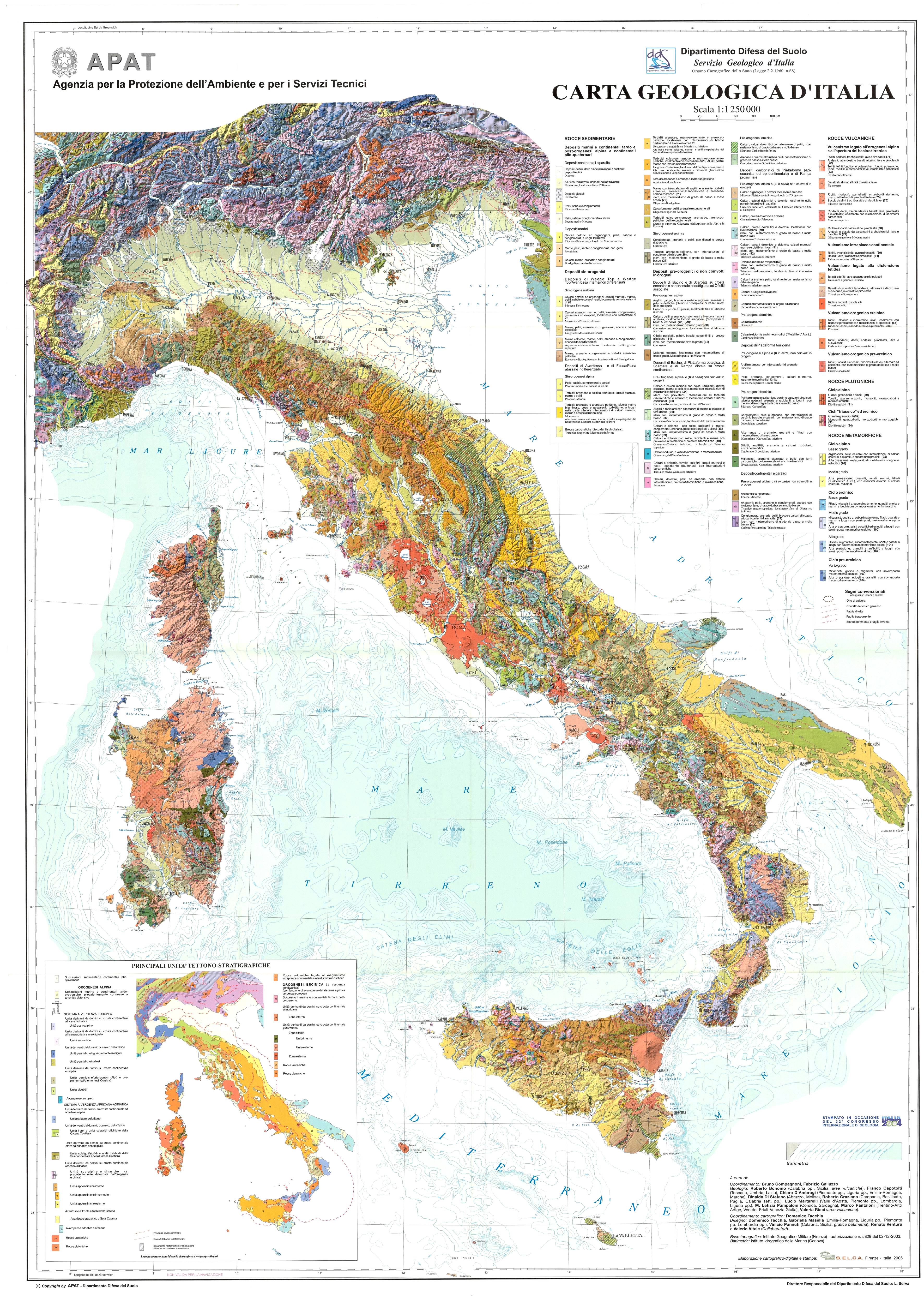
Compagnoni B, Galluzzo F, Bonomo R, Capotorti F, D’Ambrogi C, Di Stefano R, Graziano R, Martarelli L, Pampaloni M L, Pantaloni M, Ricci V, Tacchia D, Masella G, Pannuti V, Ventura R, Vitale V (2004) Carta geologica d’Italia. 32° CGI [Geological map of Italy. 32nd CGI]. https://www.isprambiente.gov.it/images/progetti/progetto-1250-ita.jpg. Accessed July 2023
Dramsch J (2020) 70 years of machine learning in geoscience in review. Adv Geophys 61:1–55. https://doi.org/10.1016/bs.agph.2020.08.002
de Caro M, Perico R, Crosta GB, Frattini P, Volpi G (2020) A regional-scale conceptual and numerical groundwater flow model in fluvio-glacial sediments for the Milan Metropolitan area (northern Italy). J Hydrol Reg Stud 29:100683. https://doi.org/10.1016/j.ejrh.2020.100683
de Graaf IEM, Sutanudjaja EH, van Beek LPH, Bierkens MFP (2015) A high-resolution global-scale groundwater model. Hydrol Earth Syst Sci 19:823–837. https://doi.org/10.5194/hess-19-823-2015
Erofeev A, Orlov D, Ryzhov A, Koroteev D (2019) Prediction of porosity and permeability alteration based on machine learning algorithms. Transp Porous Media 128:677–700. https://doi.org/10.1007/s11242-019-01265-3
Fegh A, Riahi MA, Norouzi GH (2013) Permeability prediction and construction of 3D geological model: application of neural networks and stochastic approaches in an Iranian gas reservoir. Neural Comput Appl 23:1763–1770. https://doi.org/10.1007/s00521-012-1142-8
Gal Y (2016) Uncertainty in deep learning. PhD Thesis, University of Cambridge, Cambridge, UK
Guo J, Li Y, Jessell MW, Giraud J, Li C, Wu L, Li F, Liu S (2021) 3D geological structure inversion from Noddy-generated magnetic data using deep learning methods. Comput Geosci 149:104701. https://doi.org/10.1016/j.cageo.2021.104701
Hallinan JS (2013) Computational intelligence in the design of synthetic microbial genetic systems, chapt 1. In: Methods in microbiology, vol 40. Elsevier, Amsterdam, pp 1–37
Han J, Kamber M, Pei J (2012) Classification. Data Mining. 327-391. https://doi.org/10.1016/B978-0-12-381479-1.00008-3
Harken B, Chang C, Dietrich P, Kalbacher T, Rubin Y (2019) Hydrogeological modeling and water resources management: improving the link between data, prediction, and decision making. Water Resour Res 55:10340–10357. https://doi.org/10.1029/2019WR025227
Hecht-Nielsen R (1989) Neurocomputing : The Technology Of Non-Algorithmic Information Processing
Hillier M, Wellmann F, Brodaric B, de Kemp E, Schetselaar E (2021) Three-dimensional structural geological modeling using graph neural networks. Math Geosci 53:1725–1749. https://doi.org/10.1007/s11004-021-09945-x
Imran M, Alsuhaibani SA (2019) A neuro-fuzzy inference model for diabetic retinopathy classification. In: Intelligent data analysis for biomedical applications. Elsevier, Amsterdam, pp 147–172
ISPRA (2021) Dati geognostici e geofisici [Geognostic and geophysical data]. https://www.isprambiente.gov.it/it/banche-dati/banche-dati-folder/suolo-e-territorio/dati-geognostici-e-geofisici. Accessed October 20, 2022
ISPRA-CARG (2022) Cartografia geologica e geotematica [Geological cartography]. https://www.isprambiente.gov.it/it/progetti/cartella-progetti-in-corso/suolo-e-territorio-1/progetto-carg-cartografia-geologica-e-geotematica. Accessed October 20, 2022
Jia R, Lv Y, Wang G, Carranza E, Chen Y, Wei C, Zhang Z (2021) A stacking methodology of machine learning for 3D geological modeling with geological-geophysical datasets, Laochang Sn camp, Gejiu (China). Comput Geosci 151:104754. https://doi.org/10.1016/j.cageo.2021.104754
Jordan MI, Mitchell TM (2015) Machine learning: trends, perspectives, and prospects. Science (1979) 349:255–260. https://doi.org/10.1126/science.aaa8415
Kamble VH, Dale MP (2022) Machine learning approach for longitudinal face recognition of children. In: Machine learning for biometrics. Elsevier, Amsterdam, pp 1–27
Kempen B, Brus D, Heuvelink G, Stoorvogel J (2009) Updating the 1:50,000 Dutch soil map using legacy soil data: A multinomial logistic regression approach. Geoderma 151(3-4):311–326. https://doi.org/10.1016/j.geoderma.2009.04.023
Kingma DP, Ba J (2014) Adam: a method for stochastic optimization. Open J Stat 11(2)
Kipf TN, Welling M (2016) Semi-supervised classification with graph convolutional networks. ICLR 2017, Toulon, France, April 2017
Maione U, Paoletti A, Grezzi G (1991) Studio di gestione coordinata delle acque di superficie e di falda nel territorio compreso fra i fiumi Adda e Oglio e delimitato dalle Prealpi e dalla linea settentrionale di affioramento dei fontanili [Study on surface and subsurface water management in the area between the Adda and Oglio river, the Prealpi line and the springs line].
Maxwell RM, Condon LE, Kollet SJ (2015) A high-resolution simulation of groundwater and surface water over most of the continental US with the integrated hydrologic model ParFlow v3. Geosci Model Dev 8:923–937. https://doi.org/10.5194/gmd-8-923-2015
Musacchio A, Mas-Pla J, Soana E, Re V, Sacchi E (2021) Governance and groundwater modelling: hints to boost the implementation of the EU Nitrate Directive: the Lombardy Plain case, N Italy. Sci Total Environ 782:146800. https://doi.org/10.1016/j.scitotenv.2021.146800
Patani SE, Porta GM, Caronni V, Ruffo P, Guadagnini A (2021) Stochastic inverse modeling and parametric uncertainty of sediment deposition processes across geologic time scales. Math Geosci 53:1101–1124. https://doi.org/10.1007/s11004-020-09911-z
PdG Po (2015) Piano di gestione del distretto idrografico del fiume Po [Management plan of the hydrographic district of the river Po]. Autorità di Bacino del Fiume Po, Parma, Italy
Pedregosa F, Varoquaux G, Gramfort A, Michel V, Thirion V, Grisel O, Blondal M, Prettenhofer P, Weiss R, Dubourg V, Vanderplas J, Passos A, Cournapeu D, Brucher M, Perrot M, Duchesnay E (2011) Scikit-learn: machine learning in Python. J Mach Learn Res 12(2011):2825–2830
Poggio L, de Sousa LM, Batjes NH et al (2021) SoilGrids 2.0: producing soil information for the globe with quantified spatial uncertainty. SOIL 7:217–240. https://doi.org/10.5194/soil-7-217-2021
Regione Emilia-Romagna (2022) Portale minERva (minERva portal). https://datacatalog.regione.emilia-romagna.it/catalogCTA/dataset?groups=geologia&tags=stratigrafia&publisher_name=Regione+Emilia-Romagna. Accessed October 20, 2022
Regione Lombardia (2022) Banca dati geologica del sottosuolo [Geological data base]. https://www.geoportale.regione.lombardia.it/it/metadati?p_p_id=detailSheetMetadata_WAR_gptmetadataportlet&p_p_lifecycle=0&p_p_state=normal&p_p_mode=view&_detailSheetMetadata_WAR_gptmetadataportlet_uuid=%7BDAF98B21-3257-4D23-9D53-5AECC966D872%7D. Accessed October 20, 2022
Raggi M, Ronchi D, Sardonini L, Viaggi D (2009) Po basin case study status report. AquaMoney, EC, Brussels
Ramadhan RAA, Heatubun YRJ, Tan SF, Lee H-J (2021) Comparison of physical and machine learning models for estimating solar irradiance and photovoltaic power. Renew Energy 178:1006–1019. https://doi.org/10.1016/j.renene.2021.06.079
Sahoo S, Jha MK (2016) Pattern recognition in lithology classification: modeling using neural networks, self-organizing maps and genetic algorithms. Hydrogeol J 25(2):311–330. https://doi.org/10.1007/s10040-016-1478-8
Schroeder W, Martin K, Lorensen B (2006) The visualization toolkit, 4th edn. Kitware. https://vtk.org/download/. Accessed July 2023
Schulz S, Walther M, Michelsen N, Rauch R, Dirks H, Al-Saud M, Merz R, Koldtiz O, Schueth C (2017) Improving large-scale groundwater models by considering fossil gradients. Adv Water Resour 103:32–43. https://doi.org/10.1016/j.advwatres.2017.02.010
Shannon CE (1948) A mathematical theory of communication. Bell Syst Tech J 27:379–423. https://doi.org/10.1002/j.1538-7305.1948.tb01338.x
Singh D, Singh B (2020) Investigating the impact of data normalization on classification performance. Appl Soft Comput 97:105524. https://doi.org/10.1016/j.asoc.2019.105524
Sudakov O, Burnaev E, Koroteev D (2019) Driving digital rock towards machine learning: predicting permeability with gradient boosting and deep neural networks. Comput Geosci 127:91–98. https://doi.org/10.1016/j.cageo.2019.02.002
Tahmasebi P, Kamrava S, Bai T, Sahimi M (2020) Machine learning in geo- and environmental sciences: from small to large scale. Adv Water Resour 142:103619
Tahmasebi P, Sahimi M, Shirangi MG (2018) Rapid learning-based and geologically consistent history matching. Transp Porous Media 122:279–304. https://doi.org/10.1007/s11242-018-1005-6
Takbiri-Borujeni A, Kazemi H, Nasrabadi N (2020) A data-driven surrogate to image-based flow simulations in porous media. Comput Fluids 201:104475. https://doi.org/10.1016/j.compfluid.2020.104475
Titus Z, Heaney C, Jacquemyn C, Salinas P, Jackson MD, Pain C (2021) Conditioning surface-based geological models to well data using artificial neural networks. Comput Geosci. https://doi.org/10.1007/s10596-021-10088-5
Trichakis IC, Nikolos IK, Karatzas GP (2011) Artificial Neural Network (ANN) based modeling for karstic groundwater level simulation. Water Resour Manage 25:1143–1152. https://doi.org/10.1007/s11269-010-9628-6
Varoquaux G (2022) joblib Documentation Release 1.2.0.dev0. https://joblib.readthedocs.io/en/stable/. Accessed July 2023
Venkateswarlu Ch, Karri RR (2022) Data-driven modeling techniques for state estimation. In: Optimal state estimation for process monitoring, fault diagnosis and control. Elsevier, Amsterdam, pp 91–111
Vu MT, Jardani A, Massei N, Fournier M (2021) Reconstruction of missing groundwater level data by using Long Short-Term Memory (LSTM) deep neural network. J Hydrol 597. https://doi.org/10.1016/j.jhydrol.2020.125776
Yang ZR, Yang Z (2014) Artificial Neural Networks. Comprehensive Biomedical Physics. 1–17. https://doi.org/10.1016/B978-0-444-53632-7.01101-1
Zhang G, Wang Z, Li H et al (2018a) Permeability prediction of isolated channel sands using machine learning. J Appl Geophys 159:605–615. https://doi.org/10.1016/j.jappgeo.2018.09.011
Zhang J, Zhu Y, Zhang X, Ye M, Yang J (2018b) Developing a Long Short-Term Memory (LSTM) based model for predicting water table depth in agricultural areas. J Hydrol 561:918–929. https://doi.org/10.1016/j.jhydrol.2018.04.065
Zwingle E (2002) Italy’s Po River punished for centuries by destructive floods, northern Italians stubbornly embrace their nation’s longest river, which nurtures rice fields, vineyards, fisheries and legends. Natl Geogr Mag May 2002
Acknowledgements
The authors are grateful to Paolo Severi from Regione Emilia-Romagna for providing the information about spatial location and lithological data of wells within the Emilia-Romagna region in a unified format. Computations were performed at the High Performance Computing infrastructure CFDHub@Polimi (https://www.cfdhub.polimi.it/).
Funding
Open access funding provided by Politecnico di Milano within the CRUI-CARE Agreement. A. Guadagnini acknowledges funding from the European Union Next-Generation EU (National Recovery and Resilience Plan – NRRP, Mission 4, Component 2, Investment 1.3 – D.D. 1243 2/8/2022, PE0000005) in the context of the RETURN Extended Partnership. M. Riva acknowledges support from Water Alliance – Acque di Lombardia.
Author information
Authors and Affiliations
Corresponding author
Ethics declarations
Conflict of interest
The authors state that there is no conflict of interest.
Additional information
Publisher’s note
Springer Nature remains neutral with regard to jurisdictional claims in published maps and institutional affiliations.
Published in the special issue “Geostatistics and hydrogeology”.
Supplementary Information
Below is the link to the electronic supplementary material.
Rights and permissions
Open Access This article is licensed under a Creative Commons Attribution 4.0 International License, which permits use, sharing, adaptation, distribution and reproduction in any medium or format, as long as you give appropriate credit to the original author(s) and the source, provide a link to the Creative Commons licence, and indicate if changes were made. The images or other third party material in this article are included in the article's Creative Commons licence, unless indicated otherwise in a credit line to the material. If material is not included in the article's Creative Commons licence and your intended use is not permitted by statutory regulation or exceeds the permitted use, you will need to obtain permission directly from the copyright holder. To view a copy of this licence, visit http://creativecommons.org/licenses/by/4.0/.
About this article

Cite this article
Manzoni, A., Porta, G.M., Guadagnini, L. et al. Probabilistic reconstruction via machine-learning of the Po watershed aquifer system (Italy). Hydrogeol J 31, 1547–1563 (2023). https://doi.org/10.1007/s10040-023-02677-8
Received:
Accepted:
Published:
Issue Date:
DOI: https://doi.org/10.1007/s10040-023-02677-8