
Abstract
This paper investigates whether the external consumption habit can be a source of indeterminacy in a one-sector growth model when the labor supply is elastic. When there is a proper habit effect with a positive intertemporal elasticity of substitution, we find that the model exhibits indeterminacy if the coefficient of the habit formation is sufficiently large that allows for a substantial impact of current consumption on the habit. Indeterminacy arises even though the elasticity of the Frisch labor supply is positive and the elasticity of the labor demand in negative. In a calibrated version, we find that indeterminacy is empirically plausible when the habit effect is negative that features the “catching up with the Joneses” effect. Under given “catching up with the Joneses” effects, the external consumption habit can be a source of indeterminacy even if more than a half of the external consumption habit comes from past average consumption.


Notes
The Frisch labor supply is the labor supply when the marginal utility of consumption is constant.
Woodford (1994) found that in a monetary economy with a CIA constraint, the equilibrium path is indeterminate under a given exogenous growth rate of the money supply but is unique under a pegged nominal interest rate.
The concept of the consumption habit may be traced to Hume (1748) who argued that preferences were influenced not simply by what a person did in the past, what his parents did, and what contemporary peers were doing but also by the behavior of past generations of peers. Similar contemporary ideas dated to Marshall (1898), Duesenberry (1949), Leibenstein (1950), and Hicks (1965). Subsequent research has identified two kinds of habit formation. One is referred to as external habit formation, expressed in terms of the past consumption of some outside reference group, usually the past consumption of the overall economy, and is the focus in the current study. The other is termed internal habit formation based upon an individual’s own past consumption level.
Recently, Wirl (2011) has analyzed general conditions for indeterminacy and multiple steady states in a model with an external stock in payoffs wherein the dynamical system includes a control and a stock. There are similarities between Wirl and our paper. First, both papers consider externalities. Moreover, externalities are both generated by stock variables. Finally, both papers derive the conditions that lead to indeterminacy. Our model has a negative externality and is a three-equation dynamical system and is different from a two-equation system in Wirl (2011) which considers a positive externality. Like our paper, the model by Antoci et al. (2009) has negative externalities and is a three-equation dynamical system. Unlike our paper, the negative externalities in the latter paper are generated by aggregate output which generates pollutions and reduces natural resources. Thus, their negative externalities affect the supply side, whereas our negative externalities affect the demand side. Moreover, Antoci et al. (2009) focus on global indeterminacy as opposed to local indeterminacy in our paper.
Evidence of the external habit effect has been prevalent and was confirmed as early as the 1950s by Brown (1952) who estimated the habit effect by using the aggregate data in Canada. Recently, a growing body of empirical evidence concerning external habit persistence has emerged. Using time-series data in the US, Fuhrer (2000) strongly supported the hypothesis of consumption habit formation. More recently, using panel data in the US, Ravina (2005) and Korniotis (2010) both have provided strong evidence about external habit persistence in household consumption choices. Using data from other countries, supportive evidence of external habits has been offered by, among others, van de Stadt et al. (1985) who used longitudinal panel surveys of households in the Netherlands, Guariglia and Rossi (2002) who used the British Household Panel Survey, Case (1991) who used an Indonesian socio-economic survey, and Carrasco et al. (2005) who used household panel data from Spain.
The formulation is different from that in Auray et al. (2002); Auray et al. (2005) which assumed \(H_{t}=C_{t-1}\) and thus their habit is determined by the society’s consumption last period. The Ryder and Heal’s formulation is more general. Constantinides (1990) used the same habit formation regime as ours except his habit is internal.
Readers are referred to the paper by Chen (2007) which found multiple balanced growth paths in a one-sector endogenous growth model with a negative consumption habit effect.
When equilibrium is indeterminate, the equilibrium system cannot pin down the location of initial control variables (consumption) for given initial state variables (capital and habits). Agents’ expectations about other’s behavior affect the location of initial control variables. Since agents’ expectations are like animal’s spirits which can fluctuate a lot, the location of initial control variables fluctuates a lot. Thus, there are endogenous fluctuations in the economy. For a better account, see survey by Benhabib and Farmer (1999).
While \(\sigma +\varsigma >0\), the condition (ii) in Theorem 1 is \(\phi _ +\sigma -\chi <\eta -\varepsilon <0,\) where the sign of \(\eta -\varepsilon <0\) follows from (10a).
Fig. 1 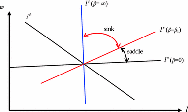
Labor supply and the determinacy of the equilibrium path
The slope of \(\Phi (l,\psi )\) is dictated by \(\textstyle {{d\Phi (l,\psi )} \over {dl}}=\textstyle {1 \over \nu }l^*{\psi (\textstyle {1 \over \nu }-1)-2}\{[\psi (1-v)-v]-\psi (1-v)l\}.\)
While Constantinides (1990) employed \(\beta =0.6\), Carroll et al. (1997) and Alvarez-Cuadrado et al. (2004) used \(\beta =0.2\). Our value lies within these existing values used. As we will see from the quantitative results in Fig. 5 below, there is a tradeoff between the coefficient of the habit formation \(\beta \) and the CUJ effect \(\psi (1-\nu )\). Thus, if we parameterize \(\beta =0.6\), the required CUJ effect that creates indeterminacy is smaller. Alternatively, if we parameterize \(\beta =0.2\), the required CUJ effect that creates indeterminacy is larger.
Prescott (2006) pointed out that 25 % of productive time was allocated to market in the US.
There is another steady state with \(l_{2}^{*}\) \(=\) 0.2674 which is a saddle.

References
Abel AB (1990) Asset prices under habit formation and catching up with the Joneses. Am Econ Rev 80:38–42
Alessie R, Kapteyn A (1991) Habit formation and preference interdependence in the almost ideal demand system. Econ J 101:404–419
Alonso-Carrera J, Caballe J, Raurich X (2006) Welfare implications of the interaction between habits and consumption externalities. Int Econ Rev 47:557–571
Alonso-Carrera J, Caballe J, Raurich X (2008) Can consumption spillovers be a source of equilibrium indeterminacy. J Econ Dyn Control 32:2883–2902
Alvarez-Cuadrado F, Monteiro G, Turnovsky S (2004) Habit formation, catching up with the Joneses, and economic growth. J Econ Growth 9:47–80
Antoci A, Galeotti MG, Russu P (2009) Over-exploitation of open-access natural resources and global indeterminacy in an economic growth model. Mimeo. Universita di Sassari
Auray S, Collard F (2002) Money and external habit persistence: a tale for chaos. Econ Lett 76:121–127
Auray S, Collard F (2005) Habit persistence, money growth rule and real indeterminacy. Rev Econ Dyn 8:48–67
Basu S, Fernald JG (1997) Returns-to-scale in U.S. production: estimates and implications. J Polit Econ 105:249–283
Benhabib J, Farmer REA (1994) Indeterminacy and increasing returns. J Econ Theory 63:19–41
Benhabib J, Farmer REA (1999) Indeterminacy and sunspots in macroeconomics. In: Taylor JB, Woodford M (eds) Handbook of macroeconomics, vol 1. Elsevier, Amsterdam, pp 388–448
Bennett RL, Farmer RE (2000) Indeterminacy with non-separable utility. J Econ Theory 93:118–143
Brown TM (1952) Habit persistence and lags in consumer behavior. Econometrica 20:355–371
Campbell J, Cochrane J (1999) By force of habit: a consumption-based explanation of aggregate stock market behavior. J Polit Econ 107:205–251
Carrasco R, Labeaga JM, Lopez-Aslido JD (2005) Consumption and habits: evidence from panel data. Econ J 115:144–165
Carroll CD, Overland J, Weil DN (1997) Comparison utility in a growth model. J Econ Growth 2:339–367
Carroll CD, Overland J, Weil DN (2000) Saving and growth with habit Formation. Am Econ Rev 90:341–355
Case A (1991) Spatial patterns in household demand. Econometrica 59:953–965
Chen BL (2007) Multiple BGPs in a growth model with habit persistence. J Money Credit Bank 39:25–48
Chen BL, Hsu M (2007) Admiration is a source of indeterminacy. Econ Lett 95:96–103
Chen BL, Hsu M, Hsu YS (2010) A one-sector growth model with consumption standard: indeterminate or determinate. Jpn Econ Rev 61:85–96
Constantinides GM (1990) Habit formation: a resolution of the equity premium puzzle. J Polit Econ 98(3):519–543
Cooper R, John A (1988) Coordinating coordination failures in Keynesian models. Q J Econ 103:441–463
Doi J, Mino K (2008) A variety-expansion model of growth with external habit formation. J Econ Dyn Control 32:3055–3083
Drugeon JP (1998) A model with endogenously determined cycles, discounting and growth. Econ Theory 12:349–369
Duesenberry JS (1949) Income, saving, and the theory of consumer behavior. Oxford University Press, New York
Farmer R, Guo J-T (1994) Real business cycles and the animal spirits hypothesis. J Econ Theory 63:42–72
Fuhrer J (2000) Habit formation in consumption and its implications for monetary-policy models. Am Econ Rev 90:367–390
Guariglia A, Rossi M (2002) Consumption, habit formation, and precautionary saving: evidence from the British Household Panel Survey. Oxf Econ Pap 54:1–19
Hicks JR (1965) Capital and growth. Clarendon Press, Oxford
Hintermaier T (2003) On the minimum degree of returns to scale in sunspot Models of the business-cycle. J Econ Theory 110:400–409
Hume D (1748) An enquiry concerning human understanding, reprinted, 1955. The Bobbs-Merrill Company Inc., Indianapolis
Korniotis GM (2010) Estimating panel models with internal and external habit formation. J Bus Econ Stat 28:145–158
Leibenstein H (1950) Bandwagon, snob, and Veblen effects in the theory of consumers’ demand. Q J Econ 64:183–207
Liu WF, Turnovsky S (2005) Consumption externalities, production externalities, and long-run macroeconomic efficiency. J Public Econ 89:1097–1129
Marshall AA (1898) Principles of economics, 8th edn. Macmillan, New York
Prescott EC (2006) Nobel lecture: the transformation of macroeconomic policy and research. J Polit Econ 114:203–235
Ravina E (2005) Habit persistence and keeping up with the Joneses: evidence from micro data. Working Paper, New York University
Ryder HE, Heal GM (1973) Optimum growth with intertemporally dependent preferences. Rev Econ Stud 40:1–33
van de Stadt H, Kapteyn A, van de Geer S (1985) The relativity of utility: evidence from panel data. Rev Econ Stat 67:179–187
Veblen T (1899) The theory of the leisure class: an economic study of institutions. George Allen and Unwin, London
Wirl F (2011) Conditions for indeterminacy and thresholds in neoclassical growth models. J Econ 102:193–215
Woodford M (1994) Monetary policy and price level determinacy in a cash-in-advance economy. Econ Theory 4:345–380
Acknowledgments
We thank two anonymous referees for valuable comments. We benefited from suggestions made by Jang-Ting Guo, Chong K. Yip and participants at the 2010 Meeting of the Society of Advanced Economic Theory (SAET) held in Singapore.
Author information
Authors and Affiliations
Corresponding author
Appendices
Appendix 1: The elasticity of the Frisch labor supply
If we differentiate (5a) and keep \(\lambda \) fixed, we obtain
Under given \(\lambda \), differentiating (5b) gives
Substituting (19) into (20) yields
and thus the elasticity of the Frisch labor supply
In order to obtain dH/dC, we rewrite \(H_{t}\) as
where \(D(t,\tau )=\beta e^{-\beta (\tau -t)}\) which satisfies
Hence, \(D(t,\tau )\) measures the influence of \(C_{\tau }\) on \(H_{t}\) at time \(\tau \in (-\infty ; t]\) and is thus a weight function defined on \(\tau \in (-\infty ; t]\) with the total weight equal 1 for all \(\beta >0\). \(D(t,\tau )\) is a decreasing function of \(\beta \) for \(\beta \ge \textstyle {1 \over {t-\tau }}\) that approaches 0 as \(\beta \rightarrow \infty \). Thus, as \(\beta \rightarrow \infty \), \(D(t, \tau )\) approaches to the function \(\Upsilon _{t }(\tau )\) that satisfies
and \(\int _{-\infty }^t {\Upsilon _t (\tau )d\tau =1.} \) This indicates that for \(\beta \rightarrow \infty \), \(H_{t}=C_{t}\).
To explore further how the change in \(C_{t}\) affects \(H_{t}\), let us consider the case wherein \(C_{\tau }\) is changed to \(C_{\tau }+dC_{\tau }\) and \(H_{t}\) is changed to \(H_{t}+dH_{t}\). Using (22), we obtain
We assume that for some \(t_{1}<t\),
Denote \(\Delta t=t-t_{1}>0\). Then by (24), \(dH_t =(1-e^{-\beta \Delta t})q\) and the effect of the change in \(C_{t}\) on \(H_{t}\) becomes \(x(\beta )\equiv \textstyle {{dH_t } \over {dC_\tau }}=\textstyle {{dH_t } \over q}=(1-e^{-\beta \Delta t}).\) One can see that \(0<x(\beta )<1\) and \(x(\beta )\) is increasing in \(\beta \), with \(x(\beta )\rightarrow 0\) as \(\beta \rightarrow 0\) and \(x (\beta )\rightarrow 1\) as \(\beta \rightarrow \infty \).
Therefore, (21) can be rewritten as
Appendix 2: Proof of Theorem 1
In the Appendix, we prove the Theorem 1. Denote \(f_{i}\), \(i=l\), \(k\) and \(lj\), \(j=C\), \(k\), \(H\), as partial derivatives with respect to \(i\) and \(j\). If we take the linear Taylor’s expansion of the dynamic equilibrium system (2), (6c) and (16) in the neighborhood of a steady state, along with the use of (8), we obtain
where
Let \(J\) denote the Jacobean matrix in (25) and \(\omega \) denote its corresponding eigenvalue. The characteristic polynomial is in (11), with Det(\(J)\), Tr(\(J)\) and Ds(\(J)\) defined in (12a)–(12c).
It is clear from (11) that \(G(\omega )=-\infty \) when \(\omega =\infty \) and \(G(\omega )=\infty \) when \(\omega =-\infty \). A sink requires three stable roots. The necessary conditions for the presence of three stable roots are: (i) \(G(0)=Det(J)<0\) and (ii) \(G^{\prime }(0)=-Ds(J)<0\). Moreover, according to the Routh-Hurwitz theorem, the requirement of no eigenvalues with positive real parts in the above characteristic polynomial suggests no variation in signs in the following series: \(\left\{ {-1, Tr( J),_ -Ds( J)+Det( J)/Tr( J), Det( J)} \right\} .\) This indicates the additional requirement of (iii) Tr \((J)<0\) and (iv) \(-Ds( J)+Det( J)/Tr( J)<0.\)
To investigate these conditions,
-
(i)
\(G( 0)=Det( J)<0\) Since \(Det( J)=\beta ( {1-\alpha })( {\rho +\delta })\left[ {\rho +\delta ( {1-\alpha })} \right][(\phi +\sigma +\varepsilon -\eta )-\chi ]\)/(-\(\Omega \alpha )\) and \(\Omega <0\), it is obvious that this requires \(\chi >\phi +\sigma -\eta +\varepsilon \).
-
(ii)
\(Tr( J)<0\). As \(T>0\), Tr \((J)<0\) requires both
$$\begin{aligned} \Gamma _{1}<0 \quad \text{ and}\quad \beta >\beta _{a}\equiv T/(-\Gamma _{1})>0. \end{aligned}$$(26a) -
(iii)
\(G^{\prime }(0)= -Ds(J)<0\) As \(M<0, Ds(J)\,>\,0\) requires both
$$\begin{aligned} \Gamma _2 >0 \quad \text{ and}\quad \beta >\beta _b \equiv M/( {-\Gamma _2 })>0. \end{aligned}$$(26b) -
(iv)
\(-Ds(J)+Det(J)/Tr(J)<0\) Under Tr \((J)<0\) in (ii), condition (iv) is equivalent to \(-Ds(J)Tr(J)+Det(J)>0\). Using (12a)–(12c), this requires
$$\begin{aligned} L(\beta )=\beta ^2-\beta \left\{ \frac{M}{-\Gamma _2}+\frac{T}{-\Gamma _1}+ \frac{N}{-\Gamma _1 \Gamma _2}\right\} + \frac{MT}{\Gamma _1 \Gamma _2}>0, \end{aligned}$$(27a)where \(N=\textstyle {{(1-\alpha )(\rho +\delta )} \over {(-\Omega )}}\textstyle {{\rho +\delta (1-\alpha )} \over \alpha }(\phi +\sigma -\eta +\varepsilon -\chi )<0,\) whose the negative sign comes from using (i).
When \(L({\beta })=0\) the polynomial has two roots \({\beta }_{1}\) and \({\beta }_{2 }, {\beta }_{1}\ge {\beta }_{2}\), as follows.
Under (i) Det \((J)<0\), (ii) Tr \((J)<0\) and (iii) Ds \((J)>0\), both \({\beta }_{1}\) and \({\beta }_{2}\) are positive, as verified by
The inequality sign in (26a) is satisfied if any one of the following two cases holds: (a) \(\beta >\beta _{1}\ge \beta _{2}\) or (b) \(\beta <\beta _{2}\le \beta _{1}\). However, case (b) is impossible as case (b) implies \(\beta _{2}<T/(-\Gamma _{1})\equiv \beta _{a}\), which is against the requirement of \(\beta >\beta _{a}\) for Tr \((J)<0\) in (ii).
Therefore, (27a) and \(-Ds(J)Tr(J)+Det(J)>0\) both can be met only if
It is straightforward to show that \(\beta _{1}>\beta _{a}\) and \(\beta _{1}>\beta _{b}\). Thus, (26a), (26b) and (27b) indicate that the requirement of \(\beta >\beta _{1}\).
Therefore, under \(\beta >\beta _{1}\), the conditions of a sink are: \(\chi >\phi +\sigma -\eta +\varepsilon \), \(\Gamma _{1}<0\) and \(\Gamma _{2}>0\).
Rights and permissions
About this article
Cite this article
Chen, BL., Hsu, YS. & Mino, K. Can consumption habit spillovers be a source of equilibrium indeterminacy?. J Econ 109, 245–269 (2013). https://doi.org/10.1007/s00712-012-0301-9
Received:
Accepted:
Published:
Issue Date:
DOI: https://doi.org/10.1007/s00712-012-0301-9