
Abstract
We show that the N(1440) Roper resonance naturally appears in the nuclear model with explicit mesons as a structure in the continuum spectrum of the physical proton, which in this calculation is made of a bare nucleon dressed with a pion cloud.
1 Introduction
The N(1440) Roper resonance is a relatively broad nucleon resonance with the mass of about 1440 MeV and the width of about 350 MeV [1]. While the exact nature of the resonance is still debated (see [2,3,4,5] and references therein), one line of thought is that it consists of a quark core augmented by a meson cloud. This concurs well with the nuclear model with explicit mesons (MEM) where the physical nucleon is made of a bare nucleon—the quark core—dressed with a meson cloud [6, 7]. One might therefore expect that in MEM the Roper resonance should somehow reveal itself in the continuum spectrum of the physical proton.
In this contribution we investigate the continuum spectrum of the physical proton within one-pion MEM in the hope to identify the Roper resonance and establish the parameters of MEM that are consistent with the tabulated mass and width of the resonance. The method we use is calculation of the strength-function of a certain fictional reaction, where the proton is excited from the ground state into continuum, with the subsequent fit of the calculated strength-function with a Breit-Wigner distribution.
2 The Physical Nucleon in MEM
The MEM is a nuclear interaction model, based on the Schrödinger equation, where the nucleons do not interact with each other via a potential but rather emit and absorb mesons [6, 7]. The mesons are treated explicitly on the same footing as the nucleons.
The physical nucleon in MEM is represented by a superposition of states where the bare nucleon is surrounded by different number of (virtual) mesons. In one-pion approximation the physical nucleon is a superposition of two states: the bare nucleon, and the bare nucleon surrounded by one pion. The corresponding wave-function of the physical nucleon, \(\Psi \), is a two-component vector,
where \(\psi _0\) is the (wave-function of the) state with the bare nucleon and no pions, \(\psi _1\)—the state with a bare nucleon and one pion, \(\vec R\) is the coordinate of the center-of-mass of the system, and \(\vec r\) is the coordinate between the bare nucleon and the pion.
The Hamiltonian H that acts on this wave-function is a matrix,
where \(K_N, K_\pi \) are kinetic energy operators for the bare nucleon and the pion, \(m_N\) and \(m_\pi \) are masses of the bare nucleon and the pion, and W and \(W^\dagger \) are pion emission and absorption operators (also called the nucleon-pion coupling operators).
The corresponding Schrödinger equation is given as
with the normalization condition
where E is the energy of the system and V is the normalization volume.
The simplest W-operator that is consistent with conservation of isospin, angular momentum, and parity can be written as
where \(\vec \sigma \) is the vector of Pauli matrices that act on the spin of the nucleon, \(\vec \tau \) is the isovector of Pauli matrices that act on the isospin of the nucleon,Footnote 1 and where F(r) is a (short-range) form-factor. The dimension of W is \(E/\sqrt{V}\), therefore it might be of convenience to choose
where f(r) is normalized such that
in which case the strength factor \(S_w\) has the dimension of energy and one can (hopefully) meaningfully compare form-factors of different shapes.Footnote 2
3 The Semi-Relativistic Schrödinger Equation
3.1 The Two-Component Wave-Function
The \(\psi _0\)-component of the two-component wave-function \(\Psi \) in (1) represents a single bare proton at rest in the volume V. This component can be chosen as
where p is the proton isospin state,
and where \(\uparrow \) is the spin-up state,
and where \(c_0\) is a dimensionless normalization constant.
With this \(\psi _0\) the inhomogeneous term, \(W\psi _0\), in the second row of the Schrödinger equation (3) takes the the form
Since all terms in that equation should have the same spin-isospin structure one has to conclude that the component \(\psi _1\) is bound have the same form as \(W\psi _0\), that is,
where \(\phi (r)\) is a (yet unknown) scalar function.
Therefore we are going to search for the wave-function of the physical proton (in the center-of-mass system) in the form
where the constant \(c_0\) and the function \(\phi (r)\) are to be found by solving the corresponding Schrödinger equation.
The normalization condition the function \(\Psi \) is given asFootnote 3
3.2 The Schrödinger Equation
With the ansatz (16) the Schrödinger equation (3) turns into the following system of equations for the constant \(c_0\) and the function \(\phi (r)\),
It is of advantage to introduce the radial function u(r),
with the simple boundary condition at the origin,
and the normalization condition
For the u(r) function the Schrödinger equation becomes
In the center-of-mass frame the nucleon and the pion have equal momenta with opposite signs, \(-\vec p\) and \(\vec p\). Their (relativistic) kinetic energies are therefore given as
The momentum as a quantum-mechanical operator in coordinate space is given as
Correspondingly the kinetic energies operators are
With these kinetic energies the Schrödinger equation turns into the following system of integro-differential equations,
where the function
is representable by a Maclaurin series.Footnote 4
The single action of the \(\nabla ^2\) operator on \(\frac{\vec r}{r^2}u(r)\) is given as
where the action of the operator \({\hat{D}}\) is defined as
Repeating the action suggests that for any non-negative integer n
Therefore for any function f(x) that can be represented as a power series the following holds true,
Inserting this into (27) gives, finally, the sought semi-relativistic radial Schrödinger equation for the physical proton in one-pion MEM,
with the boundary condition \(u(0)=0\).
4 Numerical Solution of the Schrödinger Equation
The system of Eqs. (34) can be solved numerically by discretizing the r-variable and using finite-difference approximations for the derivatives and integrals.
Let us introduce a regular grid,
where \(\Delta r\) is the grid spacing. The integral in the first equation in (34) can then be approximated as
Introducing the auxiliary tilde-variables,
the system of Eqs. (34) turns into the following form,
where the numbers \(f_K({\hat{D}})_{ij}\) are the matrix elements of the matrix representation of the operator \(f_K({\hat{D}})\) on the grid; and where applies the ordinary matrix normalization condition,
The system of Eqs. (38) with the normalization condition (39) is in fact a real symmetric matrix eigenproblem,
where the Hamiltonian matrix \({\mathcal {H}}\) is given as
The \({\hat{D}}\) operator on the grid can be built using the second order central finite-difference approximation for the second derivative,
which gives
Now the matrix \(f_K({\hat{D}})\) can be built in the following way: if \(\lambda _i\) and \(v_i\) are the eigenvalues and eigenvectors of the \({\hat{D}}\) operator,
then the matrix representation of any Maclaurin expandable operator \(f({\hat{D}})\) is given as
where V is the matrix of eigenvectors \(v_i\) and where \(f(\lambda )\) is a diagonal matrix with diagonal elements \(f(\lambda _i)\).
The Hamiltonian matrix built this way has the bounding box boundary conditions inbuilt,
where \(R_\textrm{max}=(n+1)\Delta r\). Diagonalization of this Hamiltonian matrix produces one state, \({\tilde{u}}^{(0)}(r)\), with the energy below \(m_N\) (this state is the physical protonFootnote 5—the bound state of the bare proton and the pion) and n discretized-continuum states, \({\tilde{u}}^{(k=1\dots n)}(r)\), with energies above the pion emission threshold.Footnote 6 These states decay into a nucleon and a pion, and the Roper resonance, if any, must be lurking somewhere there.
Mathematically the exact continuum spectrum is recovered in the limit \(R_\textrm{max}\rightarrow \infty \), \(\Delta r\rightarrow 0\). However in practice the discretized calculations converge when \(R_\textrm{max}\) is much larger than, and \(\Delta r\) is much smaller than, the typical length of the system given by the interaction range \(b_w\sim 1.5\)fm. As illustrated in the Appendix the discretized calculations converge to within about three decimal digits when \(R_\textrm{max}/b_w\sim b_w/\Delta r\sim 20\).
An example of the radial eigenfunctions \({\tilde{u}}^{(k)}(r)\) is shown on Fig. 1: the ground state is a localised bound state of the bare nucleon and the pion; the “below-resonance” continuum wave-function shows little presence at the shorter distances; the “on-resonance” wave-function has a much larger amplitude in the inner region.

The radial wave-functions \({\tilde{u}}^{(k)}(r)\): the ground (bound) state wave-function \({\tilde{u}}^{(0)}\), a below-resonance continuum wave-function \({\tilde{u}}^{(3)}\), and an on-resonance continuum wave-function \({\tilde{u}}^{(20)}\). The model parameters are the ones in the first line in Table 1, the discretization parameters are \(\Delta r\)=0.08 fm, \(R_\textrm{max}=35\)fm
5 The Strength-Function of a Fictional Reaction
A resonance is usually identified as a peak in a reaction cross-section with an approximately Breit-Wigner shape. The Roper resonance decays largely (55–75% [1]) into a nucleon and a pion, therefore it should be possible to observe this resonance in a reaction where our dressed proton is excited from the ground state into a continuum spectrum state (which decays into a nucleon and a pion).
Let us consider a reaction where a proton undergoes a transition, caused by a certain operator \({\hat{X}}\), from the ground state \(\Psi _0\) to a state in the continuum \(\Psi _i\) (which then decays into a nucleon and a pion). The amplitude of this quantum transition is given, in the Born approximation, by the matrix element
Since a resonance should not depend on the way the state \(\Psi _i\) is populated, the particular form of the \({\hat{X}}\) operator should be unimportant (as long as the matrix element is not identically zero) and one can just as well use a fictional operator. We have chosen the following matrix element,
as experimentation shows that this one produces the best looking strength-functions (see below).
The cross-section of an excitation reaction into continuum states with energies \(E\pm \frac{\Delta E}{2}\) is determined by the so called strength-function, S(E), which is defined as
In the box-discretized approximation, that we use here, the strength-function of a transition into a discretized-continuum state i with the energy \(E_i\) is given as
where \(\Delta E_i=E_{i+1}-E_i\).
One can determine the parameters of a resonance, the mass and the width, by applying a Breit-Wigner fit to the strength-function S(E) [8]. Unfortunately the Roper resonance is broad and is located close to threshold making it necessary to use a width that is energy-dependent. We shall use the following phenomenological parametrization of the strength-function (cf. [9]),
where
\(\theta \) is the step function, \(E_\textrm{th}\) is the threshold energy, and where the mass M, width \(\Gamma \), and power p are the fitting parameters (\(p\sim 1\)).
6 Results
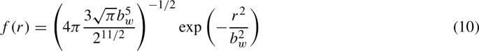
We use the Gaussian form-factor in the normalized form (10),
where the strength, \(S_w\), and the range, \(b_w\), are the model parameters that are varied to reproduce the given mass M and width \(\Gamma \) of the resonance.
Exploratory calculations show that it is possible to reproduce the tabulated mass of the Roper resonance, 1440 Mev, and any given width within the tabulated limits, 250–450 MeV, within a relatively narrow range of the model parameters as indicated in Table 1 and on Fig. 2.

7 Conclusion
We have shown that in the nuclear model with explicit mesons (MEM) the Roper resonance appears as a structure in the continuum spectrum of the physical proton (in one-pion MEM the physical proton is made of a bare nucleon dressed with a pion). We have established the range of the model parameters (the strength and the range of the nucleon-pion coupling operator) that reproduce the tabulated mass and width of the resonance. With these parameters the pion component in the physical proton takes about 10% of the norm of the wave-function and reduces the mass of the bare proton by about 5%. These numbers are much smaller then the corresponding estimates from the pion photo-production cross-section calculation [7]. One source of the discrepancy could be the plane-wave approximation of the continuum states in [7], whereby all effects of interactions in the final state (including the Roper resonance) were disregarded. It seems that these effects are not negligible and must always be taken into account.
Data Availability
No datasets were generated or analysed during the current study.
Notes
The isospin factor \(\vec \tau \vec \pi \) is given as

where \(\pi ^0\), \(\pi ^+\), and \(\pi ^-\) are the physical pions and where the \(\tau \)-matrices are given as

The Gaussian form-factor normalized according to (9) is given as
taking into account the following equations,


To be absolutely correct, the mass \(m_N\) of the bare nucleon must be larger than the nucleon’s physical mass such that adding the pion binding energy produces the observed physical mass of the dressed nucleon. However in all our examples later on the binding energy of the pion is of about 3 to 8% of the nucleon mass and therefore in this exploratory investigation we neglect this effect and assume that \(m_N\) equals the physical mass of the nucleon.
The pion threshold in these calculations corresponds to a decay into a bare nucleon and a pion, meaning that in the threshold energy, \(E_\textrm{th}=m_N+m_\pi \), \(m_N\) is strictly speaking the mass of the bare nucleon that is larger than the physical mass by the binding energy of the virtual pion. In reality the emitted bare nucleon immediately gets dressed with another virtual pion which reduces its mass back to the physical mass, restoring the correct threshold. However this mechanism is not included in the current one-pion approximation. However since the binding of the virtual pion in the present calculations is always small we assume that \(m_N\) is the physical mass.


References
R.L. Workman, Particle Data Group et al., Prog. Theor. Exp. Phys. 2022, 083C01 (2022)
D. B. Leinweber at. al, "Understanding the nature of baryon resonances", to appear in the proceedings of HADRON (2023) arXiv:1710.02549
V.D. Burkert, C.D. Roberts, Roper resonance: toward a solution to the fifty year puzzle. Rev. Mod. Phys. 91, 011003 (2024)
J. Rodriguez-Quintero et al., Form factors for the Nucleon-to-Roper electromagnetic transition at large-Q2. EPJ Web Conf. 241, 02009 (2020)
B. Golli, H. Osmanovic, S. Sirca, A. Svarc, Genuine quark state versus dynamically generated structure for the Roper resonance. Phys. Rev. C 97, 035204 (2018). arXiv:1709.09025
D.V. Fedorov, A nuclear model with explicit mesons. Few-Body Syst. 61, 40 (2020). arXiv:2006.05851
D.V. Fedorov, M. Mikkelsen, Threshold photoproduction of neutral pions off protons in nuclear model with explicit mesons. Few-Body Syst. 64, 3 (2023). arXiv:2209.12071
D.V. Fedorov, A.S. Jensen, M. Thøgersen, Calculating few-body resonances using an oscillator trap. Few-Body Syst. 45, 191 (2009). arXiv:0902.1110
F. Giacosa, A. Okopinska, V. Shastry, A simple alternative to the relativistic Breit-Wigner distribution. Eur. Phys. J. A 57, 336 (2021). arXiv:2106.03749
Funding
Open access funding provided by Aarhus Universitet
Author information
Authors and Affiliations
Contributions
D.V.F. wrote the manuscript and prepared the figures.
Corresponding author
Ethics declarations
Conflict of interest
The authors declare no competing interests.
Additional information
Publisher's Note
Springer Nature remains neutral with regard to jurisdictional claims in published maps and institutional affiliations.
Appendix: Numerical Convergence
Appendix: Numerical Convergence
Figures 3 and 4 illustrate the convergence of the strength-function with respect to variation of the bounding box parameter \(R_\textrm{max}\) and the discretization parameter \(\Delta r\). The figures seem to indicate that the strength-function converges within the width of the line on the figure when \(R_\textrm{max}=30\)fm and \(\Delta r=0.08\)fm. Relative to the characteristic scale of the system—the interaction range parameter \(b_w\sim 1.5\)fm—that gives \(R_\textrm{max}/b_w\sim 20\) and \(b_w/\Delta r\sim 20\).

Convergence of the strength-function \(S(E_i)\) with respect to the bounding box parameter \(R_\textrm{max}\). The interaction parameters \(S_w\) and \(b_w\) are taken from the first row of Table 1, the discretization parameter \(\Delta r=0.08\)fm. The lines are for guiding the eye

Convergence of the strength-function \(S(E_i)\) with respect to the discretization parameter \(\Delta r\). The interaction parameters \(S_w\) and \(b_w\) are taken from the first row of Table 1, the bounding box parameter \(R_\textrm{max}=30\)fm. The lines are for guiding the eye
Rights and permissions
Open Access This article is licensed under a Creative Commons Attribution 4.0 International License, which permits use, sharing, adaptation, distribution and reproduction in any medium or format, as long as you give appropriate credit to the original author(s) and the source, provide a link to the Creative Commons licence, and indicate if changes were made. The images or other third party material in this article are included in the article’s Creative Commons licence, unless indicated otherwise in a credit line to the material. If material is not included in the article’s Creative Commons licence and your intended use is not permitted by statutory regulation or exceeds the permitted use, you will need to obtain permission directly from the copyright holder. To view a copy of this licence, visit http://creativecommons.org/licenses/by/4.0/.
About this article

Cite this article
Fedorov, D.V. The N(1440) Roper Resonance in the Nuclear Model with Explicit Mesons. Few-Body Syst 65, 32 (2024). https://doi.org/10.1007/s00601-024-01899-0
Received:
Accepted:
Published:
DOI: https://doi.org/10.1007/s00601-024-01899-0