
Abstract
We show that there are continuous, \(W^{1,p}\) (\(p<d-1\)), incompressible vector fields for which uniqueness of solutions to the continuity equation fails.
1 Introduction
In this paper we consider the continuity equation
in a d-dimensional periodic domain, \(d \ge 3\), for a time-dependent incompressible vector field \(u : [0,1] \times {\mathbb {T}}^d \rightarrow {\mathbb {R}}^d\) and an unknown density \(\rho : [0,1] \times {\mathbb {T}}^d \rightarrow {\mathbb {R}}\). Here and in the sequel \({\mathbb {T}}^d = {\mathbb {R}}^d/{\mathbb {Z}}^d\) is the d-dimensional flat torus. We will also always assume, without loss of generality, that the time interval is [0, 1]. We prove in these notes the following theorem.
Theorem 1.1
(Non-uniqueness for Sobolev and continuous vector fields). Let \(\varepsilon >0\), \({{\bar{\rho }}} \in C^\infty ({\mathbb {T}}^d)\) with \(\int _{{\mathbb {T}}^d}{{\bar{\rho }}}\,dx=0\). Then there exist
such that \((\rho ,u)\) is a weak solution to (1) and \(\rho (0) \equiv 0\) at \(t=0\), \(\rho (1) \equiv {{\bar{\rho }}}\) at \(t=1\) and
By weak solution we mean solution in the sense of distributions.
We have chosen the periodic setting for simplicity and to emphasize that the key phenomenon we are studying is the effect of (local) low regularity. As with other applications of convex integration (e.g. [9, 14]), we expect that analogous statements hold also in the full space \({\mathbb {R}}^d\).
It is well known that the theory of classical solutions to (1) is closely connected to the ordinary differential equation
via the formula \(\rho (t) {\mathcal {L}}^d = X(t)_\sharp (\rho (0){\mathcal {L}}^d)\) or, equivalently, due to the incompressibility,
In particular, for Lipschitz vector fields u the well-posedness theory for (1) follows from the Cauchy–Lipschitz theory for ordinary differential equations applied to (3).
It is in general of great interest to investigate the existence and uniqueness of weak solutions to the Cauchy problem for (1) in the case of non-smooth vector fields, and the connection to the Lagrangian problem (3), (4). The general question can be formulated as follows. Fix an exponent \(r \in [1,\infty ]\), denote by \(r'\) its dual Hölder, \(1/r + 1/r' = 1\), and assume that a vector field
is given. What can be said about existence and uniqueness of weak solutions in the class of densities
The choice of class (6) for \(\rho \) is motivated by the fact that for classical solutions to (1) every spatial \(L^{r'}\) norm is preserved in time. Once (6) is fixed, the choice of the class (5) for u is natural, since in this way \(\rho u \in L^1((0,1) \times {\mathbb {T}}^d)\) and thus the notion of distributional solution to (1) is well defined.
While existence of weak solutions can be easily shown under the assumptions (5), (6), the uniqueness question is much harder. In 1989 DiPerna and Lions [11] proved that uniqueness holds in the class (6) if
i.e. if u enjoys Sobolev regularity with exponent r. Moreover, in this case, the incompressibility assumption can be relaxed to \(\text {div }u \in L^\infty \). In the class of bounded densities the uniqueness result was later extended by Ambrosio [1] in 2004, for fields \(u \in L^1(0,1; BV)\) with \(\text {div }u \in L^\infty \) and very recently by Bianchini and Bonicatto [3] in 2017 in the case of BV nearly incompressible vector fields.
In all of these results an important additional feature is the connection to a suitable extension to (3), i.e. the link between the Eulerian and the Lagrangian picture. More precisely, under assumption (7), there exists a unique distributional solution to (3) for a.e. x, such that \(x \mapsto X(t,x)\) is measure preserving for all t (assuming \(\text {div }u = 0\)): such flow map is called regular Lagrangian flow (see [2] for a general discussion). Then the unique solution to the continuity or the transport equation is given by (4), as in the smooth case.
On the other side, several non-uniqueness counterexamples are known, but they mainly concern the case when the field is “very far” from being incompressible (e.g. \(\text {div }u \notin L^\infty \), see [11]) or the case when no bounds on one full derivative of u are available (see, for instance, the counterexample in [11] for a field \(u \in L^1 (0,1; W^{s,1})\) for every \(s<1\), but \(u \notin L^1(0,1; W^{1,1})\) or the counterexample in [10] for a field \(u \in L^1(\varepsilon , 1; BV)\) for every \(\varepsilon >0\), but \(u \notin L^1(0,1; BV)\)). In all these counterexamples, however, non-uniqueness for the PDE (1) is a consequence of a Lagrangian non-uniqueness for the associated ODE (3). We refer to [16] and to [2] for a more detailed discussion.
Very recently, we proved in [16] the analog of Theorem 1.1, for fields and densities in the class
with
and
The result in [16] shows that uniqueness can fail even for incompressible, Sobolev vector fields (i.e. fields for which the Lagrangian problem (3) is well posed, in the sense of the regular Lagrangian flow), if the integrability exponent p of Du is much lower than the one provided in (7) by DiPerna and Lions’ theory, as specified in (9).
The end-point \(r=\infty \), corresponding in (9) to \(p < d-1\), is excluded in [16]. The main result of this notes, namely Theorem 1.1, shows that such end-point case can indeed be reached and, in addition, quite surprisingly, the vector field produced by Theorem 1.1 is continuous in time and space, not only bounded.
We postpone to Sect. 2 a technical discussion about why the case \(r=\infty \) was out of reach in [16] and which new ideas are introduced in these notes to deal with such problem.
We would like now to briefly comment about the continuity of the vector field u produced by Theorem 1.1. It was observed by Caravenna and Crippa [7] that the boundedness or the continuity of the vector field (in addition to some Sobolev regularity) could play a key role in the uniqueness problem in the class of integrable densities \(\rho \in L^1((0,1) \times {\mathbb {T}}^d)\). It thus turns out to be a very interesting question to ask if, in fact, boundedness or continuity plus Sobolev regularity are enough to guarantee uniqueness. Theorem 1.1 shows that this is not the case, if the integrability of Du is lower than a dimensional threshold (precisely, \(d-1\)).Footnote 1
The idea that the boundedness or the continuity of u can play a crucial role in the uniqueness problem is confirmed by the fact that the majority of the result concerning existence and uniqueness of the regular Lagrangian flow associated to a Sobolev or BV vector field u assume that \(u \in L^\infty \) (see, for instance, the recent survey [2]).
On a different point of view, it is a classical result (see, for instance, [12]) that the boundedness of u, even without any further Sobolev regularity, is enough to have uniqueness, if a small viscosity is added to the continuity equation:
while in [16] we showed that uniqueness for (10) can drastically fail is u is Sobolev, but not bounded.
The result in Theorem 1.1 is quite surprising, even in comparison with our previous result in [16]. Indeed, for vector fields produced by Theorem 1.1 the Lagrangian picture is very well behaved: first, the Sobolev regularity implies the existence and uniqueness of the regular Lagrangian flow. Second, the continuity of the field implies that the trajectories provided by the regular Lagrangian flow are \(C^1\) in time (and this was not the case for the fields produced in [16]). Third, the bound (2) means that the length of each trajectory is at most \(\varepsilon >0\), i.e. particles almost don’t move (and, again, this was not the case for the fields produced in [16]). Observe also that \(\varepsilon \) in (2) depends neither on the length of the time interval [0, 1] nor on the \(L^1\) distance between the initial and the final datum \(\Vert \rho (1) - \rho (0)\Vert _{L^1({\mathbb {T}}^d)} = \Vert \bar{\rho }\Vert _{L^1({\mathbb {T}}^d)}\). Nevertheless uniqueness in the Eulerian world is completely lost.
We conclude this introduction observing that Theorem 1.1 is an immediate application of the following theorem, whose proof is the topic of all next sections.
Theorem 1.2
Let \(\varepsilon >0\). Let \( \rho _0: [0,1] \times {\mathbb {T}}^d \rightarrow {\mathbb {R}}\), \(u_0 : [0,1] \times {\mathbb {T}}^d \rightarrow {\mathbb {R}}^d\) be smooth with
for every \(t \in [0,1]\). Set
Then there exist \(\rho : [0,1] \times {\mathbb {T}}^d \rightarrow {\mathbb {R}}\), \(u:[0,1] \times {\mathbb {T}}^d \rightarrow {\mathbb {R}}^d\) such that
- (a)
\(\rho \), u have the following regularity:
$$\begin{aligned} \rho \in C\Big ([0,1]; L^1 ({\mathbb {T}}^d)\Big ), \quad u \in C\Big ([0,1] \times {\mathbb {T}}^d \Big ) \cap \bigcap _{1\le p < d-1} C\Big ([0,1]; W^{1, p}({\mathbb {T}}^d) \Big ); \end{aligned}$$ - (b)
\((\rho , u)\) is a weak solution to (1);
- (c)
for every \(t \in E\), \(\rho (t) = \rho _0(t)\), \(u(t) = u_0(t)\);
- (d)
\(\rho \) is \(\varepsilon \)-close to \(\rho _0\) i.e.
$$\begin{aligned} \begin{aligned} \max _{t \in [0,1]} \Vert \rho (t) - \rho _0(t)\Vert _{L^1({\mathbb {T}}^d)}&\le \varepsilon . \end{aligned} \end{aligned}$$
Condition (d) can be substituted by the following:
- (d’)
u is \(\varepsilon \)-close to \(u_0\) i.e.
$$\begin{aligned} \begin{aligned} \Vert u - u_0\Vert _{C^0([0,1] \times {\mathbb {T}}^d)} \le \varepsilon . \end{aligned} \end{aligned}$$
We emphasize that conditions (d) or (d’) amount to approximability in a strong norm. This is at variance with the h-principle type approximability in a weak norm, as for instance in [5, 8]. In particular, it is easy to see that conditions (d) and (d’) cannot hold simultaneously; Indeed, such a statement would imply that one can construct a sequence \((\rho _k,u_k)\) of weak solutions to (1) such that \((\rho _k,u_k,\rho _ku_k)\rightarrow (\rho _0,u_0,\rho _0u_0)\) in \(L^1\), so that necessarily \((\rho _0,u_0)\) is also a weak solution to (1). See also Remark 4.2.
Proof of Theorem 1.1 assuming Theorem 1.2
Let \(\chi : [0,1] \rightarrow {\mathbb {R}}\) be such that \(\chi \equiv 0\) on [0, 1 / 4], \(\chi \equiv 1\) on [3 / 4, 1]. Apply Theorem 1.2 with \( \rho _0(t,x) := \chi (t) {{\bar{\rho }}}(x)\), \( u_0 = 0\). By (c), \(\rho (0) \equiv 0\) at \(t = 0\) and \(\rho (1) \equiv {{\bar{\rho }}}\) at \(t=1\). Moreover, by (d’), \(\Vert u\Vert _{C^0} \le \varepsilon \). \(\square \)
2 Comments on the proof
We describe in this section what problems arise when one tries to extend the proof provided in [16] to Theorem 1.1, i.e. to the end-point case \(r=\infty \) and which new ideas are introduced to solve such problems.
2.1 Sketch of the paper [16]
We first briefly sketch the proof provided in [16] for the analog of Theorem 1.1 under the conditions (8), (9). The proof is based on a convex integration scheme, with both oscillations and concentration playing a key role. More precisely, the density \(\rho \) and the field u are defined as limit of a sequence \((\rho _q)_q\), \((u_q)_q\) of smooth approximate solutions to the continuity equation
where \(R_q\) is a smooth vector field converging strongly to zero
with \(\delta _q = 2^{-q}\) and \((\rho _q)_q\), \((u_q)_q\) satisfy
and
In this way \(\rho , u\) are a weak solution to (1) and, moreover, they have the desired regularity.
The sequence \((\rho _q, u_q, R_q)\) is constructed recursively. Assuming \((\rho _{q-1}, u_{q-1}, R_{q-1})\) are given, one defines
where
where \(\lambda _q\) is an oscillation parameter and \(\mu _q\) is a concentration parameter, suitably chosen at each step of iteration, F, G are nonlinear functions and \(\{\Theta _\mu \}_{\mu > 0}\) (resp. \(\{W_\mu \}_{\mu >0}\)) is a family of Mikado densities (resp. Mikado fields) (see Proposition 5.1 below and in particular estimates (47)).
It is proven in [16] that \(\vartheta _q, w_q\) satisfy the following estimates:
where
Notice that \(\gamma _1 > 0\) because \(r < \infty \) (and thus \(r' > 1\)), \(\gamma _2 >0\) because \(r>1\) and \(\gamma _3 > 0\) because of (9). Estimates (19a), (19b) together with the inductive assumption (14) applied to \(R_{q-1}\) guarantee the convergences in (15). Estimate (19e) guarantees the convergence in (16), provided at each step \(\mu _q \gg \lambda _q\), or, more precisely, \(\mu _q = \lambda _q^c\), with c any constant satisfying \(c>1/\gamma _3\).
A computation then shows that, in order for (13) to be satisfied, \(R_q\) must be defined as
In order to prove (14), one first uses the oscillation parameter \(\lambda _q\) to make the (antidivergence of the) quadratic term small. Then, in order to estimate the linear term, one can use concentration. For instance, for the term \(\vartheta _q u_{q-1}\), we can use (19c)
provided \(\mu _q\) is chosen large enough. A similar estimate holds for \(\partial _t \vartheta _q\), again using (19c), while for \(\rho _{q-1} w_q\) one must use (19d).
This shows that \(R_q\) can be suitably defined in order to satisfy (20), thus concluding the proof in [16] for the analog of Theorem 1.1 under the assumptions (8), (9). Let us now discuss why the above proof does not apply to Theorem 1.1, i.e. to the case \(r=\infty \), \(r' = 1\).
2.2 First issue
If \(r=\infty \), then estimate (19b) becomes \(\Vert w_q\Vert _{C_{tx}} \lesssim 1\) and this is not enough to prove the convergence in (15b). This issue is solved, modifying the definition of \(\rho _q, u_q\) in (17) as
and choosing \(\eta _q := \Vert R_{q-1}\Vert ^{-1/2}_{C_t L^1_x}\). In this way, using (19a), we get
and
so that the convergences in (15) still holds, and, moreover, the limit vector field \(u = \lim u_q\) is continuous, being the uniform limit of smooth fields. See Sect. 4 and, in particular, estimates (43), (44).
2.3 Second issue
The second issue concerns the analysis of the linear term in (20) and in particular estimate (21) and the companion estimate for \(\partial _t \vartheta _q\). Indeed, if \(r=\infty \) and \(r'=1\), then \(\gamma _1 = 0\) and thus the concentration paramter \(\mu _q\) can not be used in (21) to make the linear term smaller than \(\delta _q\).
This issue is solved using the inverse flow map associated to \(u_{q-1}\), an idea used in [4] in the framework of the Euler equation, see also [5, 13]. Precisely, one separately considers
While for the Nash term an estimate similar to (21) still holds, since \(\gamma _2 = d-1 >0\), in order to treat the transport term, one modifies the definition of \(\vartheta _q\) and \(w_q\) as follows. The time interval [0, 1] is split into N small intervals \(\{I_i\}_i\) of size 1 / N. Denoting by \(t_i\) the middle point of each \(I_i\), one considers the inverse flow map \(\Phi _i\) associated to \(u_{q-1}\)
and a partition of unity \(\{\zeta _i\}\) subordinated to the partition \(\{I_i\}_i\) of [0, 1]. The definition in (18) is then modified as follows:
With this new definition, the transport term in (22) assumes the form
The oscillation parameter \(\lambda _q\) can now be used to show that
See Sect. 6.3.
2.4 Third issue
The third issue appears because of the new definition (23) of \(\vartheta _q, w_q\). Indeed if at some time \(t \in [0,1]\) two cutoffs \(\zeta _i(t) \ne 0\), \(\zeta _{i+1}(t) \ne 0\) are active, then in the quadratic term in (20) a term of the form
appears, i.e. a non-trivial interaction between a Mikado density and a Mikado field. In general there is no reason why one should be able to find a small antidivergence of such term. The problem can be solved, using, at each step q of the construction, two different oscillation parameters \(\lambda _q', \lambda _q''\) and two different concentration parameters \(\mu _q', \mu _q''\) with
and modifying one more time the definition of \(\vartheta _q, w_q\) as follows:
See (55) for the slightly different, precise definition of the perturbations. With this new definition, the main term in the non-trivial interaction in (24) becomes of the form
i.e. the product of a fast oscillating function (with frequency \(\lambda _q'\)) with a very fast oscillating function (with frequency \(\lambda _q''\)), where one of the two factors (namely \(W_{\mu _q'}\) or \(W_{\mu _q''}\)) is small in \(L^1({\mathbb {T}}^d)\) because of the concentration mechanism (compare with estimate (19d)). One can then use an improved Hölder inequality (see Lemma 3.4) to show that the terms in (25) are small in \(L^1\) and thus conclude the proof of Theorem 1.1. See Sect. 6.2 and in particular Lemma 6.1.
3 Technical tools
In this section we provide some technical tools which will be frequently used in the following. We start by fixing some notation:
\({\mathbb {T}}^d = {\mathbb {R}}^d / {\mathbb {Z}}^d\) is the d-dimensional flat torus, \(d \ge 3\).
If g(x) is a smooth function of \(x \in {\mathbb {T}}^d\), we denote by \(\Vert g\Vert _{L^p({\mathbb {T}}^d)}\), or simply by \(\Vert g\Vert _{L^p}\), its \(L^p\)-norm, for \(p \in [1,\infty ]\).
If f(t, x) is a smooth function of \(t \in [0,1]\) and \(x \in {\mathbb {T}}^d\), we denote by
\(\Vert f\Vert _{C^k}\) the sup norm of f together with the sup norm of all its derivatives in time and space up to order k;
\(\Vert f(t)\Vert _{C^k({\mathbb {T}}^d)}\), or simply \(\Vert f(t)\Vert _{C^k}\), the sup norm of \(x \mapsto f(t,x)\) together with the sup norm of all its spatial derivatives up to order k at fixed time t;
\(\Vert f(t)\Vert _{L^p({\mathbb {T}}^d)}\), or simply \(\Vert f(t)\Vert _{L^p}\), the \(L^p\) norm of f in the spatial derivatives, at fixed time t.
If \(f: [0,1] \rightarrow {\mathbb {R}}\) is a function of time only, we will denote by \(\dot{f} = df/dt\) its derivative.
\(C^\infty _0({\mathbb {T}}^d)\) is the set of smooth functions on the torus with zero mean value.
\({\mathbb {N}}= \{0,1,2, \ldots \}\), \({\mathbb {N}}^* = {\mathbb {N}}\setminus \{0\}\).
We will use the notation \(C(A_1, \ldots , A_n)\) to denote a constant which depends only on the numbers \(A_1, \ldots , A_n\).
3.1 Diffeomorphisms of the flat torus
We discuss in this section standard properties of diffeomorphisms of the flat torus. Let \(\Phi : {\mathbb {R}}^d \rightarrow {\mathbb {R}}^d\) be a smooth diffeomorphism. We say that \(\Phi \) is a diffeomorphism of \({\mathbb {T}}^d\), and we write \(\Phi : {\mathbb {T}}^d \rightarrow {\mathbb {T}}^d\), if
We say that a diffeomorphism \(\Phi : {\mathbb {T}}^d \rightarrow {\mathbb {T}}^d\) is measure-preserving if \(|\det D \Phi (x)| = 1\) for every \(x \in {\mathbb {T}}^d\). Given a diffeomorphism \(\Phi \), we will often consider
- (1)
the derivative \(D \Phi : {\mathbb {T}}^d \rightarrow {\mathbb {R}}^{d \times d}\);
- (2)
the inverse-matrix of the derivative \((D \Phi )^{-1} : {\mathbb {T}}^d \rightarrow {\mathbb {R}}^{d \times d}\);
- (3)
higher order derivatives of the inverse-matrix of the derivative \(D^k ((D \Phi )^{-1}) : {\mathbb {T}}^d \rightarrow {\mathbb {R}}^{d(k+2)}\).
Observe that, given a matrix \(A \in {\mathbb {R}}^{d \times d}\), with \(|\det A| = 1\), it holds \(|A| \ge 1\), where \(|A| := \max _{|u| = 1} |A u|\) is the norm of matrix A. Therefore if \(\Phi \) is a measure-preserving diffeomorphism, then \(|D \Phi (x)| \ge 1\) for every \(x \in {\mathbb {T}}^d\) and thus \(1 \le \Vert D \Phi \Vert _{C^k}^\alpha \le \Vert D \Phi \Vert _{C^k}^\beta \) for every \(0< \alpha < \beta \). Recall also that for a given invertible matrix A,
where \((\mathrm{cof} \, A)^T\) is transpose of the cofactor matrix of A.
Lemma 3.1
Let \(\Phi : {\mathbb {T}}^d \rightarrow {\mathbb {T}}^d\) be a measure-preserving smooth diffeomorphism. Then, for every \(k \in {\mathbb {N}}\),
where \(C_k\) is a constant depending only on k (and on the dimension d).
Proof
For any fixed \(x \in {\mathbb {T}}^d\) it holds
The conclusion now follows from the definition of cofactor matrix.
Lemma 3.2
Let \(G: {\mathbb {T}}^d \rightarrow {\mathbb {R}}^d\), \(g: {\mathbb {T}}^d \rightarrow {\mathbb {R}}\) be smooth and assume \(\text {div }G = g\). Let \(\Phi : {\mathbb {T}}^d \rightarrow {\mathbb {T}}^d\) be a measure-preserving diffeomorphism of the torus. Then
Proof
We show that for every \(\varphi \in C^\infty ({\mathbb {T}}^d)\) it holds
Set \({{\tilde{\varphi }}} := \varphi \circ \Phi ^{-1}\). It holds
thus concluding the proof of the lemma.
Lemma 3.3
Let \(g: {\mathbb {T}}^d \rightarrow {\mathbb {R}}\) be a smooth function. Let \(\Phi : {\mathbb {T}}^d \rightarrow {\mathbb {T}}^d\) be a measure-preserving diffeomorphism. Then for every \(p \in [1, \infty ]\) and \(k \in {\mathbb {N}}\), \(k \ge 1\),
and
The proof is an easy application of the chain rule and thus it is omitted.
3.2 Properties of fast oscillations
We discuss now some properties of fast oscillating periodic functions. For a given \(g : {\mathbb {T}}^d \rightarrow {\mathbb {R}}\) and \(\lambda \in {\mathbb {N}}^*\), we set
Observe that for every \(p \in [1, \infty ]\) and \(k \in {\mathbb {N}}\),
3.2.1 Improved Hölder inequality
In the same spirit as in [16] and [6], we now prove an improved Hölder inequality for the product of a slow oscillating function with a fast oscillating functions composed with a diffeomorphism.
Lemma 3.4
(Improved Hölder inequality). Let \(f,g: {\mathbb {T}}^d \rightarrow {\mathbb {R}}\) be smooth functions, \(\lambda \in {\mathbb {N}}^*\) and \(\Phi : {\mathbb {T}}^d \rightarrow {\mathbb {T}}^d\) be a measure-preserving diffeomorphism. Then for every \(p \in [1,\infty ]\),
and
Here \(f \cdot (g_\lambda \circ \Phi )\) is the function \(x \mapsto f(x) g(\lambda \Phi (x))\).
Proof
For a proof of (29), see [16, Lemma 2.1]. Concerning (30), we argue as follows. Since \(\Phi \) is a measure-preserving diffeomorphism, it holds
Therefore we can apply (29) to get
\(\square \)
3.2.2 Antidivergence operators
In this section we introduce two antidivergence operators, a standard and an improved one, in the same spirit as in [16].
For \(f \in C^\infty _0({\mathbb {T}}^d)\) there exists a unique \(u \in C^\infty _0({\mathbb {T}}^d)\) such that \(\Delta u = f\). The operator \(\Delta ^{-1}: C^\infty _0({\mathbb {T}}^d) \rightarrow C^\infty _0({\mathbb {T}}^d)\) is thus well defined. We define the standard antidivergence operator as \(\nabla \Delta ^{-1}: C^\infty _0({\mathbb {T}}^d) \rightarrow C^\infty ({\mathbb {T}}^d; {\mathbb {R}}^d)\). It clearly satisfies \(\text {div }(\nabla \Delta ^{-1} f) = f\).
Lemma 3.5
For every \(k \in {\mathbb {N}}\) and \(p \in [1, \infty ]\), the standard antidivergence operator satisfies the bounds
For the proof, see [16, Lemma 2.2] .
We now introduce an improved antidivergence operator, which allows us to get better (w.r.t \(\nabla \Delta ^{-1}\)) estimates, if applied to the product of a slow oscillating function with a fast oscillating one composed with a diffeomorphism.
Lemma 3.6
Let \(f, g: {\mathbb {T}}^d \rightarrow {\mathbb {R}}\) be smooth function with

Let \(\lambda \in {\mathbb {N}}^*\) and \(\Phi : {\mathbb {T}}^d \rightarrow {\mathbb {T}}^d\) be a smooth, measure-preserving diffeomorphism. Then there exists a smooth vector field \(u : {\mathbb {T}}^d \rightarrow {\mathbb {R}}^d\) so that

and for every \(k \in {\mathbb {N}}\), \(p \in [1, \infty ]\),
We will use the notation

Remark 3.7
The same result holds if f, g are vector fields and \(\cdot \) in (32) denotes the scalar product.
Proof
Since g has zero mean value, we can define
Let us denote by \(H: {\mathbb {T}}^d \rightarrow {\mathbb {R}}^d\) the vector field
By Lemma 3.2 it holds
We now set

Let us first check that u satisfies (32). It holds

We prove now that (33) holds. We first estimate H as follows:
Using now again Lemma 3.5, we can write
which is what we wanted to prove.
Remark 3.8
In Lemma 3.6, if \(f,g,\Phi \) are smooth functions of (t, x), \(t \in [0,1]\), \(x \in {\mathbb {T}}^d\) and at each time \(t \in [0,1]\), they satisfy the assumptions of Lemma 3.6, then we can apply \({\mathcal {R}}\) at each time and define a time-dependent vector field \(u(t, \cdot )\) satisfying (32) and (33). Moreover u turns out to be a smooth function of (t, x).
3.2.3 Mean value and fast oscillations
In this section we prodide an estimate on the mean value of the product of a slow oscillating function with a fast oscillating function composed with a diffeomorphism.
Lemma 3.9
Let \(f, g : {\mathbb {T}}^d \rightarrow {\mathbb {R}}\), with  . Let \(\lambda \in {\mathbb {N}}^*\) and \(\Phi : {\mathbb {T}}^d \rightarrow {\mathbb {T}}^d\) be a measure-preserving diffeomorphism. Then

and

Proof of Theorem 1.1 assuming Theorem 1.2
For a proof of (36), see [16, Lemma 2.6]. The proof of (37) follows from (36), observing that

\(\square \)
4 Statement of the main proposition and proof of Theorem 1.2
We assume without loss of generality \({\mathbb {T}}^d\) is the periodic extension of the unit cube \([0,1]^d\). The following proposition contains the key facts used to prove Theorem 1.2. Let us first introduce the continuity-defect equation:
We will call R the defect field.
Proposition 4.1
There exists a constant \(M>0\) such that the following holds. Let \(p \in [1, d-1)\), \(\eta , \delta > 0\) and let \((\rho _0, u_0, R_0)\) be a smooth solution of the continuity-defect equation (38). Then there exists another smooth solution \((\rho _1, u_1, R_1)\) of (38) such that for every \(t \in [0,1]\),
and, moreover, if at some time \(t \in [0,1]\), \(R_0(t) =0\), then
Proof of Theorem 1.2 assuming Proposition 4.1
For \(\rho _0, u_0\) in the statement of Theorem 1.2, define
By (11), \(R_0\) is well defined, it is smooth and \((\rho _0, u_0, R_0)\) solve the continuity-defect equation.
Let \((p_q)_{q \in {\mathbb {N}}}\) be a fixed increasing sequence of real numbers such that \(p_q \rightarrow d-1\) as \(q \rightarrow \infty \). Let also \((\eta _q)_{q \in {\mathbb {N}}}\), \((\delta _q)_{q \in {\mathbb {N}}}\) be two sequence of positive real numbers, which will be fixed later. Starting from \((\rho _0, u_0, R_0)\), we can recursively apply Proposition 4.1 to obtain a sequence \((\rho _q, u_q, R_q)_{q \in {\mathbb {N}}}\) of smooth solutions to the continuity-defect equation such that
for all times \(t \in [0,1]\) and
for all times t such that \(R_q(t) = 0\). Therefore, by induction, we get from (40a) and (40d) that for all \(t \in [0,1]\) and all \(q \in {\mathbb {N}}\),
where we set \(\delta _{-1} := \max _{t \in [0,1]} \Vert R_0(t)\Vert _{L^1}\) and, moreover,
where E was defined in (12). We now choose \((\delta _q)_{q \in {\mathbb {N}}}\) so that
and
for \(q \in {\mathbb {N}}\), where \(\sigma > 0\) is a positive number, to be defined later. From (41) we get, for all \(t \in [0,1]\),
and thus there exists \(\rho \in C([0,1]; L^1({\mathbb {T}}^d))\) so that \(\rho _q \rightarrow \rho \) in \(C([0,1]; L^1({\mathbb {T}}^d))\). Similarly, using (40b), for all \(t \in [0,1]\),
and thus there exists \(u \in C([0,1] \times {\mathbb {T}}^d; {\mathbb {R}}^d)\) so that \(u_q \rightarrow u\) uniformly. It follows now from (40d) that \(\rho , u\) solve (1).
To prove that \(u \in \bigcap _{1 \le p < d-1} C_t W_x^{1, p}\), fix \(p \in [1, d-1)\). There is \(q^*\) so that \(p_{q} > p\) for every \(q > q^*\). We now have, for all \(t \in [0,1]\),
thus proving that \(u \in C([0,1]; W^{1, p}({\mathbb {T}}^d))\). This concludes the proof of parts (a), (b) in the statement of Theorem 1.2.
It follows from (42) that \(\rho (t) = \rho _0(t)\) and \(u(t) = u_0(t)\), whenever \(t \in E\), and thus part (c) is also proven. To prove (d), we observe that, from (43), for all \(t \in [0,1]\),
and thus (d) follows choosing
Alternatively, to achieve (d’), we observe that, from (44), for all \(t \in [0,1]\),
and thus (d)’ follows choosing
\(\square \)
Remark 4.2
Estimate (39a), with \(\eta \) in the r.h.s., and estimate (39b), with \(\eta ^{-1}\) in the r.h.s. show that conditions (d)–(d’) in the statement of Theorem 1.2 can not be simultaneously achieved.
5 The perturbations
In this and the next two sections we prove Proposition 4.1. In particular in this section we fix the constant M in the statement of the proposition, we define the functions \(\rho _1\) and \(u_1\) and we estimate them. In Sect. 6 we define \(R_1\) and we estimate it. In Sect. 7 we conclude the proof of Proposition 4.1.
5.1 Mikado fields and Mikado densities
We recall the following proposition from [16].
Proposition 5.1
Let \(a, b \in {\mathbb {R}}\) with
For every \(\mu >2d\) and \(j=1, \ldots , d\) there exist a Mikado density \(\Theta _{\mu }^{j} : {\mathbb {T}}^d \rightarrow {\mathbb {R}}\) and a Mikado field \(W_\mu ^j :{\mathbb {T}}^d \rightarrow {\mathbb {R}}^d\) with the following properties.
- (a)
It holds
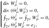 (46)
(46)where \(\{e_j\}_{j=1,\ldots ,d}\) is the standard basis in \({\mathbb {R}}^d\).
- (b)
For every \(k \in {\mathbb {N}}\) and \(r \in [1,\infty ]\)
$$\begin{aligned} \begin{aligned} \Vert D^k \Theta _\mu ^j\Vert _{L^r({\mathbb {T}}^d)}&\le M_{k}\, \mu ^{a + k - (d-1) /r}, \\ \Vert D^k W_\mu ^j\Vert _{L^{r}({\mathbb {T}}^d)}&\le M_{k}\, \mu ^{b + k - (d-1)/r}, \end{aligned} \end{aligned}$$(47)where \(M_{k}\) is a constant which depends only on k, but not on r and \(\mu \).
- (c)
For \(j \ne k\), \(\mathrm {supp} \ \Theta _\mu ^j = \mathrm {supp} \ W_\mu ^j\) and \(\mathrm {supp} \ \Theta _\mu ^j \cap \mathrm {supp} \ W_{\mu }^k = \emptyset \).

We now define the constant M in the statement of Proposition 4.1 as
and we choose
in Proposition 5.1. In this way for each direction \(j =1,\ldots , d\), we obtain a family of Mikado densities \(\{\Theta _\mu ^j\}_{\mu > 2d}\) and fields \(\{W_\mu ^j\}_{\mu >2d}\), obeying the following estimates:
and
and
5.2 Definition of the perturbations
We are now in a position to define \(\rho _1\), \(u_1\). The constant M has already been fixed in (48). Let thus \(p \in [1, d-1)\), \(\eta , \delta >0\) and \((\rho _0, u_0, R_0)\) be a smooth solution to the continuity-defect equation (38).
Let
be parameters, which will be fixed later. Set
For every \(i=1,2,\ldots , N\), let \(I_i := [i\tau , (i+1)\tau ]\) and let \(t_i := (i+1/2)\tau \) be the midpoint of \(I_i\). Consider a partition of unity \(\{\zeta _i\}_{i=1,\ldots , N}\) subordinate to the family of intervals \(\{I_i\}_{i=1,\ldots , N}\). More precisely, for every \(i=1,\ldots , N\), \(\zeta _i \in C^\infty ([0,1])\) and
\(\mathrm {supp} \ \zeta _i \in [(i-1/3)\tau , (i+1+1/3)\tau ]\);
\(\zeta _i (t) \in [0,1]\) for every \(t \in [0,1]\);
\(\sum _{i=1}^N \zeta _i^2(t) = 1\) for every \(t \in [0,1]\).
Notice that for every time \(t \in [0,1]\) there is at most one odd index \(i_1\) and one even index \(i_2\) so that \(\zeta _i(t) = 0\) for every \(i \ne i_1, i_2\). For every \(i=1,\ldots , N\), let \(\Phi _i : [0,1] \times {\mathbb {T}}^d \rightarrow {\mathbb {T}}^d\) be the solution to
i.e. the inverse flow map associated to the vector field \(u_0\), starting at time \(t_i\). Notice that, for fixed t, \(\Phi _i(t) : {\mathbb {T}}^d \rightarrow {\mathbb {T}}^d\) is a measure-preserving diffeomorphism.
We denote by \(R_{0,j}\) the components of \(R_0\), i.e.
Let also \(\psi : [0,1] \rightarrow {\mathbb {R}}\) be a smooth function such that \(\psi (t) \in [0,1]\) for every \(t \in [0,1]\) and
We set
where \(\vartheta , \vartheta _c, w\) are defined as follows. First of all, let \(\Theta _\mu ^j\), \(W_\mu ^j\), \(j=1,\ldots , d\), be the family (depending on \(\mu \)) of Mikado densities and fields provided by Proposition 5.1, with a, b chosen as in (49). We set

The factor \((D \Phi _i(t,x))^{-1}\) is the inverse matrix of \(D \Phi _i(t,x)\). Observe that for fixed \(t_0 \in [0,1]\), there are at most one odd index \(i_1\) and one even index \(i_2\) so that \(\zeta _i(t) =0\) if \(i \ne i_1, i_2\) and t is close enough to \(t_0\) (say, \(|t - t_0| \le 2\tau /3\)). Therefore for such times t we can write
which we will call the fixed-time form of the perturbations. Notice that \(\vartheta \) and w are smooth functions. Notice also that \(\vartheta + \vartheta _c\) has zero mean value in \({\mathbb {T}}^d\) at each time t. Finally observe that w is a sum of terms of the form \((D \Phi )^{-1} G( \Phi )\), with
Since \(\text {div }(W_{\mu })_\lambda = 0\) for every \(\mu , \lambda \) (see Proposition 5.1), we get from Lemma 3.2 that each one of these terms is divergence free and thus \(\text {div }w = 0\). Therefore
Remark 5.2
Observe that, thanks to the cutoff in time \(\psi \), if \(R_0(t) \equiv 0\), then
5.3 Estimates on the perturbation
In this section we estimate \(\vartheta \), \(\vartheta _c\), w.
Lemma 5.3
(\(L^1\)-norm of \(\vartheta \)). For every time \(t \in [0,1]\),
Proof
Since we have to estimate \(\Vert \vartheta (t)\Vert _{L^1({\mathbb {T}}^d)}\) for every fixed time t, we can assume that \(\vartheta (t)\) has the form (56). In (56) each term in the summation over j has the form \(f \cdot (g_\lambda \circ \Phi )\), with
Therefore we can apply the improved Hölder inequality, Lemma 3.4, to get
\(\square \)
Lemma 5.4
(Estimate on \(\vartheta _c\)). For every time \(t \in [0,1]\),
Proof
As in the proof of Lemma 5.3, we can use for \(\vartheta (t)\) the form (56) and we observe that each term in the summation over j has the form \(f \cdot (g_\lambda \circ \Phi )\), with \(f,\Phi ,g, \lambda \) as in (57). We can thus apply Lemma 3.9 to get:
\(\square \)
Lemma 5.5
(\(C^0\) norm of w). For every time \(t \in [0,1]\),
Proof
As in the proof of Lemma 5.3 we can use for w(t) the form (56). Therefore
which is what we wanted to prove.
Lemma 5.6
(\(W^{1,p}\) norm of w). For every time \(t \in [0,1]\),
Proof
As in the proof Lemma 5.5 we can use for w(t) the form (56). Taking one partial derivative \(\partial _k\), we get
We now apply the classical Hölder inequality to estimate \(\Vert \partial _k w(t)\Vert _{L^{p}}\):
A similar (and even easier) computation holds for \(\Vert w(t)\Vert _{L^{p}}\), thus concluding the proof of the lemma.
6 The new defect field
In this section we continue the proof of Proposition 4.1, defining the new defect field \(R_1\) and estimating it.
6.1 Definition of the new defect field
We want to define \(R_1\) so that
Let us compute
where we put
and \(R^{\mathrm{interaction}}\), \(R^{\mathrm{flow}}\), \(R^{\psi }\), \(R^\mathrm{quadr}\), \(R^{\mathrm{transport}}\) will be defined respectively in (63), (64), (65), (66), (70) in such a way that
We thus define
so that (58) holds.
6.2 Definition and estimates for \(R^{\mathrm{interaction}}, R^{\mathrm{flow}}, R^{\psi }, R^{\mathrm{quadr}}\)
In this section we define and estimate the vector fields \(R^\mathrm{quadr}\), \(R^{\mathrm{interaction}}\), \(R^\psi \) and \(R^{\mathrm{flow}}\) so that (61a) holds. First of all, we want to compute more explicitly \(\text {div }(\vartheta (t)w(t) - R_0(t))\), for every fixed time t. We can use the form (56) for \(\vartheta (t)\) and w(t). Exploiting the fact that for \(j \ne k\), \(\Theta _{\mu }^j\) and \(W_{\mu }^k\) have disjoint support (see Proposition 5.1), we have
where we set
On the other side, using the fact that \(\sum _{i=1}^N \zeta _i^2 \equiv 1\), we can write
where we set
with \(\mathrm{Id}\) being the identity matrix, and
Summarizing, we have
where in the last equality we used the fact that \(\text {div }((\Theta _\mu ^j)_\lambda (W_\mu ^j)_\lambda - e_j) = 0\) for every \(\mu , \lambda , j\) (see Proposition 5.1) and Lemma 3.2. We now observe that each term in the two summations over j has zero mean value (being a divergence) and it has the form \(f (D \Phi )^{-1} (g_\lambda \circ \Phi )\), for
We can therefore apply Lemma 3.6 and define
so that (61a) holds. We now separately estimate \(R^\mathrm{interaction}\), \(R^{\mathrm{flow}}\), \(R^{\psi }\), \(R^{\mathrm{quadr}}\). We start with \(R^{\mathrm{interaction}}\).
Lemma 6.1
For every time t it holds
Proof
Consider the definition (63) of \(R^\mathrm{interaction}\). We start by estimating \(\Vert \Theta _{\mu '}^j (\lambda ' \Phi _{i_1}(t))\Vert _{C^1}\) and \(\Vert W_{\mu '}^k(\lambda ' \Phi _{i_1}(t))\Vert _{C^1}\), using (52) and the chain rule
We now estimate \(\Theta _{\mu '}^j (\lambda ' \Phi _{i_1}(t) ) W_{\mu ''}^k (\lambda '' \Phi _{i_2}(t) )\), using the improved Hölder inequality, Lemma 3.4 and considering \(\lambda ''\) as the fast oscillation. We have
where in the last inequality we used (50), (51) and (67). A similar estimate holds for \(\Theta _{\mu ''}^j (\lambda '' \Phi _{i_2}(t)) W_{\mu '}^k (\lambda ' \Phi _{i_1}(t))\):
Therefore
\(\square \)
Lemma 6.2
For every \(t \in [0,1]\),
Proof
The proof follows immediately from the definition of \(R^{\mathrm{flow}}\).
Lemma 6.3
For every \(t \in [0,1]\),
Proof
If \(\psi ^2(t) \ne 1\), then, by (54), \(\Vert R_0(t)\Vert _{L^1} \le \delta /4\) and thus the conclusion follows.
Lemma 6.4
For every \(t \in [0,1]\),
Proof
\(R^{\mathrm{quadr}}(t)\) is defined in (66) using Lemma 3.6. Applying the bounds provided by such proposition, with \(k=0\) and \(p=1\), we get
thus concluding the proof of the lemma.
6.3 Definition and estimates for \(R^{\mathrm{transport}}\)
In this section we define and estimate the vector fields \(R^\mathrm{transport}\) so that (61b) holds. First of all, we want to compute more explicitly \(\partial _t (\vartheta (t) + \vartheta _c(t)) + \text {div }((\vartheta (t)+\vartheta _c(t)) u_0(t))\), for every fixed time t. We can use the fixed-time form (56) for \(\vartheta (t)\) and w(t). We have
where
and we used (53). Here we used the notation \(\dot{f} = df/dt\), if \(f=f(t)\) is a function depending only on time. We now continue the chain of equalities in (68), by adding and subtracting the mean value of each term in the summations over j, as follows:

The last equality is a consequence of the fact that

We now observe that, at the fixed time t, each term in the last line in (69) has the form  for
for
Since \(\Theta _\mu ^j\) has zero mean value (see Proposition 5.1), we can apply Lemma 3.6 and define

Lemma 6.5
For every \(t \in [0,1]\), it holds
Proof
First of all, we observe that
Therefore
We defined \(R^{\mathrm{transport}}\) in (70) using the antidivergence operator provided by Lemma 3.6. We can thus apply the bounds provided by such proposition, with \(k=0\) and \(p=1\), to get
where in the last line we used (50).
6.4 Estimates for \(R^{\mathrm{Nash}}\) and \(R^{\mathrm{corr}}\)
In this section we estimate \(R^{\mathrm{Nash}}\) and \(R^{\mathrm{corr}}\).
Lemma 6.6
For every \(t \in [0,1]\),
Proof
We have
\(\square \)
Lemma 6.7
For every \(t \in [0,1]\),
Proof
We use Lemma 5.4 and Lemma 5.5:
\(\square \)
7 Proof of Proposition 4.1
In this section we conclude the proof of Proposition 4.1, and thus also the proof of Theorem 1.2 and, consequently, the proof of Theorem 1.1. We first prove that if \(R_0(t) = 0\) at some time \(t \in [0,1]\), then \(R_1(t) = 0\). Observe that if \(R_0(t) = 0\), then by Remark 5.2,
Moreover, by (54), \(\psi \equiv 0\) on a neighborhood of t and thus \(\psi (t) = \psi '(t) = 0\). Therefore
and thus \(R_1(t) = 0\).
We now prove estimates (39a)–(39d). First of all, in view of Lemma 5.5 and Lemma 6.2, we choose \(\tau \) so small that
This is always possible since, by (53), \(\Phi _i(t_i, x) = x\) and thus \(D \Phi _i(t_i, x) = \mathrm{Id}\) for every \(i=1,\ldots , N\). We choose also \(\lambda ', \mu ', \lambda '', \mu ''\) such that \(1 \ll \lambda ' \ll \mu ' \ll \lambda '' \ll \mu ''\). More precisely, we set
for some
and \(\lambda \gg 1\) to be fixed later.
1 Estimate (39a). If \(R_0(t) = 0\), we have already seen that \(\rho _1(t) = \rho _0(t)\). We can thus assume \(R_0(t) \ne 0\). We have
if the constant \(\lambda \) is chosen large enough.
2 Estimate (39b). We have
3 Estimate (39c). We have
if \(\alpha \), \(\beta , \gamma \) are chosen so that
and \(\lambda \) is large enough.
4 Estimate (39d). Recall the definition of \(R_1\) in (62). Using Lemmas 6.1, 6.2, 6.3, 6.4, 6.5, 6.6, 6.7 and (71b), we get
if
and \(\lambda \) is large enough.
We still have to choose \(\alpha , \beta , \gamma \) so that (72), (73) are satisfied. This can be easily done as follows, recalling that \(p < d-1\). First we fix \(\alpha > 1\) so that
so that (72a) is satisfied. Then we choose \(\beta \) so that
so that (73a) is satisfied. Finally we choose \(\gamma >1\) so that
so that (72b) and (73b) are satisfied. This concludes the proof of Proposition 4.1 and thus also the proof of Theorem 1.2 and, consequently, the proof of Theorem 1.1.
Notes
While the present paper was under review, G. Sattig and the first author, relying on the ideas introduced in the present paper, showed in [15] that this dimensional threshold can be raised up to d.
References
Ambrosio, L.: Transport equation and Cauchy problem for BV vector fields. Invent. Math. 158(2), 227–260 (2004)
Ambrosio, L.: Well posedness of ODE’s and continuity equations with nonsmooth vector fields, and applications. Rev. Mat. Complut. 30(3), 427–450 (2017)
Bianchini, S., Bonicatto, P.: A uniqueness result for the decomposition of vector fields in Rd. SISSA (2017)
Buckmaster, T., De Lellis, C., Isett, P., Székelyhidi Jr., L.: Anomalous dissipation for 1/5-Hölder Euler flows. Ann. Math. (2) 182(1), 127–172 (2015)
Buckmaster, T., De Lellis, C., Székelyhidi Jr., L., Vicol, V.: Onsager’s conjecture for admissible weak solutions. Commun. Pure Appl. Math. 72, 229–274 (2019)
Buckmaster, T., Vicol, V.: Nonuniqueness of weak solutions to the Navier–Stokes equation. Ann. Math. (2) 189(1), 101–144 (2019)
Caravenna, L., Crippa, G.: Uniqueness and Lagrangianity for solutions with lack of integrability of the continuity equation. C. R. Math. Acad. Sci. Paris 354(12), 1168–1173 (2016)
Daneri, S., Székelyhidi Jr., L.: Non-uniqueness and h-principle for Hölder-continuous weak solutions of the Euler equations. Arch. Ration. Mech. Anal. 224(2), 471–514 (2017)
De Lellis, C., Székelyhidi Jr., L.: On admissibility criteria for weak solutions of the Euler equations. Arch. Ration. Mech. Anal. 195(1), 225–260 (2008)
Depauw, N.: Non unicité des solutions bornées pour un champ de vecteurs BV en dehors d’un hyperplan. C. R. Math. Acad. Sci. Paris 337(4), 249–252 (2003)
DiPerna, R.J., Lions, P.-L.: Ordinary differential equations, transport theory and Sobolev spaces. Invent. Math. 98(3), 511–547 (1989)
Evans, L.C.: Partial Differential Equations. American Mathematical Society, Providence (2010)
Isett, P.: A proof of Onsager’s conjecture. Ann. Math. (2) 188(3), 871–963 (2018)
Isett, P., Oh, S.-J.: On nonperiodic Euler flows with Hölder regularity. Arch. Ration. Mech. Anal. 221(2), 725–804 (2016)
Modena, S., Sattig, G.: Convex integration solutions to the transport equation with full dimensional concentration. arXiv (2019)
Modena, S., Székelyhidi, L.: Non-uniqueness for the transport equation with Sobolev vector fields. Ann. PDE 4(2), 18 (2018)
Acknowledgements
This research was supported by the ERC Grant Agreement No. 724298.
Author information
Authors and Affiliations
Corresponding author
Additional information
Communicated by L. Ambrosio.
Publisher's Note
Springer Nature remains neutral with regard to jurisdictional claims in published maps and institutional affiliations.
Rights and permissions
Open Access This article is distributed under the terms of the Creative Commons Attribution 4.0 International License (http://creativecommons.org/licenses/by/4.0/), which permits unrestricted use, distribution, and reproduction in any medium, provided you give appropriate credit to the original author(s) and the source, provide a link to the Creative Commons license, and indicate if changes were made.
About this article

Cite this article
Modena, S., Székelyhidi, L. Non-renormalized solutions to the continuity equation. Calc. Var. 58, 208 (2019). https://doi.org/10.1007/s00526-019-1651-8
Received:
Accepted:
Published:
DOI: https://doi.org/10.1007/s00526-019-1651-8