Some Properties of the Potential-to-Ground State Map in Quantum Mechanics

Abstract

We analyze the map from potentials to the ground state in static many-body quantum mechanics. We first prove that the space of binding potentials is path-connected. Then we show that the map is locally weak–strong continuous and that its differential is compact. In particular, this implies the ill-posedness of the Kohn–Sham inverse problem.

Appendices

Appendix A: Basic Inequalities on Potentials

We recall here in LemmaA.1 several well-known facts about potentials.

Lemma A.1

Take $v,w \in (L^p+L^{\infty })(\mathbb {R}^d)$.

• (i) Taking p as in (1), we have

  

  (37)

• (ii) Let $\mathcal {C}\subset \mathbb {C}$, be a contour in the complex plane which is such that ${{\,\mathrm{dist}\,}}\left( z,\sigma (H_N(v)) \right) \geqslant \eta > 0$ uniformly in $z \in \mathcal {C}$. Let p be as in (1), then the operators

  $$\begin{aligned} \left( -\Delta +1 \right) ^{-\frac{1}{2}} \big ( H_N-z \big ) \left( -\Delta +1 \right) ^{-\frac{1}{2}}, \,\,\,\,\,\,\,\,\,\left( -\Delta +1 \right) ^{\frac{1}{2}} \big ( H_N-z \big )^{-1}\left( -\Delta +1 \right) ^{\frac{1}{2}} \end{aligned}$$

  are uniformly bounded in $z \in \mathcal {C}$.

• (iii) Let $v \in \mathcal {V}_N^{(0)}$, and p as in (1). For $u \in L^p+L^{\infty }$ such that $\left| \! \left| u \right| \! \right| _{L^p+L^{\infty }}$ is small enough, we have $v+u \in \mathcal {V}_N^{(0)}$.

Proof

(i) $\bullet$  If p is as in (1), we have

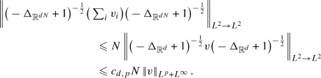
where we used that $\left| \! \left| (-\Delta _i)^{\frac{1}{2}} (-\Delta _{\mathbb {R}^{dN}} +1)^{-\frac{1}{2}} \right| \! \right| _{L^2 \rightarrow L^2} =1$.

$\bullet$  Let us write $v = v_p + v_{\infty }$. We have

$$\begin{aligned}&\left| \! \left| \left( -\Delta +1 \right) ^{-\frac{1}{2}}v\left( -\Delta +1 \right) ^{-\frac{1}{2}} \right| \! \right| _{L^2 \rightarrow L^2} \nonumber \\&\quad \leqslant \left| \! \left| \left( -\Delta +1 \right) ^{-\frac{1}{2}}v_p\left( -\Delta +1 \right) ^{-\frac{1}{2}} \right| \! \right| _{L^2 \rightarrow L^2} \nonumber \\&\quad \quad \quad \quad \quad + \left| \! \left| \left( -\Delta +1 \right) ^{-\frac{1}{2}}v_{\infty }\left( -\Delta +1 \right) ^{-\frac{1}{2}} \right| \! \right| _{L^2 \rightarrow L^2}\nonumber \\&\quad \leqslant \left| \! \left| \left( -\Delta +1 \right) ^{-\frac{1}{2}}v_p\left( -\Delta +1 \right) ^{-\frac{1}{2}} \right| \! \right| _{L^2 \rightarrow L^2} + \left| \! \left| v_{\infty } \right| \! \right| _{L^{\infty }} \nonumber \\&\quad \leqslant \left| \! \left| \sqrt{\left| v_p\right| } \left( -\Delta +1 \right) ^{-\frac{1}{2}} \right| \! \right| _{L^2 \rightarrow L^2}^2 + \left| \! \left| v_{\infty } \right| \! \right| _{L^{\infty }} . \end{aligned}$$

(38)

In the last inequality, we used that

$$\begin{aligned} \left( -\Delta +1 \right) ^{-\frac{1}{2}} v_p \left( -\Delta +1 \right) ^{-\frac{1}{2}} = \left( -\Delta +1 \right) ^{-\frac{1}{2}} \sqrt{\left| v_p\right| } {{\,\mathrm{sgn}\,}}(v_p) \sqrt{\left| v_p\right| }\left( -\Delta +1 \right) ^{-\frac{1}{2}}, \end{aligned}$$

where ${{\,\mathrm{sgn}\,}}(v)$ is equal to 1 if $v > 0$, $-1$ if $v <0$ and 0 if $v =0$, it satisfies $\left| \! \left| {{\,\mathrm{sgn}\,}}(v) \right| \! \right| _{L^2 \rightarrow L^2} \leqslant 1$, hence

$$\begin{aligned} \left| \! \left| \left( -\Delta +1 \right) ^{-\frac{1}{2}} v_p \left( -\Delta +1 \right) ^{-\frac{1}{2}} \right| \! \right| _{L^2 \rightarrow L^2} \leqslant \left| \! \left| \sqrt{\left| v_p\right| } \left( -\Delta +1 \right) ^{-\frac{1}{2}} \right| \! \right| _{L^2 \rightarrow L^2}^2. \end{aligned}$$

As for the first term in (38), for $d \geqslant 3$, with $p = d/2$ we have

$$\begin{aligned} \left| \! \left| \sqrt{\left| v_p\right| } \left( -\Delta +1 \right) ^{-\frac{1}{2}} \right| \! \right| _{L^2 \rightarrow L^2}&\leqslant \left| \! \left| \sqrt{\left| v_p\right| } (-\Delta )^{-\frac{1}{2}} \right| \! \right| _{L^2 \rightarrow L^2} \leqslant c_{d} \left| \! \left| \sqrt{\left| v_p\right| } \right| \! \right| _{L^{2p}} \\&= c_{d} \sqrt{ \left| \! \left| v_p \right| \! \right| _{L^{p}} }, \end{aligned}$$

where we used the Hardy–Littlewood–Sobolev inequality [40, Theorem 4.3] in the last inequality. For $d \in \left\{ 1,2 \right\}$, we can use the Kato–Seiler–Simon inequality [53, Theorem 4.1] to get

$$\begin{aligned} \left| \! \left| \sqrt{\left| v_p\right| } \left( -\Delta +1 \right) ^{-\frac{1}{2}} \right| \! \right| _{L^2 \rightarrow L^2}&\leqslant \left| \! \left| \sqrt{\left| v_p\right| } \left( -\Delta +1 \right) ^{-\frac{1}{2}} \right| \! \right| _{\mathfrak {S}_{2p}} \\&\leqslant (2\pi )^{-d/(2p)} \left| \! \left| \sqrt{\left| v_p\right| } \right| \! \right| _{L^{2p}} \left| \! \left| \big ( \left| x\right| ^2+1 \big )^{-\frac{1}{2}} \right| \! \right| _{L^{2p}} \\&\leqslant c_{d,p} \sqrt{ \left| \! \left| v_p \right| \! \right| _{L^{p}} }. \end{aligned}$$

(ii) Take $c \geqslant 0$ and let us define . We remark that

$$\begin{aligned} H + c = (-\Delta +c)^{\frac{1}{2}} \left( 1+ (-\Delta +c)^{-\frac{1}{2}} A (-\Delta +c)^{-\frac{1}{2}} \right) (-\Delta +c)^{\frac{1}{2}}, \end{aligned}$$

hence we only need to show that $\left| \! \left| (-\Delta +c)^{-\frac{1}{2}} A (-\Delta +c)^{-\frac{1}{2}} \right| \! \right| _{L^2 \rightarrow L^2} <1$. For instance we will show that

$$\begin{aligned} \left| \! \left| (-\Delta _{\mathbb {R}^d} + c)^{-\frac{1}{2}} v (-\Delta _{\mathbb {R}^d} + c)^{-\frac{1}{2}} \right| \! \right| _{L^2 \rightarrow L^2} \leqslant \left| \! \left| \sqrt{\left| v\right| } (-\Delta _{\mathbb {R}^d} + c)^{-\frac{1}{2}} \right| \! \right| _{L^2 \rightarrow L^2}^2 \end{aligned}$$

is as small as we want. For any $\epsilon > 0$, there exists $c_{\epsilon } \geqslant 0$ such that $\left| v\right| \leqslant \epsilon (-\Delta ) + c_{\epsilon }$ in the sense of forms, hence for all $u \in \mathcal {C}^{\infty }$, we have

$$\begin{aligned} \left| \! \left| \sqrt{\left| v\right| } (-\Delta + c)^{-\frac{1}{2}} u \right| \! \right| _{L^2}^2&\leqslant \epsilon \left| \! \left| (-\Delta )^{\frac{1}{2}} (-\Delta + c)^{-\frac{1}{2}} u \right| \! \right| _{L^2}^2 + c_{\epsilon } \left| \! \left| (-\Delta + c)^{-\frac{1}{2}} u \right| \! \right| _{L^2}^2 \\&\leqslant \left( \epsilon + \frac{c_{\epsilon }}{c} \right) \left| \! \left| u \right| \! \right| _{L^2}^2. \end{aligned}$$

We can first choose $\epsilon$ small and then choose c large so that the quantity $\left| \! \left| \sqrt{\left| v\right| } (-\Delta + c)^{-\frac{1}{2}} \right| \! \right| _{L^2 \rightarrow L^2}$ is arbitrarily small.

(iii) The statement follows from the resolvent formula

and Cauchy’s formula

see for instance [36, 50]. $\quad \square$

Appendix B: Weak–Strong Continuity and Compactness

We recall here relations between weak–strong continuity and compactness. Following [23, Definition 7.6], we say that a map is compact if it maps bounded sets into relatively compact sets. The link between ill-posedness of a problem and its linearization can be involved, see for instance [52] and [7, Appendix]. We start by considering standard results, and adapt them to the case when the image space is an embedded submanifold.

Lemma B.1

Let X and Y be Banach spaces, $U \subset X$ an open set, a closed embedded submanifold of Y, and a map $f : U \rightarrow M$.

• (i) If f is compact, continuous and differentiable on U, then $\mathrm{d}_x f$ is compact for any $x \in U$.

• (ii) If $U = X$ is the dual of a Banach space, and if f is weak–strong continuous, then f is compact.

• (iii) If f is compact and M is infinite-dimensional, then f(X) is a countable union of compact sets, and f(X) has empty interior.

• (iv) If f is compact and X is infinite-dimensional, then $f^{-1}$ is discontinuous.

Proof

The only difference in the proof, compared to the case $M=Y$, is (i).

• (i) In the case $M = Y$, this is proved in [23]. We apply it to $\iota _{M \rightarrow Y} \circ f : U \rightarrow Y$ and get that $\mathrm{d}_x \left( \iota _{M \rightarrow Y} \circ f \right) \left( X \cap \left\{ \left| \! \left| \cdot \right| \! \right| _{L^2 \rightarrow L^2} \leqslant 1 \right\} \right) = \iota _{\mathrm{T}_{f(x)} M \rightarrow Y} \circ \left( \mathrm{d}_x f \right) \left( X \cap \left\{ \left| \! \left| \cdot \right| \! \right| _{L^2 \rightarrow L^2} \leqslant 1 \right\} \right)$ is compact. A map is proper if preimages of relatively compact open sets are relatively compact open sets [56, Definition 16.26]. One can prove that for a Banach space F and a closed subset $E \subset F$, the inclusion map is proper. Since $\iota _{\mathrm{T}_{f(x)} M \rightarrow Y}$ is proper, then $\left( \mathrm{d}_x f \right) \left( X \cap \left\{ \left| \! \left| \cdot \right| \! \right| _{L^2 \rightarrow L^2} \leqslant 1 \right\} \right)$ is relatively compact. We remark that we only used that is an embedded submanifold of Y, we did not use the closed condition.

• (ii) Let $G \subset B_0(r) \subset X$ be a bounded set and $x_n \in G$ a sequence. By Banach–Alaoglu’s theorem, $x_n \rightharpoonup x$ for some $x \in B_0(r)$ and up to a subsequence. By weak–strong continuity of f, $f(x_n) \rightarrow f(x)$ strongly.

• (iii) We define the sets $X_r :=X \cap \left\{ x \in X \, \bigr \vert \, \left| \! \left| x \right| \! \right| _{X} \leqslant r \right\}$, for $r \geqslant 0$. Since f is compact, then the $\overline{f(X_r)}$’s are compact and thus have empty interiors by Riesz’s theorem [4, Theorem 6.5], which applies in our case because M is locally a normed vector space. We have

  $$\begin{aligned} f(X) = \cup _{r\in \mathbb {N}} f(X_r) \subset \cup _{r\in \mathbb {N}} \overline{f(X_r)}. \end{aligned}$$

  Finally, by Baire’s theorem [4, Theorem 2.1] f(X) has empty interior. We recall that a closed subset of a compact space is compact.

• (iv) Let $B \subset X$ be a ball, f(B) is relatively compact. Assuming that $f^{-1}$ is continuous, $f^{-1}\left( f(B) \right) \supset B$, is also relatively compact, and hence B as well. But this contradicts [4, Theorem 6.5]. The inverse $f^{-1}$ is thus discontinuous.

$\square$

Here is a summary of the relations between compactness and weak–strong continuity for a map and its differential.

We also remark that $\mathrm{d}_x f$ weak–strong continuous for any $x \in U$ does not imply that f is weak–strong continuous, a simple counterexample is $L^2(\mathbb {R}^n) \ni x \mapsto \left| \! \left| x \right| \! \right| _{L^2}^2$, and this is also the case for $v \mapsto \Psi (v)$.

References

Abraham, R., Marsden, J.E., Ratiu, T.: Manifolds, Tensor Analysis, and Applications, vol. 75. Springer, New York (2012)
Agmon, S.: Lectures on Exponential Decay of Solutions of Second-Order Elliptic Equations. Princeton University Press, Princeton (1982)
Bach, V., Delle Site, L.: On some open problems in many-electron theory. In: Bach, V., Delle Site, L. (eds.) Many-Electron Approaches in Physics, Chemistry and Mathematics. Mathematical Physics Studies, pp. 413–417. Springer, New York (2014)
Brezis, H.: Functional Analysis, Sobolev Spaces and Partial Differential Equations. Springer, New York (2010)
Courant, R., Hilbert, D.: Methods of Mathematical Physics: Partial Differential Equations. Wiley, New York (2008)
Cwikel, M.: Weak type estimates for singular values and the number of bound states of Schrödinger operators. Ann. Math. 106, 93–100 (1977)
Engl, H.W., Kunisch, K., Neubauer, A.: Convergence rates for Tikhonov regularisation of non-linear ill-posed problems. Inverse Probl. 5, 523 (1989)
Feynman, R.P.: Forces in molecules. Phys. Rev. 56, 340 (1939)
Garrigue, L.: Unique continuation for many-body Schrödinger operators and the Hohenberg–Kohn theorem. Math. Phys. Anal. Geom. 21, 27 (2018)
Garrigue, L.: Hohenberg–Kohn theorems for interactions, spin and temperature. J. Stat. Phys. (2019)
Garrigue, L.: Unique continuation for many-body Schrödinger operators and the Hohenberg–Kohn theorem. II. The Pauli Hamiltonian, Doc. Math. (2020)
Garrigue, L.: Building Kohn–Sham potentials for ground and excited states. arXiv e-prints arXiv:2101.01127 (2021)
Gaudoin, R., Burke, K.: Lack of Hohenberg–Kohn theorem for excited states. Phys. Rev. Lett. 93, 173001 (2004)
Güttinger, P.: The behavior of atoms in a rotating magnetic field. Z. Phys. 73, 169–184 (1932)
Hadamard, J.: Le problème de Cauchy et les équations aux dérivées partielles linéaires hyperboliques, vol. 220. Paris Russian translation (1932)
Hadamard, J.: La théorie des équations aux dérivées partielles, Éditions scientifiques (1964)
Hainzl, C., Lewin, M., Séré, É.: Self-consistent solution for the polarized vacuum in a no-photon QED model. J. Phys. A 38, 4483–4499 (2005)
Harriman, J.E.: Orthonormal orbitals for the representation of an arbitrary density. Phys. Rev. A 24, 680–682 (1981)
Hasanoğlu, A.H., Romanov, V.G.: Introduction to Inverse Problems for Differential Equations. Springer, New York (2017)
Hellman, H.: Einführung in die quantenchemie, vol. 285. Franz Deuticke, Leipzig (1937)
Hirschfelder, J.O.: Formal Rayleigh–Schrödinger perturbation theory for both degenerate and non-degenerate energy states. Int. J. Quantum Chem. 3, 731–748 (1969)
Hislop, P.: Exponential decay of two-body eigenfunctions: a review. In: Proceedings of the Symposium on Mathematical Physics and Quantum Field Theory (Berkeley, CA, 1999), vol. 4, pp. 265–288 (2000)
Hohage, T.: Lecture Notes on Inverse Problems (2002)
Hohenberg, P., Kohn, W.: Inhomogeneous electron gas. Phys. Rev. 136, B864–B871 (1964)
Hunziker, W.: On the spectra of Schrödinger multiparticle Hamiltonians. Helv. Phys. Acta 39, 451–462 (1966)
Ismail, M.E., Zhang, R.: On the Hellmann–Feynman theorem and the variation of zeros of certain special functions. Adv. Appl. Math. 9, 439–446 (1988)
Jerison, D., Kenig, C.E.: Unique continuation and absence of positive eigenvalues for Schrödinger operators. Ann. Math. 121, 463–494 (1985) (With an appendix by E. M. Stein)
Kato, T.: On the convergence of the perturbation method. Prog. Theor. Phys. 5, 207–212 (1950)
Kato, T.: Perturbation Theory for Linear Operators, 2nd edn. Springer, New York (1995)
Kohn, W., Sham, L.J.: Self-consistent equations including exchange and correlation effects. Phys. Rev. 2(140), A1133–A1138 (1965)
Lampart, J.: A remark on the attainable set of the Schrödinger equation. Evol. Equ. Control Theory (2020)
Lang, S.: Differential Manifolds, vol. 212. Springer, New York (1972)
Lewin, M.: A mountain pass for reacting molecules. Ann. Henri Poincaré 5, 477–521 (2004)
Lewin, M.: Describing lack of compactness in Sobolev spaces. Lecture-taken from unpublished lecture notes "Variational Methods in Quantum Mechanics" written for a course delivered at the University of Cergy–Pontoise in 2010 (2010)
Lewin, M.: Geometric methods for nonlinear many-body quantum systems. J. Funct. Anal. 260, 3535–3595 (2011)
Lewin, M.: Théorie spectrale & mécanique quantique. Cours de l’École polytechnique (2018)
Lieb, E.H.: Density functionals for Coulomb systems. Int. J. Quantum Chem. 24, 243–277 (1983)
Lieb, E.H.: On the lowest eigenvalue of the Laplacian for the intersection of two domains. Invent. Math. 74, 441–448 (1983)
Lieb, E.H.: The Number of Bound States of One-Body Schrödinger Operators and the Weyl Problem, in The Stability of Matter: From Atoms to Stars, pp. 241–252. Springer, New York (1997)
Lieb, E.H., Loss, M.: Analysis. Graduate Studies in Mathematics, vol. 14, 2nd edn. American Mathematical Society, Providence (2001)
Lieb, E.H., Simon, B.: The Thomas–Fermi theory of atoms, molecules and solids. Adv. Math. 23, 22–116 (1977)
Lions, P.-L.: The concentration-compactness principle in the calculus of variations. The locally compact case, Part I. Ann. Inst. H. Poincaré Anal. Non Linéaire 1, 109–149 (1984)
Lions, P.-L.: The concentration-compactness principle in the calculus of variations. The locally compact case, Part II. Ann. Inst. H. Poincaré Anal. Non Linéaire 1, 223–283 (1984)
Lions, P.-L.: The concentration-compactness principle in the calculus of variations. The limit case I. Rev. Mat. Iberoamericana 1, 145–201 (1985)
Lions, P.-L.: The concentration-compactness principle in the calculus of variations. The limit case II. Rev. Mat. Iberoamericana 1, 45–121 (1985)
Perdew, J.P., Parr, R.G., Levy, M., Balduz, J.L., Jr.: Density-functional theory for fractional particle number: derivative discontinuities of the energy. Phys. Rev. Lett. 49, 1691 (1982)
Pflaum, M.J.: The geometry of classical and quantum fields (2019)
Ray, W.O., Walker, A.M.: Mapping theorems for Gateaux differentiable and accretive operators. Nonlinear Anal. Theor. 6, 423–433 (1982)
Reed, M., Simon, B.: Methods of Modern Mathematical Physics I. Functional Analysis. Academic Press, New York (1972)
Reed, M., Simon, B.: Methods of Modern Mathematical Physics IV. Analysis of Operators. Academic Press, New York (1978)
Rozenbljum, G.: Distribution of the discrete spectrum of singular differential operators. Soviet Math. Doki. 202, 1012–1015 (1972)
Schock, E.: Non-linear ill-posed equations: counter-examples. Inverse Probl. 18, 715–717 (2002)
Simon, B.: Trace Ideals and Their Applications. London Mathematical Society Lecture Note Series, vol. 35. Cambridge University Press, Cambridge (1979)
Simon, B.: Schrödinger semigroups. Bull. Am. Math. Soc. (N.S.) 7, 447–526 (1982)
Simon, B.: A Comprehensive Course in Analysis, Part 4: Operator Theory. American Mathematical Society, Providence (2015)
Souriau, J.-M.: Structure of Dynamical Systems: A Symplectic View of Physics, vol. 149. Springer, New York (2012)
Struwe, M.: Variational Methods: Applications to Nonlinear Partial Differential Equations and Hamiltonian Systems, 4th edn. Springer, New York (2008)
Teufel, S.: Adiabatic Perturbation Theory in Quantum Dynamics. Lecture Notes in Mathematics, vol. 1821. Springer, Berlin (2003)
Van Winter, C.: Theory of finite systems of particles. I. The Green function. Mat.-Fys. Skr. Danske Vid. Selsk. 2 (1964)
Weinberg, S.: The Quantum Theory of Fields, vol. I. Cambridge University Press, Cambridge (1996)
Zeidler, E.: Nonlinear Functional Analysis and Its Applications. I: Fixed-Point Theorems, vol. 1. Springer, New York (1985)
Zeidler, E.: Nonlinear Functional Analysis and Its Applications IV, Applications to Mathematical Physics. Springer, New York (2013)
Zhislin, G.M.: A study of the spectrum of the Schrödinger operator for a system of several particles. Trudy Moskov. Mat. Obšč. 9, 81–120 (1960)
Acknowledgements
I warmly thank Mathieu Lewin, my PhD director, for having advised me during this work. This project has received funding from the European Research Council (ERC) under the European Union’s Horizon 2020 research and innovation programme (grant agreement MDFT No 725528).
Author information
Authors and Affiliations
Corresponding author
Additional information
Communicated by A. Giuliani
Publisher's Note
Springer Nature remains neutral with regard to jurisdictional claims in published maps and institutional affiliations.