Quasiconvexity, Null Lagrangians, and Hardy Space Integrability Under Constant Rank Constraints

Abstract

We present a systematic treatment of the theory of Compensated Compactness under Murat’s constant rank assumption. We give a short proof of a sharp weak lower semicontinuity result for signed integrands, extending aspects of the results of Fonseca–Müller. The null Lagrangians are an important class of signed integrands, since they are the weakly continuous functions. We show that they are precisely the compensated compactness quantities with Hardy space integrability, thus proposing an answer to a question raised by Coifman–Lions–Meyer–Semmes. Finally we provide an effective way of computing the null Lagrangians associated with a given operator.

1 Introduction

Let $\mathcal A$ be a linear partial differential operator acting on fields $v:\mathbb {R}^n\rightarrow \mathbb V$, for some finite-dimensional inner product space $\mathbb V$. In this paper, we address the following question:

Main question. Are there special quantities $F:\mathbb V \rightarrow \mathbb {R}$ which are well-behaved with respect to solutions of the system $\mathcal A v=0$? In particular:

• For solutions of $\mathcal A v=0$, does F(v) benefit from compensated regularity?, e.g.

  $$\begin{aligned} v\in C^\infty _{c}(\mathbb {R}^n, \mathbb V) and \,\mathcal A v=0 \implies F(v)\in \mathscr {H}^1(\mathbb {R}^n). \end{aligned}$$

  (1.1)

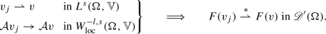
• For solutions of $\mathcal A v=0$, does F(v) benefit from compensated compactness?, e.g.

  $$\begin{aligned} v_j\overset{*}{\rightharpoonup }v in L^\infty _loc (\mathbb {R}^n,\mathbb V) and \mathcal A v_j=0 \implies F(v_j)\overset{*}{\rightharpoonup }F(v) in \mathscr {D}'(\mathbb {R}^n). \end{aligned}$$

  (1.2)

If there are such quantities, how do we characterize and compute them?

It is clear that, for the first part, one should look for nonlinear quantities, since otherwise F(v) has precisely the same regularity as v. In (1.1), $\mathscr {H}^1(\mathbb {R}^n)$ denotes the real Hardy space, which can be thought of as a proper subspace of $L^1(\mathbb {R}^n)$ whose elements have cancellations at all scales, and therefore have additional integrability. Being able to identify $L^1$-quantities that in fact have Hardy space integrability is often important in PDE: this has been useful in Fluid Dynamics [33,34,35] as well as Differential Geometry [51, 79] and we refer the reader to [18] for further examples and references.

Weakly continuous functions, as in (1.2), can be thought of as representing physical quantities that are robust to errors in measurements induced from small-scale oscillations. We call these quantities null Lagrangians [7] or $\mathcal A$-quasiaffine functions [23] and they are the classical objects of study in the Murat–Tartar theory of Compensated Compactness [81, 82, 99, 100]. In the last four decades, the theory was developed much further, having found applications in Continuum Mechanics [31,32,33], Homogenization [11, 15, 73, 74] and Nonlinear Analysis [4, 29, 42, 58, 80]. We also refer the reader to the recent papers [3, 21, 25, 85].

The two main contributions of our work are as follows: under standard assumptions in compensated compactness theory, we show that (1.1) and (1.2) are equivalent; we also give a comprehensive treatment of (1.2) and its generalizations. The former gives an answer to a question of Coifman–Lions–Meyer–Semmes raised in [18], whereas the latter improves aspects of the classical work of Murat–Tartar [82] and Fonseca–Müller [43]. The main novelty of this paper is an enhanced version of the tools introduced by the second author in [87], which make our proofs very clear and streamlined. We expect our ideas to be useful for different problems, see the recent developments in [64, 66].

To be precise, in our main question we consider an operator $\mathcal A$ of the form

$$\begin{aligned} \mathcal A=\sum _{|\alpha |=l} A_\alpha \partial ^\alpha , \qquad where A_\alpha \in Lin (\mathbb V, \mathbb W) \end{aligned}$$

for some finite dimensional inner product spaces $\mathbb V,\mathbb W$. The prototypical example we have in mind is $\mathcal A(B,E)=(div \, B, curl \,E)$, for a domain $\Omega \subset \mathbb {R}^n$ and fields $E,\,B:\Omega \rightarrow \mathbb {R}^{n}$ in $L^2(\Omega )$, which we think of as the electric and the magnetic fields respectively. Coifman–Lions–Meyer–Semmes [18] proved that (1.1) holds, i.e.,

$$\begin{aligned} div \,B=0, curl\, E=0 \quad \implies \quad B\cdot E\in \mathscr {H}^1(\mathbb {R}^n).\end{aligned}$$

(1.3)

The implication (1.3) was inspired by a surprising and remarkable result of Müller [76] and it can be proved through the Coifman–Rochberg–Weiss commutator theorem [19], see also [67] for a different approach and [24] for local, non-homogeneous versions. The quantity $E\cdot B$ is also weakly continuous for the system $(div , curl )$, a fact which goes back to the pioneering work of Murat and Tartar [99]: if $d=n^2+1$, then (1.2) holds, i.e.,

(1.4)

Continuum Mechanics furnishes plenty of interesting examples beyond electromagnetism: in the theory of elasticity the deformation gradient is irrotational, while the linearized strain satisfies the Saint-Venant compatibility condition, and in incompressible fluid flow the velocity field is divergence-free; see also Example 3.8. In these examples the operator $\mathcal A$ has an important non-degeneracy property:

$$\begin{aligned} \mathcal {A} has constant rank and span \, \Lambda _{\mathcal A}=\mathbb V. \end{aligned}$$

(1.5)

Here $\Lambda _{\mathcal A}$ is the wave cone of the operator $\mathcal A$, see also Section 3 for notation and terminology, and the spanning assumption is natural since weakly continuous quantities are completely unconstrained along directions not in $span \, \Lambda _\mathcal A$. The constant rank assumption is standard [43, 82] and, per the results of the authors in [48], it is equivalent to a certain $L^p$-estimate on which many results in compensated compactness theory crucially rely. In the constant rank case, weak continuity is well understood since Murat’s work [82] but, without this assumption, very little is known, an important exception being the case of separate convexity [77, 101], which was proposed by Tartar as a toy model for rank-one convexity. The case of quadratic functions F is also special: in this setting, there is a satisfactory theory both for Hardy integrability [18, 68] and for weak continuity [99]. However, these proofs rely crucially on Plancherel’s Theorem.

Returning to the div-curl example, we observe that the inner product is both weakly continuous and has Hardy space integrability. Hence, the following natural question was asked in [18]: is this a general phenomenon, i.e. is it the case that (1.1) and (1.2) are equivalent? Our main theorem shows that, under the standard assumption (1.5), this is indeed the case.

Theorem A

(Hardy integrability $\iff$ weak continuity) Assume (1.5) and let $F:\mathbb V\rightarrow \mathbb {R}$ be a locally bounded, Borel function that is not affine. Then (1.1) holds if and only if (1.2) holds and in that case we have:

• F is a polynomial of degree $s\leqq \min \{n,\dim \mathbb V\}$ and it is $\mathcal A$-quasiaffine, i.e. F and $-F$ are both $\mathcal A$-quasiconvex;

• if moreover F is homogeneous, there is an estimate

  $$\begin{aligned} \Vert F(v)\Vert _{\mathscr {H}^1(\mathbb {R}^n)}&\leqq C\Vert v \Vert _{L^s(\mathbb {R}^n)} \qquad for all v\in L^s(\mathbb {R}^n) with \mathcal A v=0 in \mathscr {D}'(\mathbb {R}^n). \end{aligned}$$

The class of such polynomials can be computed explicitly by solving an algebraic system of linear equations.

Theorem A shows that compensated compactness and compensated regularity are two facets of the algebraic cancellations in the nonlinearity, which compensate the lack of ellipticity of the operator $\mathcal A$.

When F is linear, it is possible to make a statement similar to the one in Theorem A, c.f. Theorem 6.1, although we show that there is no estimate in that case. We would also like to highlight that we provide an effective way of computing the $\mathcal A$-quasiaffine functions. Murat [82] derived the algebraic identity (5.4) that characterizes these functions but, as he was already aware, it is in general not feasible to decide which nonlinear polynomials, if any, satisfy this identity. In order to deal with this issue, we crucially rely on the work of Ball–Currie–Olver [5]. We deduce that all $\mathcal A$-quasiaffine functions can be written as coefficients of differential forms, which answers in the positive a question of Robbin–Rogers–Temple [90, §5] under the assumption (1.5). Our main new tool is an $L^p$ Helmholtz–Hodge decomposition for constant rank operators, which is based on the existence of potential operators. These were constructed recently by the second author in [87].

In the setup of Theorem A, it is natural to wonder whether the convergence in (1.2) can be improved. Tartar [102, Lemma 7.3] showed that one cannot upgrade weak-$*$ convergence in measures to weak convergence in $L^1$, i.e. one cannot test the convergence against $L^\infty$ functions. However, as a by product of Theorem A, one can test the convergence against functions in $VMO (\mathbb {R}^n)$; this a space which is neither contained nor contains $L^\infty (\mathbb {R}^n)$.

Theorem B

(Improved and quantified convergence) As before assume (1.5) and let $F:\mathbb V\rightarrow \mathbb {R}$ be $\mathcal A$-quasiaffine and s-homogeneous for some $s\geqq 2$. Then

$$\begin{aligned} v_j \rightharpoonup v in L^s(\mathbb {R}^n,\mathbb V) and \mathcal A v_j=0\implies F(v_j)\overset{*}{\rightharpoonup }F(v) in \mathscr {H}^1(\mathbb {R}^n). \end{aligned}$$

(1.6)

Moreover, let $p\in (s-1,\infty )$ and $q\in (1,\infty )$ be such that $\frac{s-1}{p} + \frac{1}{q}=1$. For $\mathcal A$-free fields $v_1, v_2 \in C^\infty _{c}(\mathbb {R}^n, \mathbb V)$ and any $\varphi \in C^\infty _c(\mathbb {R}^n)$ we have the uniform estimate

$$\begin{aligned} \left| \int _{\mathbb {R}^n} \varphi \left( F(v_1)-F(v_2)\right) \,d x\right| \leqq C \Vert v_1 - v_2\Vert _{\dot{W}^{-1,q}} \left( \Vert v_1\Vert _{L^p} + \Vert v_2 \Vert _{L^p} \right) ^{s-1} \Vert D \varphi \Vert _{L^\infty }. \end{aligned}$$

The last part of Theorem B generalizes the quantitative statements in the $\mathcal A=curl$ case of [14] and [54, §8], see also [41, 55, 56]. It shows that, under weaker integrability hypothesis, distributional $\mathcal A$-quasiaffine quantities are still weakly continuous, c.f. Section 7 and [49].

We conclude this introduction by discussing the more general class of $\mathcal A$-quasiconvex functions and their weak lower semicontinuity properties. Due to Theorems A and B, where the functions are polynomials, we are interested in the general case of signed integrands. This case is not covered by the influential work of Fonseca–Müller [43] (see also [40]), where only positive integrands are studied. When the integrand changes sign one needs to deal with the possibility of concentrations of the sequence on the boundary of the domain. When this happens, weak lower semicontinuity breaks down: this is already the case when $\mathcal A=curl$, as an example due to Tartar shows [6]. As a consequence, the convergence should be tested against functions which vanish on the boundary. In Section 4, we prove the following result:

Theorem C

(Weak lower semicontinuity) Let $\Omega \subset \mathbb {R}^n$ be a bounded domain, $p\in (1,\infty )$, and let $F:\mathbb V\rightarrow \mathbb {R}$ be an $\mathcal A$-quasiconvex function such that, for all $v\in \mathbb V$, $|F(v)|\leqq C(|v|^p+1)$. As before assume (1.5). Then, for all $\varphi \in C^\infty _c(\Omega )$ with $\varphi \geqq 0$,

This result is sharp in the sense that $\varphi$ cannot be taken to be in $C^\infty (\overline{\Omega })$, nor even $\varphi \equiv 1$.

The methods used to prove Theorem C are distinct than the ones from [43], where the general case of Carathéodory integrands is addressed; in particular, we avoid the use of Young measure machinery.

Due to its relation to weak lower semicontinuity and to the Direct Method, as evidenced by the above theorem, quasiconvexity is the natural mathematical assumption on the integrands in the classical curl-free case of the Calculus of Variations [7, 22, 78]. In this context, quasiaffine functions play an important role in the study of quasiconvexity, for instance through the notion of polyconvexity; however, in our more general setting, there are several distinct competing notions of polyconvexity, see Section 5. The concept of quasiconvexity is still poorly understood and the most important question concerning it is whether it admits an explicit description and, in particular, whether it agrees with rank-one convexity in $\mathbb {R}^{2\times N}$ for $N\geqq 2$. This last question is known as Morrey’s problem and it remains an outstandingly difficult problem [37, 46, 47, 61, 62, 77, 97] with far-reaching consequences in analysis [52]. Advances in this direction have been made through the study of quasiaffine integrands in the more general $\mathcal A$-free setup; Morrey’s problem was solved—in sufficiently high dimensions—much earlier for higher order gradients [5] than for first order gradients [97]. Furthermore, Šverák’s example has many similarities with an older example of Tartar [99] of a $\Lambda _\mathcal A$-affine integrand which is not $\mathcal A$-quasiaffine, where $\mathcal A u=\left( \partial _1u_1,\,\partial _2u_2,\,(\partial _1+\partial _2)u_3\right)$ for $u:\mathbb {R}^2\rightarrow \mathbb {R}^3$. It is therefore interesting to study weak continuity and lower semicontinuity in a larger class of operators [22] and the constant rank assumption is adequate in so far as all constant rank operators are “curl-like”, in the sense that one can find a potential operator which plays the role of the gradient.

Outline. Finally let us give a brief outline of the paper. In Section 2 we gather notation as well as basic results that we will use throughout the paper. In Section 3 we present a systematic treatment of constant rank operators as well as some basic facts concerning cocanceling operators. Section 4 is dedicated to quasiconvexity and to the lower-semicontinuity proofs while, in Section 5, we use these results to give both abstract and concrete characterizations of null Lagrangians. In Section 6 we study the Hardy space integrability of null Lagrangians and finally in Section 7 we prove the quantitative estimates of Theorem B.

2 Preliminaries

We begin by fixing some notation that will be used throughout the paper. As usual, $\Omega \subseteq \mathbb {R}^n$ will denote an open, bounded set and, unless stated otherwise, $1<p<\infty$. The letters $\mathbb U, \mathbb V, \mathbb W$ will denote finite-dimensional inner product spaces and, if $\mathbb U\subset \mathbb V$, then denotes the orthogonal projection onto $\mathbb U$. The sphere in $\mathbb V$ is denoted by $S_{\mathbb V}$. We write $\odot ^k(\mathbb {R}^n, \mathbb U)$ for the space of all $\mathbb U$-valued symmetric k-linear maps on $\mathbb {R}^n$; for a $C^k$ map $u:\Omega \rightarrow \mathbb U$ we have that $D ^k u \in \odot ^k(\mathbb {R}^n, \mathbb U)$. The notation $\mathcal M(\Omega )$ denotes the space of Radon measures in $\Omega$.

2.1 Moore–Penrose generalized inverses

Let $A\in Lin (\mathbb V, \mathbb W)$. We will use the notation $A^\dagger \equiv (A^*A)^{-1}A^*$ if $\ker A=\{0\}$, where $A^*$ denotes the adjoint (transpose) of A. In particular, for injective linear transformations between finite-dimensional inner product spaces, we obtain a formula for a left-inverse. In more generality, the Moore-Penrose generalized inverse of A (which we will here call simply the pseudo-inverse, though this terminology is not standard; algebraists use various algorithms to invert non-square matrices) is defined geometrically as the unique $A\in Lin (\mathbb V, \mathbb W)$ such that

$$\begin{aligned} A A^\dagger = Proj _{im\, A} and A^\dagger A= Proj _{ im\, A^* },\end{aligned}$$

(2.1)

where the projections are orthogonal, see [16]. Equivalently, a computable formula is given using the fact that the linear map $A|_{(\ker A)^\bot }:(\ker A)^\bot \rightarrow im\, A$ is bijective. In this case, it is easy to check that

$$\begin{aligned} A^\dagger \equiv {\left\{ \begin{array}{ll} (A|_{\ker A^\bot })^{-1} &{} on im\, A\\ 0 &{} on (im\, A)^\bot \end{array}\right. } \end{aligned}$$

defines a matrix that indeed satisfies (2.1). We have the following useful fact, c.f. [48]:

Lemma 2.2

Let $\Omega \subset \mathbb {R}^n$ be open. A smooth map $A:\Omega \rightarrow Lin (\mathbb V, \mathbb W)$, $A^\dagger :\Omega \rightarrow Lin (\mathbb W, \mathbb V)$ is locally bounded if and only if $rank \,A$ is constant in $\Omega$. In that case, $\mathcal A^\dagger$ is also smooth.

2.2 Harmonic Analysis

In this paper we only use standard results from Harmonic Analysis, such as the Maximal Theorem and the Hörmander–Mikhlin multiplier theorem, which can be found for instance in the book [95]. Here we briefly recall some definitions for the convenience of the reader.

Fix a function $\phi \in C_c^\infty (\mathbb {R}^n)$ with non-zero mean and as usual let $\phi _t(x)\equiv t^{-n} \phi (x/t)$ for $t>0$. The Hardy space is defined as

$$\begin{aligned} \mathscr {H}^1(\mathbb {R}^n)\equiv \left\{ f \in \mathscr {S}'(\mathbb {R}^n): \sup _{t>0} |f*\phi _t|\in L^1(\mathbb {R}^n)\right\} , \end{aligned}$$

and this definition is independent of the choice of $\phi$ [39]. Other characterizations of the Hardy space are possible, for instance through the atomic decomposition. Another possibility, which is relevant for our purposes, is the following (see [95, III.4.3]):

Proposition 2.3

Let f be a tempered distribution which is restricted at infinity in the sense that, for all $r<\infty$ sufficiently large,

$$\begin{aligned} f * \varphi \in L^r(\mathbb {R}^n) for all \varphi \in \mathscr {S}(\mathbb {R}^n). \end{aligned}$$

Then $f\in \mathscr {H}^1(\mathbb {R}^n)$ if and only if both f and $R_jf$, for $j=1, \dots , n$, are in $L^1(\mathbb {R}^n)$, where $R_j$ is the j-th Riesz transform, i.e., $\widehat{R_jf}(\xi )=\xi _j/|\xi |\hat{f}(\xi )$ for $f\in \mathscr {S}(\mathbb {R}^n)$, $\xi \in \mathbb {R}^n$.

We will also use repeatedly the well-known fact that functions in the Hardy space have zero mean; in fact, a bounded, compactly supported function f is in $\mathscr {H}^1(\mathbb {R}^n)$ if and only if $\int _{\mathbb {R}^n} f(x) \,d x =0$.

Weak convergence in the Hardy space is induced from its dual, the space $BMO (\mathbb {R}^n)$ of functions of bounded mean oscillation [38], defined as the space of those locally integrable functions $f\in L^1_loc (\mathbb {R}^n)$ such that

and the supremum runs over balls in $\mathbb {R}^n$. Here, and in the sequel, we write Moreover, $\mathscr {H}^1(\mathbb {R}^n)$ is a dual space itself: it is the dual of the space $VMO (\mathbb {R}^n)$ of functions of vanishing mean oscillation [20, 91]; this is the space of those functions in $BMO (\mathbb {R}^n)$ such that

$$\begin{aligned} \lim _{\delta \rightarrow 0} M_\delta (f)=0. \end{aligned}$$

In particular, there is a notion of weak-$*$ convergence in $\mathscr {H}^1$, defined by testing against functions in $VMO (\mathbb {R}^n)$. We have the following classical result [59]:

Theorem 2.4

(Jones–Journé) If a sequence $f_j$ is bounded in $\mathscr {H}^1(\mathbb {R}^n)$ and it converges a.e. to f then $f\in \mathscr {H}^1$ and in fact $f_j\overset{*}{\rightharpoonup }f$ in $\mathscr {H}^1$.

Notice that if we replace $\mathscr {H}^1(\mathbb {R}^n)$ bounds by $L^1(\mathbb {R}^n)$ bounds then the conclusion of the theorem does not hold; in this case, we have that

$$\begin{aligned}&assuming that f_j \rightarrow f a.e., \\&f_j \rightharpoonup f in L^1(\mathbb {R}^n) \iff (f_j) is equi-integrable . \end{aligned}$$

The difference between $\mathscr {H}^1$ and $L^1$ convergence will be used crucially in Lemma 6.5 below.

3 Constant Rank Linear Operators

Let us consider a collection of linear operators $A_\alpha \in Lin (\mathbb V, \mathbb W)$ for each n-multi-index $\alpha$. We define a homogeneous l-th order linear operator $\mathcal A$ by

$$\begin{aligned} \mathcal A v = \sum _{|\alpha |=l} A_\alpha \partial ^\alpha v, v:\Omega \subseteq \mathbb {R}^n \rightarrow \mathbb V.\end{aligned}$$

(3.1)

We think of $\mathcal A$ as a polynomial in $\partial$ and so we write

$$\begin{aligned} \mathcal {A}:\mathbb {R}^n \rightarrow Lin (\mathbb V, \mathbb W), \mathcal {A}(\xi )=\sum _{|\alpha |=l} A_\alpha \xi ^\alpha . \end{aligned}$$

Associated with $\mathcal A$ we have a set of directions and frequencies, introduced by Murat and Tartar [81, 99],

$$\begin{aligned} V_{\mathcal A} \equiv \left\{ (\lambda , \xi )\in \mathbb V\times \mathbb {R}^n\backslash \{0\}: \mathcal A(\xi )\lambda =0\right\} , \end{aligned}$$

and its projection onto $\mathbb V$ is the wave cone associated to $\mathcal A$ which we denote by

$$\begin{aligned} \Lambda _{\mathcal A} \equiv \bigcup _{\xi \in \mathbb S^{n-1}} \ker \mathcal {A}(\xi ). \end{aligned}$$

We will sometimes drop the subscript $\mathcal A$ in the above notation.

We say that the operator $\mathcal A$ has constant rank if there is a number $r\in \mathbb {N}$ such that

$$\begin{aligned} rank \, \mathcal A(\xi )=r for all \xi \in \mathbb S^{n-1}. \end{aligned}$$

A geometric interpretation of this property is that $V_\mathcal A$ is a smooth vector bundle over $\mathbb S^{n-1}$ with fiber $\ker \mathcal A(\xi )$ at the point $\xi$. A more analytic interpretation, c.f. Lemma 2.2 and [60, 82, 92], is the following:

Lemma 3.2

The operator $\mathcal A$ has constant rank if and only if the map $\xi \mapsto Proj _{\ker \mathcal A(\xi )}$, defined for $\xi \in \mathbb {R}^n\backslash \{0\}$, is bounded. In this case, the map is smooth away from zero.

Lemma 3.2 can be used to prove a more refined characterization of constant rank operators. For $\varphi \in C^\infty _c(\mathbb {R}^n,\mathbb V)$, we write $\widehat{P_\mathcal A \varphi }(\xi ) \equiv Proj _{\ker \mathcal A(\xi )} \widehat{\varphi }(\xi ).$ In [48], the authors proved:

Theorem 3.3

Fix $1<p<\infty$. An operator $\mathcal A$ as in (3.1) has constant rank if and only if

$$\begin{aligned} \Vert D ^k(\varphi - P_{\mathcal A} \varphi ) \Vert _{L^p(\mathbb {R}^n)} \leqq C_p \Vert \mathcal A \varphi \Vert _{L^p(\mathbb {R}^n)} \qquad for all \varphi \in C^\infty _c(\mathbb {R}^n, \mathbb V). \end{aligned}$$

At the endpoint $p=1$ and $p=\infty$ the above result should be contrasted with Ornstein’s non-inequality, see [26, 36, 61, 84]. This means no strong type $L^1$ estimates can hold for the highest order derivative and we can say that in that case one cannot obtain better than weak type bounds. Instead, the theory of strong type estimates for lower order derivatives was developed by Van Schaftingen in [103], building on the work of Bourgain–Brezis [13]. These estimates concern elliptic operators (i.e. of full constant rank); the analogue of the estimate of Theorem 3.3 in this $L^1$ context is due to Raiță [86]. The constant rank condition also admits a functional-analytic interpretation, see the corollary in [48].

Another characterization of constant rank operators was given by the second author in [87]. This characterization will be particularly useful for our purposes and the proof is based on a result of Decell [30].

Theorem 3.4

An operator $\mathcal A$ as in (3.1) if and only if there is a linear homogeneous differential operator $\mathcal B$ with constant coefficients such that

$$\begin{aligned} im \, \mathcal B(\xi )=ker\, \mathcal A(\xi )for all \xi \in \mathbb {R}^n\backslash \{0\}.\end{aligned}$$

(3.5)

Moreover, $\mathcal B$ has constant rank as well.

We will write, for some $B_\alpha \in Lin (\mathbb U, \mathbb V)$,

$$\begin{aligned} \mathcal B u = \sum _{|\alpha |=k} B_\alpha \partial ^\alpha u, u :\Omega \subseteq \mathbb {R}^n\rightarrow \mathbb U; \end{aligned}$$

(3.6)

equivalently, there is $T\in Lin (\odot ^k(\mathbb {R}^n, \mathbb U),\mathbb V)$ such that we can write in jet notation

$$\begin{aligned} \mathcal B = T \circ D ^k. \end{aligned}$$

(3.7)

We would like to emphasize that the construction of $\mathcal B$ given in [87] is computable and that in fact one can always take $\mathbb U=\mathbb V$. We will refer to the potential operator $\mathcal B$ simply as the potential and to $\mathcal A$ as the annihilator, although this terminology is not standard.

From now onwards we shall assume implicitly that (1.5) holds and, for the sake of concreteness, we give a few examples when this is the case.

Example 3.8

• (a) Unconstrainted fields: if $\mathcal A=0$ then $\Lambda _\mathcal A=\mathbb V$ and $\mathcal A$-quasiconvexity is just ordinary convexity.

• (b) Irrotational fields: let $v:\mathbb {R}^n\rightarrow \mathbb {R}^n$ be a vector field and let $\mathcal A=curl$, where $(curl\, v)_{i,j}=\partial _i v_j-\partial _j v_i,\, i,j=1, \dots , n.$ It is standard that $\mathcal A$-free vector fields have a potential over simply connected domains, i.e. they can be written as the gradient of some other function. One can also consider other variants $\widetilde{\mathcal A}$ of the curl, for instance by applying the curl row-wise to $m\times n$ matrices, or more generally to higher order tensors, so that $\widetilde{\mathcal A}$-free fields correspond to k-th order gradients; see [5] or [43] for details.

• (c) Solenoidal fields: the constraint $\mathcal A=div\,$ appears, for instance, in Fluid Dynamics, where the velocity field of an incompressible fluid is divergence-free.

• (d) Examples (b), (c) fall in the framework of exterior derivatives of differential forms [90].

• (e) Linear elasticity: in this case one studies integrands which depend only on the symmetric gradient $\mathcal E(u)\equiv \frac{1}{2}(D u+(D u)^T)$ of the displacement $u:\Omega \subset \mathbb {R}^n\rightarrow \mathbb {R}^n$. A sufficiently regular vector field $v:\Omega \rightarrow \mathbb {R}^{n\times n}_sym$ is a symmetric gradient if and only if it is ($curl curl$)-free, where

  $$\begin{aligned} (curl\,curl\, v)_{i,j,k,l}\equiv \partial ^2_{kl} v_{ij} + \partial ^2_{ij} v_{kl}- \partial ^2_{jk} v_{il} - \partial ^2_{il} v_{jk} \end{aligned}$$

  is the Saint–Venant compatibility operator.

• (f) Coupling of constraints: by combining several admissible constraints one obtains a new operator. For instance, by coupling (c) and (b) we have the equations of Electrostatics:

  $$\begin{aligned} div \,B=0, curl \, E=0. \end{aligned}$$

  If furthermore we couple these equations with (e) we have the system of piezoelectricity. See [74] for more examples.

Two important examples where the constant rank assumption does not hold are the operator associated to separate convexity [77, 101], $\mathcal A v=(\partial _iv_j)_{i\ne j}$ acting on $v:\mathbb {R}^n\rightarrow \mathbb {R}^n$, and the operator associated to the incompressible Euler equations [27, 28, 98].

3.1 Cocanceling Operators

In order to discuss further properties of constant rank operators it will be convenient to employ simple algebraic properties of cocanceling operators, which for the reader’s convenience we prove in this section.

Definition 3.9

The operator $\mathcal B$ is said to be cocanceling if $\mathbb I_\mathcal B\equiv \bigcap _{\xi \in \mathbb S^{n-1}} \ker \mathcal B(\xi )=\{0\}$.

This notion was introduced by Van Schaftingen in [103] and is equivalent to a critical linear $L^1$-estimate for $\mathcal B$-free fields. Typical examples of cocanceling operators are the divergence, the exterior derivative and the Saint–Venant compatibility operator, c.f. Example 3.8(e).

We recall a fundamental characterization of cocanceling operators [103, Prop. 2.1]:

Lemma 3.10

The following are equivalent:

• (a) $\mathcal A$ is cocanceling;

• (b) $\int v=0$ for all $v \in C^\infty _c(\Omega , \mathbb V)$ such that $\mathcal A v =0$;

• (c) If $v_0\in \mathbb V$ such that $\mathcal A\left( \delta _0v_0\right) =0$, then $v_0=0$.

For our purposes, the relevance of cocancellation stems from the following simple result:

Lemma 3.11

Let $\mathcal B$ be as in (3.6) and let $\mathbb J$ be a subspace which is such that $\mathbb U=\mathbb I_\mathcal B \oplus \mathbb J$. Then there is a choice of coordinates of $\mathbb U$ such that $\mathcal B$ can be represented as a block matrix

$$\begin{aligned} \mathcal B =\begin{bmatrix} 0_{Lin (\mathbb I_\mathcal B, \mathbb V)}&\widetilde{\mathcal B} \end{bmatrix} \end{aligned}$$

where $\widetilde{\mathcal B}(\xi ):\mathbb J \rightarrow \mathbb V$ is cocanceling.

An immediate consequence of Lemma 3.11 is that the space of $\mathcal B$-free fields contains $C^\infty _c(\mathbb {R}^n,\mathbb I_{\mathcal B})$. This space is trivial if and only if $\mathcal B$ is cocanceling.

Proof

The proof relies on [103, Proposition 2.5]. Using the notation in (3.6), we first claim that

$$\begin{aligned} \mathbb I_{\mathcal B}=\bigcap _{|\alpha |=k}\ker B_\alpha . \end{aligned}$$

On one hand, if $B_\alpha v_0=0$ for all $\alpha$, then $\mathcal B(\xi )v_0=0$ for all $\xi \in \mathbb {R}^n$, so that $v_0\in \mathbb I_{\mathcal B}$. On the other hand, if $\sum _{|\alpha |=k}\xi ^\alpha B_\alpha v_0=0$ for all $\xi \in \mathbb {R}^n$, by identifying coefficients, we obtain that $B_\alpha v_0=0$ for all $\alpha$.

We choose a basis of $\mathbb U$ such that the matrices $B_\alpha$ can be written as $B_\alpha =[0_{Lin (\mathbb I_{\mathcal B},\mathbb V)}\,\,\widetilde{B}_\alpha ]$ and define $\tilde{\mathcal B}(\xi )=\sum _{|\alpha |=k}\xi ^\alpha \widetilde{B}_\alpha$. It is then clear that $\bigcap _{|\alpha |=k}\ker \widetilde{B}_\alpha =\{0\}$, which implies that $\widetilde{\mathcal B}$ is cocanceling. $\square$

These results suggest that one can reduce statements about non-cocanceling operators to statements about cocanceling operators, as often Lemma 3.11 can be used to perform reductions. As a side note, we also record the following consequence:

Corollary 3.12

With the notation of Lemma 3.11, we have that $\Lambda _{\mathcal B}=\mathbb I_{\mathcal B}\times \Lambda _{\widetilde{\mathcal B}}$.

3.2 Further Properties of Potentials

We shall now consider the following question: is there any meaningful sense in which the potential $\mathcal B$ associated with the operator $\mathcal A$ is unique? To find a canonical potential $\mathcal B$, one must take into account the following:

• (a) $\mathcal B$ should have minimal order (for instance, if $\mathcal B$ is a potential, so is $|\xi |^2 \mathcal B(\xi )$);

• (b) $\mathcal B$ is at best unique only modulo isomorphisms: if $Q\in GL (\mathbb U)$, then $\mathcal B Q$ is another potential;

• (c) $\mathcal B$ should be cocanceling, since adding columns of zeroes does not change $im \, \mathcal B$ and hence preserves the exactness (3.5), see Lemma 3.11.

While for many of the operators that occur in applications these conditions seem to suffice to single out a canonical potential (modulo isomorphisms of $\mathbb U$), in general they are not enough:

Proposition 3.13

There is a first order constant rank operator $\mathcal A$ which admits two cocanceling potentials $\mathcal B_1, \mathcal B_2$ of minimal order which moreover satisfy $\mathcal B_1\ne \mathcal B_2 Q$ for all $Q\in Lin (\mathbb U, \mathbb U)$.

The proof of the proposition proceeds by construction of an explicit example; we relegate this to the appendix due to the long computations it requires. The example in the appendix is also one where it is not possible to choose $\mathcal B$ to have the order of $\mathcal A$. It seems to have been known for quite some time that this is generically the case, see for instance [63, page 445]. A simpler example with this property can be found by considering the symmetric gradient of maps $u:\mathbb {R}^2\rightarrow \mathbb {R}^2$, which only has annihilators of order two or higher, see also [81, Remarque 4]. On the other hand, there is an example [43, Example 3.10(d)] of a first order annihilator for which the only known potential is $D ^k$. To sum up, we remark that one cannot make any assumption on the relation between the orders of $\mathcal A$ and $\mathcal B$.

From our perspective, Proposition 3.13 implies that, in the general, the operator $\mathcal B$ associated to the constant rank operator $\mathcal A$ has no physical content and is instead a useful mathematical tool. The potential is simply a polynomial parametrization of the wave cone; the physically relevant object is $ker\, \mathcal A(\xi )$. This is already apparent in the Hilbert space axiomatization of Milton [73] for composite materials, where the author postulates an orthogonal decomposition of the form

$$\begin{aligned} \mathbb V = \mathcal E_\xi \oplus \mathcal J_\xi , \xi \ne 0; \end{aligned}$$

the subspaces $\mathcal E_\xi$ and $\mathcal J_\xi$ correspond to the constraints satisfied by the applied and induced fields, respectively—these would be, for instance, the electric field and current in the case of conductivity, hence the choice of notation. In practice, these constraints come from a partial differential equation and we have $\mathcal E_\xi =\ker \mathcal A(\xi )$ and $\mathcal J_\xi = \ker \mathcal B^*(\xi )$ for some suitable operators.

3.3 Function Spaces

In this subsection we gather some notation for function spaces associated with linear operators and prove some basic properties of these spaces. For our purposes it will be important to consider the space of $\mathcal A$-free test fields, i.e.

$$\begin{aligned} C^\infty _{c,\mathcal A}(\Omega )\equiv \{v \in C^\infty _c(\Omega , \mathbb V): \mathcal A v =0\}. \end{aligned}$$

In the general case where $\mathcal A$ is cocanceling (but does not necessarily have constant rank) it is unclear whether this space contains non-zero functions, while it always does in the non-cocanceling case as per Lemma 3.11. Related to this we have the following simple lemma (see also [103, Proposition 2.1]):

Lemma 3.14

The space $C^\infty _{c,\mathcal A}(\mathbb {R}^n)$ is contained in $\mathscr {H}^1(\mathbb {R}^n)$ if and only if $\mathcal A$ is cocanceling.

Proof

Suppose that $C^\infty _{c,\mathcal A}(\mathbb {R}^n)$ is contained in the Hardy space; since functions in $\mathscr {H}^1(\mathbb {R}^n)$ have zero mean then so do functions in $C^\infty _{c,\mathcal A}(\mathbb {R}^n)$ and this happens if and only if $\mathcal A$ is cocanceling. Moreover, test functions with zero mean are contained in $\mathscr {H}^1(\mathbb {R}^n)$—in fact, they are dense there—and this proves the other direction. $\square$

For $1\leqq p\leqq \infty$, we have the $L^p$-type spaces

$$\begin{aligned} L^p_{\mathcal A}(\Omega )\equiv \{ v \in L^p(\Omega ,\mathbb V): \mathcal A v =0\}. \end{aligned}$$

Associated with $\mathcal B$, we define the $\mathcal B$-Sobolev-type spaces

$$\begin{aligned} \mathscr {W}^{\mathcal B,p}(\Omega )\equiv clos _{u\mapsto \Vert \mathcal B u\Vert _{p}} C^\infty _c(\Omega , \mathbb U). \end{aligned}$$

(3.15)

General properties of the $W^{\mathcal B,p}$-spaces can be found in the recent works [12, 45].

When $\mathcal A$ is a constant rank operator and $1<p<\infty$ we have that $C^\infty _{c,\mathcal A}$ is dense in $L^p_\mathcal A$; it is unclear whether this holds for non-constant rank operators. In fact, we have:

Proposition 3.16

If $\mathcal B$ is a potential for $\mathcal A$, we have

$$\begin{aligned} \mathcal B(\mathscr {W}^{\mathcal B,p}(\mathbb {R}^n))=\mathcal B(\dot{W}^{k,p}(\mathbb {R}^n,\mathbb U)) = L^p_\mathcal A(\mathbb {R}^n), \end{aligned}$$

(3.17)

where $\dot{W}^{k,p}(\mathbb {R}^n,\mathbb U)$ denotes the usual homogeneous Sobolev space.

Proposition 3.16 follows from the following Helmholtz–Hodge decomposition:

Proposition 3.18

Let $1<p<\infty$. A vector field $v\in L^p(\mathbb {R}^n, \mathbb V)$ can be uniquely¹ decomposed as

$$\begin{aligned} v=\mathcal B u +\mathcal A^* w \end{aligned}$$

for some $u\in \mathscr {W}^{\mathcal B,p}(\mathbb {R}^n)$, $w\in \mathscr {W}^{\mathcal A^*,p}(\mathbb {R}^n)$. Moreover, this decomposition is continuous:

$$\begin{aligned} \Vert \mathcal B u\Vert _{L^p(\mathbb {R}^n)} \leqq C \Vert v \Vert _{L^p(\mathbb {R}^n)}, \Vert \mathcal A^*w \Vert _{L^p(\mathbb {R}^n)} \leqq C \Vert \mathcal A v \Vert _{\dot{W}{^{-l,p}}(\mathbb {R}^n)}. \end{aligned}$$

Proposition 3.18 follows by standard methods from Theorem 3.4, see for instance [43, 44]. We will in fact construct $u\in \dot{W}{^{k,p}}(\mathbb {R}^n,\mathbb U),\,w\in \dot{W}{^{l,p}}(\mathbb {R}^n,\mathbb W)$.

Proof

We begin by remarking that, once we have the decomposition, uniqueness follows straightforwardly from orthogonality. Indeed, consider a decomposition of zero, $0=\mathcal B u + \mathcal A^* w$. If $p'$ denotes the Hölder conjugate of p, let $\varphi \in L^{p'}(\mathbb {R}^n, \mathbb V)$ be arbitrary and write $\varphi = \mathcal B \chi + \mathcal A^*\psi$ for $\chi \in \mathscr {W}^{\mathcal B,p'}, \psi \in \mathscr {W}^{\mathcal A^*, p'}$. Then

$$\begin{aligned} \int _{\mathbb {R}^n} \langle \mathcal B u, \varphi \rangle= & {} \int _{\mathbb {R}^n} \langle \mathcal B u, \mathcal B \chi \rangle + \int _{\mathbb {R}^n} \langle \mathcal B u, \mathcal A^* \psi \rangle \\= & {} \int _{\mathbb {R}^n} \langle \mathcal B u, \mathcal B \chi \rangle = - \int _{\mathbb {R}^n} \langle \mathcal A^* w, \mathcal B \chi \rangle =0 \end{aligned}$$

where we used twice the fact that $\int \langle \mathcal B b, \mathcal A^* a \rangle =0$ for all $b\in \mathscr {W}^{\mathcal B, p}, a \in \mathscr {W}^{\mathcal A^*,p'}$ in view of (3.5).

We assume that $ord \,\mathcal B =k\geqq l=ord \,\mathcal A$, for otherwise we can replace $\mathcal B$ by $|\xi |^{2m} \mathcal B(\xi )$ for m sufficiently large. Let $j=k-l$ and consider the homogeneous k-th order operator

$$\begin{aligned} \Box \equiv \mathcal B \mathcal B^* + \mathcal A^*\mathcal A \Delta ^{j}; \end{aligned}$$

by the exactness relation (3.5), this operator is elliptic, meaning that $\square (\xi )\in GL (\mathbb V)$ for all $0\ne \xi \in \mathbb {R}^n$. This can be seen by letting $v_0\in \ker \square (\xi )$ and writing

$$\begin{aligned}&0=\langle \square (\xi )v_0,v_0 \rangle =\langle \mathcal B(\xi )\mathcal B^*(\xi )v_0,v_0 \rangle +|\xi |^{2j}\langle \mathcal A^*(\xi )\mathcal A(\xi )v_0,v_0 \rangle \\&\quad =|\mathcal B^*(\xi )v_0|^2+|\xi |^2|\mathcal A(\xi )v_0|^2, \end{aligned}$$

so $v_0\in \ker \mathcal B^*(\xi )\cap \ker \mathcal A(\xi )=\ker \mathcal B^*(\xi )\cap \mathrm {im\,} \mathcal B(\xi )=\left( \mathrm {im\,} \mathcal B(\xi )\right) ^\perp \cap \mathrm {im\,} \mathcal B(\xi )=\{0\}$.

Consequently, we can solve $\Box \varphi = v$ for $\varphi \in \dot{W}{^{2k,p}}(\mathbb {R}^n,\mathbb V)$ with the elliptic estimate

$$\begin{aligned} \Vert D^{2k} \varphi \Vert _{L^p(\mathbb {R}^n)} \leqq C \Vert v \Vert _{L^p(\mathbb {R}^n)}. \end{aligned}$$

(3.19)

Now define

$$\begin{aligned} u\equiv \mathcal B^* \varphi , w \equiv \mathcal A \Delta ^j \varphi ; \end{aligned}$$

then (3.19) already gives the estimate for $\mathcal B u$ in the statement, as well as a similar estimate for $\mathcal A^*w$. Note that due to the bounds in (3.19), we can assume that $\varphi \in C^\infty _c(\mathbb {R}^n,\mathbb V)$, otherwise it can be replaced with an approximating sequence $\varphi _j$ such that $\square \varphi _j$ converges to v in $L^p$.

To get the better estimate for $\mathcal A^*w$, we apply $\mathcal A$ to the decomposition to get $\mathcal A v=\mathcal A\mathcal A^*w$, so that we can compute in Fourier space, for $\xi \ne 0$,

$$\begin{aligned} \mathcal A^*(\xi )\hat{w}(\xi )=\mathcal A^\dagger (\xi )\mathcal A(\xi )\mathcal A^*(\xi ) \hat{w}(\xi )=\mathcal A^\dagger \left( \frac{\xi }{|\xi |}\right) \frac{\widehat{\mathcal A v}(\xi )}{|\xi |^l}, \end{aligned}$$

where we used the fact that $A^\dagger A=\mathrm {Proj}_{\mathrm {im\,}A^*}$. The Hörmander–Mihlin multiplier theorem then implies that

$$\begin{aligned} \Vert \mathcal A^* w\Vert _{L^p(\mathbb {R}^n)}\leqq C\left\| \mathcal F^{-1}\left( \frac{\widehat{\mathcal A v}(\xi )}{|\xi |^l}\right) \right\| _{L^p(\mathbb {R}^n)}=C\Vert \mathcal Av\Vert _{\dot{W}{^{-l,p}}(\mathbb {R}^n)}, \end{aligned}$$

which concludes the proof.$\square$

Proof of Proposition 3.16

Let $v\in L^p(\mathbb {R}^n)$ with $\mathcal Av=0$. Using Proposition 3.18, we have that $v=\mathcal B u+f$, where $f=\mathcal A^*w\in L^p(\mathbb {R}^n,\mathbb V)$ is such that $\mathcal B^* f=0$. This follows since the exactness (3.5) can equivalently be written as $im\, \mathcal A^*(\xi )=\ker \mathcal B^*(\xi )$ for $\xi \ne 0$, hence $\mathcal B^*\circ \mathcal A^*=0$. On the other hand, since v is $\mathcal A$-free, we also obtain $\mathcal A f=0$. Therefore $\square f=0$, so that f is analytic by the ellipticity of $\square$. Since $f\in L^p(\mathbb {R}^n)$, we conclude that $f=0$, which implies the only non-trivial inclusion in (3.17). $\square$

Through the multiplier $\mathcal A^\dagger ({\xi }/{|\xi |})$, the proof of the Helmholtz–Hodge decomposition in Proposition 3.18 relies heavily on the Calderón–Zygmund theory to solve an auxiliary partial differential equation in full space. Having a similar decomposition that holds in bounded domains may be a viable tool to tackle other problems in the field. This motivates the following:

Question 1

Let $\Omega \subset \mathbb {R}^n$ be a sufficiently regular bounded domain and $1<p<\infty$. Is it the case that each $v\in L^p(\Omega ,\mathbb V)$ has a unique decomposition

$$\begin{aligned} v=\mathcal B u+\mathcal A^* w+h, \end{aligned}$$

where $u\in \mathscr {W}{^{\mathcal B,p}}(\Omega )$, $w\in \mathscr {W}{^{\mathcal A^*,p}}(\Omega )$, and $\mathcal B^* h=0$, $\mathcal A h=0$ in the sense of distributions, with the bounds

$$\begin{aligned} \Vert \mathcal B u\Vert _{L^p(\Omega )}+ \Vert h\Vert _{L^p(\Omega )} \leqq C_p \Vert v\Vert _{L^p(\Omega )},\quad \Vert \mathcal A^*w \Vert _{L^p(\Omega )}\leqq C\Vert \mathcal Av\Vert _{\dot{W}{^{-l,p}(\Omega )}}? \end{aligned}$$

It is known that the domain $\Omega$ cannot be taken to be an arbitrary open set [50]. The “harmonic” field h is analytic in $\Omega$, since it satisfies $\square h=0$. It is also known that one cannot hope for a decomposition with $h=0$, since this is not the case for exterior differentials and codifferentials; in this situation, furthermore, the answer to the question is positive, see for instance [57] or [93] for an elementary proof. Question 1 is also true for $p=2$:

Proof

(Answer to Question 1 for $p=2$) Note that the orthogonal complement in $L^2(\Omega ,\mathbb V)$ of $X\equiv \{\mathcal B u: u \in C^\infty _c(\Omega , \mathbb U)\}$ is

$$\begin{aligned} Y\equiv \big \{v\in L^2(\Omega ,\mathbb V): \mathcal B^* v = 0 in the sense of distributions \big \}. \end{aligned}$$

This follows from the following identity, which holds for all $u\in C_c^\infty (\Omega ,\mathbb U)$ and $f\in L^2(\Omega ,\mathbb V)$:

$$\begin{aligned} \langle f,\mathcal B u\rangle _{L^2}=\int _{\Omega }\langle f,\mathcal B u\rangle _{\mathbb V}\,d x=\langle f,\mathcal B u\rangle _{\mathscr {D}^\prime ,\mathscr {D}}=(-1)^k\langle \mathcal B^*f, u\rangle _{\mathscr {D}^\prime ,\mathscr {D}}. \end{aligned}$$

The projection theorem yields the orthogonal decomposition $L^2(\Omega ,\mathbb V)=\overline{X}\oplus Y$. We then note that $Z\equiv \{\mathcal A^* w:w\in C^\infty _c(\Omega ,\mathbb W)\}$ is a subspace of Y. An analogous argument shows that the orthogonal complement of Z in Y is $H\equiv \{h\in L^2(\Omega ,\mathbb V):\mathcal A h=0,\,\mathcal B^*h=0\}$. In particular, we obtain the orthogonal decomposition $L^2(\Omega ,\mathbb V)=\overline{X}\oplus \overline{Z}\oplus H$, which gives the claim, except for the negative Sobolev bound. To prove this as well, note that we already have a sequence $w_j\in C^\infty _c(\Omega ,\mathbb W)$ such that $\mathcal A^* w_j\rightarrow v-\mathcal B u-h$ in $L^2(\Omega ,\mathbb V)$, so that $\mathcal A\mathcal A^* w_j\rightarrow \mathcal A v$ in $\dot{W}{^{-l,2}(\Omega ,\mathbb V)}$. It remains to recall the last estimate from the proof of Proposition 3.18, i.e.

$$\begin{aligned} \Vert \mathcal A^* w_j\Vert _{L^2(\Omega )}=\Vert \mathcal A^* w_j\Vert _{L^2(\mathbb {R}^n)}\leqq C\Vert \mathcal A\mathcal A^* w_j\Vert _{\dot{W}{^{-l,2}}(\mathbb {R}^n)}=C\Vert \mathcal A\mathcal A^* w_j\Vert _{\dot{W}{^{-l,2}}(\Omega )}, \end{aligned}$$

where the equalities follow since $w_j$ are supported inside $\Omega$. $\square$

4 $\mathcal A$-Quasiconvexity and Weak Lower Semicontinuity

We recall the following definition [43], generalizing the previous notion of Morrey [75]:

Definition 4.1

A locally bounded, Borel function $F:\mathbb V \rightarrow \mathbb {R}$ is $\mathcal A$-quasiconvex if

$$\begin{aligned} 0\leqq \int _{[0,1]^n} F(z+ v(x))-F(z) \,d x \end{aligned}$$

for all $z\in \mathbb V$ and all $v\in C^\infty _per ([0,1]^n, \mathbb V)$ such that $\mathcal A v=0$ and $\int _{[0,1]^n} v =0$.

Moreover, $F:\mathbb V \rightarrow \mathbb {R}$ is said to be $\mathcal A$-quasiaffine if both F and $-F$ are $\mathcal A$-quasiconvex.

An important consequence of Theorem 3.4 is that, under a constant rank assumption, the above definition can be changed to resemble more closely the original definition of quasiconvexity in the gradient case (see [87, Corollary 1]):

Corollary 4.2

Let $\Omega \subseteq \mathbb {R}^n$ be a non-empty open subset, $\mathcal A$ be a constant rank operator as in the setup of Theorem 3.4 and let $\mathcal B$ be an operator as in (3.6) which satisfies (3.5). A locally bounded Borel function $F:\mathbb V \rightarrow \mathbb {R}$ is $\mathcal A$-quasiconvex, respectively $\mathcal A$-quasiaffine, if and only if

$$\begin{aligned} 0\leqq \int _\Omega F(z+\mathcal B u(y))-F(z) \,d y, \end{aligned}$$

respectively

$$\begin{aligned} 0=\int _\Omega F(z + \mathcal B u) - F(z) \,d x, \end{aligned}$$

(4.3)

for all $z \in \mathbb V$ and all $u \in C^\infty _c(\Omega , \mathbb U)$.

In particular, Corollary 4.2 shows that $F:\mathbb V\rightarrow \mathbb {R}$ is $\mathcal A$-quasiaffine if and only if for all $z\in \mathbb V$ and $u \in C^\infty _c(\Omega , \mathbb U)$ and every non-empty open set $\Omega \subset \mathbb {R}^n$.

Besides constant rank, it will be important to assume that the wave cone of $\mathcal A$ spans the entire space. This is related to the following well-known lemma [3, Section 2.5] (we give a proof only for the sake of completeness):

Lemma 4.4

We have $span \,\Lambda _\mathcal A=\mathbb V$ if and only if all $\mathcal A$-quasiconvex functions are continuous.

Proof

The direction $\Rightarrow$ is standard and follows from the fact that any such function is $\Lambda$-convex and $\Lambda$-convex functions are (locally Lipschitz) continuous in $span \, \Lambda$, see e.g. [61, Lemma 2.3]. To prove $\Leftarrow$ assume $span \, \Lambda \ne \mathbb V$. Then we can write where . The function defined by $F(v_1,v_2)=1_{\{v_2=0\}}(v_1, v_2)$ is a discontinuous $\mathcal A$-quasiconvex function; in fact, it is even $\mathcal A$-quasiaffine. Here we used the fact that periodic $\mathcal A$-free fields take their values in $span \,\Lambda$. $\square$

In what follows we will make the standard assumption that $F:\mathbb V\rightarrow \mathbb {R}$ satisfies a p-growth condition

The importance of $\mathcal A$-quasiconvexity is its relation to lower semicontinuity, made precise by the following fundamental result by Fonseca–Müller [43] (see also [3, Remark 1.3]):

Theorem 4.5

Let $\mathcal A$ have constant rank and let $F:\Omega \times \mathbb V\rightarrow \mathbb {R}$ be a Carathéodory integrand. The functional $v\mapsto \int _\Omega F(x,v(x)) \,d x$ is sequentially weakly-$*$ lower semicontinuous on $L_{\mathcal A}^{ \infty }(\Omega )$ if and only if for each fixed $x_0 \in \Omega$ the map $F(x_0, \cdot )$ is $\mathcal A$-quasiconvex.

Moreover, if ($G_p$) holds for some $1<p<\infty$ and we fix $1<p<q$, then we have

if and only if for a.e. $x_0\in \Omega$ the map $F(x_0,\cdot )$ is $\mathcal A$-quasiconvex.

We remark that, in general, the conclusion of the theorem is false in the critical case $p=q$ unless one assumes additional structure on either the integrand, for instance positivity as done in [43], or on the sequence, for instance that it does not concentrate on the boundary. A counterexample illustrating this failure was given for $\mathcal A=curl$ and $F=\det$ in [6, Example 7.1, 7.3]. We refer the reader to [9] for a detailed discussion of this issue.

The following lemma is well-known and was proved in the $\mathcal A=curl$ case in [1, 70].

Lemma 4.6

Assume $\Lambda$ spans $\mathbb V$. If $F:\mathbb V \rightarrow \mathbb {R}$ is $\Lambda$-convex and satisfies ($G_p$) then

$$\begin{aligned} |F(v)-F(w)|\leqq C(1+ |v|^{p-1} + |w|^{p-1}) |v-w| \end{aligned}$$

for all $v, w \in \mathbb {R}^d$.

Proof

By the spanning condition, F is Lipschitz and, for $v, w \in B_r(0)\subset \mathbb V$,

$$\begin{aligned} |F(v)-F(w)|\leqq \frac{C}{r}\,osc (F, B_{2r}) |v-w|, \end{aligned}$$

where C depends only on $\Lambda$; see [61, Lemma 2.3]. Using ($G_p$) and the triangle inequality, we get

$$\begin{aligned} |F(v)-F(w)|&\leqq C \left( 1+\frac{|v|^p}{r}+\frac{|w|^p}{r} \right) |v-w|\\&\leqq C(1+ |v|^{p-1}+|w|^{p-1})|v-w| \end{aligned}$$

where we also assumed without loss of generality that $r\geqq 1$. $\square$

We are now ready to begin the proof of the main result of this section. Recall that we always assume (1.5). The next proposition, although relatively simple, is a crucial ingredient in the proof of Theorem 4.8 below. The point is that when a weakly convergent sequence does not concentrate on the boundary it can be replaced by a sequence of potentials.

Proposition 4.7

Let $\Omega$ be a bounded domain. Let $v_j, v \in L^p(\Omega , \mathbb V)$ be such that

$$\begin{aligned} v_j \rightharpoonup v in L^p(\Omega ,\mathbb V),\mathcal A v_j \rightarrow \mathcal A v in W^{-l, p}_loc (\Omega , \mathbb V) \end{aligned}$$

and moreover let $\lambda$ be such that $|v_j|^p\overset{*}{\rightharpoonup }\lambda$ in $\mathcal M(\overline{\Omega })$.

Assume that $\lambda (\partial \Omega )=0$. Up to passing to subsequences in $(v_j)$, there is a sequence $u_j \in C^\infty _c(\Omega , \mathbb U)$ such that

$$\begin{aligned} v_j-v-\mathcal B u_j \rightarrow 0 in L^p(\Omega ,\mathbb V). \end{aligned}$$

Proof

By linearity we may assume that $v=0$. Let $U\Subset V \Subset \Omega$ to be determined later and take $\eta \in C^\infty _c(\Omega )$ with $1_{U}\leqq \eta \leqq 1_{V}$ and $|D ^m \eta |\leqq 2d^{-m}$ for $m=1, \dots , k$; here $d\equiv dist (U, \partial V)$. Write, using the Helmholtz-Hodge decomposition of Proposition 3.18,

$$\begin{aligned} \widetilde{v}_j \equiv \eta v_j, \widetilde{v}_j = \mathcal B u_j + w_j, \end{aligned}$$

where we have extended $\widetilde{v}_j$ by zero outside $\Omega$ so that it is in $L^p(\mathbb {R}^n, \mathbb V)$. Moreover, we have

$$\begin{aligned}&\Vert v_j - \mathcal B u_j \Vert _{L^p(\Omega )} \leqq \Vert v_j - \widetilde{v}_j \Vert _{L^p(\Omega )} + \Vert \widetilde{v}_j - \mathcal B u_j \Vert _{L^p(\Omega )} \\&\quad \lesssim \Vert v_j - \widetilde{v}_j \Vert _{L^p(\Omega )}+\Vert \mathcal A \widetilde{v}_j \Vert _{W^{-l,p}(\Omega )}. \end{aligned}$$

Let us estimate the first term: since $\lambda$ is a positive measure,

$$\begin{aligned} \lim _{j\rightarrow \infty } \Vert (1-\eta ) v_j \Vert _{L^p(\Omega )} = \int _{\overline{\Omega }} (1-\eta )^p \,d \lambda \leqq \lambda (\overline{\Omega }\backslash U). \end{aligned}$$

Taking $U\uparrow \Omega$ the left-hand side goes to zero by the dominated convergence theorem, since $\lambda (\partial \Omega )=0$. For the second term, we have

$$\begin{aligned} \Vert \mathcal A(\eta v_j)\Vert _{W^{-l,p}(\Omega )}&\leqq \Vert \eta \mathcal A v_j \Vert _{W^{-l,p}(V)} + \sum _{i=1}^k \Vert B_i[D ^i \eta , D ^{k-i} v_j]\Vert _{W^{-l,p}(V)} \end{aligned}$$

where the $B_i$ are fixed bilinear pairings given by the chain rule. For the first term note that, up to taking subsequences in $v_j$ if necessary, we can assume that

$$\begin{aligned} \Vert \eta \mathcal A v_j \Vert _{W^{-l,p}(V)} \leqq \frac{1}{j} \end{aligned}$$

by our hypothesis. The second term can be bounded by

$$\begin{aligned} \Vert B_i[D ^i \eta , D ^{k-i} v_j]\Vert _{W^{-l,p}(V)}\lesssim \frac{\Vert D ^{k-i}v_j\Vert _{W^{-l,p}(V)}}{d^i}\lesssim \frac{\Vert v_j\Vert _{L^p(V)}}{d^i}. \end{aligned}$$

Thus, picking $U,V\uparrow \Omega$ such that d approaches zero sufficiently slowly, this term also goes to zero. This finishes the proof: although $u_j$ is only in $\mathscr {W}^{\mathcal B,p}(\Omega )$, by definition of this Sobolev space there are $\widetilde{u}_j \in C^\infty _c(\Omega , \mathbb U)$ with $\Vert \mathcal B(u_j-\widetilde{u}_j)\Vert _p \rightarrow 0$. $\square$

We proceed to the proof of the main result of this section; it is inspired by standard lower semicontinuity proofs in the gradient case [1, 17, 65, 70, 72, 75].

Theorem 4.8

Let $\Omega \subset \mathbb {R}^n$ be a bounded domain. If $F:\mathbb V\rightarrow \mathbb {R}$ is $\mathcal A$-quasiconvex and satisfies ($G_p$) then, whenever

$$\begin{aligned} v_j \rightharpoonup v in L^p(\Omega ,\mathbb V),\mathcal A v_j \rightarrow \mathcal A v in W^{-l, p}_loc (\Omega , \mathbb V), \end{aligned}$$

for all $\rho \in C_c^\infty (\Omega )$ with $\rho \geqq 0$ we have

$$\begin{aligned} \liminf _{j\rightarrow \infty } \int _\Omega \rho F(v_j) \,d x \geqq \int _\Omega \rho F(v) \,d x. \end{aligned}$$

Proof

By taking a subsequence, we can assume that $|v_j|^p \overset{*}{\rightharpoonup }\lambda$ in $\mathcal M(\Omega )$. Let us also fix $\rho \in C^\infty _c(\Omega )$ with $\rho \geqq 0$ and $\varepsilon \in (0,1)$.

Step 1: We can find $\widetilde{v}\in C^\infty _c(\Omega , \mathbb V)$ such that $\Vert v - \widetilde{v} \Vert _{p}<\varepsilon$. Let us also take $\delta \in (0,1)$ such that, given any triangulation $\widetilde{\mathcal T}$ of $\mathbb {R}^n$ with $\sup _{T\in \widetilde{\mathcal T}} diam \,T <\delta$, we can find a function a, constant in each $T\in \widetilde{\mathcal T}$, with the bound $\Vert \widetilde{v} - a\Vert _{L^p(\Omega )}<\varepsilon$. In particular, a satisfies

$$\begin{aligned} \Vert a\Vert _{L^p(\Omega )} \leqq 2 \varepsilon + \Vert v\Vert _{L^p(\Omega )} <2+\Vert v \Vert _{L^p(\Omega )}. \end{aligned}$$

(4.9)

We need to wiggle the triangulation sightly so that Proposition 4.7 becomes applicable. For this, let $\mathcal T_\Omega \equiv \{T \in \widetilde{\mathcal T}: T \cap B_2(\Omega )\ne \emptyset \}$. Take a direction $e\in \mathbb S^{n-1}$ which is not tangent to any face of any simplex $T \in \mathcal T_\Omega$. Then, given a face $\sigma$ of T, the sets $t e + \sigma$, for $t\in (0,\delta )$, are disjoint. This shows that the set

$$\begin{aligned} \{t \in (0,\delta ): \lambda (t e +\sigma )>0\} \end{aligned}$$

is at most countable and hence so is the set

$$\begin{aligned} E\equiv \bigcup _{T\in \mathcal T_\Omega } \{t \in (0,\delta ): \lambda (t e + \partial T)>0\}. \end{aligned}$$

Select $t\in (0,\delta )\backslash E$ and define the final triangulation $\mathcal T\equiv t e + \mathcal T_\Omega$, which contains $B_1(\Omega )$. Choose a to be constant in each $T\in \mathcal T$ and satisfy (4.9).

Step 2: Let us write $w_j \equiv a+ v_j -v \in L^p(\Omega ,\mathbb V)$. Then

$$\begin{aligned} \int _\Omega \rho (F(v_j)-F(v))\,d x&= \int _\Omega \rho (F(v_j)-F(w_j)) \,d x + \int _\Omega \rho (F(w_j)-F(a)) \,d x \\&\quad + \int _\Omega \rho (F(a)-F(v)) \,d x \equiv I \!+\! II \! +\! III . \end{aligned}$$

Using the local Lipschitz estimate of Lemma 4.6, we get

$$\begin{aligned} |I +III |&\lesssim \int _\Omega \rho \left( 1+|v_j|^{p-1} + |w_j|^{p-1}\right) |v_j-w_j| \,d x \\&\quad + \int _\Omega \rho \left( 1+|v|^{p-1} + |a|^{p-1}\right) |v-a| \,d x \\&\leqq \max \rho \int _\Omega \left( 1+ |v_j|^{p-1} + 2^p |v_j|^{p-1} + 2^p |v-a|^{p-1}\right) |v-a| \,d x \\&+\max \rho \left( \int _\Omega (1+ |v|^{p-1} + |a|^{p-1})^\frac{p}{p-1} \,d x \right) ^\frac{p-1}{p} \left( \int _\Omega |v-a|^p\right) ^\frac{1}{p} \end{aligned}$$

Thus, from (4.9) and using Hölder again for the first term, we find that

$$\begin{aligned} |I +III |\leqq C\left( 1+\Vert v \Vert ^{p-1}_p + \sup _j \Vert v_j\Vert _p^{p-1}\right) \varepsilon =O(\varepsilon ) \end{aligned}$$

where C now also depends on $\rho$. To summarize, we have $w_j\rightharpoonup a$ in $L^p(\Omega , \mathbb V)$ and we have shown that

$$\begin{aligned} \liminf _{j\rightarrow \infty } \int _\Omega \rho (F(v_j) - F(v)) \,d x = O(\varepsilon ) + \liminf _{j\rightarrow \infty } \int _\Omega \rho (F(w_j) -F(a))\,d x. \end{aligned}$$

(4.10)

Step 3: Since $\mathcal T$ triangulates $\Omega$ we have

$$\begin{aligned} \int _\Omega \rho (F(w_j)-F(a)) \,d x = \sum _{T\in \mathcal T} \int _{T\cap \Omega } \rho (F(w_j)-F(a)) \,d x. \end{aligned}$$

(4.11)

Using Proposition 4.7, take for each $T\in \mathcal T$ a sequence $u_{j,T}\equiv u_{j}\in C^ \infty _c(T, \mathbb V)$ such that $w_j -a - \mathcal B u_{j}\rightarrow 0$ in $L^p(T,\mathbb V)$. By Lemma 4.6,

$$\begin{aligned} \int _T F(w_j) -F(a+\mathcal B u_j)\,d x \rightarrow 0 \end{aligned}$$

and since F is $\mathcal A$-quasiconvex, from Corollary 4.2,

$$\begin{aligned} \int _T F(a+\mathcal B u_j) - F(a) \,d x \geqq 0. \end{aligned}$$

Putting these together, we have shown that

$$\begin{aligned} \liminf _{j\rightarrow \infty } \int _T F(w_j)-F(a) \,d x \geqq 0. \end{aligned}$$

(4.12)

Take for each $T \in \mathcal T$ a point $x_T\in \mathcal T$ and note that, from (4.11),

$$\begin{aligned}&\int _\Omega \rho (F(w_j)-F(a)) \,d x =\\& = \sum _{T \in \mathcal T} \rho (x_T) \int _{T\cap \Omega } F(w_j)-F(a) \,d x + \int _{T\cap \Omega } (\rho -\rho (x_T))(F(w_j)-F(a)) \,d x \\& \geqq \sum _{T\in \mathcal T} \rho (x_T) \int _{T\cap \Omega } F(w_j) -F(a)\,d x \\&\quad - \max _{T\in \mathcal T} diam \,\rho (T) \int _{\Omega } C (1+|w_j|^{p-1} +|a|^{p-1}) |w_j-a|\,d x. \end{aligned}$$

To bound the first term we use (4.12) and to bound the second we recall that $w_j-a=v_j-v$ and use the estimate (4.9) for a:

$$\begin{aligned}&\liminf _{j\rightarrow \infty } \int _\Omega \rho (F(w_j)-F(a)) \,d x \\&\quad \geqq - C\max _{T\in \mathcal T} diam \,\rho (T) \left[ \int _{\Omega } 1+|v|^p \,d x+\sup _j \int _{\Omega } |v_j|^p \,d x\right] . \end{aligned}$$

Since $\rho$ has compact support it is uniformly continuous and since $diam \, T<\delta$ for $T\in \mathcal T$ we have that $\max _{T\in \mathcal T} diam \,\rho (T)\rightarrow 0$ as $\delta \rightarrow 0$. Finally, using (4.10) and sending $\varepsilon \rightarrow 0$ the conclusion follows. $\square$

The above proof can be easily adapted to the case where we do not assume that $\rho$ has compact support, instead assuming that the negative part of the integrand has q-growth for $q<p$, see e.g. the proofs in [23, 70]. This recovers the second case of Theorem 4.5 above.

5 Null Lagrangians and Weak Continuity

We begin by recording the following definition:

Definition 5.1

Given a $C^1$ integrand $F:\mathbb V\rightarrow \mathbb {R}$, we say that it is an $\mathcal A$-null Lagrangian if it satisfies, in the sense of distributions,

$$\begin{aligned} \mathcal B^* \left( D F(\mathcal B u)\right) =0, \end{aligned}$$

(5.2)

for all $u\in C^k(\overline{\Omega }, \mathbb U)$. When the choice of $\mathcal A$ is implicit from the context we refer to such integrands simply as null Lagrangians.

We remark that one can also consider null Lagrangians depending on lower order terms, as in [83], but we shall not pursue this here.

Having Theorem 4.8 at our disposal, we can give a first abstract characterization of $\mathcal A$-quasiaffine maps under the main assumption (1.5); this will be improved in the next section and quantified in Section 7. The following proposition is modelled on [5, Theorem 3.4].

Proposition 5.3

Let $F:\mathbb V \rightarrow \mathbb {R}$ be locally bounded and Borel and let $\Omega$ be a bounded domain. The following are equivalent:

• (a) F is $\mathcal A$-quasiaffine;

• (b) F is an $\mathcal A$-null Lagrangian;

• (c) $F:L^{\infty }_{\mathcal A}(\Omega )\rightarrow L^\infty (\Omega )$ is sequentially weakly-$*$ continuous;

• (d) F is a polynomial of degree $s\leqq \min \{n,\dim \mathbb V\}$ and

  

In light of 5.3 above we will sometimes call $\mathcal A$-quasiaffine maps null Lagrangians, as it is usual in the Calculus of Variations literature.

Proof

5.3 $\Leftrightarrow$ 5.3: It is clear that 5.3 holds if and only if, for any $\varphi \in C(\Omega )$, the functionals $u\mapsto \pm \int _\Omega \varphi (x) F(v(x)) \,d x$ are sequentially weakly$^*$ lower semicontinuous on $L^{\infty }_{\mathcal A}(\Omega )$. By Theorem 4.5 this happens if and only if F is $\mathcal A$-quasiaffine.

Clearly 5.3 $\Rightarrow$ 5.3. We now prove 5.3 $\Rightarrow$ 5.3, by an argument similar to the one in the first paragraph. It is well-known that F must be $\Lambda$-affine (see e.g. [99]), i.e. it is affine along lines parallel to $\Lambda$. Since $span \,\Lambda =\mathbb V$, it must be a polynomial of degree $s\le \dim \mathbb V$ and the inequality $s\leqq n$ follows from (5.4) below. We apply Theorem 4.8 to conclude that if the premise of the implication in 5.3 holds then $\int _\Omega \varphi (x)F(x,v_j(x))\,d x\rightarrow \int _\Omega \varphi (x)F(x,v(x))\,d x$.

5.3 $\Rightarrow$ 5.3: We already know that F is a polynomial so in particular it is smooth. Let us take $u_n,\varphi \in C^\infty _c(\Omega , \mathbb {R}^b)$ and $t>0$. Then, by (4.3),

$$\begin{aligned} 0=\left. \frac{\,d }{\,d t}\right| _{t=0} \int _\Omega F(\mathcal B u_n + t \mathcal B \varphi _n) \,d x= \sum _{i=1}^d \int _\Omega \frac{\partial F}{\partial v^i}(\mathcal B u_n) (\mathcal B \varphi )^i \,d x. \end{aligned}$$

Choosing $u_n\rightarrow u$ in $C^k(supp \,\varphi )$, we obtain 5.3. The converse direction is identical. $\square$

Most of the above proposition is essentially contained in the literature, as becomes clear from the proof. The only novelty is 5.3, which improves the integrability required for Murat’s result [82] to hold: even in the simplest case where $\mathcal B=D ^k$, it only follows from his result that a polynomial of degree three is sequentially weakly continuous as a map $W^{k,4}(\Omega )\rightarrow \mathscr {D}'(\Omega )$; this had already been observed and improved in [5], see also [88, 89], but here it is extended to an arbitrary constant rank operator.

While Proposition 5.3 gives an abstract characterization of null Lagrangians it is relevant to have an effective way of computing them. For an operator²$\mathcal A$ not necessarily of constant rank Tartar [99] showed that 5.3 implies the algebraic condition

$$\begin{aligned} D ^r F(v)[\lambda _1, \dots , \lambda _r]=0 for all (\lambda _1, \xi _1), \dots , (\lambda _r, \xi _r) \in V with rank\, (\xi _1, \dots , \xi _r)<r \end{aligned}$$

(5.4)

for all $v\in \mathbb V$ and all $r\geqq 2$. Murat [82] then proved that if moreover $\mathcal A$ has constant rank then these conditions are in fact sufficient, i.e. (5.4) is equivalent to 5.3. Unfortunately, it is in general unclear what are the polynomials, if any, satisfying the above restriction. Murat [81, page 93] was already aware of this difficulty (emphasis not ours):

Encore faut-il, dans chaque cas particulier, expliciter quels sont les polynômes homogènes de degré r qui satisfont [(5.4)]. Cela conduit à des calculs algébriques qui sont parfois difficiles, voire inextricables.

Even in the case where $\mathcal B=D ^k$ it is by no means easy to find all the weakly continuous functions. The following result [5, Theorem 4.1] relies on deep algebraic facts:

Theorem 5.5

Let $F:\odot ^k (\mathbb {R}^n,\mathbb {R}^m)\rightarrow \mathbb {R}$ be continuous. Then $F=F(D ^k u)$ is $D ^k$-quasiaffine if and only if it is an affine combination of Jacobians of $U\equiv D ^{k-1}u$, by which we mean that there exist constants $c_M\in \mathbb {R}$ such that

$$\begin{aligned} F=F(0)+\sum _{M} c_M M(D U) \end{aligned}$$

where $M:\mathbb {R}^{N\times n}\rightarrow \mathbb {R}$ runs over all $s\times s$ minors of $N\times n$ matrices, for $N=\dim \odot ^{k-1} (\mathbb {R}^n,\mathbb {R}^m)$ and $s=1,\ldots \min \{n,N\}$.

It appears that this result was proved independently around the same time in [2]. We are interested in using the above theorem to make the characterization of Proposition 5.3 more explicit. Let us write, following [61, §4],

$$\begin{aligned} \mathcal D(n,k, \mathbb U)\equiv \left\{ u\otimes \xi ^{\otimes k}: u\in \mathbb U, \xi \in \mathbb {R}^n \right\} ; \end{aligned}$$

this cone spans $\odot ^k(\mathbb {R}^n, \mathbb U)$ and when $k=1$ is the usual cone of rank-one linear transformations. Going back to (3.7), we note that it implies that, for $v\in \mathbb V$,

$$\begin{aligned} \mathcal B(\xi )v=T(v \otimes \xi ^{\otimes k}). \end{aligned}$$

Since $im \, \mathcal B(\xi )=ker\, \mathcal A(\xi )$, it follows from the definition of $\Lambda$ that T maps the cone $\mathcal D(n,k, \mathbb U)$ onto $\Lambda$. The following straightforward lemma will be helpful:

Lemma 5.6

If $F:\mathbb V \rightarrow \mathbb {R}$ is $\mathcal A$-quasiaffine then the composition $F\circ T$ is $D ^k$-quasiaffine; the converse also holds if $span \,\Lambda =\mathbb V$.

Proof

We only prove the converse direction as the other one is absolutely similar, so suppose that F is $D ^k$-quasiaffine. By assumption, for each $v\in \mathbb V$ there is some $z\in \odot ^k (\mathbb {R}^n,\mathbb U)$ such that $T z =v$. Then for any $u \in C^\infty _c(\Omega , \mathbb U)$ we have

where we used the linearity of T and (3.7). This shows that $F\circ T$ is $\mathcal A$-quasiaffine. $\square$

Remark 1

An interesting takeaway from this lemma is that there seem to be two competing notions of polyconvexity [10]. We follow the usual definition in the curl-free case [7] and say that $F:\mathbb V\rightarrow \mathbb {R}$ is $\mathcal A$-polyconvex if it is the pointwise supremum of $\mathcal A$-quasiaffine functions; this is an intrinsic notion. Another possibility is to consider the class of functions F such that $F\circ T$ is $D ^k$-polyconvex. This class is contained in the class of $\mathcal A$-quasiconvex functions, as one readily checks by a calculation similar to the one in the proof of the lemma. Let us call such functions extrinsically $\mathcal A$-polyconvex. We have that

$$\begin{aligned}&convexity \, \implies \, \mathcal A-polyconvexity \, \implies \, extrinsic \mathcal A-polyconvexity \,\\&\quad \implies \, \mathcal A-quasiconvexity \end{aligned}$$

and in some cases the first two notions coincide, see Example 5.11 below, where $\mathcal B=\mathcal E$. In this case, $F(\mathcal B u)=\det \mathcal E u$ is extrinsic symmetric polyconvex, but not symmetric polyconvex. It is also clear that the intrinsic and extrinsic classes of polyconvex integrands can be the same, as it is the case when $\mathcal B=D ^k$. These notions have been further studied in the particular case where the integrands depend on differential forms [8].

Since we assume that $span \, \Lambda =\mathbb V$, we have that T is onto $\mathbb V$ and the Rank–Nullity Theorem yields the linear isomorphism

$$\begin{aligned} \odot ^k (\mathbb {R}^n,\mathbb U)\cong \ker T\oplus im \, T=\ker T\oplus \mathbb V.\end{aligned}$$

(5.7)

Therefore we think of $\mathbb V$ as a subspace of $\odot ^k (\mathbb {R}^n,\mathbb U)$ and of T as a projection onto that subspace. The utility of this viewpoint is illustrated by the previous results: under the assumptions of the lemma, the map $F\circ T$ is an affine combination of Jacobians and under the identification (5.7) we can in fact think of F as real-valued map defined on $\mathbb V\subseteq \odot ^k (\mathbb {R}^n,\mathbb U)$. Thus, we have shown:

Proposition 5.8

Let $F:\mathbb V \rightarrow \mathbb {R}$ be a $\mathcal A$-quasiaffine map. Then, under the identification (5.7), we can find constants $c_M\in \mathbb {R}$ such that

$$\begin{aligned} F\circ T=F(0)+ \sum _{M}c_M M, \end{aligned}$$

(5.9)

where $M:\mathbb {R}^{N\times n}\rightarrow \mathbb {R}$, $N=\dim \odot ^{k-1} (\mathbb {R}^n,\mathbb {R}^m)$, runs over all minors of $N\times n$ matrices.

In other words, in the right coordinates, $\mathcal A$-quasiaffine maps are precisely the Jacobians.

It is natural to ponder for a moment whether one can hope for a more invariant statement. The crucial point here is that proper minors, i.e. minors which are not the determinant, have no intrinsic geometric content, in the sense that they are not invariant under changes of coordinates. We make this well-known fact very precise in the following remark.

Remark 2

Assume that $m\ne n$. A (non-trivial) linear isomorphism $L\in GL ( \mathbb {R}^{m}\otimes \mathbb {R}^n )$ maps minors into minors, i.e. $M \circ L:\mathbb {R}^{m\times n} \cong \mathbb {R}^m\otimes \mathbb {R}^n\rightarrow \mathbb {R}$ is a minor whenever $M:\mathbb {R}^{m\times n}\rightarrow \mathbb {R}$ is a minor, if and only if

$$\begin{aligned} L=R\otimes S for some R\in GL (m), S\in GL (n). \end{aligned}$$

(5.10)

This follows from the fact that minors are precisely the rank-one affine functions (and that they are affine only along rank-one lines) and that T maps the rank-one cone into itself if and only if it has the form (5.10), see [71, Theorem 1]. This shows the intuitive fact that minors are closely tied with the tensor product structure of the vector space $\mathbb {R}^{m}\otimes \mathbb {R}^{n}$ and that, to make sense of them, one should not forget this structure and think of it instead as a generic vector space of dimension $m\times n$.

Remark 3

Robbin–Rogers–Temple [90, §5.2] asked whether all weakly continuous functions could be obtained in a framework with differential forms. Proposition 5.8 gives a positive answer to this question under the main assumption (1.5). We refer the reader to the works [53, 94] for further properties of null Lagrangians depending on differential forms.

The above discussion shows that the choice of coordinates (5.7) is in some sense very arbitrary. Nonetheless, the identification (5.7) also turns out to be computationally effective. The computational problem is to decide which, if any, of the constants $c_M$ that appear in (5.9) can be taken to be non-zero. The key to solving this problem is the the immediate fact that, if $H:\odot ^k (\mathbb {R}^n,\mathbb U)\rightarrow \mathbb {R}$ denotes the right-hand side of (5.9), then

$$\begin{aligned} H=H\circ T. \end{aligned}$$

We think of both sides of this equality as being polynomials in the algebraically independent variables $x_{i_1,\dots , i_k}$, $i_j\in \{1, \dots , n\}$, that define an element $X=(x_{i_1,\dots , i_k})\in \odot ^k (\mathbb {R}^n,\mathbb U)$. Since both sides are equal as polynomials, all the coefficients must be the same. Noting that the coefficients of these polynomials depend linearly on $(c_M)_M$, we find from the equality of coefficients a linear system for the $c_M$ whose solution determines completely the possible null Lagrangians. This system can in turn be solved using symbolic computation software. One can also fix a specific order of the minors in (5.9), say s, and solve instead the above system with H replaced by

$$\begin{aligned} H_s\equiv \sum _{\deg M=s} c_M M, \end{aligned}$$

since minors of different orders cannot cancel each other out. For the sake of concreteness, we illustrate this method with simple examples.

Example 5.11

Let $T=P _sym$, where $P _sym :\mathbb {R}^{n\times n} \rightarrow \mathbb {R}^{n\times n}_sym =\mathbb V$ is the orthogonal projection, i.e. $\mathcal B=\mathcal E$ is the symmetric gradient. The algorithm described above can be very easily implemented; in Mathematica a possible implementation is given in Code Listing 1.

In this case, however, it is relatively easy to verify analytically that there are no non-affine null Lagrangians (when $n=2, 3$, this was proved in [10] as a consequence of more general statements). For this, it suffices to consider the case where the null Lagrangians are homogeneous polynomials of degree 2. Indeed, if F is an s-homogeneous null Lagrangian then $\partial F/\partial v$ is an $(s-1)$-homogeneous null Lagrangian, where v is any vector from $\mathbb V$; this follows straightforwardly from (4.3). Thus, if we prove that there are no null Lagrangians with order two then there can be no higher order null Lagrangians.

From the relation $H_2=H_2 \circ T$ we deduce that, for any $X\in \mathbb {R}^{n\times n}$, $H_2(X)=H_2(X^T).$ Given a $2\times 2$ minor M, let $\widetilde{M}$ be the minor defined by $\widetilde{M}(X)\equiv M(X^T)$; in particular $\widetilde{M}=M$ if M is a principal minor. For the sake of concreteness, let us say that $M(X)=\det [(x_{i,j})_{i\in I, j \in J}]$ where $I=\{i_1,i_2\},J=\{j_1,j_2\} \subset \{1,\dots , n\}$. If we let $X=(x_{i,j})$ be such that

$$\begin{aligned} x_{i,j}={\left\{ \begin{array}{ll} 1 &{} (i,j)=(i_k,j_k) for k\in \{1,2\}\\ 0 &{} otherwise \end{array}\right. } \end{aligned}$$

then

$$\begin{aligned} c_M=c_M M(X)=H_s(X)=H_s(X^T)=c_{\widetilde{M}} \widetilde{M}(X)=c_{\widetilde{M}}. \end{aligned}$$

Now let $Y=X-X^T$ and observe that, since $M(Z)=M(-Z)$ for any $Z\in \mathbb {R}^{n\times n}$,

$$\begin{aligned} c_M +c_{\widetilde{M}} =c_M M(X)+c_{\widetilde{M}} \widetilde{M}(X)=H_2(Y)= H_2 (T( Y))=0. \end{aligned}$$

The conclusion follows.

Example 5.12

Another relevant example is that of solenoidal matrix fields, i.e. $\mathcal A=div\,$, which can be embedded in the framework of exterior derivatives of differential forms. As above, we are particularly interested in null Lagrangians of degree (at least) two. We will consider divergence-free fields $v:\mathbb {R}^n\rightarrow \mathbb {R}^{n\times n}$ for $n=2,3$. For $n=2$, we can set³

$$\begin{aligned} v=\left( \begin{matrix} \partial _2 u_1 &{}-\partial _1 u_1\\ \partial _2 u_2 &{}-\partial _1 u_2 \end{matrix} \right) =(D u)J,\quad \text {where } J=\left( \begin{matrix} 0&{}-1\\ 1&{}0 \end{matrix} \right) , \end{aligned}$$

and note that $H_2=c\det$ for $c\in \mathbb {R}$. To see that this is indeed a null Lagrangian, we need only observe that $\det X=\det (XJ)$ for $X\in \mathbb {R}^{2\times 2}$.

For $n=3$, we will show that there are no (homogeneous) quadratic null Lagrangians. First, recall that $curl$ is a potential operator for $div$ in this case, which we write in the form

$$\begin{aligned} \mathcal Bu\equiv P _{asym }D u,\quad \text {for }u:\mathbb {R}^3\rightarrow \mathbb {R}^3, \end{aligned}$$

where $T\equiv P _{asym }$ denotes the orthogonal projection onto anti-symmetric matrices. We will test the relation $H_2(X)=H_2(T(X))$ with different matrices $X\in \mathbb {R}^{3\times 3}$ to show that $H_2=0$, since this is enough to show that there are no non-affine null Lagrangians (see also Example 5.11). First, note that by taking $X=e_i\otimes e_i+e_j\otimes e_j$, $i\ne j$, the coefficients of the principal minors in $H_2$ must be zero. The other $2\times 2$ minors touch the main diagonal on exactly one entry, say (i, i). By taking $X=ae_i\otimes e_i+e_j\otimes e_k$, $j\ne i\ne k$, for $a\in \mathbb {R}$, we see that indeed $H_2=0$.

For general dimension $n\geqq 3$, it is not too difficult to see that there are no non-affine div-null Lagrangians.

It would be interesting to give a theoretical characterization of the solutions of the computational problem. This is also a relevant question since the linear system described above grows factorially in $dim \,\mathbb V$, although in applications to continuum mechanics this number is usually relatively small. Unfortunately, even in the special case when $\mathcal B$ has order one such a characterization seems difficult. The authors were unable to give a definitive answer even to the following simple-looking question.

Assume we are given a projection $T:\mathbb {R}^{m\times n}\rightarrow \mathbb V$, which can be chosen to be orthogonal, onto some subspace $\mathbb V\subseteq \mathbb {R}^{m\times n}$. Consider a function $H_s:\mathbb {R}^{m\times n}\rightarrow \mathbb {R}$ as above, i.e.

$$\begin{aligned} H_s(X)=\sum _{\mathrm {deg}M=s} c_M M(X),H_s=H_s\circ T \end{aligned}$$

where the sum runs over the set of all minors (not necessarily principal) of order $2\leqq s< \min \{m,n\}$. The second condition can be equivalently rewritten as

$$\begin{aligned} H_s(X)=H_s(X+Y) for all X, all Y such that T(Y)=0. \end{aligned}$$

(5.13)

We think of this as saying that the linear combination of minors $H_s$ only depends on the coordinates of $\mathbb V$.

Question 2

Under which conditions on T can we find non-zero $H_s$ satisfying (5.13)? Can we characterize such $H_s$ in terms of $\mathbb V$?

6 Compensated Compactness in Hardy Spaces

We begin by stating the main theorem of this section; as usual, we assume (1.5) holds throughout. Recall that $\mathcal A$-quasiaffine maps are polynomials (c.f. Proposition 5.3) and see Definition 3.9 for the definition of $\mathbb I_\mathcal A.$

Theorem 6.1

Let $F:\mathbb V\rightarrow \mathbb {R}$ be locally bounded and Borel. If the implication

$$\begin{aligned} v\in C^\infty _{c,\mathcal A}(\mathbb {R}^n) \implies F(v)\in \mathscr {H}^1(\mathbb {R}^n) \end{aligned}$$

(6.2)

holds, F is a sum of homogeneous $\mathcal A$-quasiaffine functions of degree at most $\min \{n,\dim \mathbb V\}$.

Conversely, assume that F is an s-homogeneous $\mathcal A$-quasiaffine function. If $s\geqq 2$ then (6.2) holds and moreover

$$\begin{aligned} \Vert F(v)\Vert _{\mathscr {H}^1}\leqq C \Vert v\Vert ^s_{L^s}\quad \text {for }v\in C^\infty _{c,\mathcal A}(\mathbb {R}^n). \end{aligned}$$

If $s=1$, we have that $F(v)=v_0\cdot v$ for some $v_0\in \mathbb V$ and (6.2) holds if and only if $v_0\perp \mathbb I_{\mathcal A}$, although nonetheless the above estimate fails.

It will be convenient to prove the homogeneous case first. We will deal with the linear case, which is somewhat degenerate, afterwards.

Proposition 6.3

Let F be a homogeneous polynomial on $\mathbb V$ of degree $2\le s\leqq \min \{ n,\dim \mathbb V\}$. The following statements are equivalent:

• (a) $\int _{\mathbb {R}^n}F(v)=0$ for all $v\in C_{c,\mathcal A}^\infty (\mathbb {R}^n)$.

• (b) $\Vert F(v)\Vert _{\mathscr {H}^1(\mathbb {R}^n)}\le c\Vert v\Vert ^s_{L^s(\mathbb {R}^n)}$ whenever $v\in L^s_{\mathcal A}(\mathbb {R}^n)$.

Observe that the direction 6.3 $\Rightarrow$6.3 is clear, since functions in $\mathscr {H}^1(\mathbb {R}^n)$ have zero mean. To prove the estimate, we follow the original strategy in [18]. In fact, we will use the potential $\mathcal B$ and Lemma 5.6 to show that the estimate can be inferred from the case $\mathcal B=D ^k$. The statement for $v=D ^k u$ is then known from [69, Theorem 6.2]; here we give a proof by reduction to the div-curl case.

We emphasize the technical fact that the assumption $s\leqq n$ will be important in order to apply the Poincaré–Sobolev inequality. Given a ball $B_t(x)\subset \mathbb {R}^n$ we write

Proof of Proposition 6.3

From (3.17) we see that it is sufficient to bound $F(\mathcal Bu)$ for $u\in C^\infty _c(\mathbb {R}^n,\mathbb U)$. Recalling Lemma 5.6, it is natural to first deal with the case $\mathcal B =D ^k$. This case is already known from [69], but here we give a simpler proof, at least as far as notation is concerned.

We claim that if $\int _{\mathbb {R}^n} F(D ^ku)\,d x=0$ for $u\in C^\infty _c(\mathbb {R}^n)$ then there is an estimate

$$\begin{aligned} \Vert F(D ^k u)\Vert _{\mathscr {H}^1}\leqq C\Vert D ^ku\Vert _{L^s}^s\text { for }u\in C^\infty _c(\mathbb {R}^n). \end{aligned}$$

(6.4)

The assumption implies that F is $D ^k$-quasiaffine at zero, and hence everywhere, c.f. the proof of Theorem 6.1 below. By Theorem 5.5 and s-homogeneity, we see that F is a linear combination of minors of order s of $D U$, where $U\equiv D^{k-1}u$, i.e.

$$\begin{aligned} F(D ^{k}u)=\sum _{deg\, M=s}c_M M(D U). \end{aligned}$$

Thus, it is sufficient to prove the estimate in the case $F(D ^{k}u)=M(D U)$. We choose coordinates $x=(x^\prime ,x^{\prime \prime })\in \mathbb {R}^n$ and $T=(T^\prime ,T^{\prime \prime })\in \odot ^{k-1}(\mathbb {R}^n,\mathbb U)$, where $x^\prime ,\;T^\prime$ are s-dimensional. Then we can write

$$\begin{aligned} M(D U(x))=\det D _{x^\prime }U^\prime (x). \end{aligned}$$

Note that $D _{x^\prime }$ can be regarded as a differential operator on $\mathbb {R}^n$.

To prove the claim, one can use the reasoning used in the proof of [18, Theorem II.1.1)]. By looking at the (1, 1) entry of the identity $(\det A)Id =A(cof\, A)^T$ applied to $A=D f$, $f:\mathbb {R}^s\rightarrow \mathbb {R}^s$, we see that $\det D f=D f_1\cdot \sigma$, where $\sigma$ is the first row of the matrix $cof \,D f$, which is row-wise divergence-free, and moreover we have the pointwise estimate $|\sigma |\lesssim |D f_2||D f_3|\ldots |D f_s|$. In our case, it is elementary to adapt these considerations to see that

$$\begin{aligned} M(D U)=\langle D _{x^\prime }U^\prime _1(x),\Sigma (x)\rangle _{\mathbb {R}^s} \end{aligned}$$

where $\langle \cdot , \cdot \rangle _{\mathbb {R}^s}$ is the usual Euclidean inner product and $\Sigma :\mathbb {R}^n\rightarrow \mathbb {R}^s$ is such that

$$\begin{aligned} div _{x^\prime }\Sigma =0 in \mathbb {R}^n and |\Sigma |\lesssim |D U^\prime _2||D U^\prime _3|\ldots |D U^\prime _s|. \end{aligned}$$

Here $div _{x^\prime }=D _{x^\prime }^*$ is the adjoint of the differential operator $D _{x^\prime }$.

Let $\psi \in C^\infty _c(B_1(0))$ be a non-negative function with non-zero mean. We have

$$\begin{aligned} |\psi _t*M(D U)|(x)&=\left| \frac{1}{t^{n}}\int _{\mathbb {R}^n}\psi \left( \frac{x-y}{t}\right) \langle D _{x^\prime }U^\prime _1(y),\Sigma (y)\rangle _{\mathbb {R}^s}\,d y\right| \\&=\left| \frac{1}{t^{n}}\int _{B_t(x)}\biggr \langle D _{x^\prime }\big [U^\prime _1(y)-(U^\prime _1)_{x,t}\big ],\psi \left( \frac{x-y}{t}\right) \Sigma (y)\biggr \rangle _{\mathbb {R}^s}\,d y\right| \\&=\left| \frac{1}{t^{n+1}}\int _{B_t(x)}(U^\prime _1(y)-(U^\prime _1)_{x,t})\biggr \langle (D _{x^\prime }\psi )\left( \frac{x-y}{t}\right) ,\Sigma (y)\biggr \rangle _{\mathbb {R}^s}\,d y\right| \\&\lesssim \frac{1}{t^{n+1}}\int _{B_t(x)}|U^\prime _1(y)-(U^\prime _1)_{x,t}||\Sigma (y)|\,d y, \end{aligned}$$

where in the third equality we integrated by parts, using the fact that that $div _{x'}\Sigma =0$. We apply Hölder’s inequality with $p=nq/(n+q)$ for some $q\in (1,s)$ to get

where we also used the Poincaré–Sobolev inequality; note that the implicit constant does not depend on t. We further ensure that $p^\prime =p/(p-1)<s/(s-1)=s'$ by requiring $q>ns/(n+s)$. We next note that, writing $\mathcal M$ for the Hardy–Littlewood maximal function,

Integrating this estimate with respect to x and applying Hölder’s inequality twice we obtain

$$\begin{aligned} \Vert M(D U)\Vert _{\mathscr {H}^1(\mathbb {R}^n)}&\lesssim \left( \int _{\mathbb {R}^n}\mathcal M(|D U^\prime _1|^q)^{s/q}\right) ^{1/s}\left( \int _{\mathbb {R}^n}\mathcal M(|\Sigma |^{p^\prime })^{s^\prime /p^\prime }\right) ^{1/s^\prime }\\&\lesssim \left( \int _{\mathbb {R}^n}|D U^\prime _1|^s\right) ^{1/s}\left( \int _{\mathbb {R}^n}|\Sigma |^{s^\prime }\right) ^{1/s^\prime }\\&\lesssim \left( \int _{\mathbb {R}^n}|D U^\prime _1|^s\right) ^{1/s}\left( \int _{\mathbb {R}^n}\prod _{i=2}^s|D U^\prime _i|^{s/(s-1)}\right) ^{(s-1)/s}\\&\leqq \prod _{i=1}^s\Vert D U_i^\prime \Vert _{L^s(\mathbb {R}^n)}\leqq C\Vert D U^\prime \Vert ^s_{L^s(\mathbb {R}^n)}, \end{aligned}$$

where moreover the second inequality follows by boundedness of the maximal function. This proves the desired claim (6.4).

To conclude the proof, we return to the case of a general $\mathcal B$ and use Lemma 5.6:

$$\begin{aligned} \Vert F(\mathcal B u)\Vert _{\mathscr {H}^1(\mathbb {R}^n)}=\Vert F\circ T(D ^k u)\Vert _{\mathscr {H}^1(\mathbb {R}^n)}\leqq C\Vert D ^k u\Vert _{L^s(\mathbb {R}^n)}^s\leqq C\Vert \mathcal B u\Vert _{L^s(\mathbb {R}^n)}^s, \end{aligned}$$

where the last estimate follows from Theorem 3.3, since the left-hand side is kept unchanged by replacing u with $u-P_{\mathcal B} u$. $\square$

Remark 4

It is possible to give a more abstract proof of the above proposition in the spirit of [69, 96], circumventing the explicit representation of null Lagrangrians from [5]. The basic idea is that, since both F and $\mathcal B$ are homogeneous, we can write

$$\begin{aligned} F(\mathcal B u)=\sum _{\nu \in \{1,\dots ,dim \mathbb U\}^s} \sum _{|\beta _1|, \dots , |\beta _s|=k} f_{\beta ,\nu }\prod _{i=1}^s \partial ^{\beta _i} u^{\nu _i} \end{aligned}$$

for some constants $f_{\beta ,\nu }\in \mathbb {R}$, where each $\beta _i$ is an n-multi-index. Using the Leibniz rule together with the cancellation assumption 6.3 we have, after some elementary calculations,

$$\begin{aligned}&\int _{\mathbb {R}^n} \psi _t(x -y) F(\mathcal Bu(y))\,d y =\\&- \sum _{\beta ,\nu } \frac{f_{\beta ,\nu }}{t^n} \int _{\mathbb {R}^n}\prod _{i=1}^s \sum _{\gamma <\beta } c_{\beta ,\gamma }\partial ^{\beta _i-\gamma _i}\phi \left( \frac{x-y}{t}\right) \,\partial ^{\gamma _i} u^{\nu _i}(y)\,d y \end{aligned}$$

where by $\gamma <\beta$ we mean that there is some i such that $\gamma _i<\beta _i$ as multi-indices and $\psi \equiv \phi ^s$. The point is that, for each $(\beta ,\nu )$ fixed, at least one of the terms on the right has one less derivative than the others. Therefore, subtracting enough moments from u, we see from the Poincaré–Sobolev inequality that this term has higher integrability than the others. One then concludes by suitably applying Hölder’s inequality, similarly to above.

In order to deduce the theorem from the proposition we need to justify the assumption $s\geqq 2$. This will be done in the following lemma, which proves a non-inclusion of $L^1_{\mathcal A}(\mathbb {R}^n)$ into $\mathscr {H}^1(\mathbb {R}^n)$ and which is somewhat reminiscent of the much deeper Ornstein’s non-inequality [61, 84]. The common theme is, of course, the lack of boundedness of singular integrals on generic subspaces of $L^1$, c.f. Proposition 2.3. Recall that we assume (1.5).

Lemma 6.5

Let $v_0\in \mathbb V$ be a non-zero vector. Then there exists a sequence $v_j\in C_{c,\mathcal A}^\infty (\mathbb {R}^n)$ such that $\Vert v_0\cdot v_j\Vert _{\mathscr {H}^1}\geqq j$ but $\Vert v_j\Vert _{L^1}\leqq 1$ for all $j\geqq 1$.

Proof

By the spanning cone condition, there exists non-zero $\tilde{v}_0\in \mathbb V$ and $\xi \in \mathbb {R}^n$ such that $\tilde{v}_0\in \ker \mathcal A(\xi )=im\, \mathcal B(\xi )$, say $\mathcal {B}(\xi )u_0=\tilde{v}_0$, and $\tilde{v}_0\cdot v_0\ne 0$. Note that if $u(x)=f(x\cdot \xi )u_0$ for some $f\in L^1_{loc }(\mathbb {R})$, then $\mathcal B u(x)=f^{(k)}(x\cdot \xi ) \mathcal B(\xi )u_0$. In particular, by choosing $f(t)=\max \{t,0\}^{k-1}$, we obtain that .

By defining $\tilde{u}=\rho u$ for some test function $\rho$ that equals one in a neighbourhood of the unit ball, we obtain a compactly supported $\mathcal A$-free measure $\mathcal B\tilde{u}$ that is not absolutely continuous.

We now explain how the proof can be concluded easily. Assume for contradiction that the claim of the lemma fails, so that there is a bound

$$\begin{aligned} \Vert v\cdot v_0\Vert _{\mathscr {H}^1}\leqq C\Vert v\Vert _{L^1}\quad \text {for }v\in C^\infty _{c,\mathcal A}(\mathbb {R}^n). \end{aligned}$$

Consider a sequence of mollifications $\tilde{u}_\varepsilon$, so that $\tilde{u}_\varepsilon \in C^\infty _{c}(\mathbb {R}^n)$ and $\mathcal B \tilde{u}_\varepsilon \overset{*}{\rightharpoonup }\mathcal B\tilde{u}$ as measures. The estimate implies

$$\begin{aligned} \Vert \mathcal B\tilde{u}_\varepsilon \cdot v_0\Vert _{\mathscr {H}^1}\le C\sup _{\varepsilon \in (0,1)}\Vert \mathcal B \tilde{u}_\varepsilon \Vert _{L^1}<\infty , \end{aligned}$$

and so, up to subsequences, $(\mathcal B u_\varepsilon \cdot v_0)_\varepsilon$ is convergent in $\mathscr {H}^1$. It follows that $\mathcal B u\cdot v_0\in \mathscr {H}^1$, so $\mathcal B u\cdot v_0$ is absolutely continuous, which leads to a contradiction since $\tilde{v}_0\cdot v_0\ne 0$. $\square$

We are finally ready to finish the proof.

Proof of Theorem 6.1

Note that if (6.2) holds then F is $\mathcal A$-quasiaffine at zero, i.e. we have (4.3) with $z=0$: if $u\in C^\infty _c(\mathbb {R}^n, \mathbb U)$ then $\mathcal B u \in C^\infty _{c,\mathcal A}$ and therefore $\int _{\mathbb {R}^n} F(\mathcal B u)=0$ since functions in the Hardy space have zero mean. Moreover, if F is $\mathcal A$-quasiaffine at zero then it is quasiaffine everywhere. To see this, fix $z \in \mathbb V$ and $u\in C^\infty _c(\mathbb {R}^n, \mathbb U)$. Let $\phi \in C^\infty _c(\mathbb {R}^n, \mathbb U)$ be chosen so that $\mathcal B \phi =z$ in the support of u; thus $\int _{\mathbb {R}^n} F(t \mathcal B\phi + \mathcal B u)=0$ for any $t\in \mathbb {R}$. Then, since $F(t \mathcal B \phi +\mathcal B u)=F(t \mathcal B \phi )$ outside the support of u,

$$\begin{aligned} 0&=\frac{\,d }{\,d t} \int _{\mathbb {R}^n} F(t \mathcal B \phi + \mathcal B u)- F(t \mathcal B \phi ) \,d x = \frac{\,d }{\,d t}\int _{\mathbb {R}^n} F(t z + \mathcal B u)-F(t z) \,d x \end{aligned}$$

so the right-hand side is constant. In particular, comparing the values at $t=1$ and $t=0$,

$$\begin{aligned} \int _{\mathbb {R}^n} F(z+ \mathcal B u)-F(z) \,d x = \int _{\mathbb {R}^n} F(\mathcal B u)\,d x=0, \end{aligned}$$

as wished.

Since F is $\mathcal A$-quasiaffine, it is a polynomial, which we write as a sum of homogeneous terms as $F=\sum _{s=0}^n P_s$. In fact, it is clear that $P_0=0$. We note that

$$\begin{aligned} 0=\int _{\mathbb {R}^n}F(t\mathcal Bu)\,d x=\sum _{s=1}^n t^s\int _{\mathbb {R}^n}P_s(\mathcal Bu)\,d x \end{aligned}$$

for all $t\in \mathbb {R}$ and u fixed. This implies that each $P_s$ is $\mathcal A$-quasiaffine as well.

Conversely, if F is $\mathcal A$-quasiaffine then it is continuous and, given $v\in C^\infty _{c,\mathcal A}(\mathbb {R}^n)$ we have, from Proposition 3.18, a sequence $u_j \in C^\infty _c(\mathbb {R}^n,\mathbb U)$ such that $\mathcal B u_j \rightarrow v$ in $L^p(\mathbb {R}^n, \mathbb V).$ Therefore

$$\begin{aligned} 0=\int _{\mathbb {R}^n} F(\mathcal B u_j)\,d x \rightarrow \int _{\mathbb {R}^n} F(v) \,d x as j\rightarrow \infty , \end{aligned}$$

so we can use Proposition 6.3 to see that (6.2) and the required estimate for s-homogeneous F, $s\geqq 2$, holds.

Finally, let F be linear, say $F(v)=v_0\cdot v$. By Lemma 6.5, there can be no uniform estimate in this case. Moreover, if $v_0$ is not orthogonal to $\mathbb I_{\mathcal A}$, we consider $v_1\in \mathbb I_{\mathcal A}$ be such that $v_0\cdot v_1\ne 0$ and a scalar test field $\rho \in C^\infty _{c}(\mathbb {R}^n)$ with non-zero integral. Then $\rho v_1\in C_{c,\mathcal A}^\infty (\mathbb {R}^n)$ but $F(\rho v_1)$ is not in the Hardy space. On the other hand, if $v_0$ is orthogonal to $\mathbb I_{\mathcal A}$, we write $v=v_1+v_2$ for the decomposition of $v\in C_{c,\mathcal A}^{\infty }(\mathbb {R}^n)$ such that $v_1\in C^\infty _c(\mathbb {R}^n,\mathbb I_{\mathcal A})$ and $v_2\in C_{c,\tilde{\mathcal A}}^{\infty }(\mathbb {R}^n)$ (recall Lemma 3.11 and its notation). We then have that $F(v)=v_0\cdot v_2$, which is a test function with zero integral, as is $v_2$ by Lemma 3.10. It follows that F(v) lies in $\mathscr {H}^1(\mathbb {R}^n)$. The proof is complete. $\square$

We remark that Theorem 6.1 seems to contradict [69, Proposition 6.3], but unfortunately there appears to be a mistake in the calculation presented there. As a simple consequence of the theorem, we have:

Corollary 6.6

If F is an s-homogeneous $\mathcal A$-null Lagrangian, $s\geqq 2$, then

$$\begin{aligned} F:(L^s_\mathcal A(\mathbb {R}^n),w )\rightarrow (\mathscr {H}^1(\mathbb {R}^n), w ^*) is sequentially continuous. \end{aligned}$$

Proof

Given a sequence $v_j \in L^s_\mathcal A(\mathbb {R}^n)$ such that $v_j \rightharpoonup v$ in $L^s$, we have from 5.3 of Proposition 5.3 that

$$\begin{aligned} \int _{\mathbb {R}^n}\varphi F(v_j) \,d x \rightarrow \int _{\mathbb {R}^n} \varphi F(v) \,d x for all \varphi \in C^\infty _c(\mathbb {R}^n). \end{aligned}$$

Since $F(v_j), F(v)$ are uniformly bounded in $\mathscr {H}^1(\mathbb {R}^n)$, and by density of test functions in $VMO (\mathbb {R}^n)$, we can replace $C^\infty _c$ by $VMO$ above; in this case, the integrals should be thought of as shorthand notation for the duality pairing. $\square$

The utility of Hardy space bounds when dealing with weakly converging sequences is apparent, for instance, from Theorem 2.4. To conclude this section we provide some concrete examples which illustrate the way in which Theorem 6.1 contains the examples of [18].

Example 6.7

(Stationary Maxwell system) Let $E,B \in C^\infty _c(\mathbb {R}^n,\mathbb {R}^n)$ be such that

$$\begin{aligned} div \, E =0, curl \, B = 0. \end{aligned}$$

Then the vector field (E, B) is $\mathcal A$-free, where of course $\mathcal A=(div ,curl )$, which is a constant rank operator. The quantity $E\cdot B$ is easily seen to be $\mathcal A$-quasiaffine: indeed, writing $B=D u$ for some smooth u,

$$\begin{aligned} \int _{\mathbb {R}^n}E(x)\cdot B(x) \,d x= -\int _{\mathbb {R}^n} u(x)\,div\, E(x) \,d x=0. \end{aligned}$$

Therefore, from the theorem,

$$\begin{aligned} \Vert E\cdot B\Vert _{\mathscr {H}^1} \lesssim \Vert (E,B)\Vert _2. \end{aligned}$$

In particular, and arguing by density, we see that the same holds if $B,E\in L^2(\mathbb {R}^n,\mathbb {R}^n)$.

A generalization of the previous example for quadratic forms was given in [68], even without assuming that $\mathcal A$ has constant rank.

Example 6.8

(Double cancellation) Let us take vector fields $U,V\in L^2(\mathbb {R}^n,\mathbb {R}^{n\times n})$; again we shall first argue formally as the general case can be recovered by density. We introduce the constant rank operator

$$\begin{aligned} \mathcal A \begin{bmatrix} U \\ V \end{bmatrix} = \begin{bmatrix} D (tr \, U)\\ curl \, U\\ curl \, V \end{bmatrix}. \end{aligned}$$

Note that an $\mathcal A$-free test vector field (U, V) can be written as $U=D u$ and $V=D v$, where moreover $div \, u=0$ since $div \, u=tr \, U$ is both constant and zero outside a compact set. The function $F(U,V)=\langle U^T,V\rangle =\sum _{i,j} U^{j,i} V^{i,j}$ is $\mathcal A$-quasiaffine:

$$\begin{aligned} \int _{\mathbb {R}^n} F(U,V)= \int _{\mathbb {R}^n} \sum _{i,j}\partial ^i u^j \partial ^j v^i=\int _{\mathbb {R}^n} div \, u div \, v=0. \end{aligned}$$

Therefore, from the theorem,

$$\begin{aligned} \bigg \Vert \int _{\mathbb {R}^n} \sum _{i,j}\partial ^j u_i \partial ^i v_j \bigg \Vert _{\mathscr {H}^1}\lesssim \Vert Du\Vert _2 \Vert Dv\Vert _2 \end{aligned}$$

whenever u is divergence-free.

Example 6.9

(Monge-Ampère) Let $\mathcal A$ be an annihilator for $D ^2$. Given $U,V\in C^\infty _c(\mathbb {R}^2,\mathbb {R}^2)$, the map

$$\begin{aligned} F(U,V)=U_{11} V_{22} + U_{22} V_{11} - 2 U_{12} V_{12} \end{aligned}$$

is $\mathcal A$-quasiaffine: writing $U=D^2 u, V=D^2 v$, we have

$$\begin{aligned} \int _{\mathbb {R}^n} F(U,V) = \int _{\mathbb {R}^n} \partial _{xx} u \partial _{yy} v + \partial _{yy} u \partial _{xx} v - 2 \partial _{xy} u \partial _{xy} v\equiv \int _{\mathbb {R}^n} [u,v]=0 \end{aligned}$$

by integration by parts. Thus

$$\begin{aligned} \Vert [u,v]\Vert _{\mathscr {H}^1}\lesssim \Vert D^2 u \Vert _2 \Vert D^2 v \Vert _2. \end{aligned}$$

7 Continuity Estimates for Null Lagrangians

In the case where $\Omega =\mathbb {R}^n$ it is possible to give a simple proof of weak continuity of null Lagrangians following the strategy from [14, 54]. This proof circumvents the use of Theorem 4.5 and moreover has the advantage of giving a quantitative statement.

Proposition 7.1

Let F be s-homogeneous for some $s\geqq 2$ and $\mathcal A$-quasiaffine and let $p\in (s-1,\infty )$, $q\in (1,\infty )$ be such that $\frac{s-1}{p} + \frac{1}{q}=1$. Given $v_1, v_2 \in C^\infty _{c, \mathcal A}(\mathbb {R}^n)$, we have the estimates

$$\begin{aligned} \left| \int _{\mathbb {R}^n} \varphi \left( F(v_1)-F(v_2)\right) \,d x\right| \leqq C \Vert v_1 - v_2\Vert _{\dot{W}^{-1,q}} \left( \Vert v_1\Vert _{L^p} + \Vert v_2 \Vert _{L^p} \right) ^{s-1} \Vert D \varphi \Vert _{L^\infty } \end{aligned}$$

(7.2)

and

$$\begin{aligned} \left| \int _{\mathbb {R}^n} \varphi \left( F(v_1)-F(v_2)\right) \,d x\right| \leqq C \Vert v_1 - v_2\Vert _{\dot{W}^{-1,BMO }} \left( \Vert v_1\Vert _{L^p} + \Vert v_2 \Vert _{L^p} \right) ^{s-1} \Vert D \varphi \Vert _{L^q}. \end{aligned}$$

(7.3)

for all $\varphi \in C^\infty _c(\mathbb {R}^n)$.

We remark that (7.2) estimates the Kantorovich–Rubinstein–Wasserstein norm of the difference $F(v_1)-F(v_2)$. If we take $p=q=s$, we recover a quantitative version of the statement

$$\begin{aligned} v_j \rightharpoonup v in L^s_\mathcal A(\mathbb {R}^n)\implies F(v_j)\overset{*}{\rightharpoonup }F(v) in \mathscr {D}'(\mathbb {R}^n). \end{aligned}$$

For the second estimate (7.3), we define the norm in $\dot{W}^{-1, BMO }(\mathbb {R}^n)$ by

$$\begin{aligned} \Vert v\Vert _{\dot{W}^{-1,BMO }}\equiv \left\| \mathcal F^{-1}\left( \frac{\widehat{v}(\xi )}{|\xi |}\right) \right\| _{BMO }. \end{aligned}$$

Furthermore, Proposition 7.1 yields continuity results in the regime below integrability.

Remark 5

In this remark we discuss the case $p<s$, so that the quantity F(v) is not integrable, and we define an appropriate distributional version of F.

Given a sequence $v_j\in C_{c,\mathcal A}^\infty (\mathbb {R}^n)$ such that $\sup _{j}\Vert v_j\Vert _{L^p}<\infty$ and $v_j\rightarrow v \in \dot{W}{^{-1,q}}$, since $F(v_j)\in C_c^\infty (\mathbb {R}^n)$, we can define

$$\begin{aligned} F(v)\equiv w*- \lim _{j\rightarrow \infty } F(v_j) \text { in } \mathscr {D}^\prime (\mathbb {R}^n); \end{aligned}$$

(7.4)

that this is well defined follows from estimate (7.2). A particularly relevant instance is the case when $v_j\in C_{c,\mathcal A}^\infty (\Omega )$ and $p>\frac{ns}{n+1}$, where $\Omega \subset \mathbb {R}^n$ is bounded and open. In this situation,

$$\begin{aligned} v_j\rightharpoonup v\text { in }L^p(\Omega ) \implies \sup _{j}\Vert v_j\Vert _{L^p}<\infty \text { and }v_j\rightarrow v \text { in } \dot{W}{^{-1,q}}(\Omega ), \end{aligned}$$

where the second convergence follows from the compactness of Sobolev embeddings. In particular, (7.2) can be reinterpreted as a weak continuity statement for the distributional version of F defined in (7.4). Further properties of distributional null Lagrangians will be explored elsewhere [49].

Proof of Proposition 7.1

We use the strategy of the proof of Proposition 6.3, relying on the explicit structure of null Lagrangians. We can write, by Proposition 3.18, $v_i=\mathcal B u_i$. Let us first note that it suffices to prove (7.2) when $\mathcal B = D ^k$; indeed, assuming this has been done, and using Lemma 5.6, we have

$$\begin{aligned} \left| \int _{\mathbb {R}^n} \varphi \left( F(v_1)-F(v_2)\right) \,d x\right|&= \left| \int _{\mathbb {R}^n} \varphi \left( F\circ T(D ^k u_1)-F\circ T(D ^k u_2)\right) \,d x\right| \\&\leqq C \Vert D ^{k-1} (u_1-u_2)\Vert _{L^q} \left( \Vert D ^k u_1 \Vert _{L^p} + \Vert D ^k u_2 \Vert _{L^p} \right) ^{s-1} \Vert D \varphi \Vert _{L^\infty }\\&\leqq C \Vert \mathcal B u_1- \mathcal B u_2\Vert _{\dot{W}^{-1,q}} \left( \Vert \mathcal B u_1\Vert _{L^p} + \Vert \mathcal B u_1 \Vert _{L^p} \right) ^{s-1} \Vert D \varphi \Vert _{L^\infty } \end{aligned}$$

which is precisely (7.2). In the last inequality we have used the fact that

$$\begin{aligned} \Vert D^{k-1} u \Vert _{L^q} \leqq C\left\| \mathcal F^{-1}\left( \frac{\widehat{\mathcal B u}(\xi )}{|\xi |}\right) \right\| _{L^q}\equiv \Vert \mathcal B u \Vert _{\dot{W}^{-1,q}} \end{aligned}$$

which follows from the identity

$$\begin{aligned}&\mathcal F\left( D^{k-1} u \right) (\xi ) = \widehat{u} (\xi ) \otimes \xi ^{\otimes (k-1)} = \mathcal B^\dagger (\xi ) \widehat{ \mathcal B u}(\xi ) \otimes \xi ^{\otimes (k-1)}\\&\quad = \mathcal B^\dagger \left( \frac{\xi }{|\xi |}\right) \frac{\widehat{\mathcal B u}(\xi )}{|\xi |}\otimes \left( \frac{\xi }{|\xi |}\right) ^{\otimes (k-1)} \end{aligned}$$

together with the Hörmander–Mihlin multiplier theorem. A similar argument shows that it also suffices to prove (7.3) for $\mathcal B=D ^k$, by boundedness of Calderón-Zygmund operators from $BMO$ to $BMO$, see e.g. [95, IV, §6.3a].

Let us thus assume that $\mathcal B = D ^k$ and let us write $U_i \equiv D ^{k-1} u_i$. It suffices to consider the case where $F(D ^k u)=\det D _{x^\prime }U^\prime (x)$, where we use the notation of the proof of Proposition 6.3. Note the algebraic identity

$$\begin{aligned} \det D _{x'} U'_1-\det D _{x'} U'_2 = \sum _{i,j=1}^s \frac{\partial }{\partial x'_i} \left[ X^{(j)}_{ij} \left( (U'_1)^j - (U'_2)^j\right) \right] \end{aligned}$$

(7.5)

where $X^{(j)}$ is the matrix

$$\begin{aligned}&X^{(j)}\equiv cof (D _{x'} (U_2')^1, \dots , D _{x'} (U_2')^{j-1}, D _{x'} (U'_1-U'_2)^j,\\&D _{x'} (U'_1)^{j+1}, \dots , D _{x'} (U'_1)^{s}). \end{aligned}$$

Then, integrating by parts and using Hölder’s inequality, we get

$$\begin{aligned} \left| \int _{\mathbb {R}^n} \varphi \left[ F(D U_1) - F(D U_2)\right] \,d x\right| \leqq \sum _{j=1}^s \Vert (U'_1-U'_2)^j\Vert _{L^q} \Vert D U'_1\Vert _{L^p}^{s-j}\Vert D U'_2\Vert _{L^p}^{j-1} \Vert D \varphi \Vert _{L^\infty } \end{aligned}$$

from which the desired inequality

$$\begin{aligned} \left| \int _{\mathbb {R}^n} \varphi \left[ F(D U_1) - F(D U_2)\right] \,d x\right| \leqq \Vert U_1 - U_2 \Vert _{L^q} \left( \Vert D U_1 \Vert _{L^p}+\Vert D U_2 \Vert _{L^p}\right) ^s \Vert D \varphi \Vert _{L^\infty } \end{aligned}$$

follows.

In order to prove (7.3) for $\mathcal B=D ^k$ we use the Hardy space integrability of Proposition 6.3. Starting from (7.5), we do an integration by parts to get

$$\begin{aligned} \left| \int _{\mathbb {R}^n} \varphi \left( F(D U_1) - F(D U_2)\right) \,d x \right|&\leqq \sum _{j=1}^s \Vert (U'_1-U'_2)^j\Vert _BMO \bigg \Vert \sum _{i=1}^s X_{ij}^{(j)} \frac{\partial }{\partial x'_i} \varphi \bigg \Vert _{\mathscr {H}^1}. \end{aligned}$$

Noting the estimate

$$\begin{aligned} |X^{(j)}_{ij}|\leqq |D _{x'} (U_2')^1|\dots | D _{x'} (U_2')^{j-1}| |D _{x'} (U_1')^{j+1}|\dots | D _{x'} (U_2')^{s}|, \end{aligned}$$

we find, from the Hardy estimate and Hölder’s inequality,

$$\begin{aligned} \left| \int _{\mathbb {R}^n} \varphi \left[ F(D U_1) - F(D U_2)\right] \,d x\right| \leqq \sum _{j=1}^s \Vert (U'_1-U'_2)^j\Vert _{BMO } \Vert D U'_1\Vert _{L^p}^{s-j}\Vert D U'_2\Vert _{L^p}^{j-1} \Vert D \varphi \Vert _{L^q} \end{aligned}$$

from where one readily deduces (7.3). $\square$

A Computations for Proposition 3.13

We shall only sketch the proof of the proposition, since it is purely computational. The calculations are very involved and should be performed with the help of symbolic computation software. Let $n=3, \mathbb U = \mathbb {R}^7, \mathbb V=\mathbb {R}^7, \mathbb W=\mathbb {R}^3$ and consider the operator defined by

$$\begin{aligned} \mathcal A(\xi )=\begin{bmatrix} \xi _1 &{} \xi _2 &{} \xi _3 &{} 0 &{} 0 &{} 0 &{} 0\\ 0&{} 0&{} 0 &{} \xi _1 &{} \xi _2 &{}\xi _3 &{} 0 \\ 0 &{} \xi _1 &{} 0 &{} \xi _2 &{} 0 &{} 0 &{} \xi _3 \end{bmatrix}. \end{aligned}$$

It is easy to see that $rank \,\mathcal A(\xi )=3$ for all $\xi \ne 0$.

Our general strategy is as follows. Fix an order k for $\mathcal B$ and consider a generic operator of that order: in other words, let $\mathcal B(\xi )=\sum _{|\alpha |=k}\xi ^\alpha B_\alpha$, where $B_\alpha =(b_\alpha ^{i,j})$ are generic matrices with coefficients to be determined. One must have $\mathcal A(\xi )\mathcal B(\xi )=0$; this is a matrix whose entries are polynomials in $\xi$ and therefore is zero if and only if all coefficients of all the polynomials are zero. In other words, the condition $\mathcal A(\xi )\mathcal B(\xi )=0$ imposes a linear system on the variables $b^{i,j}_\alpha$.

As a first step, one needs to verify that $\mathcal A$ does not admit potentials with first or second order. For instance, when we look for potentials with order two, we can solve the system

$$\begin{aligned} \mathcal A(\xi _1,\xi _2,0)\mathcal B(\xi _1,\xi _2,0)=0 \end{aligned}$$

to find that we must have $b^{i,j}_\alpha =0$ when $i=1,2,4,5$. This shows that $rank\, \mathcal B(\xi _1,\xi _2,0)\leqq 3$, which cannot be if we are to have (3.5).

However, $\mathcal A$ does have multiple cocanceling potentials of order three; they are quite complicated and the reader can find the expressions of two of them, $\mathcal B_1$ and $\mathcal B_2$, below. In order to verify that they are cocanceling, one can check for instance that, with $e_i$ being the canonical basis in $\mathbb {R}^3$,

$$\begin{aligned} \bigcap _{i=1}^3\ker \mathcal B_j(e_i)=\{0\} for j=1,2. \end{aligned}$$

One can also verify that there is no isomorphism $Q\in GL (\mathbb U)$ such that $\mathcal B_1(\xi ) Q = \mathcal B_2(\xi )$; this can be achieved by testing with $\xi =e_i$ for $i=1,2,3$ as above.

We denote by $(\mathcal B_i)_{\bullet j}$ the j-th column of $\mathcal B_i$. Then we have, for $i=1$,

For $i=2$, we have

where we made for simplicity the substitutions

References

Acerbi, E., Fusco, N.: Semicontinuity problems in the calculus of variations. Arch. Ration. Mech. Anal. 86(2), 125–145, 1984
Anderson, I.M., Duchamp, T.: On the existence of global variational principles. Am. J. Math. 102(5), 781–868, 1980
Arroyo-Rabasa, A., De Philippis, G., Rindler, F.: Lower semicontinuity and relaxation of linear-growth integral functionals under PDE constraints. Adv. Calc. Var. 13(3), 219–255, 2018.
Baía, M., Chermisi, M., Matias, J., Santos, P.M.: Lower semicontinuity and relaxation of signed functionals with linear growth in the context of A-quasiconvexity. Calc. Var. Partial. Differ. Equ. 47(3–4), 465–498, 2013
Ball, J., Currie, J., Olver, P.: Null Lagrangians, weak continuity, and variational problems of arbitrary order. J. Funct. Anal. 41(2), 135–174, 1981
Ball, J., Murat, F.: \(W^{1, p}\)-quasiconvexity and variational problems for multiple integrals. J. Funct. Anal. 58(3), 225–253, 1984
Ball, J.M.: Convexity conditions and existence theorems in nonlinear elasticity. Arch. Ration. Mech. Anal. 63(4), 337–403, 1977
Bandyopadhyay, S., Sil, S.: Exterior convexity and classical calculus of variations. ESAIM Control Optim. Calc. Var. 22(2), 338–354, 2016
Benešová, B., Kružík, M.: Weak lower semicontinuity of integral functionals and applications. SIAM Rev. 59(4), 703–766, 2017
Boussaid, O., Kreisbeck, C., Schlömerkemper, A.: Characterizations of Symmetric Polyconvexity. Arch. Ration. Mech. Anal. 234(1), 1–26, 2019
Braides, A., Fonseca, I., Leoni, G.: A-quasiconvexity: relaxation and homogenization. ESAIM Control Optim. Calc. Var. 5, 539–577, 2000
Breit, D., Diening, L., Gmeineder, F. On traces for functions of bounded \(\mathbb{A} \)-variation. To appear in Analysis & PDE, 2019
Brezis, H., Bourgain, J.: New estimates for elliptic equations and Hodge type systems. J. Eur. Math. Soc. 9(2), 277–315, 2007
Brezis, H., Nguyen, H.-M.: The Jacobian determinant revisited. Inventiones Mathematicae 185(1), 17–54, 2011
Briane, M., Casado Díaz, J.: A new div-curl result. Applications to the homogenization of elliptic systems and to the weak continuity of the Jacobian. J. Differ. Equ. 260(7), 5678–5725, 2016
Campbell, S.L., Meyer, C.D. Generalized Inverses of Linear Transformations. Society for Industrial and Applied Mathematics, 2009.
Chen, C.Y., Kristensen, J.: On coercive variational integrals. Nonlinear Anal. Theory Methods Appl. 153, 213–229, 2017
Coifman, R.R., Lions, P.L., Meyer, Y., Semmes, S.: Compensated compactness and Hardy spaces. J. de Mathématiques Pures et Appliquées 9(72), 247–286, 1993
Coifman, R.R., Rochberg, R., Weiss, G.: Factorization theorems for Hardy spaces in several variables. Ann. Math. 103(3), 611–635, 1976
Coifman, R.R., Weiss, G.: Extensions of Hardy spaces and their use in analysis. Bull. Am. Math. Soc. 83(4), 569–646, 1977
Conti, S., Müller, S., Ortiz, M. Symmetric div-quasiconvexity and the relaxation of static problems. arXiv:1907.04549, 2019
Dacorogna, B.: Weak Continuity and Weak Lower Semicontinuity of Non-Linear Functionals. Lecture Notes in Mathematics, vol. 922. Springer, Berlin Heidelberg (1982)
Dacorogna, B.: Direct Methods in the Calculus of Variations, Applied Mathematical Sciences, vol. 78. Springer, New York, NY (2007)
Dafni, G.: Nonhomogeneous div-curl lemmas and local Hardy spaces. Adv. Differ. Equ. 10(5), 505–526, 2005
Davoli, E., Fonseca, I.: Relaxation of p-Growth integral functionals under space-dependent differential constraints. Springer INdAM Series, Vol. 27, 1–21, 2018
de Leeuw, K., Mirkil, H.: Majorations dans \(L^\infty \) des opérateurs différentiels à coefficients constants. Comptes Rendus de l’Académie des Sciences - Series I - Mathematics 254, 2286–2288, 1962
De Lellis, C., Székelyhidi, L.: The Euler equations as a differential inclusion. Ann. Math. 170(3), 1417–1436, 2009
De Lellis, C., Székelyhidi, L.: On admissibility criteria for weak solutions of the Euler equations. Arch. Ration. Mech. Anal. 195(1), 225–260, 2010
De Philippis, G., Rindler, F.: On the structure of \(\mathscr {A}\)-free measures and applications. Ann. Math. 184(3), 1017–1039, 2016
Decell, H.P., Jr.: An application of the Cayley-Hamilton theorem to generalized matrix inversion. SIAM Rev. 7(4), 526–528, 1965
DiPerna, R.J.: Compensated compactness and general systems of conservation laws. Trans. Am. Math. Soc. 292(2), 383–383, 1985
DiPerna, R.J., Majda, A.J.: Oscillations and concentrations in weak solutions of the incompressible fluid equations. Commun. Math. Phys. 108(4), 667–689, 1987
Evans, L.C., Müller, S.: Hardy spaces and the two-dimensional Euler equations with nonnegative vorticity. J. Am. Math. Soc. 7(1), 199–199, 1994
Faraco, D., Lindberg, S.: Proof of Taylor’s Conjecture on Magnetic Helicity Conservation. Commun. Math. Phys. 1, 707–738, 2019.
Faraco, D., Lindberg, S., Székelyhidi, L.: Bounded solutions of ideal MHD with compact support in space-time. Arch. Ration. Mech. Anal. 239(1), 51–93, 2021
Faraco, D., Guerra, A.: Remarks on Ornstein’s non-inequality in \(\mathbb{R} ^{2\times 2}\). Q. J. Math. 73(1), 17–21, 2021
Faraco, D., Székelyhidi, L.: Tartar’s conjecture and localization of the quasiconvex hull in \( \mathbb{R}^{{2 \times 2}} \). Acta Math. 200(2), 279–305, 2008
Fefferman, C.: Characterizations of bounded mean oscillation. Bull. Am. Math. Soc. 77(4), 587–588, 1971
Fefferman, C., Stein, E.M.: Hp spaces of several variables. Acta Math. 129(1), 137–193, 1972
Fonseca, I., Kružík, M.: Oscillations and concentrations generated by \({\cal{A} }\)-free mappings and weak lower semicontinuity of integral functionals. ESAIM Control Optim. Calc. Var. 16(2), 472–502, 2010
Fonseca, I., Leoni, G., Malý, J.: Weak continuity and lower semicontinuity results for determinants. Arch. Ration. Mech. Anal. 178(3), 411–448, 2005
Fonseca, I., Leoni, G., Müller, S.: A-quasiconvexity: weak-star convergence and the gap. Ann. de l’Institut Henri Poincare (C) Non Linear Anal. 21(2), 209–236, 2004
Fonseca, I., Müller, S.: \(\cal{A}\)-Quasiconvexity, lower semicontinuity, and young measures. SIAM J. Math. Anal. 30(6), 1355–1390, 1999
Giannetti, F., Verde, A.: Variational integrals for elliptic complexes. Stud. Math. 1, 79–98, 2000
Gmeineder, F., Raiţă, B.: Embeddings for \(\mathbb{A}\)-weakly differentiable functions on domains. J. Funct. Anal. 277(12), 108–278, 2019
Grabovsky, Y.: From microstructure-independent formulas for composite materials to rank-one convex, non-quasiconvex functions. Arch. Ration. Mech. Anal. 227(2), 607–636, 2018
Guerra, A.: Extremal rank-one convex integrands and a conjecture of Šverák. Calc. Var. Partial. Differ. Equ. 58, 201, 2019
Guerra, A., Raiţă, B.: On the necessity of the constant rank condition for \(L^p\) estimates. Comptes Rendus Mathématique 358(9–10), 1091–1095, 2020
Guerra, A., Raiţă, B., Schrecker, M. Compensated compactness: continuity in optimal weak topologies. arXiv:2007.00564, 2020
Hajlasz, P.: A counterexample To the \(L^p\)-Hodge decomposition. Banach Center Publ. 33(1), 79–83, 1996
Helein, F.: Harmonic Maps, Conservation Laws and Moving Frames. Cambridge University Press, Cambridge (2002)
Iwaniec, T.: Nonlinear Cauchy-Riemann operators in \(\mathbb{R}^n\). Trans. Am. Math. Soc. 354(5), 1961–1995, 2002
Iwaniec, T., Lutoborski, A.: Integral estimates for null Lagrangians. Arch. Ration. Mech. Anal. 125(1), 25–79, 1993
Iwaniec, T., Martin, G.: Geometric Function Theory and Non-linear Analysis. Clarendon Press, Oxford (2001)
Iwaniec, T., Onninen, J.: \({\cal{H}}^1\) -estimates of Jacobians by subdeterminants. Math. Ann. 324(2), 341–358, 2002
Iwaniec, T., Sbordone, C.: On the integrability of the Jacobian under minimal hypotheses. Arch. Ration. Mech. Anal. 119(2), 129–143, 1992
Iwaniec, T., Scott, C., Stroffolini, B.: Nonlinear Hodge theory on manifolds with boundary. Ann. Mat. 177(1), 37–115, 1999
Joly, J.L., Metivier, G., Rauch, J.: Trilinear compensated compactness and nonlinear geometric optics. Ann. Math. 142(1), 121–169, 1995
Jones, P.W., Journé, J.-L.: On weak convergence in \(H^1({ R}^d)\). Proc. Am. Math. Soc. 120(1), 137–137, 1994
Kato, T.: On a coerciveness theorem by Schulenberger and Wilcox. Indiana Univ. Math. J. 24(10), 979–985, 1975
Kirchheim, B., Kristensen, J.: On rank one convex functions that are homogeneous of degree one. Arch. Ration. Mech. Anal. 221(1), 527–558, 2016
Kirchheim, B., Székelyhidi, L.: On the gradient set of Lipschitz maps. J. für die reine und angewandte Mathematik (Crelles Journal) 2008(625), 215–229, 2008
Kohn, J.J., Nirenberg, L.: Non-coercive boundary value problems. Commun. Pure Appl. Math. 18(3), 443–492, 1965
Koumatos, K., Vikelis, A.\(\cal{A}\)-quasiconvexity, Gårding inequalities and applications in PDE constrained problems in dynamics and statics. arXiv:2005.12803, 2020
Kristensen, J.: Lower semicontinuity in spaces of weakly differentiable functions. Math. Ann. 313(4), 653–710, 1999
Kristensen, J., Raiţă, B. Oscillation and concentration in sequences of PDE constrained measures. arXiv:1912.09190, 1–20, 2019
Lenzmann, E., Schikorra, A.: Sharp commutator estimates via harmonic extensions. Nonlinear Anal. 193, 1–37, 2018
Li, C., McIntosh, A., Zhang, K., Wu, Z.: Compensated compactness, paracommutators, and Hardy spaces. J. Funct. Anal. 150(2), 289–306, 1997
Lindberg, S.: On the hardy space theory of compensated compactness quantities. Arch. Ration. Mech. Anal. 224(2), 709–742, 2017
Marcellini, P.: Approximation of quasiconvex functions, and lower semicontinuity of multiple integrals. Manuscripta Math. 51(1–3), 1–28, 1985
Marcus, M., Moyls, B.N.: Transformations on tensor product spaces. Pac. J. Math. 9(4), 1215–1221, 1959
Meyers, N.G.: Quasi-convexity and lower semi-continuity of multiple variational integrals of any order. Trans. Am. Math. Soc. 119(1), 125–149, 1965
Milton, G.W.: On characterizing the set of possible effective tensors of composites: The variational method and the translation method. Commun. Pure Appl. Math. 43(1), 63–125, 1990
Milton, G.W.: The Theory of Composites. Cambridge University Press, Cambridge (2002)
Morrey, C.B.: Quasi-convexity and lower semicontinuity of multiple integrals. Pacific J. Math. 2, 25–53, 1952
Müller, S.: Higher integrability of determinants and weak convergence in \(L^1\). J. für die reine und angewandte Mathematik (Crelles Journal) 1990(412), 20–34, 1990
Müller, S.: Rank-one convexity implies quasiconvexity on diagonal matrices. Int. Math. Res. Not. 1999(20), 1087–1095, 1999
Müller, S.: Variational models for microstructure and phase transitions. Calculus of Variations and Geometric Evolution Problems, Berlin, Heidelberg, Springer, 85–210, 1999
Müller, S., Šverák, V.: On surfaces of finite total curvature. J. Diff. Geom. 42(2), 229–258, 1995
Müller, S., Šverák, V.: Convex integration for Lipschitz mappings and counterexamples to regularity. Ann. Math. 157(3), 715–742, 2003
Murat, F.: Compacité par Compensation. Annali della Scuola Normale Superiore di Pisa - Classe di Scienze 5(3), 489–507, 1978
Murat, F.: Compacité par compensation: condition nécessaire et suffisante de continuité faible sous une hypothèse de rang constant. Annali della Scuola Normale Superiore di Pisa - Classe di Scienze 8(1), 69–102, 1981
Olver, P.J., Sivaloganathan, J.: The structure of null Lagrangians. Nonlinearity 2, 389–398, 1988
Ornstein, D.: A non-inequality for differential operators in the \(L_1\) norm. Arch. Ration. Mech. Anal. 11(1), 40–49, 1962
Prosinski, A.: Closed \(\cal{A}\)-p quasiconvexity and variational problems with extended real-valued integrands. ESAIM Control Optim. Calc. Var. 24(4), 1605–1624, 2018
Raiţă, B.\(\rm L^1\)-estimates for constant rank operators. arXiv:1811.10057 1 (2018), 1–10.
Raiţă, B.: Potentials for \(\cal{A}\)-quasiconvexity. Calc. Var. Partial. Differ. Equ. 58, 3, 2019
Reshetnyak, Y.G.: On the stability of conformal mappings in multidimensional spaces. Sib. Math. J. 8(1), 69–85, 1967
Reshetnyak, Y.G.: Stability theorems for mappings with bounded excersions. Sib. Math. J. 9(3), 499–512, 1968
Robbin, J.W., Rogers, R.C., Temple, B.: On weak continuity and the Hodge decomposition. Trans. Am. Math. Soc. 303(2), 609–609, 1987
Sarason, D.: Functions of vanishing mean oscillation. Trans. Am. Math. Soc. 207(1), 391–391, 1975
Schulenberger, J.R., Wilcox, C.H.: Coerciveness inequalities for nonelliptic systems of partial differential equations. Annali di Matematica Pura ed Applicata Series 4 88(1), 229–305, 1971
Sil, S.: Regularity for elliptic systems of differential forms and applications. Calc. Var. Partial. Differ. Equ. 56(6), 1–35, 2017
Sil, S.: Calculus of variations: a differential form approach. Adv. Calc. Var. 12(1), 57–84, 2019
Stein, E.M.: Harmonic Analysis (PMS-43). Princeton University Press, Princeton (1993)
Strzelecki, P.: Hardy space estimates for higher-order differential operators. Indiana Univ. Math. J. 50(3), 1447–1461, 2001
Šverák, V.: Rank-one convexity does not imply quasiconvexity. Proc. R. Soc. Edinburgh Sect. Math. 120(1–2), 185–189, 1992
Székelyhidi, L., Wiedemann, E.: Young measures generated by ideal incompressible fluid flows. Arch. Ration. Mech. Anal. 206(1), 333–366, 2012
Tartar, L.: Compensated compactness and applications to partial differential equations. Nonlinear Analysis and Mechanics: Heriot-Watt Symposium Vol. 4, 136–212, 1979
Tartar, L.: The compensated compactness method applied to systems of conservation laws. Systems of Nonlinear Partial Differential Equations, Netherlands, Dordrecht, Springer, 263–285, 1983
Tartar, L.: Some remarks on separately convex functions. Microstructure and phase transition, New York, NY, Springer, 191–204, 1993
Tartar, L.: The General Theory of Homogenization, Lecture Notes of the Unione Matematica Italiana, Springer Berlin Heidelberg, Berlin, Heidelberg, 2010.
Van Schaftingen, J.: Limiting Sobolev inequalities for vector fields and canceling linear differential operators. J. Eur. Math. Soc. 15(3), 877–921, 2013
Acknowledgements
The authors thank Jan Kristensen for continuous support and many insightful comments. We also thank François Murat for a most interesting discussion around the topic of the paper, as well as the origins of this topic. We thank the anonymous referees who made numerous suggestions that improved the quality of the script. A.G. also thanks Federico Franceschini and Miguel M. Santos for helpful discussions.
Funding
Open access funding provided by Scuola Normale Superiore within the CRUI-CARE Agreement.
Author information
Authors and Affiliations
Corresponding author
Ethics declarations
Conflict of interest
The authors declare that they have no conflict of interest.
Additional information
Communicated by S. Müller.
Publisher's Note
Springer Nature remains neutral with regard to jurisdictional claims in published maps and institutional affiliations.
A.G. was supported by the Engineering and Physical Sciences Research Council [EP/L015811/1]