
Abstract
In this paper, using a Bregman distance technique, we introduce a new single projection process for approximating a common element in the set of solutions of variational inequalities involving a pseudo-monotone operator and the set of common fixed points of a finite family of Bregman quasi-nonexpansive mappings in a real reflexive Banach space. The stepsize of our algorithm is determined by a self-adaptive method, and we prove a strong convergence result under certain mild conditions. We further give some applications of our result to a generalized Nash equilibrium problem and bandwidth allocation problems. We also provide some numerical experiments to illustrate the performance of our proposed algorithm using various convex functions and compare this algorithm with other algorithms in the literature.
1 Introduction
The theory of variational inequalities has been of great interest due to its wide applications in several branches of pure and applied sciences. There are several methods for solving variational inequalities, most of which are based on projection methods. The simplest form of projection methods is due to Goldstein [25], which is a natural extension of the gradient projected technique for solving optimization problems. This method requires strong assumptions such as strong monotonicity before its convergence is guaranteed. Moreover, in general, it converges weakly to a solution of the variational inequalities. In finite dimensional spaces, Korpelevich [40] introduced a double projection method called extragradient method for solving variational inequalities with monotone and Lipschitz continuous operator. This method was later extended to infinite dimensional Hilbert spaces by some researchers; see, for instance, [9, 12–14, 17, 22, 37, 56].
It is important to say that the extragradient method is not efficient in the case where the feasible set does not have a closed form expression, which makes projection onto it very difficult. This leads some researchers to introducing modifications of the extragradient method; see [15, 16, 18, 27, 39, 64]. In particular, Tseng [64] introduced a single projection extragradient method (also called forward-backward algorithm) for the variational inequalities in real Hilbert spaces. A typical disadvantage of Tseng algorithm and many other algorithms (such as [10, 11, 23, 24, 62] and the references therein) is the assumption that the Lipschitz constant of the monotone operator is known or can be estimated. In many practical problems, the Lipschitz constant is very difficult to estimate and the cost operator might even be pseudo-monotone. Recently, Thong and Vuong [63] introduced a modified Tseng extragradient method in which the operator is pseudo-monotone and there is no requirement for a prior estimate of the Lipschitz constant of the cost operator. The stepsize of their algorithm is determined by a line search process, and they proved weak and strong convergence results for the variational inequalities in real Hilbert spaces.
In recent years, the study of iterative methods for common solution of variational inequalities and fixed point problems has attracted considerable interest of many scientists. This topic develops mathematical tools for solving a wide range of problems arising in game, equilibrium, optimization theory, operation research, and so on; see, for instance, [30, 31, 44]. Despite its importance, there are very few results on finding a common solution of variational inequalities and fixed point problems in the literature; see [13, 30, 31, 36, 41, 44, 67]. Several results on solving variational inequalities in the literature are considered in real Hilbert spaces or 2-uniformly convex real Banach spaces. Moreover, it is very interesting to study the variational inequalities in real Banach spaces due to several physical models and applications which can be modeled as variational inequalities in real Banach spaces that are not Hilbert spaces; see, for instance, [1, Example 4.4.4]. In view of this, Cai et al. [8] introduced a double projection algorithm for solving monotone variational inequalities in 2-uniformly convex real Banach spaces. This method requires finding a prior estimate of the Lipschitz constant of the cost operator before its convergence is guaranteed. More so, Shehu [55] introduced a single projection method which also requires the prior estimate of the Lipschitz constant of the constant operator for solving variational inequalities in 2-uniformly convex real Banach spaces. Apart from the fact that the Lipschitz constant is very difficult to estimate, the methods of Cai et al. [8], Shehu [55] and some other related methods (e.g. [14, 20]) are very restricted since they considered the setting when E is a 2-uniformly convex real Banach space.
Recently, Jolaoso et al. [35] introduced a projections algorithm using Bregman distance techniques for solving variational inequalities and a fixed point problem in a reflexive real Banach space. This method requires computing more than one projection onto the feasible per each iteration. More so, the stepsize is determined by a line search process which is computationally expensive. Furthermore, Jolaoso and Aphane [33] introduced a Bregman subgradient extragradient method with a line search technique for solving variational inequalities in a real reflexive Banach space. Very recently, Jolaoso and Shehu [34] introduced a single Bregman projection method with self-adaptive stepsize selection technique for solving variational inequalities in a real reflexive Banach space. The authors proved that the sequence generated by their algorithm converges weakly to a solution of the variational inequalities in a real reflexive Banach space.
In this paper, we study the common solution of variational inequalities and fixed point problems in a real reflexive Banach space. Using the Bregman distance technique, we introduce a new self-adaptive Tseng extragradient method for finding a common solution of the problems in a real reflexive Banach space. The Bregman distance is a key substitute and generalization of the Euclidean distance, and it is induced by a chosen convex function. It has found numerous applications in optimization theory, nonlinear analysis, inverse problems, and recently machine learning; see, for instance, [19, 21, 49]. In addition, the use of Bregman distance allows the consideration of a general feasible set structure for the variational inequalities. In particular, we can choose Kullback–Leibler divergence (a Bregman distance on negative entropy) and obtain an explicitly calculated operator of projection onto simplex. We prove a strong convergence theorem for finding a common solution in the solution set of variational inequalities with pseudo-monotone and Lipschitz continuous operator, and the set of fixed points for a finite family of Bregman quasi-nonexpansive mappings in a reflexive Banach space. More so, the stepsize of our algorithm is determined by a self-adaptive process which is more efficient than the line search technique. We also present some applications of our algorithm to generalized Nash equilibrium problem and utility-based bandwidth allocation problem. We give some numerical examples to illustrate the performance of our algorithm for various Bregman functions and also compare with some existing methods in the literature.
The rest of the paper is organized as follows: In Sect. 2, we present some preliminary results and definitions needed for obtaining our result. In Sect. 3, we present our algorithm and its convergence analysis. In Sect. 4, we give the applications of our result to generalized Nash equilibrium problem and utility-based bandwidth allocation problem. In Sect. 5, we give some numerical experiments and compare our algorithm with some existing methods in the literature. We finally give some concluding remarks in Sect. 6.
2 Preliminaries
In this section, we introduce some definitions and basic results that will be needed in this paper.
Let E be a real Banach space with dual \(E^{*}\), and \(\langle \cdot , \cdot \rangle \) denotes the duality pairing between E and \(E^{*}\); \(x_{n} \to x\) denotes the strong convergence of the sequence \(\{x_{n}\} \subset E\) to \(x \in E\) and \(x_{n} \rightharpoonup x\) denotes the weak convergence of \(\{x_{n}\}\) to x. Let \(S_{E}\) be the unit sphere of E, C be a nonempty closed convex subset of E, and \(A:E \to E^{*}\) be a mapping. We consider the variational inequality problem (shortly, \(VIP(C,A)\)) which consists of finding a point \(x \in C\) such that
We denote the solution set of (2.1) by \(VI(C,A)\). A point \(x \in E\) is called a fixed point of T if \(Tx = x\). The set of fixed points of T is denoted by \(F(T)\).
Definition 2.1
An operator \(A:C \to E^{*}\) is said to be
-
(a)
strongly monotone on C with parameter \(\tau >0\) if and only if
$$ \langle Au - Av, u -v \rangle \geq \tau \Vert u - v \Vert , \quad \forall u ,v \in C; $$ -
(b)
monotone on C if and only if
$$ \langle Au -Av, u-v \rangle \geq 0, \quad \forall u ,v \in C; $$ -
(c)
strongly pseudo-monotone on C with parameter \(\tau >0\) if
$$ \langle Au, v - u \rangle \geq 0\quad \Rightarrow\quad \langle Av, v- u \rangle \geq \tau \Vert u -v \Vert ^{2}, \quad \forall u,v \in C; $$ -
(d)
pseudo-monotone on C if
$$ \langle Au, v - u \rangle \geq 0 \quad \Rightarrow\quad \langle Av, v - u \rangle \geq 0, \quad \forall u,v \in C; $$ -
(e)
Lipschitz continuous if there exists a constant \(L >0\) such that
$$ \Vert Au - Av \Vert \leq L \Vert u - v \Vert \quad \forall u , v \in C; $$ -
(f)
weakly sequentially continuous if for any \(\{x_{n}\} \subset E\) such that \(x_{n} \rightharpoonup x\) implies \(Ax_{n} \rightharpoonup Ax\).
From Definition 2.1, it is easy to see that
however, the converse implications are not always true; see [26, 29, 36].
Definition 2.2
A function \(f:E \to \mathbb{R}\) is said to be proper if the domain of f, \(dom f = \{x \in E: f(x)< + \infty \}\) is nonempty. The Fenchel conjugate of f is the function \(f^{*}:E^{*} \to \mathbb{R}\) defined by
for any \(x^{*} \in E^{*}\). The function f is said to be Gâteaux differentiable at \(x \in {\mathrm{int}}(dom f)\) if the limit
exists for any \(y \in E\). f is said to be Gâteaux differentiable if it is Gâteaux differentiable at every \(x \in {\mathrm{int}}(dom f)\). More so, when the limit in (2.2) holds uniformly for any \(y \in S_{E}\) and \(x \in {\mathrm{int}}(dom f)\), we say that f is Fréchet differentiable. The gradient of f at \(x \in E\) is the linear function \(\nabla f(x)\) such that \(\langle y, \nabla f(x) \rangle = f^{\prime }(x,y)\) for all \(y \in E\). f is called a Legendre function if and only if it satisfies
-
(i)
\({\mathrm{int}}(dom f) \neq \emptyset \), \(dom \nabla f = {\mathrm{int}}(dom f)\) and f is Gâteaux differentiable;
-
(ii)
\({\mathrm{int}}(dom f^{*}) \neq \emptyset \), \(dom \nabla f^{*} = {\mathrm{int}}(dom f^{*})\) and \(f^{*}\) is Gâteaux differentiable.
For examples and more information on Legendre functions, see [3, 4, 6]. Also, f is said to be strongly coercive if
and strongly convex with strong convexity parameter \(\beta >0\) if
Definition 2.3
([5])
Let \(f:E \to \mathbb{R}\cup \{+\infty \}\) be a Gâteaux differentiable function. The Bregman distance \(D_{f}:dom f\times {\mathrm{int}}(dom f) \to \mathbb{R}\) is defined by
Note that \(D_{f}\) is not a metric since it does not satisfy symmetric and the triangular inequality properties; however, it has the following important properties: for any \(x,w \in dom f\) and \(y,z \in {\mathrm{int}}(dom f)\),
and
Next, we give some examples of convex functions with their corresponding Bregman distance (see also [28]).
Example 2.4
Let \(E = \mathbb{R}^{m}\), then
-
(i)
when \(f^{KL}(x) = \sum_{i=1}^{n} x_{i}\log (x_{i})\) (called the Shannon entropy), \(\nabla f(x) = (1+\log (x_{1}),\dots ,1+\log (x_{m}) )^{T}\), \(\nabla f^{*}(x) = (\exp (x_{1} -1),\dots ,\exp (x_{m}-1) )^{T}\) and
$$ D_{f^{KL}}(x,y) = \sum_{i=1}^{n} \biggl( x_{i}\log \biggl( \frac{x_{i}}{y_{i}} \biggr)+y_{i} - x_{i} \biggr) $$which is called Kullback–Leibler distance;
-
(ii)
when \(f^{SE}(x) = \frac{1}{2}\|x\|^{2}\), \(\nabla f(x) = x\), \(\nabla f^{*}(x) = x\), and
$$ D_{f^{SE}}(x,y) = \frac{1}{2} \Vert x-y \Vert ^{2} $$which is the squared Euclidean distance;
-
(iii)
when \(f^{IS}(x) = -\sum_{i\in I(x)}^{n} \log (x_{i})\) (called the Burg entropy), \(\nabla f(x) = - (\frac{1}{x},\dots ,\frac{1}{x_{m}} )^{T}\), \(\nabla f^{*}(x) = - (\frac{1}{x},\dots ,\frac{1}{x_{m}} )^{T}\) and
$$ D_{f^{IS}}(x,y) = \sum_{i\in I(x)}^{n} \biggl( \log \biggl( \frac{x_{i}}{y_{i}} \biggr) + \frac{x_{i}}{y_{i}} -1 \biggr) $$which is called Itakura–Saito distance;
-
(iv)
when \(f^{SM}(x) = \frac{1}{2}x^{T}x\), where \(x^{T}\) is stands for the transpose of \(x \in \mathbb{R}^{n}\) and \(Q = diag(1,2,\dots ,n) \in \mathbb{R}^{n}\), \(\nabla f(x) = Qx\), \(\nabla f^{*}(x) = Q^{-1}(x)\) and
$$ D_{f^{SM}}(x,y) = \frac{1}{2}(x-y)^{T}(x-y), $$which is called the squared Mahalanobis distance.
The relationship between \(D_{f}\) and norm \(\|\cdot \|\) is guaranteed when f is strongly convex with strong convexity constant \(\beta >0\) i.e.
(see [65, Lemma 7]). The necessarily unique vector \(Proj_{C}^{f}(x)\) which satisfies
is called the Bregman projection onto the convex set C. It is characterized by the following result.
Lemma 2.5
Suppose that \(f:E \to \mathbb{R}\) is Gâteaux differentiable and \(C \subset {\mathrm{int}}(dom f)\) is a nonempty closed and convex set. Then the Bregman projection \(Proj_{C}^{f} :E \to C\) satisfies the following properties:
-
(i)
\(w = Proj_{C}^{f}(x)\) if and only if \(\langle \nabla f(x) - \nabla f(w), y - w \rangle \leq 0\) for all \(y \in C\);
-
(ii)
\(D_{f}(y, Proj_{C}^{f}(x)) + D_{f}(Proj_{C}^{f}(x),x) \leq D_{f}(y,x)\) for all \(y \in C\) and \(x \in E\).
Let \(f:E \to \mathbb{R}\) be a Legendre function. We define the function \(V_{f}:E \times E^{*} \to [0,\infty )\) associated with f by
It is easy to see from (2.7) that \(V_{f}\) is nonnegative and \(V_{f}(x,x^{*}) = D_{f}(x, \nabla f^{*}(x^{*}))\). In addition, \(V_{f}\) satisfies the following inequality (see [54]):
Definition 2.6
([38])
Let \(T:C \to C\) be a mapping. A point \(x \in E\) is called an asymptotic fixed point of T if there exists a sequence \(\{x_{n}\}\subset C\) such that \(x_{n} \rightharpoonup x\) and \(\lim_{n\to \infty }\|x_{n} - Tx_{n}\| = 0\). We denote the set of asymptotic fixed points of T by \(\hat{F}(T)\).
Definition 2.7
The mapping \(T:C \to C\) is called
-
(i)
Bregman firmly nonexpansive (BFNE) if
$$ \nabla f(x) - \nabla f(Ty), Tx- Ty \rangle \leq \bigl\langle \nabla f(x) - \nabla f(y), Tx - Ty \bigr\rangle \quad \forall x,y \in C; $$ -
(ii)
Bregman strongly nonexpansive (BSNE) with respect to \(\hat{F}(T)\) if \(D_{f}(z,Tx) \leq D_{f}(z,x)\) for all z∈\(\hat{F}(T)\) and \(x \in C\), and if whenever \(\{x_{n}\}\subset C\) is bounded and
$$ \lim_{n\to \infty }\bigl(D_{f}(z,x_{n}) - D_{f}(z,Tx_{n})\bigr) = 0, $$it follows that \(\lim_{n\to \infty }D_{f}(x_{n},Tx_{n}) = 0\);
-
(iii)
Bregman quasi-nonexpansive (BQNE) if \(F(T)\neq \emptyset \) and
$$ D_{f}(z,Tx) \leq D_{f}(z,x) \quad \forall z \in F(T), x \in C. $$
In the case when \(F(T) = \hat{F}(T)\), it is easy to see that the following inclusions hold:
(see [38]). The following lemmas will be used in the sequel.
Lemma 2.8
If \(f:E \to \mathbb{R}\) is a strongly coercive and Legendre function, then
-
(i)
\(\nabla f: E \to E^{*}\) is one-to-one, onto, and norm-to-weak* continuous;
-
(ii)
\(\{x \in E: D_{f}(x,y) \leq \rho \}\) is bounded for all \(y \in E\) and \(\rho >0\);
-
(iii)
\(dom f^{*} = E^{*}\), \(f^{*}\) is Gâteaux differentiable and \(\nabla f^{*} = (\nabla f)^{-1}\).
Lemma 2.9
([48])
If \(f:E \to (-\infty ,+\infty ]\) is a proper, lower semi-continuous, and convex function, \(f^{*}:E^{*} \to (-\infty ,+\infty ]\) is a weak* lower semi-continuous and convex function. Thus, for all \(w \in E\), we have
where \(\{x_{i}\}\subset E\) and \(\{\delta _{i}\} \subseteq (0,1)\) satisfying \(\sum_{i=1}^{N} \delta _{i} = 1\).
Lemma 2.10
([47])
Let \(f: E \rightarrow \mathbb{R}\) be a continuous uniformly convex function on bounded subsets of E and \(r >0\) be a constant. Then
for all \(i,j \in \mathbb{N}\cup \{0\}\), \(x_{k} \in B_{r}\), \(\alpha _{k} \in (0,1)\), and \(k \in \mathbb{N}\cup {0}\) with \(\sum_{k=0}^{n} \alpha _{k} = 1\), where \(\rho _{r}\) is the gauge of uniform convexity of g.
Lemma 2.11
([50])
If \(f:E \to \mathbb{R}\) is uniformly Fréchet differentiable and bounded on bounded subsets of E, then ∇f is norm-to-norm uniformly continuous on bounded subsets of E and thus, both f and ∇f are bounded on bounded subsets of E.
Definition 2.12
([45])
The minty variational inequality problem (MVIP) is defined as finding a point \(\bar{x} \in C\) such that
We denote by \(M(C,A)\) the set of solutions of (2.10). Some existence results for the MVIP have been presented in [42]. Also, the assumption that \(M(C,A) \neq \emptyset \) has already been used for solving \(VI(C,A)\) in finite dimensional spaces (see e.g. [57]). It is not difficult to prove that pseudo-monotonicity implies the property \(M(C,A) \neq \emptyset \), but the converse is not true. Indeed, let \(A:\mathbb{R} \rightarrow \mathbb{R}\) be defined by \(A(x) = \cos (x)\) with \(C = [0, \frac{\pi }{2}]\). We have that \(VI(C,A) = \{0, \frac{\pi }{2}\}\) and \(M(C,A) = \{0\}\). But if we take \(x = 0\) and \(y = \frac{\pi }{2}\) in Definition 2.1(d), we see that A is not pseudo-monotone.
Lemma 2.13
([45])
Consider VIP (2.1). If the mapping \(h:[0,1] \rightarrow E^{*}\) defined as \(h(t) = A(tx + (1-t)y)\) is continuous for all \(x,y \in C\) (i.e. h is hemicontinuous), then \(M(C,A) \subset VI(C,A)\). Moreover, if A is pseudo-monotone, then \(VI(C,A)\) is closed, convex and \(VI(C,A) = M(C,A)\).
Lemma 2.14
([66])
Let \(\{a_{n}\}\) be a sequence of nonnegative real numbers satisfying the following identity:
where \(\{\alpha _{n}\}\subset (0,1)\) and \(\{\delta _{n}\}\subset \mathbb{R}\) such that \(\sum_{n=0}^{\infty }\alpha _{n} = \infty \) and \(\limsup_{n\to \infty }\delta _{n} \leq 0\) or \(\sum_{n=0}^{\infty }| \alpha _{n}\delta _{n}| < \infty \). Then \(\lim_{n\to \infty }a_{n} =0\).
Lemma 2.15
([43])
Let \(\{a_{n}\}\) be a sequence of real numbers such that there exists a subsequence \(\{a_{n_{i}}\}\) of \(\{a_{n}\}\) with \(a_{n_{i}} < a_{n_{i}+1}\) for all \(i \in \mathbb{N}\). Consider the integer \(\{m_{k}\}\) defined by
Then \(\{m_{k}\}\) is a nondecreasing sequence verifying \(\lim_{n \rightarrow \infty }m_{n} = \infty \), and for all \(k \in \mathbb{N}\), the following estimates hold:
3 Main results
In this section, we introduce a new iterative algorithm for solving pseudo-monotone variational inequality and common fixed point problems in a reflexive Banach space. In order to present our method and its convergence analysis, we make the following assumptions.
Assumption 3.1
-
(a)
The feasible set C is a nonempty closed convex subset of a real reflexive Banach space E;
-
(b)
The operator \(A:E \to E^{*}\) is pseudo-monotone, L-Lipschitz continuous, and weakly sequentially continuous on E;
-
(c)
For \(i=1,2,\dots ,N\), \(\{T_{i}\}\) is a family of Bregman quasi-nonexpansive mappings on E such that \(F(T) = \hat{F}(T)\) for all \(i =1,2,\dots ,N\);
-
(d)
The solution set \(\Gamma = VI(C,A)\cap \bigcap_{i=1}^{N} F(T_{i})\) is nonempty.
Assumption 3.2
The function \(f:E \to \mathbb{R}\) satisfies the following:
-
(a)
f is proper, convex, and lower semicontinuous;
-
(b)
f is uniformly Fréchet differentiable;
-
(c)
f is strongly convex on E with strong convexity constant \(\beta >0\);
-
(d)
f is a strongly coercive and Legendre function which is bounded on bounded subsets of E.
Assumption 3.3
Also, we assume that the control sequences satisfy:
-
(a)
\(\{\beta _{n,i}\}\subset (0,1)\), \(\sum_{i=0}^{N} \beta _{n,i} =1\), and \(\liminf_{n\to \infty }\beta _{n,0}\beta _{n,i} >0\) for all \(i = 1,2,\dots ,N\) and \(n \in \mathbb{N}\);
-
(b)
\(\{\delta _{n}\}\subset (0,1)\), \(\lim_{n \rightarrow \infty }\delta _{n} = 0\), and \(\sum_{n=0}^{\infty }\delta _{n} = \infty \);
-
(c)
\(\{u_{n}\} \subset E\), \(\lim_{n \rightarrow \infty } u_{n} = u^{*}\) for some \(u^{*} \in E\).
We first highlight some novelties of Algorithm 1 with respect to some methods in the literature.
-
(i)
In [32, 35], the authors introduced extragradient-type methods for solving VIP (2.1) in reflexive Banach spaces. It should be observed that these methods used more than one projection onto the feasible set per each iteration, whereas Algorithm 1 performs only one projection onto the feasible set per each iteration.
Algorithm 1 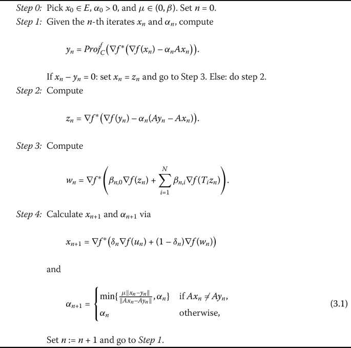
A self-adaptive Tseng extragradient method with Bregman distance (Alg. 3.4)
-
(ii)
In [32, 35, 55, 63], the authors employed a line search technique which uses inner loops and might consume additional computation time for determining the stepsize. In Algorithm 1 we use a self-adaptive method which is very simple and does not possess any inner loop.
-
(iii)
Our work also improves and extends the results of [55, 60–63] on finding a common solution of \(VIP(C,A)\) and a fixed point problem from real Hilbert spaces and 2-uniformly convex Banach spaces to real reflexive Banach spaces.

Remark 3.4
Note that in case where \(x_{n} = y_{n} = w_{n}\), we arrived at a common solution of the VIP and fixed point of \(T_{i}\) (\(i=1,2,\dots ,N\)). In our convergence analysis, we implicitly assumed that this does not occur after finite iterations so that Algorithm 1 generates infinitely many iterations. More so, it is easy to see that the sequence \(\{\alpha _{n}\}\) generated by (3.1) is monotonically nonincreasing and bounded below by \(\min \{ \frac{\mu }{L},\alpha _{0} \} \). Hence, \(\lim_{n\to \infty }\alpha _{n}\) exists.
Lemma 3.5
Let \(\{x_{n}\}\), \(\{y_{n}\}\), \(\{z_{n}\}\) be sequences generated by Algorithm 1 and \(u \in \Gamma \). Then
for all \(n \geq 0\).
Proof
Since \(u \in \Gamma \), then
Note that from (2.5) we have
Thus it follows from (3.2) and (3.3) that
Also from (2.4) we have
Then from (3.4) and (3.5) we obtain
Moreover, by the definition of \(y_{n}\) and using Lemma 2.5 (i), we obtain
Also, since \(u \in VI(C,A)\) and A is pseudo-monotone, it follows that
Combining (3.7) and (3.8), we get
Therefore it follows from (3.6) that
Using the Cauchy–Schwarz inequality and (3.1) with (2.6), we obtain
□
Next, we show that the sequences generated by Algorithm 1 are bounded.
Lemma 3.6
Let \(\{x_{n}\}\) be the sequence generated by Algorithm 1. Then \(\{x_{n}\}\) is bounded.
Proof
Let \(u^{*} \in \Gamma \), from Lemma 3.5 we obtain
Since \(\lim_{n \rightarrow \infty }\alpha _{n}\) exists and \(\mu \in (0,\beta )\), then
This implies that there exists \(N>0\) such that
Hence from (3.10) we get
Also from Lemma 2.9 we obtain
Therefore
Since the sequence \(\{u_{n}\}\) is bounded and ∇f is bounded on bounded subsets of E, there exists a real number \(\rho >0\) such that \(D_{f}(u,u_{n}) \leq \rho \) for all \(n \in \mathbb{N}\). Hence, by induction, we obtain
Thus \(\{D_{f}(u,x_{n})\}\) is bounded, and this implies that \(\{x_{n}\}\) is bounded. Consequently, \(\{y_{n}\}\), \(\{z_{n}\}\), \(\{w_{n}\}\) are bounded too. □
Lemma 3.7
Let \(\{x_{n}\}\) be the sequence generated by Algorithm 1. Then \(\{x_{n}\}\) satisfies the following inequalities:
-
(i)
\(a_{n+1} \leq (1-\delta _{n})a_{n} + \delta _{n} b_{n}\),
-
(ii)
\(-1 \leq b_{n} < +\infty \),
where \(a_{n} = D_{f}(u,x_{n})\), \(b_{n} = \langle \nabla f(u_{n}) - \nabla f(u), x_{n+1} - u \rangle \), and \(u \in \Gamma \) for all \(n \in \mathbb{N}\).
Proof
(i) Let \(u \in \Gamma \), in view of (2.7) and Lemma 2.10, we have
Furthermore, using (2.8), we have
Thus, we established (i).
(ii) Since \(\{x_{n}\}\) and \(\{u_{n}\}\) are bounded, then
This implies that \(\limsup_{n\to \infty }b_{n} < \infty \). Next we show that \(\limsup_{n\to \infty }b_{n} \geq -1\). On the contrary, suppose \(\limsup_{n\to \infty }b_{n} < -1\). Then we can choose \(n_{0} \in \mathbb{N}\) such that \(b_{n} < -1\) for all \(n \geq n_{0}\). Then, for all \(n \geq n_{0}\), we get from (i)
Taking lim sup of the last inequality, we obtain
This contradicts the fact that \(\{a_{n}\}\) is a nonnegative sequence. Hence \(\limsup_{n\to \infty }b_{n} \geq -1\). □
We now prove the convergence of Algorithm 1.
Theorem 3.8
Suppose that \(\{x_{n}\}\) is generated by Algorithm 1. Then \(\{x_{n}\}\) converges strongly to a point x̄, where \(\bar{x} = Proj_{\Gamma }^{f}(\bar{x})\).
Proof
Let \(u \in \Gamma \) and \(a_{n} = D_{f}(u,x_{n})\). We consider the following two possible cases.
Case I: Suppose that \(\{a_{n}\}\) is monotonically decreasing. Since \(\{a_{n}\}\) is bounded, then \(a_{n} - a_{n+1} \to 0\). From (3.11), we have
This implies that
Since \(\delta _{n} \to 0\) as \(n \to \infty \), it follows from (3.12) that
Also, since \(\liminf_{n\to \infty }\beta _{n,0}\beta _{n,i} >0\) and by the property of \(\rho _{r}^{*}\), we obtain
Moreover, f is uniformly Fréchet differentiable, then \(\nabla f^{*}\) is uniformly continuous on bounded subsets of \(E^{*}\), and thus
Furthermore, from Lemma 3.5, we have
This implies that
This implies that
and hence
Since \(\mu \in (0,\beta )\), we get
This implies that
Consequently,
Then
It is clear that
Hence, since \(\nabla f^{*}\) is norm-to-norm continuous on bounded subsets of \(E^{*}\), we obtain
therefore
Since \(\{x_{n}\}\) is bounded, there exists a subsequence \(\{x_{n_{j}}\}\) of \(\{x_{n}\}\) such that \(x_{n_{j}} \rightharpoonup x^{*} \in C\). We now show that \(x^{*} \in \Gamma \). Since \(y_{n_{j}} = Proj_{C}^{f}(\nabla f^{*}(\nabla f(x_{n_{j}}-\alpha _{n_{j}}Ax_{n_{j}})))\), it follows from Lemma 2.5 (i) that
Then
This implies that
Since \(\|x_{n_{j}}- y_{n_{j}}\|\to 0\) and f is strongly coercive, then
Fix \(x \in C\), it follows from (3.15), (3.16) and the fact that \(\liminf_{j\to \infty }\alpha _{n_{j}}>0\), that
Now let \(\{\epsilon _{j}\}\) be a sequence of decreasing nonnegative numbers such that \(\epsilon _{j} \to 0\) as \(j \to \infty \). For each \(\epsilon _{j}\), we denote by \(n_{j}\) the smallest positive integer such that
where the existence of \(n_{j}\) follows from (3.17). Since \(\lbrace \epsilon _{j} \rbrace \) is decreasing, then \(\lbrace n_{j} \rbrace \) is increasing. Also, for each j, \(Ax_{n_{j}} \neq 0\) and, setting
one gets \(\langle Ax_{n_{j}},t_{n_{j}} \rangle =1\) for each k. Therefore,
Since A is pseudo-monotone, we have from (3.17) that
Since \(\lbrace x_{n_{j}} \rbrace \) converges weakly to \(x^{*}\) as \(j \to \infty \) and A is weakly sequentially continuous, we have that \(\lbrace Ax_{n_{j}} \rbrace \) converges weakly to \(Ax^{*}\). Suppose \(Ax^{*} \neq 0\) (otherwise, \(x^{*} \in VI(C,A)\)). Then, by the sequentially weakly lower semicontinuity of the norm, we get
Since \(\lbrace x_{n_{j}} \rbrace \subset \lbrace x_{n_{j}} \rbrace \) and \(\epsilon _{j} \to 0\) as \(j \to \infty \), we get
and this means \(\lim_{j \to \infty } \|\epsilon _{j} t_{2n_{j}}\|=0\). Passing the limit \(j \to \infty \) in (3.18), we get
Therefore, from Lemma 2.13, we have \(x^{*} \in VI(C,A)\). Furthermore, following from (3.13) and (3.14), we have that \(x^{*} \in \hat{F}(T_{i}) = F(T_{i})\) for all \(i =1,2,\dots ,N\), hence \(x^{*} \in \bigcap_{i=1}^{N} F(T_{i})\). Therefore \(x^{*} \in \Gamma \).
We now show that \(\{x_{n}\}\) converges strongly to a point \(\bar{x} = Proj_{\Gamma }^{f}(\bar{x})\). To do this, it suffices to show that \(\limsup_{n\to \infty }\langle \nabla f(u_{n})- \nabla f(\bar{x}), x_{n+1} - \bar{x} \rangle \leq 0\). Choose a sequence \(\{x_{n_{j}}\}\) of \(\{x_{n}\}\) such that
Since \(u_{n_{j}} \to u^{*}\) and \(x_{n_{j}} \rightharpoonup x^{*}\), it follows from Lemma 2.5 (i) that
Hence
Putting \(u = \bar{x}\) in Lemma 3.7, it follows from Lemma 2.14 and (3.19) that \(\lim_{n \rightarrow \infty }a_{n} = 0\). Consequently, \(\lim_{n \rightarrow \infty }\|x_{n} - \bar{x}\| = 0\). This implies that \(\{x_{n}\}\) converges strongly to a point \(\bar{x} = Proj_{\Gamma }^{f}(\bar{x})\).
Case II: Suppose that \(\{a_{n}\}\) is not monotonically decreasing, that is, there is a subsequence \(\{a_{n_{j}}\}\) of \(\{a_{n}\}\) such that \(a_{n_{j}} < a_{n_{j}+1}\) for all \(j \in \mathbb{N}\). Then, by Lemma 2.15, we can define an integer sequence \(\{\tau (n)\}\) for all \(n \geq n_{0}\) by
Moreover, \(\{\tau (n)\}\) is a nondecreasing sequence such that \(\tau (n) \to \infty \) as \(n \to \infty \) and \(a_{\tau (n)}\leq \Gamma _{\tau (n)+1}\) for all \(n \geq n_{0}\). Following a similar argument as in Case I, we obtain
By a similar argument as in Case A, we also obtain
Also, by Lemma 3.7 (i), we get
This implies that
Hence from (3.20) we obtain \(\limsup_{n\rightarrow \infty }D_{f}(u,x_{\tau (n)}) \leq 0\), which implies that \(\lim_{n \rightarrow \infty }D_{f}(u, x_{\tau (n)}) = 0\). Consequently, we have
Hence \(D_{f}(u,x_{n}) \to 0\). This implies that \(\|x_{n} - u\| \to 0\), and thus \(x_{n} \to u = Prof_{\Gamma }^{f}(u)\). This completes the proof. □
The following can be obtained directly as consequences of our main result.
(i) If \(A:E \to E^{*}\) is monotone and Lipschitz continuous on E, then we obtain the following result.
Corollary 3.9
Let E be a real reflexive Banach space, \(A:E \to E^{*}\) be a monotone and Lipschitz continuous operator, and \(\{T_{i}\}\) (\(i =1,2,\dots ,N\)) be a finite family of Bregman quasi-nonexpansive mappings on E such that \(F(T_{i}) = \hat{F}(T_{i})\) for \(i=1,2,\dots ,N\). Let \(f:E \to \mathbb{R}\cup \{+\infty \}\) be a function satisfying Assumption 3.2and \(\{\beta _{n,i}\}\), \(\{\delta _{n}\}\), and \(\{u_{n}\}\) be sequences satisfying Assumption 3.3. Suppose \(\Gamma = VI(C,A) \cap \bigcap_{i=1}^{N} F(T_{i}) \neq \emptyset \). Then the sequence \(\{x_{n}\}\) generated by Algorithm 1 converges strongly to a solution x̄, where \(\bar{x} = Proj_{\Gamma }^{f}(\bar{x})\).
Note that in this case the weak sequential continuity of A in Assumption 3.1 (b) has to be dropped since it follows from the monotonicity and (3.15) that
Passing limit to the above inequality and using the facts that \(\|x_{n_{j}} - y_{n_{j}}\| \to 0\) and \(\|\nabla f(x_{n_{j}}) - \nabla f(y_{n_{j}}) \| \to 0\), we obtain
(ii) In addition, if we take \(\{T_{i}\}\) (\(i=1,2,\dots ,N\)) as a finite family of Bregman nonexpansive mappings on E, then we obtain the following result.
Corollary 3.10
Let E be a real reflexive Banach space and \(A:E \to E^{*}\) and \(f:E \to \mathbb{R}\cup \{+\infty \}\) satisfy Assumptions 3.1and 3.2respectively, where \({T_{i}} \) (\(i=1,2,\dots ,N\)) is a finite family of Bregman nonexpansive mappings. Suppose that \(\{\beta _{n,i}\}\subset (0,1)\) and \(\{\delta _{n}\} \subset (0,1)\) \(\{u_{n}\} \subset E\) satisfy Assumption 3.3. Then the sequence generated by Algorithm 1 converges strongly to a point x̄, where \(\bar{x} = Proj_{\Gamma }(\bar{x})\).
4 Applications
In this section, we give some applications of our result to a generalized Nash equilibrium problem and bandwidth allocation problem.
1. Generalized Nash equilibrium problem (GNEP)
Let \(I=\{1,2,\dots ,N\}\) be the set of players with each player \(i \in I\) controlling variable \(x^{i} \in \mathcal{C}_{i} \subset \mathbb{R}^{m_{i}}\) and \(\mathcal{C} = \prod_{i \in I} \mathcal{C}_{i} \subset \prod_{i \in I} \mathbb{R}^{m_{i}}\), where \(m_{i}\) (\(i\in I\)) satisfy \(m = \sum_{i=1}^{N} m_{i}\). The point \(x^{i}\) is called the strategy of the ith player. We denote by \(x \in \mathbb{R}^{m}\) the vector of strategies \(x = (x_{1},\dots ,x_{N})\), and \(x^{-i}\) denotes the vector formed by all player decision variables \(x^{j}\) except the player i. Thus, we can write \(x = (x^{i}, x^{-i})\), which is the shorthand to denote the vector \(x = (x^{1}, \dots , x^{i-1},x^{i},x^{i+1},\dots ,x^{N} )\). The set \(\mathcal{C}_{i}(x^{-i}) = \{x^{i}\in \mathbb{R}^{m_{i}}: (x^{i},x^{-i}) \in \mathcal{C}\}\) denotes the strategy set of the ith player when the remaining player chooses strategies \(x^{-i}\) (see e.g. [53]). We note that the aim of the ith player given the strategy \(x^{-i}\) is to choose a strategy \(x^{i}\) such that \(x^{i}\) solves the following minimization problem:
For any given \(x^{-i}\), we denote the solution set of (4.1) by \(Sol_{i}(x^{-i})\). Using the above notation, we give the precise definition of the GNEP as follows (see e.g. [32]).
Definition 4.1
A GNEP is defined as finding \(\bar{x} \in \mathcal{C}\) such that \(\bar{x}^{i} \in Sol_{i}(\bar{x}^{-i})\) for every \(i \in I\).
The following result follows from the first order optimality condition for the solution of problem (4.1) for each \(i\in I\).
Theorem 4.2
Consider the GNEP such that
-
(a)
\(\mathcal{C}\) is closed and convex,
-
(b)
\(\theta _{i}\) is continuously differentiable for every \(i \in I\),
-
(c)
\(\theta _{i}(\cdot ,x^{-i}):\mathbb{R}^{m_{i}} \to \mathbb{R}\) is convex for every \(i \in I\) and every \(x \in \mathcal{C}\).
Define an operator \(F:\mathbb{R}^{m} \to \mathbb{R}^{m}\) as
where \(\nabla _{x^{i}}\theta _{i}\) denotes the gradient of \(\theta _{i}\) with respect to its first argument. Then every solution of \(VIP(\mathcal{C},F)\) is a solution of the GNEP.
In addition, the sets \(\mathcal{C}_{i}\) can be defined as the intersection of simpler closed convex sets \(\mathcal{C}_{i}^{(j)}\) (\(j=1,2,\dots ,l_{i}\)) i.e.
Let \(T:\mathbb{R}^{m_{i}} \to \mathbb{R}^{m_{i}}\) be defined by
with the projections \(\Pi _{\mathcal{C}_{i}}^{(j)}: \mathbb{R}^{m_{i}} \to \mathcal{C}_{i}^{(j)} \) (\(i \in I\), \(j = 1,2,\dots ,l_{i}\)) and \(\omega _{i}^{(j)} >0\) (\(i \in I\), \(j=1,2,\dots ,l_{i}\)) such that \(\sum_{j=1}^{l_{i}}\omega _{i}^{(j)}=1\). Then T is nonexpansive (see [2]) and satisfies \(F(T) = \prod_{i\in I}\mathcal{C}_{i} = \mathcal{C}. \nonumber \) Hence, the GNEP can be expressed as the following variational inequality:
It is worthy to mention that formulation (4.3) offers a simple approach of dealing with the GNEP since the sets \(\mathcal{C}_{i}^{(j)}\) can have closed form expressions. This can be applied to more general cases, where the projection onto \(\mathcal{C}\) is not necessarily easy, while the computations of projections \(\Pi _{\mathcal{C}_{i}^{(j)}}\) (\(i\in I\), \(j =1,2,\dots ,l_{i}\)) are in fact traceable.
By choosing \(f(x) = \|x\|^{2}\) and \(N=1\) in Algorithm 1, we can then apply our result to solving the GNEP as follows.
Corollary 4.3
Suppose that the GNEP is consistent (i.e. has a solution), and let \(\mathcal{C}\), F, and T be as defined above such that ∇F is monotone and Lipschitz continuous. Then the sequence \(\{x_{n}\}\) generated by Algorithm 1 converges strongly to a solution of the GNEP.
2. Utility-based bandwidth allocation problem
Efficient network distribution is very important for making communication networks reliable and stable. Network resources such as power, channel, and bandwidth are shared among many sources. In utility-based bandwidth network, the objective is to share available bandwidths among different traffic sources so as to maximize the overall utility under a capacity constraint [46, 58].
The utility based allocation problem can be modeled as a function \(\mathcal{U}\) of the transmission rates allocated to the traffic source which represents the efficiency and fairness of the bandwidth sharing [58]. \(\mathcal{U}\) is typically assumed to be concave and continuously differentiable. A well-known utility function is the weighted proportionally fair function defined by \(\mathcal{U}_{pf}(x) = \sum_{i\in I}\omega _{i} \log (x_{i})\) for all \(x:=(x_{1},x_{2},\dots ,x_{m})^{T} \in \mathbb{R}^{m}_{+}\backslash \{0\}\), where \(x_{i} >0\) denotes the transmission rate of source \(i \in I=\{1,2,\dots ,m\}\), \(\omega _{i} >0\) is the weighted parameter for source i, and \(\mathbb{R}^{m}_{+}:=\{(x_{1},x_{2},\dots ,x_{m})^{T}\in \mathbb{R}^{m}: x_{i} \geq 0, (i \in I)\}\). The optimal bandwidth allocation corresponding to \(\mathcal{U}_{pf}\) is said to be weighted proportionally fair.
The capacity constraint for each line can be expressed as an inequality constraint in which the total sum of the transmission rate for all source sharing the link is less than or equal to the capacity of the link. For each link \(l \in \mathcal{L} = \{1,2,\dots ,L\}\), the capacity constraint is expressed as \(\mathbb{R}_{+}^{m} \cap C_{l}\), where
\(c_{l}>0\) stands for the capacity of link l, and \(I_{i,l}\) takes the value 1 if l is the link used by source s, and 0 otherwise. Then the objective in bandwidth allocation is to solve the following utility-based bandwidth allocation problem [58, Chap. 2] for maximizing the utility function subject to the capacity constraints:
where \(C \subset \mathbb{R}^{m}\) is the capacity constraint set defined by
Note that the set C (4.5) can be expressed as the fixed point set of a mapping composed of the projections onto \(C_{l}s\). Let us define a mapping \(T_{proj}:\mathbb{R}^{m} \to \mathbb{R}^{m}\) composed of the projections onto \(\mathbb{R}^{m}_{+}\) and \(C_{l}s\) as follows:
where \(P_{D}\) stands for the projection onto a nonempty, closed and convex set \(D \subset \mathbb{R}^{m}\). Then \(T_{proj}\) satisfies the nonexpansivity condition because \(P_{\mathbb{R}^{m}_{+}}\) and \(P_{C_{l}}s\) are nonexpansive. Moreover, C coincides with the fixed point set of \(T_{proj}\) [2, Proposition 2.10] i.e.
Also, \(-\nabla \mathcal{U}_{pf}\) is strongly monotone and Lipschitz continuous on a certain set. Then the bandwidth allocation problem (4.4) can be expressed as a common variational inequality and fixed point problem as follows:
Choosing \(f(x) = \|x\|^{2}\) and \(N=1\) in Algorithm 1, we apply Algorithm 1 to solving the utility-based bandwidth network allocation as follows.
Corollary 4.4
Suppose that the utility based allocation problem (4.4) is consistent, and let \(\mathcal{U}_{pf}\), \(T_{proj}\) and the capacity constraint C be defined as above. Then the sequence \(\{x_{n}\}\) generated by Algorithm 1 converges strongly to a solution of Problem (4.4).
5 Numerical experiments
In this section, we present some numerical experiments for our proposed algorithm. We compare the performance of Algorithm 1 for different types of convex functions listed below and with some other algorithms in the literature. All codes are written with a Lenovo PC with the following specification: Intel(R)core i7-5600, CPU 2.48 GHz, RAM 8.0 GB, MATLAB version 9.5 (R2019b).
Example 5.1
Let \(E = \mathbb{R}^{m}\) and \(A: \mathbb{R}^{m} \to \mathbb{R}^{m}\) be defined by \(A(x) = Mx +q\), where
such that B is an \(m \times m\) matrix, S is an \(m \times m\) skew symmetric matrix, D is an \(m \times m\) diagonal matrix whose diagonal is nonnegative (so M is positive definite) and q is a vector in \(\mathbb{R}^{m}\). The feasible set C is defined by \(C = \{x = (x_{1},\dots ,x_{m})^{T}:\|x\| \leq 1 \textit{ and } x_{j} \geq a, j=1,\dots ,m \}\), where \(a <1/\sqrt{m}\). It is clear that A is monotone and Lipschitz continuous with Lipschitz constant \(L = \|M\|\). For \(q =0\), the unique solution of the corresponding VI is \(\{0\}\). We define the mapping \(T_{i}: \mathbb{R}^{m} \to \mathbb{R}^{m}\) as the projection onto C for \(i =1,2,\dots ,5\), which is Bregman nonexpansive (see [51]). The starting point \(x_{0} \in [0,1]^{m}\) and the entries of matrices B, S, D are generated randomly for \(m = 5, 20,50,100\). We choose \(\alpha _{0} = 0.23\), \(\mu = 0.36\), \(\delta _{n} = \frac{1}{n+1}\), \(u_{n} = \frac{1}{n^{5}}\), \(\beta _{n,i} = \frac{1}{6}\) for \(i = 0,1,2,\dots ,5\), and \(n \in \mathbb{N}\). We test Algorithm 1 using \(f^{KL}\), \(f^{SE}\), \(f^{IS}\), \(f^{SM}\) given in Example 2.4
We also compare the performance of Algorithm 1 with Algorithm 3.1 of Thong and Hieu [60] and Algorithm 3.1 of Thong and Hieu [61]. For [60] algorithm, we choose \(\gamma = 2\), \(l = 0.2\), \(\mu = 0.36\), \(\beta _{n} = \frac{2n}{3n+4}\), \(\alpha _{n} = \frac{1}{n+1}\), and \(f(x) = \frac{x}{2}\). We also choose for [61] algorithm \(\mu = 0.36\), \(\tau _{0} = 0.23\), \(\beta _{n} = \frac{n}{5n+5} \quad \forall n \in \mathbb{N}\). The projection onto C is calculated explicitly, and we stop the iterations when \(\|x_{n+1} - x_{n}\| < 10^{-4}\). The computational results are shown in Table 1 and Fig. 1.

Experiment 1, top left: \(m=5\); top right: \(m=20\); bottom left: \(m=50\); bottom right: \(m=100\)
Next, we consider an example in an infinite dimension space where A is a pseudo-monotone and Lipschitz continuous operator but not monotone. In this example, we choose \(f(x) = \|x\|^{2}\) and compare our Algorithm 1 with Algorithm 2 of Thong and Vuong [63].
Example 5.2
Let \(E=L_{2}([0,1])\) endowed with inner product \(\langle x,y \rangle = \int _{0}^{1}x(t)y(t)\,dt\) for all \(x,y \in L_{2}([0,1])\) and norm \(\|x\| = (\int _{0}^{1}|x(t)|^{2}\,dt )^{\frac{1}{2}}\) for all \(x \in L_{2}([0,1])\). Let \(C = \{x \in L_{2}([0,1]):\langle y,x\rangle \leq a\}\), where \(y= 3t^{2}+9\) and \(a =1\). Define \(g:C \rightarrow \mathbb{R}\) by \(g(u) = \frac{1}{1+\|u\|^{2}}\) and \(F: L^{2}([0,1]) \rightarrow L^{2}([0,1])\) as the Volterra integral operator given by \(F(u)(t) = \int _{0}^{t} u (s)\,ds\) for all \(u \in L^{2}([0,1])\) and \(t\in [0,1]\). F is bounded, linear, and monotone with \(L = \frac{\pi }{2}\). Let \(A: L^{2}([0,1])\rightarrow L^{2}([0,1])\) be defined by \(A(u)(t) = (g(u)F(u))(t)\). It is easy to show that A is L-Lipschitz continuous, pseudo-monotone, and not monotone. We choose \(\alpha _{0} = 0.09\), \(\mu = 0.34\), \(T_{i} x = x\), \(N=1\), \(\beta _{m,i} = \frac{n}{2n+2}\), and \(\delta _{n} = \frac{1}{\sqrt{n+1}}\), \(\forall n \in \mathbb{N}\). For Algorithm 2 of [63], we take \(\gamma = 2\), \(l = 0.02\), \(\mu = 0.34\), \(\alpha _{n} = \frac{1}{\sqrt{n+1}}\), \(\beta _{n} = \frac{1 - \alpha _{n}}{2}\), \(\forall n \in N\). We test the algorithms with the following initial points:
-
Case I:
\(x_{0} = \frac{\cos (2t)}{6}\),
-
Case II:
\(x_{0} = \exp (2t) + \sin (3t)\),
-
Case III:
\(x_{0} = \frac{\exp (-3t)}{7}\),
-
Case IV:
\(x_{0} = t^{3} + 2t +3\).
We stop the algorithms when \(\|x_{n+1} -x_{n}\|<10^{-4}\) is reached and plot the graphs of error (\(\|x_{n+1}-x_{n}\|\)) against a number of iterations. The numerical results are shown in Table 2 and Fig. 2.

Experiment 2, top left: Case I; top right: Case II; bottom left: Case III; bottom right: Case IV
Example 5.3
Let \(E = \ell _{3}(\mathbb{R})\), where \(\ell _{3}(\mathbb{R}) = \{x = (x_{1},x_{2},\dots ,x_{i},\dots ), x_{i} \in \mathbb{R}: \sum_{i=1}^{\infty }|x_{i}|^{3} < \infty \}\) with norm \(\|x\|_{\ell } = (\sum_{i=1}^{\infty }|x_{i}|^{3} )^{\frac{1}{3}}\) for \(x \in E\). Let \(C = \{x \in E: \|x\|_{\ell _{3}} \leq 1\}\). For all \(x \in E\), we define the operator \(A:E \to E\) be
Then A satisfies Assumption 3.1 (b). Let \(f:E \to \mathbb{R}\) be defined by \(f(x) = \frac{1}{3}\|x\|_{\ell _{3}}^{3}\) for all \(x \in \ell _{3}(\mathbb{R})\). Also, let \(\{e_{n}\}\) be the standard basis of \(\ell _{3}\) defined by \(e_{n} = (\delta _{n,1},\delta _{n,2},\dots )\) for each \(n \in \mathbb{N}\), where
and \(T:E \to E\) be defined by
Clearly, \(F(T) = \{0\}\) and T is Bregman quasi-nonexpansive (see [59]). We choose the following parameters for our computation: \(\beta _{n} = \frac{1}{100(n+1)} \), \(\delta _{n} = \frac{50n}{70n+3}\), \(\mu =0.26\), \(\alpha _{0} = 0.0025\), \(u_{n} = \frac{x_{0}}{n+1}\). We compare the performance of Algorithm 1 with Algorithm 3.6 of [33] (namely BSEM) and Algorithm 3.3 of [34] using the following initial value:
Case I: \(x_{0} = (1, \frac{1}{\sqrt{2}}, \frac{1}{\sqrt{3}},\dots )\);
Case II: \(x_{0} = (25, 5, 1, \dots )\);
Case III: \(x_{0} = (2, 2, 1,1, \dots )\);
Case IV: \(x_{0} = (1, 0, 1, 0, \dots )\).
We plot the graphs of error (\(\|x_{n+1} - x_{n}\|_{\ell _{3}}\)) against a number of iterations using \(\|x_{n+1} - x_{n}\|_{\ell _{3}} < 10^{-4}\) as the stopping criterion. The computational results are shown in Table 3 and Fig. 3.

Example 5.3, top left: Case I; top right: Case II;bottom left: Case III; bottom right: Case IV
6 Conclusion
This paper introduced a single projection method using Bregman distance techniques for finding a common element in the set of solutions of variational inequalities and the set of common fixed points of a finite family of Bregman quasi-nonexpansive mappings in the framework of a reflexive Banach space. The stepsize of the algorithm is selected self-adaptively, and strong convergence theorem is proved without using the Lipschitz constant of the cost operator as an input parameter. Some applications to generalized Nash equilibrium and bandwidth network problems were given, and some numerical examples were also presented to illustrate the performance of the algorithm. This result improves and extends several results such as [35, 45, 55, 60–63] in the literature.
Availability of data and materials
Not applicable.
References
Alber, Y., Ryazantseva, I.: Nonlinear Ill-Posed Problems of Monotone Type. Springer, Dordrecht (2006)
Bauschke, H.H., Borwein, J.M.: On projection algorithms for solving convex feasibility problems. SIAM Rev. 38, 367–426 (1996)
Bauschke, H.H., Borwein, J.M.: Legendre functions and the method of random Bregman projection. J. Convex Anal. 4, 27–67 (1997)
Bauschke, H.H., Borwein, J.M., Combettes, P.L.: Essential smoothness, essential strict convexity and Legendre functions in Banach space. Commun. Contemp. Math. 3, 615–647 (2001)
Bregman, L.M.: The relaxation method for finding common points of convex sets and its application to the solution of problems in convex programming. USSR Comput. Math. Math. Phys. 7, 200–217 (1967)
Butnariu, D., Iusem, A.N.: Totally Convex Functions for Fixed Points Computational and Infinite Dimensional Optimization. Kluwer Academic, Dordrecht (2000)
Butnariu, D., Resmerita, E.: Bregman distances, totally convex functions and a method for solving operator equations in Banach spaces. Abstr. Appl. Anal. 2006, Article ID: 84919, 1–39 (2006)
Cai, G., Gibali, A., Iyiola, O.S., Shehu, Y.: A new double-projection method for solving variational inequalities in Banach spaces. J. Optim. Theory Appl. 178, 219–239 (2018)
Ceng, L.C., Petrusel, A., Qin, X., Yao, J.C.: A modified inertial subgradient extragradient method for solving pseudomonotone variational inequalities and common fixed point problems. Fixed Point Theory 21, 93–108 (2020)
Ceng, L.C., Petrusel, A., Wen, C.F., Yao, J.C.: Inertial-like subgradient extragradient methods for variational inequalities and fixed points of asymptotically nonexpansive and strictly pseudocontractive mappings. Mathematics 7(9), Article ID 860 (2019)
Ceng, L.C., Qin, X., Shehu, Y., Yao, J.C.: Mildly inertial subgradient extragradient method for variational inequalities involving an asymptotically nonexpansive and finitely many nonexpansive mappings. Mathematics 7(10), Article ID 881 (2019)
Ceng, L.C., Shang, M.J.: Hybrid inertial subgradient extragradient methods for variational inequalities and fixed point problems involving asymptotically nonexpansive mappings. Optimization (2019). https://doi.org/10.1080/02331934.2019.1647203
Ceng, L.C., Teboulle, M., Yao, J.C.: Weak convergence of an iterative method for pseudomonotone variational inequalities and fixed-point problems. J. Optim. Theory Appl. 146, 19–31 (2010)
Ceng, L.C., Yuan, Q.: Composite inertial subgradient extragradient methods for variational inequalities and fixed point problems. J. Inequal. Appl. 2019, Article ID 274 (2019)
Censor, Y., Gibali, A., Reich, S.: The subgradient extragradient method for solving variational inequalities in Hilbert spaces. J. Optim. Theory Appl. 148, 318–335 (2011)
Censor, Y., Gibali, A., Reich, S.: Strong convergence of subgradient extragradient methods for the variational inequality problem in Hilbert space. Optim. Methods Softw. 26, 827–845 (2011)
Censor, Y., Gibali, A., Reich, S.: Extensions of Korpelevich’s extragradient method for variational inequality problems in Euclidean space. Optimization 61, 1119–1132 (2012)
Censor, Y., Lent, A.: An iterative row-action method for interval complex programming. J. Optim. Theory Appl. 34, 321–353 (1981)
Chambolle, A.: An algorithm for total variation minimization and applications. J. Math. Imaging Vis. 20(1), 89–97 (2004)
Chidume, C.E., Nnakwe, M.O.: Convergence theorems of subgradient extragradient algorithm for solving variational inequalities and a convex feasibility problem. Fixed Point Theory Algorithms Sci. Eng. 2018, 16 (2018)
Combettes, P.L., Pesquet, J.-C.: Proximal splitting methods in signal processing. In: Fixed-Point Algorithms for Inverse Problems in Science and Engineering, pp. 185–212 (2011)
Denisov, S.V., Semenov, V.V., Chabak, L.M.: Convergence of the modified extragradient method for variational inequalities with non-Lipschitz operators. Cybern. Syst. Anal. 51, 757–765 (2015)
Dong, Q.L., Lu, Y.Y., Yang, J.: The extragradient algorithm with inertial effects for solving the variational inequality. Optimization 65(12), 2217–2226 (2016)
Gibali, A.: A new Bregman projection method for solving variational inequalities in Hilbert spaces. Pure Appl. Funct. Anal. 3(3), 403–415 (2018)
Goldstein, A.A.: Convex programming in Hilbert space. Bull. Am. Math. Soc. 70, 709–710 (1964)
Hai, T.N.: On gradient projection methods for strongly pseudomonotone variational inequalities without Lipschitz continuity. Optim. Lett. 14, 1177–1191 (2020)
He, B.S.: A class of projection and contraction methods for monotone variational inequalities. Appl. Math. Optim. 35, 69–76 (1997)
Hieu, D.V., Cholamjiak, P.: Modified extragradient method with Bregman distance for variational inequalities. Appl. Anal. (2020). https://doi.org/10.1080/00036811.2020.1757078
Hieu, D.V., Thong, D.V.: New extragradient-like algorithms for strongly pseudomonotone variational inequalities. J. Glob. Optim. (2018). https://doi.org/10.1007/s10898-017-0564-3
Iiduka, H.: A new iterative algorithm for the variational inequality problem over the fixed point set of a firmly nonexpansive mapping. Optimization 59, 873–885 (2010)
Iiduka, H., Yamada, I.: A use of conjugate gradient direction for the convex optimization problem over the fixed point set of a nonexpansive mapping. SIAM J. Optim. 19, 1881–1893 (2009)
Iusem, A., Nasri, M.: Korpelevich’s method for variational inequality problem in Banach spaces. J. Glob. Optim. 50, 59–76 (2011)
Jolaoso, L.O., Aphane, M.: Weak and strong convergence Bregman extragradient schemes for solving pseudo-monotone and non-Lipschitz variational inequalities. J. Inequal. Appl. 2020, 195 (2020)
Jolaoso, L.O., Shehu, Y.: Single Bregman projection method for solving variational inequalities in reflexive Banach spaces. Appl. Anal. (2021). https://doi.org/10.1080/00036811.2020.1869947
Jolaoso, L.O., Taiwo, A., Alakoya, T.O., Mewomo, O.T.: A strong convergence theorem for solving pseudo-monotone variational inequalities using projection methods in a reflexive Banach space. J. Optim. Theory Appl. 185(3), 744–766 (2020)
Jolaoso, L.O., Taiwo, A., Alakoya, T.O., Mewomo, O.T.: A unified algorithm for solving variational inequality and fixed point problems with application to the split equality problem. Comput. Appl. Math. 39, 38 (2020). https://doi.org/10.1007/s40314-019-1014-2
Kanzow, C., Shehu, Y.: Strong convergence of a double projection-type method for monotone variational inequalities in Hilbert spaces. J. Fixed Point Theory Appl. 20, 51 (2018). https://doi.org/10.1007/s11784-018-0531-8
Kassay, G., Reich, S., Sabach, S.: Iterative methods for solving system of variational inequalities in reflexive Banach spaces. SIAM J. Optim. 21(4), 1319–1344 (2011)
Konnov, I.V.: Combined Relaxation Methods for Variational Inequalities. Springer, Berlin (2001)
Korpelevich, G.M.: The extragradient method for finding saddle points and other problems. Èkon. Mat. Metody 12, 747–756 (1976) (In Russian)
Kraikaew, R., Saejung, S.: Strong convergence of the Halpern subgradient extragradient method for solving variational inequalities in Hilbert spaces. J. Optim. Theory Appl. 163, 399–412 (2014)
Lin, L.J., Yang, M.F., Ansari, Q.H., Kassay, G.: Existence results for Stampacchia and Minty type implicit variational inequalities with multivalued maps. Nonlinear Anal., Theory Methods Appl. 61, 1–19 (2005)
Maingé, P.E.: Strong convergence of projected subgradient methods for nonsmooth and nonstrictly convex minimization. Set-Valued Anal. 16, 899–912 (2008)
Maingé, P.E.: Projected subgradient techniques and viscosity methods for optimization with variational inequality constraints. Eur. J. Oper. Res. 205, 501–506 (2010)
Mashreghi, J., Nasri, M.: Forcing strong convergence of Korpelevich’s method in Banach spaces with its applications in game theory. Nonlinear Anal. 72, 2086–2099 (2010)
Mo, J., Walrand, J.: Fair end-to-end window-based congestion control. IEEE/ACM Trans. Netw. 8, 556–567 (2000)
Naraghirad, E., Yao, J.-C.: Bregman weak relatively nonexpansive mappings in Banach spaces. Fixed Point Theory Appl. 2013, Article ID 141 (2013)
Phelps, R.R.: Convex Functions, Monotone Operators and Differentiablity, 2nd edn. Lecture Notes in Mathematics, vol. 1364. Spinger, Berlin (1993)
Reem, D., Reich, S., De Pierro, A.R.: Re-examination of Bregman functions and new properties of their divergences. Optimization 68(1), 279–348 (2019)
Reich, S., Sabach, S.: A strong convergence theorem for proximal-type algorithm in reflexive Banach spaces. J. Nonlinear Convex Anal. 10, 471–485 (2009)
Reich, S., Sabach, S.: Two strong convergence theorems for Bregman strongly nonexpansive operators in reflexive Banach spaces. Nonlinear Anal. 73(1), 122–135 (2010)
Reich, S., Sabach, S.: Two strong convergence theorem for a proximal method in reflexive Banach spaces. Numer. Funct. Anal. Optim. 31(13), 22–44 (2010)
Rosen, J.B.: Existence and uniqueness of equilibrium points for concave n-person games. Econometrica 33, 520–534 (1965)
Senakka, P., Cholamjiak, P.: Approximation method for solving fixed point problem of Bregman strongly nonexpansive mappings in reflexive Banach spaces. Ric. Mat. 65(1), 209–220 (2016)
Shehu, Y.: Single projection algorithm for variational inequalities in Banach spaces with applications to contact problems. Acta Math. Sci. 40B(4), 1045–1063 (2020)
Shehu, Y., Dong, Q.L., Jiang, D.: Single projection method for pseudo-monotone variational inequality in Hilbert spaces. Optimization 68, 385–409 (2019)
Solodov, M.V., Svaiter, B.F.: A new projection method for variational inequality problems. SIAM J. Control Optim. 37, 765–776 (1999)
Srikant, R.: Mathematics of Internet Congestion Control. Birkhäuser, Basel (2004)
Taiwo, A., Jolaoso, L.O., Mewomo, O.T.: Inertial-type algorithm for solving split common fixed point problems in Banach spaces. J. Sci. Comput. 86, 12 (2021)
Thong, D.V., Hieu, D.V.: New extragradient methods for solving variational inequality problems and fixed point problems. J. Fixed Point Theory Appl. 20(3), 129 (2018). https://doi.org/10.1007/s11784-018-0610-x
Thong, D.V., Hieu, D.V.: Mann-type algorithms for variational inequality problems and fixed point problems. Optimization (2019). https://doi.org/10.1080/02331934.2019.1692207
Thong, D.V., Vinh, N.T., Cho, Y.J.: A strong convergence theorem for Tseng’s extragradient method for solving variational inequality problems. Optim. Lett. 14, 1157–1175 (2019)
Thong, D.V., Vuong, P.T.: Modified Tseng’s extragradient methods for solving pseudo-monotone variational inequalities. Optimization 68(11), 2207–2226 (2019)
Tseng, P.: A modified forward-backward splitting method for maximal monotone mappings. SIAM J. Control Optim. 38, 431–446 (2009)
Wega, G.B., Zegeye, H.: Convergence results of forward-backward method for a zero of the sum of maximally monotone mappings in Banach spaces. Comput. Appl. Math. 39, 223 (2020)
Xu, H.K.: Iterative algorithms for nonlinear operators. J. Lond. Math. Soc. 66, 240–256 (2002)
Zhao, X., Yao, Y.: Modified extragradient algorithms for solving monotone variational inequalities and fixed point problems. Optimization (2020). https://doi.org/10.1080/02331934.2019.1711087
Acknowledgements
The first author acknowledge, with gratitude, the Department of Mathematics and Applied Mathematics at the Sefako Makgatho Health Sciences University for making their facilities available for the research.
Funding
This first author is supported by the mathematics research grant from the Sefako Makgatho Health Sciences University, South Africa.
Author information
Authors and Affiliations
Contributions
The authors contributed equally to the writing of this paper. All authors approved the final version of the manuscript.
Corresponding author
Ethics declarations
Competing interests
The authors declare that they have no competing interests.
Rights and permissions
Open Access This article is licensed under a Creative Commons Attribution 4.0 International License, which permits use, sharing, adaptation, distribution and reproduction in any medium or format, as long as you give appropriate credit to the original author(s) and the source, provide a link to the Creative Commons licence, and indicate if changes were made. The images or other third party material in this article are included in the article’s Creative Commons licence, unless indicated otherwise in a credit line to the material. If material is not included in the article’s Creative Commons licence and your intended use is not permitted by statutory regulation or exceeds the permitted use, you will need to obtain permission directly from the copyright holder. To view a copy of this licence, visit http://creativecommons.org/licenses/by/4.0/.
About this article

Cite this article
Jolaoso, L.O., Shehu, Y. & Cho, Y.J. Convergence analysis for variational inequalities and fixed point problems in reflexive Banach spaces. J Inequal Appl 2021, 44 (2021). https://doi.org/10.1186/s13660-021-02570-6
Received:
Accepted:
Published:
DOI: https://doi.org/10.1186/s13660-021-02570-6