
Abstract
In this paper we illustrate the simplifications produced by FDR in NNLO computations. We show with an explicit example that—due to its four-dimensionality—FDR does not require an order-by-order renormalization and that, unlike the one-loop case, FDR and dimensional regularization generate intermediate two-loop results which are no longer linked by a simple subtraction of the ultraviolet (UV) poles in \(\epsilon \). Our case study is the two-loop amplitude for \(H \rightarrow \gamma \gamma \), mediated by an infinitely heavy top loop, in the presence of gluonic corrections. We use this to elucidate how gauge invariance is preserved with no need of introducing counterterms in the Lagrangian. In addition, we discuss a possible four-dimensional approach to the infrared problem compatible with the FDR treatment of the UV infinities.
1 Introduction
Computing radiative corrections has become of uppermost importance in particle phenomenology [1]. The present lack of unexpected signals at the LHC pulls the effects of New Physics in a domain where small discrepancies have to be searched via detailed comparisons between experimental results and precise calculations of the Standard Model background. Due to the large QCD coupling constant, precise predictions at the LHC often require NNLO accuracy. On the other hand, calculations based on two or more loops in the complete Electroweak (EW) model will be mandatory at the future International Linear Collider to meet the experimental accuracy foreseen, for example, in Higgs Physics [2].
While NLO techniques are very well established [3–8], [9–15], work is ongoing to solve the NNLO problem in its full generality [16]. As for the virtual sector, progress has been recently achieved by extending generalized unitarity techniques at two loops [17–21], while the antenna subtraction [22, 23] and sector decomposition [24–27] methods look promising tools to deal with IR divergences beyond NLO [28].
In this paper we investigate the possibility of further simplifying NNLO computations by abandoning dimensional regularization [29]. Despite its known virtues, DR requires a heavy analytic work aimed at subtracting powers of \(1/\epsilon \) of UV or IR origin even before attacking the calculation of the finite physical part. For instance, DR forces an order-by-order iterative renormalization, which is especially cumbersome when computing loop corrections in the EW model or in SUSY: the full set of one-loop counterterms has to be determined and added in a two-loop computation, and so on. Furthermore, loop functions used at a given perturbative level must be further expanded in \(\epsilon \)—when appearing at higher orders—to include terms generating \({\mathcal {O}}(\epsilon ^0)\) contributions when multiplied by the new poles. Such complications arise in DR because constants needed to preserve the symmetries of the Lagrangian are often produced by \(\epsilon \epsilon \) terms, which are kept under control by the iterative renormalization.
This has driven us to study the performances of FDR [30] as a simpler four-dimensional approach beyond one loop.Footnote 1 The key point of FDR is that the use of counterterms is avoided by defining a four-dimensional and UV-free loop integration in a way compatible with shift and gauge invariance. Having done this, the correct results automatically emerge once the theory is fixed in terms of physical observables by means of a finite renormalization relating the parameters of the Lagrangian to measured quantities. In addition, IR infinities can be naturally accommodated within the same four-dimensional framework used to cope with the UV divergences. This is why we envisage in FDR a great potential to reduce the complexity of the NNLO calculations, especially when used together with numerical techniques.
In this paper we present, as the first example of a two-loop FDR calculation, the QCD corrections to the top-loop-mediated Higgs decay into two photons, in the limit \(m_\mathrm{top} \rightarrow \infty \). This computation gives the opportunity to fully appreciate the simplifications due to the four-dimensionality of the approach in a realistic two-loop case study.Footnote 2 In the next section we review the general FDR idea with special emphasis on the two-loop case. We discuss, in particular, the shift and gauge invariance properties of the FDR integration, the main differences with DR, and the IR problem. The two-loop FDR calculation of \(H \rightarrow \gamma \gamma \) is presented in Sect. 3 and the technical details are collected in the final appendices.
2 FDR and the importance of working in four dimensions
2.1 Definition of the FDR loop integral
FDR subtracts UV divergences at the integrand level. This is obtained in two steps. Firstly, the propagators of the particles flowing in the loops are given a common additional term \(-\mu ^2\), formally identified with the \(+ i 0\) propagator prescription. For example, vector-boson and fermion propagators with momentum \((q+p_i)\) and mass \(M_i\) read,Footnote 3 in the unitary gauge,

respectively, with
Secondly, UV infinities are isolated by a repeated use of the identity
In fact—being \(d_i\) is at most linear in \(q\)—the second term in the r.h.s. of Eq. (3) is less UV divergent than the original denominator, so that UV divergences can be systematically moved to terms such as \({1}/{\bar{q}^2}\), which depend only on \(\mu \), and directly subtracted from the integrand. Schematically, dubbing \(J\) the original integrand of an \(\ell \)-loop function, one has
where \(J_\mathrm{INF}\) collects the UV divergent integrands. Then the FDR integral over \(J\) is defined asFootnote 4
where, due to the limit \({\mu \rightarrow 0}\), only a logarithmic dependence on \(\mu \) remains, which can be traded for a dependence on the renormalization scale.Footnote 5 Thus, FDR and normal integration coincide in a convergent integral, since no divergent part \(J_\mathrm{INF}\) can be extracted from its integrand. Furthermore, the space-time is kept strictly four-dimensional also in divergent integrals—with \(g^{\alpha \beta }= \mathrm{diag}(1,-1,-1,-1)\)—because \(\mu ^2\) is nothing but the infinitesimal deformation needed to define the loop integralsFootnote 6 and it is not generated by higher-dimensional components of the integration momenta. This allows one to perform, in particular, the Dirac gamma algebra in four dimensions, with extra rules needed to keep gauge invariance, as explained in Sect. 2.4.
An explicit example of integrand FDR expansionFootnote 7 at one loop is given by
where \(p_0= 0\) and the terms in square brackets are proportional to UV divergent integrands. A two-loop example with
reads
where
Note that identities such as
are needed to extract the sub-divergences. Then the one- and two-loop FDR integrals over the integrands in Eqs. (6) and (8) read
It is important to realize that divergent tensor structures are fully subtracted from the original integrand, as in Eq. (6).Footnote 8 Owing to the Lorentz invariance and four-dimensionality of this definition, irreducible tensors can be decomposed in terms of scalars. For exampleFootnote 9
can be rewritten as
with
Finally, polynomials in the integration variables represent a limiting case of Eq. (4), in which
As a consequence
for any integer \(\alpha \ge 0\).
2.2 Shift invariance and uniqueness
FDR integrals are invariant under the shift of any integration variable. This can easily be proven by using the fact that they can be thought of as finite differences of shift-invariant dimensionally regulatedFootnote 10 divergent integrals [see Eq. (4)]
The explicit demonstration is given in Appendix A. A corollary to this theorem is the uniqueness of the definition in Eq. (5). In fact, the subtracted integrands in \(J_\mathrm{INF}(q_1,\ldots , q_\ell )\) are unambiguously determined by the UV content of the original integrand, the only possible ambiguity being shifts of the loop momenta in \(J(q_1,\ldots , q_\ell )\), which, however, produce the same FDR integral.
Equation (17) also demonstrates that whenever DR loop integrals are known, their FDR counterparts can also be computed.
2.3 Independence of the cutoff
As a result of the subtraction of the divergent integrands, non integrable powers of \(1/\bar{q}^2\) are developed in \(J_{\mathrm{F},\ell }(q_1,\ldots , q_\ell )\). Such IR poles get regulated by the \(\mu ^2\) propagator prescription, which gives a meaning to the r.h.s. of Eq. (5). Thus, the original UV cutoff is traded for an IR one: \(\mu \). Here we show that FDR integrals depend at most logarithmically on \(\mu \). Furthermore, \(\mu \) can be traded for the renormalization scale \(\mu _\mathrm{R}\), rendering the definition of the FDR integration independent of any cutoff.
We start from Eq. (17). Since the first term in its r.h.s. is the original DR regulated integral it does not depend on \(\mu \), in the limit \(\mu \rightarrow 0\).Footnote 11 On the other hand, polynomially divergent integrands in \(J_\mathrm{INF}\) cannot contribute either, because they generate polynomials in \(\mu \). Therefore, the \(\mu \) dependence in the l.h.s. is entirely due to powers of \(\ln (\mu /\mu _\mathrm{R})\) created by the subtraction of the logarithmically divergent integrals. If one redefines FDR integrals without subtracting such logarithms, no dependence on \(\mu \) is produced. This is equivalent to the operation of adding back all \(\ln (\mu /\mu _\mathrm{R})\)s to the l.h.s. of Eq. (17). Then the limit \({\mu \rightarrow 0}\) can be taken, \(\mu \) becomes \(\mu _\mathrm{R}\), and no cutoff is left. The identification \(\mu = \mu _\mathrm{R}\) after \(\lim _{\mu \rightarrow 0}\) is understood in all FDR integrals appearing in this paper.
2.4 Keeping gauge invariance
Now we discuss how gauge invariance is preserved in FDR. Our starting point is the existence of graphical proofs of the Ward–Slavnov–Taylor identities [40], in which the correct relations among Green’s functions are demonstrated—at any loop order—directly at the level of Feynman diagrams. Such proofs are valid under two circumstances:
-
divergent loop integrals should be defined in a way that shifting the integration momenta is possible as if they were convergent ones [41];
-
cancelations between numerators and denominators should be preserved.Footnote 12
Since the first property has been already proven, we concentrate here on the second requirement, which we study by means of a two-loop example.
Consider the scalar integral
To define it in FDR, it is necessary to make explicit the \(\mu ^2\) dependence in its denominators,Footnote 13 which amounts to the replacement
However, this change should be performed without altering the cancelations which ensure that the same result is obtained both by simplifying the reducible numerators before computing the integrals and by working out the integrals without simplifying the numerators.
That happens only if
-
1.
any \(q^2_i\) generated by Feynman rules in the numerator of a diagramFootnote 14 is also changed as in Eq. (19);
-
2.
simplifications at the integrand level are possible, such as
$$\begin{aligned}&\!\!\!\int [d^4q_1] [d^4q_2] \frac{q^2_1 -m^2_1-\mu ^2}{\bar{D}_1^3\bar{D}_2\bar{D}_{12}}\nonumber \\&\quad =\int [d^4q_1] [d^4q_2] \frac{1}{\bar{D}_1^2\bar{D}_2\bar{D}_{12}}. \end{aligned}$$(20)
Either way, integrals with \(\mu \) in the numerator appear—which we dub extra integrals—that need to be properly defined. For instance, since an explicit computation gives
one deduces thatFootnote 15
In fact, a non-zero contribution must be added to the l.h.s. of Eq. (21) to produce the r.h.s. of Eq. (20). The right cancelation occurs if the denominators \(1/{\bar{D}_1^3\bar{D}_2\bar{D}_{12}}\) are expanded in front of \(\mu ^2\) as if it was a \(q^2_1\), namely as in Eq. (12)Footnote 16:
By using this definition, Eq. (20) directly follows from the FDR defining expansion of its two sides. Note that the index \(_1\) in \(\mu ^2|_1\) only denotes the expansion to be used: although only one kind of \(\mu ^2\) exists
are in general different, because they are defined by expanding
respectively.
The described procedure is completely general: the extra integrals are defined by the FDR expansion of the integrals obtained by replacing \(\mu |_i \rightarrow q_i\). As a consequence, the \(\mu |_i\) in the numerator are sensitive to changes of variables. For example, if \(q_1 \rightarrow q_1 -q_2\) and \(q_2 \rightarrow -q_2\),
Extra integrals can be computed either directly, by considering the finite part \(J_D(q_1,q_2)\) of the relevant denominator expansion—as done in Eq. (23)—or indirectly, by rewriting \(J_D(q_1,q_2)\) as a difference between the original integrand and its subtracted pieces. This second way is usually more convenient, because the original integral does not contribute in the limit \(\mu \rightarrow 0\). For example, Eq. (125) gives
which coincides with the result in footnote 16.
Finally, extra integrals give the possibility to rewrite tensors in terms of scalars plus constants. For instance, Eq. (13) produces
Decompositions like this will be extensively used in the calculation presented in Sect. 3.
Having studied the general mechanism of the gauge cancelations in FDR, we further elucidate it by means of the process investigated in this paper, namely \(H \rightarrow \gamma \gamma \) mediated by a fermion with mass \(m\). In this case the proof of gauge invariance relies on the graphical equivalence depicted in Fig. 1, which, in turn, is realized by the Feynman identity

where
Consider now the generic \(\ell \)-loop amplitude in Fig. 2.

Graphical representation of the Feynman identity in Eq. (29). The dashed line represents a scalar photon

Generic \(\ell \)-loop amplitude with an external photon with momentum \(p\). The blob stands for the rest of the amplitude and \(q\) is an integration momentum.
Its integrand reads

where the sum is over all contributing Feynman diagrams, and \(\Gamma ^{i}_o\) (\(\Gamma ^{i}_e\)) is proportional to a product of an odd (even) number of gamma matrices. Gauge invariance requires that
where \(\bar{J}^\alpha \) is the integrand in Eq. (31) regulated à la FDR by replacing \(q^2_i \rightarrow q^2_i-\mu ^2\) in both numerators and denominators. Equation (32) can be directly proven at the integrand level. With this aim, we first concentrate on the replacements responsible for the conservation of the specific current in Fig. 2:

where the loop denominators in \(\Gamma ^{i}_{o,e}\) are also barred. In the previous equation

has the effect of changing \(q^2\) to \(\bar{q}^2\) in the first trace. Thus, when contracting with \(p\), it is possible to reconstruct and cancel denominators

in agreement with the Feynman identity in Eq. (29). After that
directly follows from the shift invariance properties of the loop integrals, as in DR. We explicitly tested Eq. (36) up to two loops in \(H \rightarrow \gamma \gamma \).
With more photons, replacements as in Eq. (34) have to be performed for all integration momenta appearing in the trace.Footnote 17 The one-loop prescription is that defined in [38]: given a fermionic string, one chooses arbitrarily the sign of \(\mu \) within the first  ; the sign of the subsequent one is opposite, if an even number of \(\gamma \)-matrices occur between the two
  s, and it is the same otherwise.Footnote 18 This rule is sufficient in the presence of one fermion line only, as in the calculation at hand. With two or more lines, and no summation indices among them, each fermion string can be separately treated as described. If sums occur, after applying the above algorithm, extra \(\mu ^2\) terms need to be extracted according to the following procedure:

where \(\Gamma ^{(k)}\) represents a string of \(k\) gamma matrices. Equation (37) is proven by noting that \(n\) (m) anticommutations are needed to bring  close to \(\gamma _\alpha \) (\(\gamma ^\alpha \)) and can easily be checked by taking the traces and substituting \(q^2 \rightarrow q^2 -\mu ^2\). As an example of such rules, the integrand of the one-loop \(H \rightarrow \gamma (p_1) \gamma (-p_2) \) amplitude is proportional to

and its FDR regulated version reads

which satisfies the Ward identities
We emphasize that there is nothing mysterious in Eq. (39): the same result is obtained by computing the trace in Eq. (38) and replacing \(q^2 \rightarrow \bar{q}^2\). The advantage of Eq. (39) is that it permits a trivial proof of the Ward identities at the integrand level.
The corresponding procedure at two loops is better explained with an example. Consider the trace

which contributes to the second diagram of Fig. 5. Its FDR counterpart reads

with
Equation (42) is obtained from Eq. (41) by using—one after the other—the one-loop replacements  and
and  , which generate the terms proportional to \(\mu ^2|_{1}\) and \(\mu ^2|_{2}\). The \(\tilde{\mu }^2_{12}\) contribution originates, instead, from the substitution
and is obtained by simultaneously barring  and
and  in Eq. (41) (with the same rule used at one loop to determine the sign of \(\mu |_{i}\) inside each
  , without distinguishing between
  and
and  ) and subtracting the \(\mu ^2|_i\) terms already calculated. What is left is, by construction, proportional to powers of \(\mu |_{1}\mu |_{2} \equiv \tilde{\mu }^2_{12}\) and gives the last term in Eq. (42). Once again, \(\bar{T}^{\alpha \beta }\) is equivalent to the replacements
in the original trace \(T^{\alpha \beta }\). Thus, the \(\mu ^2|_{i}\) ensure the right cancelations leading to the fulfillment of the Ward identities. We explicitly checked that the two-loop \(H \rightarrow \gamma (p_1) \gamma (-p_2)\) integrand \(\bar{J}^{\alpha \beta } (q_1,q_2)\), constructed as described, satisfies
In practical cases it is often convenient to simplify reducible numerators before computing the loop integrals. In that way, only irreducible tensors appear and extra integrals are just produced by tensor decomposition, as in Eq. (28). This is the strategy of the calculation presented in Sect. 3.
2.5 FDR versus DR
The proof that DR preserves gauge invariance and unitarity relies on the possibility of introducing order-by-order local counterterms in the Lagrangian \(\mathcal{L}\). On the contrary, FDR makes no reference to \(\mathcal{L}\). In this subsection we use the simple two-loop QED example of [43] to comment on the conceptual differences between the two approaches.
Consider a DR calculation of the one-loop photon self-energy

with
Then, at two loops and up to terms \(\mathcal{O}(\epsilon )\),

Simply removing the poles from the last expression gives \(\Pi _0^2 + 2\Pi _{-1}\Pi _1\), which is not the right result because it violates unitarity. As is well known, the correct procedure to undertake in DR is to renormalize order by order, i.e. to add one-loop counterterms in \(\mathcal{L}\) such that

Thus

In FDR, the divergences are subtracted at the level of the definition of the loop integration, so that the product of two one-loop diagrams is simply the product of the two finite parts, with no need of introducing extra interactions in \(\mathcal{L}\). Thus, one directly obtains

with \(\Pi _\mathrm{FDR}(p^2)= \Pi _0\). This difference can also be understood from the DR \(\leftrightarrow \) FDR naive correspondence
which gives \(\lim _{\epsilon \rightarrow 0} \epsilon /\epsilon = 1\), while \(\lim _{\mu \rightarrow 0} \mu \ln \mu = 0\).
From all that it is manifest that spurious \(\epsilon /\epsilon \) terms such as \(\Pi _{-1}\Pi _1\)—which need to be kept under control in DR by the order-by-order renormalization—never appear in FDR. The result of an FDR calculation typically depends on the parameters contained in \(\mathcal{L}\), and a (finite) global renormalization is needed only to link them to experimental measurements at the desired perturbative accuracy. In particular —and in contrast with DR—no renormalization is necessary when no parameter appears in the final result. This is the case of the calculation presented in Sect. 3.
2.6 FDR versus FDH
In this subsection we discuss the differences between FDR and the Four-Dimensional Helicity scheme (FDH) of [44], which is equivalent to dimensional reduction [45] at one loop. FDH is a variant of DR, in which gauge cancelations are kept by integrating all momentum integrals over \(n\)-component momenta and considering any \(g^{\alpha \beta }\) resulting from the integration as \(n\)-dimensional. Observed external states are treated in four dimensions (preserving supersymmetry) and unobserved internal ones are defined in such a way that the contraction \(q^{\alpha } q^{\beta } g_{\alpha \beta }= q^2\) gives rise to an \(n\)-dimensional object when \(q\) is an integration momentum. If \(q^2\) is split into four-dimensional (\(q^2_4\)) and \(\epsilon \)-dimensional (\(\tilde{q}^2\)) components,
and \(\tilde{q}^2\) is identified with \(-\mu ^2\), there is a formal equivalence—at the integrand level—between the procedures used by FDR and FDH to determine the \(\mu ^2\) pieces [46, 47]. However, differences start when integrating. FDR integration is defined in a way that non-local sub-divergences are subtracted right away, as in the second line of Eq. (8), while in FDH sub-divergences are compensated by counterterms added at a previous renormalization stage, as in any conventional subtraction scheme. It is exactly this peculiarity that makes it possible to avoid an order-by-order renormalization in FDR.
As a consequence of this dissimilarity, integrals containing \(\mu ^2\) give different results, at two loops and beyond, when computed in FDR and FDH. For example
with \(f\) defined in Eq. (130), while
Only at one loop, because no sub-divergences are present, FDR and FDH coincide, as observed in [37]. For instance,
2.7 Infrared divergences
Although the process \(H \rightarrow \gamma \gamma \) is free of IR infinities, we devote this subsection to an illustration of how soft and collinear singularities can be treated compatibly with FDR. We first discuss divergences in the virtual contribution, and then show how they are matched by a particular treatment of the real radiation.
As for the loop integration, the definition in Eq. (5) can be maintained also in the presence of IR singularities. For instance, the FDR versions of the massless one- and two-loop scalar integrals in Fig. 3 read
respectively, withFootnote 19
Note that the on-shell conditions \(p^2_1= p^2_2= 0\) are used at the integrand level. Thus, infrared virtual divergences get regulated by the \(\mu ^2\)-deformed propagators,Footnote 20 which generates powers of logarithms of \(\mu ^2\), upon integration. A particularly interesting situation is when the integral is also UV divergent. In this case it is easy to see that UV divergent scale-less \(\ell \)-loop FDR integrals vanish, as in DR. In fact, the only allowed external variable is a momentum \(p\) such that \(p^2=0\), whose fate is to appear in the numerator of \(J_{\mathrm{F},\ell }(q_1,\ldots , q_\ell )\) in Eq. (4) to improve the UV convergence of the original integrand. Therefore, \(J_{\mathrm{F},\ell }(q_1,\ldots , q_\ell )\) is entirely made of integrands proportional to positive powers of \((q_i \cdot p)\), which vanish, by Lorentz invariance, after integration. The simplest case is the fully massless one-loop 2-point scalar function
The FDR expansion of its integrand reads
so that
The same result is obtained by a direct computation
from which it is manifest that, in the limit \(p^2 \rightarrow 0\), a cancelation occurs between two logarithms of UV and IR origin, respectively.Footnote 21
In summary, IR divergent loop integrals are defined by taking the limit \(\mu \rightarrow 0\) outside integration, after subtracting—when necessary—UV divergent integrands. In order to preserve the cancelation of the IR logarithms in physical quantities, this definition should be accompanied by a consistent treatment of the infinities appearing in the real emission, which we discuss in the following.
Consider how the divergent \(1 \rightarrow 2\) splitting is regulated in the loop integrals. The situation is depicted in Fig. 4a, where thick lines represent unobserved loop particles—whose propagator is made massive by the addition of \(\mu ^2\)—and the cut line is an external observed massless particle. This is matched by the real radiation pattern of Fig. 4b, where thick lines are unobserved external particles merging into an internal observed massless one. In both situations unobserved particles get a mass \(\mu \) and unitarity relates the two cases as follows:

Splitting regulated by massive (thick) unobserved particles. The one-particle cut in (a) contributes to the virtual part, the two-particle cut of (b) to the real radiation
Therefore, would-be-massless external particles with momenta \(p_i\) should be given a mass \(\mu \). This is achieved by trading the original massless m-body phase space \(d \Phi _m\) for a massive one, denoted by \(d \bar{\Phi }_m\), in which
In this way, singular configurations produce logarithms which cancel the IR dependence on \(\mu ^2\) of the virtual contribution. However, this strategy should be carried out without breaking gauge invariance. To illustrate the way to proceed we consider \(m\)-jet production at NNLO in \(e^+ e^-\) annihilation. The building blocks of the calculation depend on the set of invariants
They are:
-
the Born contribution \(d \sigma ^{B}_\mathrm{LO}\{s_{i_1 \div i_{m-1}}\}\),
-
the virtual and real NLO corrections, \(d \sigma ^{V}_\mathrm{NLO}\{s_{i_1 \div i_{m-1}}\}\) and \(d \sigma ^{R}_\mathrm{NLO}\{s_{i_1 \div i_{m}}\}\),
-
the NNLO two-loop part \(d \sigma ^{V,2}_\mathrm{NNLO}\{s_{i_1 \div i_{m-1}}\}\),
-
the one-loop corrections to the NLO real radiation, \(d \sigma ^{V,1}_\mathrm{NNLO}\{s_{i_1 \div i_{m}}\}\),
-
the double radiation \(d \sigma ^{R}_\mathrm{NNLO}\{s_{i_1 \div i_{m+1}}\}\).
After \(\alpha _S\) renormalization, they give a \(m\)-jet cross section accurate up to NNLO
where
The integrands behave as
therefore, the integrations over single- and double-unresolved massless phase spaces (\(\int _{d \Phi _{m+1}}\) and \(\int _{d \Phi _{m+2}}\), respectively) generate logarithmic IR divergences which have to be regulated. In DR, the last two lines of Eq. (65) are interpreted as a limit to \(\epsilon \rightarrow 0\) of integrals computed in \(n= 4 + \epsilon \) dimensions. We instead define a mapping from massless to massive invariants as follows:
and rewrite
where \(\mu \) is the same regulator used in the IR divergent loop integrals, and
The proof that Eq. (68) converges to the right results is simple. First note that the mapping in Eq. (67) preserves all formal properties of massless kinematics. For instance
Thus, \(d \sigma ^{R}_\mathrm{NLO}\), \(d \sigma ^{V,1}_\mathrm{NNLO}\) and \(d \sigma ^{R}_\mathrm{NNLO}\) are gauge invariant by construction. As for the NLO real emission, \(\frac{1}{s^2_{ijk}}\) poles are always screened by the requirement of observing \(m\) particles. Therefore, the only possible singular behavior is
which, being the internal propagator massless, matches the virtual IR poles, as in Fig. 4b. In the NNLO case, \(d \sigma ^{R}_\mathrm{NNLO}\{\hat{s}_{i_1 \div i_{m+1}}\}\) contains additional \(\frac{1}{\hat{s}^2_{ijk}}\) poles, which no longer have the form of massless propagators. In fact, a spurious mass is generated by the gauge invariant mapping of Eq. (67):
To cure this, \(d \sigma ^{R}_\mathrm{NNLO}\) is multiplied by the weight factor in Eq. (69), which changes—in a gauge invariant way – any pole \( \frac{1}{\hat{s}^2_{ijk}} \) to the correct value \( \frac{1}{\bar{s}^2_{ijk}}. \) The additional integrals, generated when each term in \(W_\mathrm{NNLO}\) does not meet its corresponding pole, vanish in the limit \(\mu \rightarrow 0\). This last property follows from the fact that the integral is at most logarithmically divergent. The reason why a pole cannot be changed by hand only in the terms where it appears is that the logarithmic behavior is reached only after gauge cancelations, which should not be altered. This can be easily understood with a toy model:
The correct procedure gives
while
To summarize, IR infinities can be safely treated in four dimensions. An explicit one-loop example, involving both IR and UV infinities, can be found in [37]. Furthermore, the outlined strategy opens the possibility of a numerical treatment of NNLO calculations similar to the phase-space slicing method at NLO [49]. The advantage is that all singularities are automatically expressed in terms of powers of a logarithmic regulator—\(\ln \mu \)—with no need of subtracting \(1/\epsilon \) poles. An investigation of the numerical performance of such a strategy is outside the scope of this work, although it is currently under study. We think that it is a promising one because, owing to the four-dimensionality of the calculation, we envisage that the bulk of the cancelations can be easily arranged to happen at the integrand level.
3 \(\mathbf H \rightarrow \gamma \gamma \) at two loops
The diagrams contributing to the QCD corrections of the top-loop-mediated Higgs decay into two photons are depicted in Fig. 5.

Feynman diagrams contributing to the QCD corrections of the top-loop-mediated Higgs decay into two photons. The same diagrams with the electric charge flowing counterclockwise also contribute
The amplitude reads
where \(p_1\) and \(-p_2\) are the momenta of the outgoing photons. One has
with \(v\) being the vev of the Higgs boson and
\(\,\mathcal {M}\) is well defined in the limit \(m \rightarrow \infty \) we are interested in. This means that, order by order, the form factor \(\,\mathcal {F}(\eta )\) can be written as
with
By inserting Eq. (79) into the expansion in \(\alpha _S\) of \(\,\mathcal {F}(\eta )\), one obtains, up to two loops and neglecting \({\mathcal {O}}(\tfrac{1}{\eta ^2})\) terms,
At one loop \(\,\mathcal {F}^{(1)}_0 = 0\) and (see, for example, [38])
In this section, we re-deriveFootnote 22—within the FDR framework—the known result [50]
which implies that the QCD corrections factorize the one-loop amplitude
3.1 The building blocks
Since we are working in the large top mass limit, denominators can be expanded as follows:
where the on-shell condition \(p_j^2=0\) for the photons has been used. An expansion to the second order, as the one above, is sufficient to the level of accuracy we are interested in, i.e. \({\mathcal {O}}(1/\eta )\). All external momenta can then be neglected and the top mass is the only relevant scale. As a consequence, we only have to deal with vacuum integrals.
After canceling between numerator and denominator the \(\bar{q}^2_1\), \(\bar{q}^2_2\), \(\bar{q}^2_{12}\) terms generated by the Feynman rules,Footnote 23 tensor integrals up to rank 4 contribute to the amplitude. Because there is no dependence on external momenta, odd rank integrals vanish and the tensor reduction gives
where \(g^{\alpha \beta \rho \sigma }= g^{\alpha \beta }g^{\rho \sigma }+g^{\alpha \rho }g^{\beta \sigma }+ g^{\alpha \sigma }g^{\beta \rho }\), and
Denominators can then be reconstructed by rewriting
During this tensor decomposition, the \(\mu ^2|_1\), \(\mu ^2|_2\), \(\mu ^2|_{12}\) terms are kept only when they generate a non-zero contribution. This means that they should be power-counted as the corresponding squared loop momenta, and contribute only if the integral is divergent. The final result can then be completely expressed in terms of scalar two-loop integrals, products of two one-loop integrals and extra integrals containing \(\mu ^2|_j\) (\(j= 1,2,12\)). For convenience, we introduce the notation
and
The one-loop and factorizable integrals of Eqs. (89) and (90) can be computed as derivatives of the quadratically divergent one-loop tadpole [30]
while those in Eq. (91) are obtained by deriving with respect to the mass parameters the basic integral
computed in Appendix DFootnote 24
All extra integrals relevant for our calculation can be expressed in terms of three fundamental objects
with \(f\) given in Eq. (130). We need
derived in footnote 16, and
with
The first of Eqs. (100) is computed indirectly from the FDR expansion
while Eqs. (127) and (128) give the other three equalities.
3.2 The result
By summing all Feynman diagrams and performing the tensor reduction we end up with
and
The final result in Eq. (83) follows by inserting the expressions of the scalar and extra integrals computed in Sect. 3.1.
A few remarks are in order. At two loops the one-to-one correspondence between DR and FDR is lost and it is no longer true that FDR integrals are obtained from DR ones after subtracting poles (and universal constants). For example, if we were to interpret the integrals appearing in Eq. (102) as dimensionally regulated ones, we would not get zero and a \(1/\epsilon \) pole would even remain! Differences already start at the level of the basic two-loop scalar integral. The DR counterpart of Eq. (129) reads [51]
with a different coefficient in front of the \(\ln ^2\). This can be understood because two different mechanisms to preserve gauge invariance are used by DR and FDR, the latter avoiding an order-by-order renormalization. Another advantage of FDR is that the same formulas for the scalar one-loop functions can be used also when they combine to form a factorizable two-loop integral. Differently stated, Eq. (90) is simply the product of two integrals of the kind given in Eq. (89). This does not happen in DR, where terms of \(\mathcal{O}(\epsilon )\) must be added to the one-loop functions appearing in a two-loop calculation. Note also that there is no need of renormalizing \(\,\mathcal {F}^{(2)}_0\) and \(\,\mathcal {F}^{(2)}_1\). This directly follows from the discussion in Sect. 2.5. FDR renormalization amounts to the mere operation of fixing results in terms of physical quantities, and since the top mass disappears due to the limit \(m_\mathrm{top} \rightarrow \infty \), no fixing is needed. This is not the case when using DR, where renormalization is required in order to compensate spurious \({\epsilon }/{\epsilon }\) constants generated in the limit \(n \rightarrow 4\). The situation is analyzed in the next subsection.
3.3 Renormalization
Here we demonstrate that if we insist with an order-by-order renormalization we obtain a vanishing contribution to \(\,\mathcal {F}^{(2)}_0\) and \(\,\mathcal {F}^{(2)}_1\). At \({\mathcal {O}}(\alpha _S)\) the bare (\(m_0\)) and physical (\(m\)) top masses satisfy the relation
where  is the top self-energy depicted in Fig. 6 and

Top self-energy at \({\mathcal {O}}(\alpha _S)\)
This gives the one-loop counterterms and diagrams of Fig. 7, which generate a contribution to \(\,\mathcal {F}^{(2)}_0\) and \(\,\mathcal {F}^{(2)}_1\) proportional to
One computes
Therefore renormalization does not have any effect.

One-loop counterterms and diagrams generated by Eq. (105)
It is worth mentioning that in DR
so that \(C_{1,\text {ct}}\big |_{\text {DR}}\) contributes to the amplitude when multiplied against the \(1/\epsilon \) pole contained in \(\delta m\big |_{\text {DR}}\) (the DR counterpart of \(\delta m\) Footnote 25), and renormalization is necessary.
4 Conclusions
We have presented the first two-loop calculation ever performed in FDR. The \(\mathcal{O}(\alpha _S)\) corrections to the \(H \rightarrow \gamma \gamma \) amplitude—mediated by an infinitely heavy top loop—have been computed in a fully four-dimensional fashion. This example has allowed us to show that FDR is an approach to loop calculations in which
-
gauge invariance is preserved;
-
order-by-order renormalization is avoided;
-
a finite renormalization is only needed to fix the parameters of the theory in terms of experimental observables;
-
\(\ell \)-loop integrals are directly re-usable in (\(\ell +1\))-loop calculations, with no need of further expanding in \(\epsilon \).
In addition, we have described how infrared divergences can be dealt with within the same four-dimensional framework used to cope with the ultraviolet infinities.
We have also demonstrated that DR and FDR are not related in a direct way—beyond one loop—since FDR integrals cannot be interpreted any longer as DR ones devoid of the pole part. Due to its four-dimensionality we envisage a great potential of FDR in further simplifying NNLO computations. More investigation is needed in this direction, which we plan to undertake in the near future.
Notes
\(q\) denotes a generic integration momentum and \(p_i\) and external momentum.
Throughout the paper FDR integration is denoted by the symbol \([d^4q_i]\).
see Sect. 2.3.
Unlike in DR, the limit \(\mu \rightarrow 0\) is taken outside integration [see Eq. (5)].
We denote the expansion of an integrand \(J\) needed to bring it in the form of Eq. (4) as its FDR defining expansion.
It can be shown that FDR tensors are equivalent to DR tensors at one loop, but differences start at two loops and beyond [39].
The FDR defining expansion of \(\frac{q^\alpha _1 q^\beta _1}{\bar{D}_1^3\bar{D}_2\bar{D}_{12}}\) is given in Appendix C.
Here and in the following \(n= 4 + \epsilon \) and \(\mu _\mathrm{R}\) is the renormalization scale.
This is true in the absence of IR divergences. However, UV and IR infinities simultaneously occur only in scale-less integrals, which vanish in FDR [see Sect. 2.7].
Quoting Martinus Veltman [42]: Gauge invariance implies a tight interplay between the numerator of an integrand and its denominator. Changing either of the two will generally destroy gage invariance \(\ldots \)
See Eq. (7).
Such \(q^2\) terms are created, for instance, when \((q+p_i)^\alpha (q+p_i)^\beta /M^2_i\) and
 in Eq. (1) are multiplied by \(g_{\alpha \beta }\) and
  , respectively, before tensor reduction.
The r.h.s. of Eq. (22) vanishes because FDR integrals are at most logarithmic in \(\mu \).
It is interesting to study how a finite contribution is generated by the definition in Eq. (23). In \(J_D(q_1,q_2)\)
$$\begin{aligned} \int d^4q_1 d^4q_2\, \frac{q_1^2+2(q_1 \cdot q_2)}{\bar{q}_1^6 \bar{q}_2^4 \bar{q}_{12}^2} \sim \frac{1}{\mu ^2}, \end{aligned}$$thus
$$\begin{aligned} \int [d^4q_1] [d^4q_2] \frac{\mu ^2|_1}{\bar{D}_1^3\bar{D}_2\bar{D}_{12}} = \lim _{\mu \rightarrow 0} \mu ^2\!\! \int d^4q_1 d^4q_2 \frac{q_1^2+2(q_1 \cdot q_2)}{\bar{q}_1^6 \bar{q}_2^4 \bar{q}_{12}^2}\, \end{aligned}$$produces a finite constant when \(\mu \rightarrow 0\). The value of this integral is given in Sect. 3.1.
Sums over internal indices first have to be worked out.
If chirality matrices are involved, a gauge invariant treatment requires their anticommutation at the beginning (or the end) of open strings before replacing
 . In the case of closed loops, \(\gamma _5\) should be put next to the vertex corresponding to a potential non-conserved current. This reproduces the correct coefficient of the triangular anomaly [30].
\(J^{(1)}\) and \(J^{(2)}\) are not UV subtracted since they produce UV convergent integrals.
Fig. 3 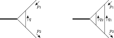
Examples of massless one-loop and two-loop scalar integrals. Thin lines represent massless scalar propagators and \(p^2_1=p^2_2= 0\)
A different \(\mu ^2\) can be used to regulate UV divergences (\(\mu ^2_\mathrm{UV}\)) and IR ones (\(\mu ^2_\mathrm{IR}\)). However, a common \(\mu ^2\) simplifies the calculation, as will be shown later. Since IR infinities are more easily understood in terms of \(\mu ^2_\mathrm{IR} > 0\), it is convenient to choose \(\mu ^2_\mathrm{UV}= \mu ^2_\mathrm{IR}= \mu ^2 > 0\).
It is instructive to study the same case in DR, where \( B^\mathrm{DR}(p^2,0,0) = \mu _\mathrm{R}^{-\epsilon } \int d^nq \frac{1}{q^2{(q+p)^2}} \). Now \(B^\mathrm{DR}(0,0,0)\) vanishes because IR and UV poles in \(\epsilon \) compensate. In fact, by introducing an arbitrary separation scale \(M\), the two divergences can be disentangled
$$\begin{aligned} { \frac{1}{(q+p)^2}}&= \frac{1}{q^2-M^2} -\bigg ( \frac{1}{q^2-M^2} -\frac{1}{(q+p)^2} \bigg ) = {\frac{1}{q^2-M^2}}\nonumber \\&-{\frac{M^2+2 (q \cdot p)}{(q^2-M^2)(q+p)^2}}. \end{aligned}$$(59)Then the integrals (\( \Delta = -\frac{2}{\epsilon }-\gamma _{E} - \ln \pi \))
$$\begin{aligned} I_\mathrm{UV}&= \mu _\mathrm{R}^{-\epsilon } \int d^nq \frac{1}{q^2 (q^2-M^2)} = i \pi ^2 \left( \Delta -\ln \frac{M^2}{\mu _\mathrm{R}^2} +1 \right) , \nonumber \\ I_\mathrm{IR}&= \mu _\mathrm{R}^{-\epsilon } \int d^nq \frac{M^2+2 (q \cdot p)}{q^2(q^2-M^2)(q+p)^2} = I_\mathrm{UV}\, \end{aligned}$$(60)cancel each other. However, this argument has a potential problem, because it requires the cancelation of two analytic continuations, \(I_\mathrm{UV}\) and \(I_\mathrm{IR}\), originally defined in domains that do not overlap [48] (\(\epsilon < 0\) and \(\epsilon > 0\)). Since no value of \(\epsilon \) exists where they are defined simultaneously, it is not obvious whether their difference represents the original function \(B^\mathrm{DR}(0,0,0)\). A possible mathematically consistent solution can be formulated in terms of modified Gaussian integrals in the \(n\)-dimensional Euclidean space [48]. In contrast, the FDR derivation in Eq. (57) is straightforward.
We use the Feynman rules of Appendix B.
Remember the discussion at the beginning of Sect. 2.4.
This implies that for each of the diagrams in Fig. 5 the routing of the momenta is chosen such that the gluon line gets the momentum \(q_{12}\). This is allowed due to the shift invariance properties of the FDR integration.
\(\delta m\big |_{\text {DR}}\) in dimensional reduction is obtained from Eq. (106) through the replacement \(\ln \mu _\mathrm{R}^2 \rightarrow \ln \mu _\mathrm{R}^2 + \Delta \), with \(\Delta \) given in footnote 21.
 in Eq. (
 , respectively, before tensor reduction.
 . In the case of closed loops,
References
J. Blumlein, PoS RADCOR2011, 048 (2011)
F. Simon, hep-ex/1401.6302 (2014)
G. Passarino, M. Veltman, Nucl. Phys. B 160, 151 (1979). doi:10.1016/0550-3213(79)90234-7
S. Frixione, Z. Kunszt, A. Signer, Nucl. Phys. B 467, 399 (1996). doi:10.1016/0550-3213(96)00110-1
S. Catani, M. Seymour, Nucl. Phys. B 485, 291 (1997). doi:10.1016/S0550-3213(96)00589-5
D.A. Kosower, Phys. Rev. D 57, 5410 (1998). doi:10.1103/PhysRevD.57.5410
J.M. Campbell, M. Cullen, E.N. Glover, Eur. Phys. J. C 9, 245 (1999). doi:10.1007/s100529900034
S. Catani, S. Dittmaier, M.H. Seymour, Z. Trocsanyi, Nucl. Phys. B 627, 189 (2002). doi:10.1016/S0550-3213(02)00098-6
Z. Nagy, D.E. Soper, JHEP 0309, 055 (2003)
Z. Bern, L.J. Dixon, D.C. Dunbar, D.A. Kosower, Nucl. Phys. B 435, 59 (1995). doi:10.1016/0550-3213(94)00488-Z
R. Britto, F. Cachazo, B. Feng, Nucl. Phys. B 725, 275 (2005). doi:10.1016/j.nuclphysb.2005.07.014
G. Ossola, C.G. Papadopoulos, R. Pittau, Nucl. Phys. B 763, 147 (2007). doi:10.1016/j.nuclphysb.2006.11.012
D. Forde, Phys. Rev. D 75, 125019 (2007). doi:10.1103/PhysRevD.75.125019
C. Berger, Z. Bern, L. Dixon, F. Febres, Cordero, D. Forde, et al. Phys. Rev. D 78, 036003 (2008). doi:10.1103/PhysRevD.78.036003
R.K. Ellis, K. Melnikov, G. Zanderighi, JHEP 0904, 077 (2009). doi:10.1088/1126-6708/2009/04/077
G. Passarino, Nucl. Phys. B 619, 257 (2001). doi:10.1016/S0550-3213(01)00528-4
P. Mastrolia, G. Ossola, JHEP 1111, 014 (2011). doi:10.1007/JHEP11(2011)014
P. Mastrolia, E. Mirabella, G. Ossola, T. Peraro, Phys. Lett. B 718, 173 (2012). doi:10.1016/j.physletb.2012.09.053
R.H. Kleiss, I. Malamos, C.G. Papadopoulos, R. Verheyen, JHEP 1212, 038 (2012). doi:10.1007/JHEP12(2012)038
S. Badger, H. Frellesvig, Y. Zhang, JHEP 1204, 055 (2012). doi:10.1007/JHEP04(2012)055
H. Johansson, D.A. Kosower, K.J. Larsen, Phys. Rev. D 87, 025030 (2013). doi:10.1103/PhysRevD.87.025030
A. Gehrmann-De Ridder, T. Gehrmann, E.N. Glover, JHEP 0509, 056 (2005). doi:10.1088/1126-6708/2005/09/056
J. Currie, A. Gehrmann-De Ridder, E. Glover, J. Pires, JHEP 1401, 110 (2014). doi:10.1007/JHEP01(2014)110
T. Binoth, G. Heinrich, Nucl. Phys. B 585, 741 (2000). doi:10.1016/S0550-3213(00)00429-6
C. Anastasiou, K. Melnikov, F. Petriello, Phys. Rev. D 69, 076010 (2004). doi:10.1103/PhysRevD.69.076010
T. Binoth, G. Heinrich, Nucl. Phys. B 693, 134 (2004). doi:10.1016/j.nuclphysb.2004.06.005
M. Czakon, Phys. Lett. B 693, 259 (2010). doi:10.1016/j.physletb.2010.08.036
S. Catani, M. Grazzini, Phys. Rev. Lett. 98, 222002 (2007). doi:10.1103/PhysRevLett.98.222002
G. ’t Hooft, M. Veltman, Nucl. Phys. B 44, 189 (1972). doi:10.1016/0550-3213(72)90279-9
R. Pittau, JHEP 1211, 151 (2012). doi:10.1007/JHEP11(2012)151
D.Z. Freedman, K. Johnson, J.I. Latorre, Nucl. Phys. B 371, 353 (1992). doi:10.1016/0550-3213(92)90240-C
F. del Aguila, A. Culatti, R. Munoz-Tapia, M. Perez-Victoria, Phys. Lett. B 419, 263 (1998). doi:10.1016/S0370-2693(97)01279-3
F. del Aguila, A. Culatti, R. Munoz, Tapia. M. Perez-Victoria. Nucl. Phys. B 537, 561 (1999). doi:10.1016/S0550-3213(98)00645-2
O. Battistel, A. Mota, M. Nemes, Mod. Phys. Lett. A 13, 1597 (1998). doi:10.1142/S0217732398001686
G. Cynolter, E. Lendvai, Central. Eur. J. Phys. 9, 1237 (2011). doi:10.2478/s11534-011-0039-y
A. Cherchiglia, M. Sampaio, M. Nemes, Int. J. Mod. Phys. A 26, 2591 (2011). doi:10.1142/S0217751X11053419
R. Pittau, Eur. Phys. J. C 74, 2686 (2014). doi:10.1140/epjc/s10052-013-2686-1
A.M. Donati, R. Pittau, JHEP 1304, 167 (2013). doi:10.1007/JHEP04(2013)167
R. Pittau, hep-ph/1305.0419 (2013)
G.F. Sterman, An Introduction to quantum field theory (Cambridge University Press, 1994)
J.C. Collins, Renormalization (Cambridge University Press, 1984)
M. Veltman, in Proceedings of the VI International Symposium on Electron and Proton Interaction at High Energies (1973), pp. 429–447
G. ’t Hooft, M. Veltman, NATO Adv. Study Inst. Ser. B Phys. 4, 177 (1974)
Z. Bern, A. De Freitas, L.J. Dixon, H. Wong, Phys. Rev. D 66, 085002 (2002). doi:10.1103/PhysRevD.66.085002
W. Siegel, Phys. Lett. B 84, 193 (1979). doi:10.1016/0370-2693(79)90282-X
Z. Bern, A. Morgan, Nucl. Phys. B 467, 479 (1996). doi:10.1016/0550-3213(96)00078-8
G. Cullen, N. Greiner, G. Heinrich, G. Luisoni, P. Mastrolia et al., Eur. Phys. J. C72, 1889 (2012). doi:10.1140/epjc/s10052-012-1889-1
G. Leibbrandt, Rev. Modern Phys. 47(4), 849 (1975)
W. Giele, E.N. Glover, D.A. Kosower, Nucl. Phys. B 403, 633 (1993). doi:10.1016/0550-3213(93)90365-V
A. Djouadi, M. Spira, J. van der Bij, P. Zerwas, Phys. Lett. B 257, 187 (1991). doi:10.1016/0370-2693(91)90879-U
J. van der Bij, M. Veltman, Nucl. Phys. B 231, 205 (1984). doi:10.1016/0550-3213(84)90284-0
Acknowledgments
This work was supported by the European Commission through contracts ERC-2011-AdG No 291377 (LHCtheory) and PITN-GA-2012-316704 (HIGGSTOOLS). We also thank the support of the MICINN project FPA2011-22398 (LHC@NLO) and the Junta de Andalucía project P10-FQM-6552.
Author information
Authors and Affiliations
Corresponding author
Appendices
Appendix A: FDR and shift invariance
In this appendix we demonstrate that, for positive integers \(\alpha \), \(\beta \), \(\gamma \), and \(\delta \),
and
where \(q_{12}= q_1+q_2\) and \(p_{12}= p_1+p_2\). Since integrals of polynomials in the integration variables vanish, the divergent parts of any one- or two-loop FDR integral can be written—after expanding in the external momenta—in terms of the four cases
In all the other cases Eqs. (110) and (111) coincide with finite integrals, for which shift invariance trivially holds.
We start proving Eq. (110) with \(\alpha = 1\). By using the shorthand notation
one writes the FDR expansions of the two sides of the equation as
Then
where the shift invariance of the dimensionally regulated integrals over \(1/\bar{D}\) and \(1/\bar{q}^2\) has been used. By expanding the last integrand one obtains
Since the l.h.s. of Eq. (116) vanishes upon integration at any order in \(p\), the same happens for the combination
The last integral in Eq. (115) can then be rewritten as
so that
which proves Eq. (110) with \(\alpha = 1\). The case \(\alpha = 2\) is proven by taking the derivative of Eq. (119) with respect to \(m^2\).
We now deal with the case \(\beta = \gamma = \delta = 1\). The FDR expansion of the l.h.s. of Eq. (111) is given by Eq. (8). As for the r.h.s., we introduce
in terms of which the expansion reads
Then, by rewriting
and shifting all the \(\bar{D}_i\) and the quadratically divergent integrals, Eq. (8) produces
An expansion up to \(\mathcal{O}(p^2_1)\), \(\mathcal{O}(p^2_2)\), and \(\mathcal{O}(p_1 p_2)\) of the second line and of the terms
in the last three lines produces extra integrands which—by the same argument used at one loop—vanish upon integration. The addition of such terms reconstructs \(J^\prime _{\mathrm{F},2}(q_1,q_2)\) as given in Eq. (121), so that
Finally, taking the derivative with respect to \(m^2_{12}\) demonstrates the last case.
With more loops the proof follows the same reasoning: the mismatch between the FDR expansion of shifted and unshifted integrands is cured by vanishing integrals obtained by expanding the polynomially divergent integrals in \(J_\mathrm{INF}(q_1,\ldots , q_\ell )\) at the relevant order in \(p\), as in Eq. (116).
Appendix B: Feynman rules
For completeness we list, in Fig. 8, the Feynman rules used in the calculation. \(Q_t\), \(m_0\) and \(v\) are the top quark charge, the top bare mass and the vacuum expectation value of the Higgs field, respectively.

Feynman rules used in the computation of \(H \rightarrow \gamma \gamma \) at \({\mathcal {O}}(\alpha _S)\)
Appendix C: A few FDR defining expansions
We collect here the two-loop FDR defining expansions used throughout the paper. Denominators are defined in Eq. (7) and divergent integrands are written in square brackets.
-
1.
Expansion for \(\displaystyle \int [d^4q_1][d^4q_2] \frac{q^\alpha _1 q^\beta _1}{\bar{D}^3_1 \bar{D}_2 \bar{D}_{12}}\):
$$\begin{aligned}&\frac{q^\alpha _1 q^\beta _1}{\bar{D}^3_1 \bar{D}_2 \bar{D}_{12}} = q^\alpha _1 q^\beta _1 \left\{ \left[ \frac{1}{\bar{q}^6_1 \bar{q}^2_2 \bar{q}^2_{12}} \right] \right. \nonumber \\&\quad +\left( \frac{1}{\bar{D}^3_1} -\frac{1}{\bar{q}_1^6}\right) \left( \left[ \frac{1}{\bar{q}_2^4}\right] -\frac{q_1^2+2(q_1 \cdot q_2)}{\bar{q}_2^4 \bar{q}_{12}^2} \right) \nonumber \\&\quad +\left. \frac{1}{\bar{D}_{1}^3 \bar{q}_2^2\bar{D}_{12} } \left( \frac{m_2^2}{\bar{D}_{2}}+\frac{m_{12}^2}{\bar{q}_{12}^2} \right) \right\} . \end{aligned}$$(125) -
2.
Expansion for \(\displaystyle \int [d^4q_1][d^4q_2] \frac{1}{\bar{D}^2_1 \bar{D}_2 \bar{q}^2_{12}}\):
$$\begin{aligned} \frac{1}{\bar{D}^2_1 \bar{D}_2 \bar{q}^2_{12}}&= \left[ \frac{1}{\bar{q}^4_1 \bar{q}^2_2 \bar{q}^2_{12}} \right] +\left( \frac{m^2_1}{\bar{D}_1 \bar{q}_1^4}+\frac{m^2_1}{\bar{D}^2_1 \bar{q}_1^2} \right) \nonumber \\&\times \left( \left[ \frac{1}{\bar{q}_2^4}\right] -\frac{q_1^2+2(q_1 \cdot q_2)}{\bar{q}_2^4 \bar{q}_{12}^2} \right) \nonumber \\&+ \frac{m_2^2}{\bar{D}^2_1 (\bar{D}_2\bar{q}^2_2) \bar{q}^2_{12}}. \end{aligned}$$(126) -
3.
Expansion for \(\displaystyle \int [d^4q_1][d^4q_2] \frac{q^\alpha _1 q^\beta _1}{\bar{D}^2_1 \bar{D}^2_2 \bar{q}^2_{12}}\):
$$\begin{aligned} \frac{q^\alpha _1 q^\beta _1}{\bar{D}^2_1 \bar{D}^2_2 \bar{q}^2_{12}}&= q^\alpha _1 q^\beta _1 \left\{ \left[ \frac{1}{\bar{q}^4_1 \bar{q}^4_2 \bar{q}^2_{12}} \right] + \left( \frac{m^2_2}{\bar{D}_2 \bar{q}_2^4}+\frac{m^2_2}{\bar{D}^2_2 \bar{q}_2^2} \right) \right. \nonumber \\&\times \left. \left( \left[ \frac{1}{\bar{q}_1^6}\right] -\frac{q_2^2+2(q_1 \cdot q_2)}{\bar{q}_1^6 \bar{q}_{12}^2} \right) \right. \nonumber \\&+\left. \left( \frac{1}{\bar{D}^2_1} - \frac{1}{\bar{q}_1^4} \right) \frac{1}{\bar{D}_{2}^2 \bar{q}_{12}^2 } \right\} . \end{aligned}$$(127) -
4.
Expansion for \(\displaystyle \int [d^4q_1][d^4q_2] \frac{q^\alpha _{12} q^\beta _{12}}{\bar{D}^2_1 \bar{D}^2_2 \bar{q}^2_{12}}\):
$$\begin{aligned} \frac{q^\alpha _{12} q^\beta _{12}}{\bar{D}^2_1 \bar{D}^2_2 \bar{q}^2_{12}}&= q^\alpha _{12} q^\beta _{12} \left\{ \left[ \frac{1}{\bar{q}^4_1 \bar{q}^4_2 \bar{q}^2_{12}} \right] +\left[ \frac{1}{\bar{q}_{12}^6}\right] \left( \left( \frac{m^2_1}{\bar{D}_1 \bar{q}_1^4}\right. \right. \right. \nonumber \\&\left. \left. +\frac{m^2_1}{\bar{D}^2_1 \bar{q}_1^2} \right) + \left( \frac{m^2_2}{\bar{D}_2 \bar{q}_2^4}+\frac{m^2_2}{\bar{D}^2_2 \bar{q}_2^2} \right) \right) \nonumber \\&\left. + \frac{1}{\bar{q}^2_{12}} \left( \left( \frac{1}{\bar{D}^2_1} - \frac{1}{\bar{q}_1^4} \right) \left( \frac{1}{\bar{D}^2_2} - \frac{1}{\bar{q}_2^4}\right) \right. \right. \nonumber \\&+ \left( \frac{1}{\bar{q}^4_1} - \frac{1}{\bar{q}^4_{12}} \right) \left( \frac{1}{\bar{D}^2_2} - \frac{1}{\bar{q}_2^4} \right) \nonumber \\&\left. \left. + \left( \frac{1}{\bar{q}^4_2} - \frac{1}{\bar{q}^4_{12}} \right) \left( \frac{1}{\bar{D}^2_1} - \frac{1}{\bar{q}_1^4} \right) \right) \right\} . \end{aligned}$$(128)
Appendix D: The basic two-loop scalar integral
In this appendix, we demonstrate that the basic two-loop scalar integral in Eq. (95) reads
with
A direct integration of the finite part of its FDR defining expansion—Eq. (126)—gives
where
By power counting—due to the presence of \({1}/{q^4_i}\) terms—a logarithmic dependence on \(\mu \) is expected in \(I_1(m_1)\), while \(\mu \) can be immediately set to zero in \(I_2(m_1,m_2)\). A natural split is then obtained in FDR: \(I_2(m_1,m_2)\) only depends on
and \(I_1(m_1)\) on
so no difficult integral containing both ratios needs to be computed. A simple Feynman parametrization produces
and
from which Eq. (129) follows. The same result can be derived as a finite combination of divergent integrals. From Eq. (126), by using DR,
The relevant DR integrals can be found in the appendix of [51].
Rights and permissions
Open Access This article is distributed under the terms of the Creative Commons Attribution License which permits any use, distribution, and reproduction in any medium, provided the original author(s) and the source are credited.
Funded by SCOAP3 / License Version CC BY 4.0.
About this article

Cite this article
Donati, A.M., Pittau, R. FDR, an easier way to NNLO calculations: a two-loop case study. Eur. Phys. J. C 74, 2864 (2014). https://doi.org/10.1140/epjc/s10052-014-2864-9
Received:
Accepted:
Published:
DOI: https://doi.org/10.1140/epjc/s10052-014-2864-9