Invited Review: Short-term Variability with the Observations from the Helioseismic and Magnetic Imager (HMI) Onboard the Solar Dynamics Observatory (SDO): Insights into Flare Magnetism

Abstract

Continuous vector magnetic-field measurements by the Helioseismic and Magnetic Imager (HMI) onboard the Solar Dynamics Observatory (SDO) allow us to study magnetic-field properties of many flares. Here, we review new observational aspects of flare magnetism described using SDO data, including statistical properties of magnetic-reconnection fluxes and their rates, magnetic fluxes of flare dimmings, and magnetic-field changes during flares. We summarize how these results, along with statistical studies of coronal mass ejections (CMEs), have improved our understanding of flares and the flare/CME feedback relationship. Finally, we highlight future directions to improve the current state of understanding of solar-flare magnetism using observations.

1 Introduction

The Standard CSHKP Flare Model, arcade–arcade reconnection (Figure 1): The traditional, two-dimensional (2D) model of the solar flare, called CSHKP (Carmichael, 1964; Sturrock, 1968; Hirayama, 1974; Kopp and Pneuman, 1976), and its extension to three dimensions (3D, Longcope et al., 2007; Aulanier, Janvier, and Schmieder, 2012; Aulanier et al., 2013; Janvier, Démoulin, and Dasso, 2014; Savcheva et al., 2015, 2016) describe the following general scenario. Magnetic reconnection occurs under a pre-existing rising flux rope or a sheared arcade (gray twisted field lines in Figure 1; van Ballegooijen and Martens, 1989; Longcope et al., 2007; Priest and Longcope, 2017; Li et al., 2020; Patsourakos et al., 2020) between pairs of arcade field lines. As a result, a set of closed field lines and an expanding flux rope form below and above the reconnection site, respectively. This “flare reconnection” both adds flux to the incipient CME and leads to the acceleration of non-thermal flare particles (e.g. Fletcher and Hudson, 2008). When these particles interact with the denser plasma of the upper chromosphere they emit X-rays via bremsstrahlung, first heating and then evaporating that plasma (Fisher, Canfield, and McClymont, 1985). Both this bremsstrahlung and chromospheric heating are observable, the former in hard X-rays and the latter in chromospheric brightenings (in H$\upalpha$ and other wavelengths) referred to as flare ribbons (Cheng et al., 1983; Doschek et al., 1983). Chromospheric plasma evaporated by the high-energy flare particles supplies the emission measure that makes post-flare loops visible in coronal EUV and soft X-ray images. Figure 1 shows a cartoon of the 3D CSHKP model with the main large-scale observational properties that it explains: an expanding flux rope that forms the core of the coronal mass ejection (CME), cusp-shaped post-reconnection field lines, core and secondary coronal dimmings, flare ribbons, and post-reconnection field lines that form the flare arcade. Note that the magnetic field in the reconnection region typically contains a significant guide field (e.g. Qiu et al., 2017), associated with a component of the field (its shear component) along the polarity-inversion line (PIL). As the flux rope above the reconnection site rises, the reconnection site proceeds to higher altitudes, and the ribbons move away from the PIL. As the flux rope expands, it stretches the overlying magnetic-field lines, causing the coronal volume around the flux-rope and overlying-field footpoints to become depleted in density. This density depletion leads to formation of transient darkenings or coronal dimmings (Hudson, Acton, and Freeland, 1996; Thompson et al., 2000). Dimmings at flux-rope footpoints and footpoints of overlying field lines are called core and secondary dimmings, respectively. In this model, the footpoints of the flux rope remain fixed.

Figure 1

The 3D CSHKP flare model and beyond. Green and dark blue arcade field lines reconnect in an arcade–arcade reconnection below the gray expanding flux rope forming a yellow cusped field line below and a red twisted line around the flux rope. The footpoints of the newly reconnected field lines form flare ribbons. The footpoints of the expanding flux rope and the stretched overlying arcade correspond to core and secondary dimmings, respectively. Beyond the standard scenario, when flux-rope and arcade field lines reconnect in the flux-rope–arcade reconnection, additional flare ribbons form and the flux-rope’s footpoints drift.

Extended CSHKP model, flux-rope–arcade reconnection (Figure 1): In addition to the above CSHKP model, where reconnection occurs between fields that wrap around the rising flux rope (the so-called “arcade–arcade” reconnection in Figure 1), reconnection can occur between the flux rope and surrounding fields (the “flux-rope–arcade” reconnection in Figure 1) or within the flux rope (Dudík et al., 2019; Aulanier and Dudík, 2019). Dudík et al. (2019), Zemanová et al. (2019), and Aulanier and Dudík (2019) presented several Solar Dynamics Observatory (SDO: Pesnell, Thompson, and Chamberlin, 2012) flare observations where these scenarios create a new flux-rope field line and a flare loop, causing the flux-rope erosion (see schematic representation of this case on the right side of Figure 1). Aulanier and Dudík (2019) performed an idealized MHD simulation to explain these observations via reconnection between the flux rope and arcade fields that surround it. A systematic, observational survey of ribbon evolution would be useful to understand how frequently this scenario occurs on the Sun.

Standard Flare Model Observables: Flare reconnection vs. CME properties: The CSKHP scenario shown in Figure 1 provides not only a general qualitative concept of how a two-ribbon eruptive flare occurs but also a quantitative framework to relate flares to CMEs.

First, the CSHKP model implies a quantitative relationship between the reconnection flux in the corona and the magnetic flux swept by the flare ribbons (the ribbon flux, e.g., Forbes and Priest, 1984; Poletto and Kopp, 1986):

$$ \frac{\partial \Phi _{\mathrm{cor}}}{\partial t} = \frac{\partial}{\partial t} \int B_{\mathrm{cor}} \, \mathrm{d}S_{\mathrm{cor}} = \frac{\partial \Phi _{\mathrm{ph}}}{\partial t} = \frac{1}{2} \frac{\partial}{\partial t} \int |B_{\mathrm{n}}| \, \mathrm{d}S_{\mathrm{rbn}}~. $$

(1)

The left-hand side $[\partial \Phi _{\mathrm{cor}}/\partial t]$, denotes the coronal magnetic reconnection rate as reconnection flux per unit time defined by the integration of the (ideally) inflowing coronal magnetic field’s reconnecting component $[B_{\mathrm{cor}}]$ over the reconnection area $[\mathrm{d}S_{\mathrm{cor}}]$ that is bounded by the curve $\mathcal{C}$, outside of which the evolution is ideal (i.e. $\boldsymbol{E} = -(\boldsymbol{v} \times \boldsymbol{B})$/c). On the right-hand side, $B_{\mathrm{n}}$ is the normal component of the magnetic field within the ribbons in the photosphere. While direct measurements of $B_{\mathrm{cor}}$ and d$S_{\mathrm{cor}}$ in the corona are not currently feasible, $B_{\mathrm{n}}$ and d$S_{\mathrm{rbn}}$ are relatively straightforward to obtain from photospheric magnetogram and lower-atmosphere flare-ribbon observations. Summing the total photospheric normal flux $[\Phi _{\mathrm{ph}}]$ swept by the flare ribbons,

$$ \Phi _{\mathrm{rbn}} \equiv \int \left | \frac{\partial \Phi _{\mathrm{ph}}}{\partial t} \right | \mathrm{d}t = \frac{1}{2} \int |B_{\mathrm{n}}| \mathrm{d}S_{\mathrm{rbn}} ~, $$

(2)

gives an indirect, but well-defined, measure of the amount of magnetic flux processed by reconnection in the corona during the flare. According to the CSHKP model in the nomenclature adopted by Qiu et al. (2007), this reconnected flux should correspond to the eruption’s poloidal flux.

Secondly, the 3D CSHKP model implies a quantitative relationship between coronal dimmings and the axial flux in the flux rope, which has been referred to as the rope’s toroidal flux (Qiu et al., 2007):

$$ \Phi _{\mathrm{dim}} \equiv \frac{1}{2} \int |B_{\mathrm{n}}| \, \mathrm{d}S_{\mathrm{dim}} ~. $$

(3)

Here, the integral sums the photospheric / chromospheric magnetic fields underlying volumes whose EUV dimmed as a result of the eruption.

Some statistical studies before SDO: Since the 1990s, observational efforts have been made to link interplanetary CME (ICMEs) and magnetic-cloud (MC) properties to various solar progenitors, including flare ribbons, coronal dimmings, SXR fluxes, etc. To list a few results, reports have associated UV and HXR emission with the acceleration of filament eruptions (Jing et al., 2005; Qiu et al., 2004); CME acceleration with flare-energy release (Zhang and Low, 2001; Zhang and Dere, 2006); GOES flare class and flare-reconnection flux with CME speed and flux content of the interplanetary CMEs (e.g. Qiu and Yurchyshyn, 2005; Qiu et al., 2007; Miklenic, Veronig, and Vršnak, 2009). In most of these analyses, the underlying data for the flare ribbon/dimming properties were of limited accuracy and involved different sets of instruments observing in different wavelengths, which required time-consuming co-alignment and inter-calibration, making systematic comparison of flare-ribbon properties difficult for large numbers of events.

Launch of SDO with the Helioseismic and Magnetic Imager (HMI: Scherrer et al., 2012; Hoeksema et al., 2014) and the Atmospheric Imaging Assembly (AIA: Lemen et al., 2012) instruments, represented the first time that both a vector magnetograph and ribbon-imaging capabilities became available on the same observing platform, making co-registration of AIA and HMI full-disk data relatively easy. This new capability, along with over a decade of continuous observations of the whole solar disk, led to a rise of statistical studies comparing various flare and CME properties.

The goal of this review is to summarize recent observations of the short-term transient variability of active-region magnetic fields before flares as well as their changes during the flare, primarily using the observations from HMI and other instruments. Most recent reviews on flare–CME magnetism, such as that by Schmieder, Aulanier, and Vršnak, 2015, came out before we had large statistical studies of flare magnetic properties. Our aim is to fill this gap. For other flare-related topics, see a review of pre-flare magnetic-field properties, including the 3D coronal field structure, by Patsourakos et al. (2020); a review of the origins, early evolution, and predictability of solar eruptions by Green et al. (2018); overviews of numerical simulations, including data-driven simulations, by Janvier, Aulanier, and Démoulin (2015), Hayashi et al. (2018), Toriumi and Wang (2019); and overviews of the current understanding of CMEs, by Zhang et al. (2021) and Temmer (2021).

The article is organized as follows: In Section 2, we describe flare-ribbon-reconnection fluxes. In Section 3 we discuss near-Sun flux-rope properties, as determined from flare dimmings. In Section 4 we discuss flare-associated magnetic-field changes, and in Section 5 we discuss flare versus CME properties, including comparisons of eruptive and confined events. Finally, in Section 6 we draw conclusions and highlight future prospects.

2 Flare Ribbons: Footpoints of Reconnected Fields

Although magnetic reconnection originating in a thin current sheet (or multiple sheets) in the corona is believed to be crucial in flare-energy partition, its nature and the processes leading to its onset are not yet fully understood. Apart from a few observations on the limb (Warren et al., 2018; French et al., 2019; Chen et al., 2020), current sheets are difficult to observe directly. Flare ribbons below erupting coronal structures are understood to be the chromospheric footpoints of reconnecting coronal fields. Hence, their spatial and temporal properties could be used to probe reconnection in the current sheet. In this section, we review recent progress on flare magnetic properties learnt from flare ribbons.

Two stages of ribbon motion (Figure 2): Flare ribbons’ motion commonly exhibits two stages: parallel and perpendicular to PIL (Su, Golub, and Van Ballegooijen, 2007; Qiu, 2009; Qiu et al., 2010; Cheng et al., 2012).

Figure 2

Two stages of ribbon motion (Qiu, 2009). Left: Michelson Doppler Imager (MDI) / Solar and Heliospheric Observatory (SOHO) photospheric magnetogram with the contours of MDI magnetic cells (dotted lines) and the cumulative TRACE flare-ribbon area (solid olive color). “P” and “N” denote positive and negative magnetic cells, respectively. Middle: Temporal and spatial evolution of the flare-ribbon area with contours of the MDI magnetic cells. Color corresponds to ribbon position at a certain time: the first parallel stage (dark blue) is followed by the second perpendicular or “main” stage (green–red). At 15:54 UT, the flare ribbons are in the light-blue areas, which roughly divide two stages. Right: temporal profiles of the total reconnection flux (thin solid line) and the reconnection rate (thick solid line) in the positive and negative polarities, respectively. Thin dashed and dotted lines show normalized GOES soft X-ray flux and its temporal derivative, respectively. The thick dashed vertical bar at 54 minutes indicates the division between two ribbon stages. See Section 2 for details. Reproduced with the author’s permission.

Parallel stage of ribbon motion: During the first stage, the flare-ribbon brightening starts and primarily spreads along the PIL, with brightenings in the two polarities proceeding either in opposite directions (“bidirectional”, Li and Zhang 2009) or the same direction, from one end of the PIL to the other in zipper reconnection (Qiu et al., 2017). In many flares with bidirectional motions, brightenings proceed from high to low shear angles (e.g. Su, Golub, and Van Ballegooijen, 2007), i.e. from separations that are more parallel to PIL to separations that are more perpendicular to PIL. Using MHD simulations, Dahlin et al. (2021) showed that this high-to-low shear transition seen at the footpoints is co-temporal with a decrease in the coronal guide field. High-to-low shear evolution also leads to transition of the reconnecting fields from initially more toroidal to more poloidal. However, ribbon evolution in many events is more complex (e.g. Yang et al., 2009), meaning it can be difficult to determine any systematic change in shear, or to discern parallel-type progression of brightenings. The maximum apparent speeds of parallel brightenings’ propagation are up to $v_{\mathrm{parallel}}\approx 150\mbox{ km}$ s⁻¹, on the order of expected active-region chromospheric Alfvén speeds, but below the expected coronal active-region Alfvén speed (see Qiu et al., 2017 and references therein).

Perpendicular or “main” stage of ribbon motion: During the second perpendicular or “main phase”, ribbons primarily move away from the PIL more slowly, at up to $v_{\mathrm{perp}}\approx$ 60 km s⁻¹ (Hinterreiter et al., 2018). Recently, however, Dudík et al. (2019), Zemanová et al. (2019), and Aulanier and Dudík (2019) noted that ribbons’ main-stage evolution can be more complex: they found that some ribbons move toward the PIL instead of away from it. They argue that this motion corresponds to reconnection between the expanding flux-rope field lines and surrounding, closed field lines (see flux-rope–arcade reconnection in Figure 1). In general, ribbon speeds and magnetic fields in conjugate footpoints provide an estimate of the ratio between the guide field and the reconnection field in the coronal current sheet (Qiu et al., 2010), therefore statistical analysis of a larger number of ribbons would be helpful to provide a general description of the flare guide field.

Ribbons as signatures of flux-rope formation: Priest and Longcope (2017) investigated parallel to PIL motion (zipper) reconnection in two scenarios, starting from either a sheared arcade or a pre-existing flux rope, which should yield different amounts of twist in the resulting ejection. Starting from a sheared arcade, they proposed that first the zipper reconnection creates a twisted flux rope of roughly one turn, then the main-phase perpendicular reconnection builds up the bulk of the erupting flux rope with a relatively uniform twist of a few turns. Starting from a pre-existing flux rope, they proposed that zipper reconnection could create a core with many turns, then the main-phase reconnection adds a layer of roughly uniform twist to the more highly twisted central core. This scenario could explain the observations of Hu et al. (2014), who found that some ropes had a moderate twist that was uniformly distributed from their cores to their edges, while others had highly twisted cores surrounded by more weakly twisted fields.

Ribbon Fine Structure (Figure 3): Observations of flare ribbons show significant fine structure in the form of knots, wave-like perturbations, and spirals that evolve as the flare progresses (e.g. Dudík et al., 2016; Brannon, Longcope, and Qiu, 2015; Parker and Longcope, 2017). Figure 3 shows an example of ribbons’ fine structure as observed by the Interface Region Imaging Spectrograph (IRIS: De Pontieu et al., 2014). The origin of these structures is not well understood. One possibility is that they are related to the tearing instability in the flare current sheet. Wyper and Pontin (2021) used an analytical 3D magnetic field to show that there is a direct link between flare-ribbon fine structure and flare current-sheet tearing, with the majority of the ribbon fine structure related to oblique tearing modes. Another possibility is the Kelvin–Helmholtz (KH) instability, which occurs at a fluid interface with a discontinuity in flow speeds (see Brannon, Longcope, and Qiu, 2015 and references therein). Temporal analysis of the widths of flare ribbons suggests that flare reconnection is patchy and highly intermittent (Naus et al., 2022), consistent with models based on coronal observations of post-flare loops (Linton and Longcope, 2006).

Figure 3

Ribbon fine structure (Wyper and Pontin, 2021) as observed by IRIS: observations of the 2014 September X-class flare ribbons with spiral and wave-like patterns. See Section 2 for details. Reproduced with the author’s permission.

Ribbons’ Power Spectrum: In addition to direct spatial analysis of the ribbon structure, investigating the power spectra in the spatial domain along the ribbon might provide insight into processes across the current sheet, perpendicular to the magnetic field. French et al. (2021) used high-cadence (1.7 second) IRIS observations of ribbons in a B-class flare to analyze the evolution of the ribbons’ spatial scales resulting from cross-sheet dynamics. Combining temporal evolution of the spatial power spectrum of flare ribbons with Si iv non-thermal velocities, they proposed a scenario for the flare-onset timeline. In this scenario, the flare starts with an exponential growth at a key spatial scale, which is interpreted as a signature of tearing-mode instability onset. This instability then triggers a cascade and an inverse cascade to smaller and larger spatial scales simultaneously towards a power spectrum consistent with plasma turbulence. Observed combination of cascades is suggested to originate from the interplay of magnetic-island collapse and coalescence. With higher spatial resolution from new telescopes, such as the Daniel K. Inouye Solar Telescope (DKIST: Rimmele et al., 2020), we would be able to measure the power at smaller spatial scales, allowing further comparison with tearing-mode theory.

2.1 Flare Ribbons: Statistical Properties (Table 1 and Figure 4)

While individual studies of flare temporal and spatial characteristics are highly valuable, one of the major strengths of the SDO data is large-number studies. In Table 1 we summarize recent statistical results analyzing flare-ribbon magnetic-reconnection properties with other flare properties primarily using SDO data.

Table 1 Magnetic-reconnection properties from flare ribbons: overview of statistical works summarizing the range of flare peak X-ray flux [$X$] and the 20th to 80th percentile range [$X_{\mathrm{rbn}}[P_{20},P_{80}]$] for flare-ribbon magnetic reconnection flux [$\Phi _{\mathrm{rbn}}$], mean magnetic flux density [$\bar{B}_{\mathrm{rbn}}$], ribbon area [$A_{\mathrm{rbn}}$], fraction of the reconnected magnetic flux [$R_{\Phi}$], reconnection electric field [$E_{\mathrm{rbn}}$], and correlation coefficients between different variables [$r_{\mathrm{s}}$], where $\dot{\Phi}_{\mathrm{rbn}}$ is the peak reconnection flux rate and $\dot{X}$ is the peak value of the temporal derivative of the GOES X-ray flux in the 1 – 8 Å channel. See Section 2.1 for details.

What have we learnt about magnetic reconnection from over a decade of ribbon observations with SDO?

• Typical range of reconnection fluxes: We now know that flare-reconnection fluxes range within the 20th to 80th percentile of $\Phi _{\mathrm{rbn}}[P_{\mathrm{20}},P_{\mathrm{80}}]=[54,210]\times 10^{20}$ Mx involving $R_{\Phi}[P_{\mathrm{20}},P_{\mathrm{80}}]=[1.3,5.1]\%$ of the overall AR magnetic flux.

• Correlation between the flare peak X-ray flux: We learnt that the reconnection flux and its rate of change are direct signatures of the energy-release process. A vivid illustration of that is the strong correlation between the flare-peak X-ray flux with the ribbon-reconnection flux (see Figure 4, middle panel). Using 1600-Å observations, Kazachenko et al. (2017) and Toriumi et al. (2017) found the Spearman correlation coefficient between actual values (or a Pearson correlation coefficient in the log–log space) of $r_{\mathrm{s}}(\Phi _{\mathrm{rbn}},X)=0.7$. Using H$\upalpha$, Tschernitz et al. (2018) found an even stronger correlation of $r_{\mathrm{s}}(\Phi _{\mathrm{rbn}},X)=0.9$. Tschernitz et al. (2018) also found a strong correlation between the peak reconnection rate and GOES/SXR derivative (see Figure 4 right panel): $r_{\mathrm{s}}(\dot{\Phi}_{\mathrm{rbn}},\dot{X})=0.9$. These correlations are much larger than the correlation between the peak X-ray flux and the total AR magnetic flux: $r_{\mathrm{s}}(\Phi _{\mathrm{AR}},X)=0.2$ (Kazachenko et al., 2017, Figure 4, left panel). One possibility to explain the differences in the correlation coefficient using 1600 -Å and H$\upalpha$ data is the different physics of 1600 -Å and H$\upalpha$ spectral-line formation. Sindhuja et al. (2019) compared Kanzelhöhe Solar Observatory (KSO) ribbon images in H$\upalpha$ and Ca K and found that the H$\upalpha$ signal “follows the trend of GOES/SXR” while SDO/AIA 1600 Å and Ca K “follow the trend of GOES/SXR derivative.” Sindhuja et al. (2019) also compared ribbon-reconnection fluxes with the GOES flare fluence (time integrated SXR light curve: $F_{\mathrm{GOES}}$), finding that the reconnection flux has an even stronger correlation with fluence than with the peak X-ray flux: $r_{\mathrm{s}}(\Phi _{\mathrm{rbn}},F_{\mathrm{GOES}})=0.8$ vs. $r_{\mathrm{s}}(\Phi _{\mathrm{rbn}},X)=0.6$ (for their sample). This result is sensible, since fluence and reconnection flux represent cumulative flare-energy products. The power-law relationship between the peak X-ray flux and the ribbon-reconnection flux could be described as $X\propto \Phi ^{1.5}_{\mathrm{rbn}}$ (Kazachenko et al., 2017). This exponent value is consistent with the Warren and Antiochos (2004) scaling law derived from hydrodynamic simulations of impulsively heated flare loops, thus indicating that the energy released during the flare as soft X-ray radiation originates from the free magnetic energy stored in the magnetic field released during reconnection. Similar scaling laws have been explored by many authors in more recent studies (Reep, Bradshaw, and McAteer, 2013; Warmuth and Mann, 2016; Reep and Knizhnik, 2019; Aschwanden, 2020; Qiu, 2021).

  Figure 4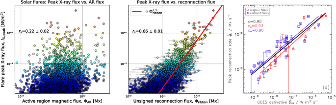

  

  Ribbons’ statistical properties: Left and Middle: Scatter plots of peak X-ray flux vs. unsigned AR magnetic flux and flare-reconnection flux (Kazachenko et al., 2017). Right: peak reconnection rate vs. GOES/SXR flux peak derivative (Tschernitz et al., 2018). See Section 2.1 for details. Reproduced with the author’s permission.

• Reconnection flux fractions vs. peak X-ray fluxes: Another SDO discovery is a moderate correlation between the flare-peak X-ray flux and the fraction of the reconnected flux: $r_{\mathrm{s}}(R_{\Phi},X)=0.5$ (Kazachenko et al., 2017; Toriumi et al., 2017). This correlation could be a consequence of the strong correlation between the flare peak X-ray flux and the reconnection flux.

• Ribbon-separation distances vs. coronal electric fields: Peak X-ray flux correlates with ribbon-separation distances [$D_{\mathrm{rbn}}$] and coronal electric-field strengths [$E_{\mathrm{rbn}}$] (Hinterreiter et al., 2018): $r_{\mathrm{s}}(D_{\mathrm{rbn}},X)=0.3$, $r_{\mathrm{s}}(E_{\mathrm{rbn}},X)=0.5$ for confined and $r_{\mathrm{s}}(D_{\mathrm{rbn}},X)=0.6$, $r_{\mathrm{s}}(E_{\mathrm{rbn}},X)=0.8$ for eruptive events. These results indicate that stronger flares have ribbons separating further away and are also associated with larger coronal electric fields. Weak correlation between the peak ribbon-separation speed and the X-ray flux has been found: $r_{\mathrm{s}}(V_{\mathrm{rbn,max}},X)=[0.2,0.3]$ (Hinterreiter et al., 2018).

• Flare durations vs. ribbon properties: Toriumi et al. (2017) and Reep and Knizhnik (2019) have also investigated the relationship between the ribbon properties and flare duration. Reep and Knizhnik (2019) found that flare duration is independent of peak X-ray flux, but it is correlated with magnetic reconnection flux and ribbon area for strong X-class flares: $r_{\mathrm{s}}(\Phi _{\mathrm{rbn}},t_{\mathrm{GOES}})=[0.5,0.8]$, for M- and X-class flares, respectively. On the other hand, weaker flares’ durations are independent of the reconnection flux. The lack of correlation for weaker flares might be due to large measurement errors or differences in the physical processes driving the weak and large flares.

Summary (Flare Ribbons): Footpoints of newly reconnected field lines seen as flare ribbons tell us about the properties of the magnetic reconnection above in the current sheet that are otherwise unobservable. Spatial analysis of flare ribbons suggests that ribbons typically evolve first parallel and then perpendicular to the PIL, providing proxies for the guide-to-reconnection-field ratios in the overlying field. These two stages contribute differently to the flux-rope formation process. Simulations suggest that ribbons’ fine structure is related to the oblique tearing mode of the current sheet above. Analysis of the ribbon power spectrum for one event also suggests that the flare starts as a result of the tearing-mode instability that then triggers a cascade towards the plasma turbulence. Analysis of thousands of cumulative flare-ribbon areas suggests that the amount of flux reconnected during a flare is related to the flare’s SXR irradiance, and that the flare-ribbon area is related to the flare’s duration, at least for large X-class events. As of now, most of the many-event studies have focused on ribbons’ cumulative properties, ignoring the details of the spatial and temporal evolution; in contrast, studies of ribbons’ fine structure and evolution focused on single events. Therefore, we suggest that a large advance in the field could be gained by statistical studies of ribbons’ temporal and spatial properties, to understand the details of the dynamics of the current sheet above as well as parameter ranges for different events.

3 Coronal Dimmings: Footpoints of Expanding Coronal Structures

Coronal dimmings are regions of decreased emission (Figure 5) in the extreme-ultraviolet (EUV) and soft X-ray (SXR) regions. They were first observed by Skylab (Rust, 1983) and are now typically observed on the Sun with the Extreme Ultraviolet Variability Experiment (SDO/EVE) (Mason et al., 2016, 2019), SDO/AIA 211 Å (Dissauer et al., 2018), 193 Å (Krista and Reinard, 2017), 171 Å, etc. lines, and on other stars (Veronig et al., 2021, see Figure 5). Cheng and Qiu (2016) presented a nice overview of possible dimming mechanisms. Dimmings are caused by a density decrease due to rapid expansion of the CME structure and overlying fields (Tian et al., 2012; Cheng and Qiu, 2016). More than half of dimmings occur within ≈ five minutes of the flare onset (Dissauer et al., 2018), with more than $80\%$ of dimmings occurring within ten minutes. Weaker gradual dimmings sometimes occur before the flare onset, marking a slow rise of the flux rope (Qiu and Cheng, 2017; Zhang, Su, and Ji, 2017; Prasad et al., 2020). Differential emission measure (DEM) analysis of coronal dimmings shows that the impulsive-emission decrease in dimming regions stems mostly from a drop in density with small temperature variations. Cheng and Qiu (2016) found a linear relationship between coronal-dimming depth and the radial expansion ratio of the CME suggesting that the expansion of the CME follows a 1D isothermal expansion. Spectroscopic studies confirmed the presence of outflowing plasma in the dimming regions (Harra and Sterling, 2001; Miklenic et al., 2011; Tian et al., 2012; Veronig et al., 2019) with velocities decreasing with time (Jin et al., 2019).

Figure 5

Coronal dimming example on 7 March 2012 from Veronig et al. (2021). Columns a and b: SDO/AIA 193 Å direct and logarithmic base-ratio images showing the flare and coronal dimming areas (black arrows). The red box shows the region used to calculate the flare light curve (Panel d). The color bar above Column b shows intensity changes with respect to the pre-event emission. Column c: CMEs imaged by the Solar Terrestrial Relations Observatory / Extreme Ultraviolet Imager (STEREO-B/EUVI) and COR2 white-light coronagraphs. Three rows correspond to three different times. The red contours outline the CME fronts. d, Top: spatially resolved SDO/AIA 19.3 -nm light curves of the flare (red curve) and dimming region (blue curve). d, Middle: SDO/EVE 15 – 25 nm broadband Sun-as-a-star light curve. The horizontal dashed line indicates a $0\%$ relative difference. d, Bottom: pre-event subtracted SDO/EVE irradiance spectra over ten minutes during the flare peak (red) and over the maximum dimming depth (blue), as indicated by orange and blue vertical lines and shaded regions in the middle panel. See Section 3 for details. Reproduced with the author’s permission.

3.1 Coronal Dimmings: Statistical Properties (Table 2)

Coronal dimmings: main properties: Dissauer et al. (2018), Krista and Reinard (2017), and Aschwanden et al. (2017) presented the largest-sample morphological studies of dimmings to date, with 62, 154, and 860 events, respectively, using SDO/AIA and SDO/HMI data. In Table 2 and below, we summarize the current state of knowledge about dimmings from these and other studies. Dimmings are best seen in channels sensitive to quiet-Sun coronal temperatures, such as 211, 193, 335, and 171 Å, where they have been extracted for $92\%$ to $100\%$ of the events. They span areas of $A_{\mathrm{dim}}=[13,933]\times 10^{18}\mbox{ cm}^{2}$ and contain $\Phi _{\mathrm{dim}}=[0.2,108]\times 10^{20}$ Mx of magnetic flux with mean magnetic-flux densities of $\bar{B}_{\mathrm{dim}}=[21,278]$ G. Positive and negative magnetic fluxes swept by dimmings within conjugate magnetic polarities are measured independently and tend to be balanced with a correlation coefficient of $r_{\mathrm{s}}(\Phi _{\mathrm{dim,+}},\Phi _{\mathrm{dim,-}})=0.8$. Dimmings cause depletion in brightness with a mean of $I_{\mathrm{dim}}/I_{\mathrm{pre}}\approx 60\%$, compared to the pre-eruption level. They are darker in stronger underlying magnetic fields, frequently dominating the total dimming brightness. Dimmings start within five to ten minutes of the flare onset with an impulsive dimming phase lasting on average around one hour, $t_{\mathrm{dim}}=59$ minutes, with $>90\%$ of the events lasting $t_{\mathrm{dim}}<100$ minutes. Larger dimmings have longer lifetimes, $r_{\mathrm{s}}(A_{\mathrm{dim}},t_{\mathrm{dim}})=0.75$, with related dimming ascend and descend times, $r_{\mathrm{s}}(t_{\mathrm{asc}},t_{\mathrm{desc}})=0.5$. Within magnetized areas swept by dimmings above the noise level of 10 G, dimmings’ magnetic flux and brightness (or to be precise, darkening) correlate with the flare SXR fluence and peak X-ray flux, $r_{\mathrm{s}}(\Phi _{\mathrm{dim}},F_{\mathrm{GOES}})=0.7$ and $r_{\mathrm{s}}(\Phi _{\mathrm{dim}},X)=0.6$, respectively.

Table 2 Coronal-dimming properties: overview of statistical works summarizing typical range (as defined by Dissauer et al., 2018) of unsigned dimming magnetic flux [$\Phi _{\mathrm{dim}}$], dimming area [$A_{\mathrm{dim}}$], mean magnetic flux density within dimming area [$\bar{B}_{\mathrm{dim}}$], mean brightness decrease [$\frac{I_{\mathrm{dim}}}{I_{\mathrm{pre}}}$], core unsigned magnetic flux as a fraction from the total dimming flux [$\frac{\Phi _{\mathrm{core}}}{\Phi _{\mathrm{dim}}}$], duration of the impulsive dimming phase [$t_{\mathrm{dim}}$], dimming duration until recovery to pre-dimming values [$t_{\mathrm{rec}}$], and the correlation coefficients between different variables [$r_{\mathrm{s}}$]. See Section 3.1 for details.

Coronal dimmings can be differentiated into two types: core and secondary dimmings (Figure 1): The core dimmings are localized regions that occur in pairs and are rooted on opposite sides of the polarity-inversion line of the source AR. They are interpreted as a signature of the footpoints of the erupting flux rope and are observed in $\approx 60\%$ of all dimming events (Sterling and Hudson, 1997; Temmer et al., 2017; Dissauer et al., 2018; Vanninathan et al., 2018; Veronig et al., 2019). The secondary dimmings appear more shallow, diffuse, and widespread and are caused by the expansion of the overall CME structure, corresponding to the spatial extent of the CME observed in coronagraph data (Mandrini et al., 2007). Secondary dimmings could be footpoints of either i) fields overlying and reconnecting with the erupting flux rope, which subsequently become entrained into the erupting rope (Mandrini et al., 2007), or ii) arcade fields adjacent to the rope, which, though they do not erupt, become deflected or change orientation, producing apparent dimming due to the variation of projection effects (Downs et al., 2015). Vanninathan et al. (2018) analyzed six dimmings and found significant differences in the plasma properties of the core and the secondary dimming regions, in terms of their depletion depth, rate, and refill time. In the core dimmings, the density drops impulsively within $<30$ minutes by up to 50 – 70%, and thereafter stays at such low levels for more than ten hours. In the secondary dimmings the density evolves more gradually with weaker depletions, and starts to refill one to two hours after the start of the event.

Dimmings vs. ribbon properties (Figure 6): While core dimmings could tell us about the properties of the initial erupting flux rope, secondary dimmings tell us about the details of the eruption process. Dissauer et al., 2018 found that secondary dimmings’ magnetic fluxes strongly correlate with the reconnected flux, $r_{\mathrm{s}}(\Phi _{\mathrm{rbn}},\Phi _{\mathrm{dim,sec}})=0.6$. This signature agrees with the standard model. As the erupting flux rope rises, it stretches the overlying coronal arcade causing secondary dimming at the feet. At some point, the arcade reconnects producing ribbon brightenings later adjacent to the dimmings (Cheng and Qiu, 2016; Dumbović et al., 2021). In this framework, the dimming flux should be equal to or smaller than the reconnected ribbon flux. For stronger flares > M 1.0, this is indeed found from observations: the majority of events show roughly equal or larger flare-reconnection fluxes than coronal dimming fluxes (see red color in Figure 6 from Dissauer et al. (2018)). For weaker flares < M 1.0, the magnetic-reconnection flux is on average a factor of ≈ two lower than the flux involved in secondary dimmings. While this deviation for weaker flares may be related to underestimation of the ribbon area in weak events using UV (see deviations in the relation of flare-reconnection flux vs. GOES class in Figure 8 in Kazachenko et al., 2017), a unique relation over the full range of flares from H$\upalpha$ data (see Figure 6 in Tschernitz et al., 2018) implies that the deviation for the weaker flares is not due to underestimation, but due to another physical eruption mechanism (see Section 5.4, below, on “Acceleration mechanism: reconnection or ideal instability?”).

Figure 6

Ribbon vs. dimming properties: magnetic fluxes and onset times from Dissauer et al. (2018). Left: flare-ribbon-reconnection flux vs. the unsigned magnetic flux of the secondary dimmings. Colors correspond to the flare X-ray class above and below M1.0. The gray solid and dashed lines represent the $1:1$ line and flux ratios of 0.5 and 2, respectively. The black line shows linear regression. Right: Time-difference distribution between the flare GOES start time and the onset of the dimming impulsive phase. Reproduced with the author’s permission. See Section 3.1 for details.

Uncertainties in dimming detections: Above, we attempted to formulate a general description of dimmings from different studies. Note, however, that comparison of different dimming studies is not trivial, since different EUV channels and dimming-detection methods have different dimming sensitivity.

Summary (Coronal Dimmings): Dimmings correspond to footpoints of flux ropes and surrounding areas; therefore their spatio–temporal evolution could tell us about the initiation and early evolution of an eruption and the interaction of the footpoints of the flux rope with their surroundings (Miklenic et al., 2011; Prasad et al., 2020; Lörinčík et al., 2021). Existing analyses of dimmings suggest that dimmings map footpoints of coronal structures that isothermally expand within ten minutes of the flare onset. Dimmings could be divided into two types: “core dimmings” are more impulsive, concentrated, and dark, and are believed to correspond the pre-existing flux rope; “secondary dimmings” are more gradual, extensive, and less dark, and are believed to correspond to expanding and partly reconnecting surrounding fields stretched by erupting flux ropes. These stretched fields could subsequently reconnect, causing flare ribbons and adding more poloidal flux as the flux rope rises, or not. Detailed spatio–temporal analyses of core/secondary dimmings and their relationship with ribbons, similar to, e.g., the analyses by Cheng and Qiu (2016), Temmer, Vršnak, and Veronig (2007) and Dumbović et al. (2021), will advance our understanding of flux-rope formation and triggering of reconnection.

4 Flare-Associated Magnetic-Field Changes (FAMCs)

Starting in the early 1990s, observers reported persistent changes in photospheric magnetic fields associated with flares (Wang, 1992; Wang et al., 1994). These “permanent” magnetic changes differed from “magnetic transients” that had been reported earlier, the latter eventually coming to be understood as artifacts arising from non-LTE effects on magnetographs’ spectral lines during flares (see Toriumi and Wang (2019) for a list of several references regarding such transients). Some subsequent searches for similar flare-associated magnetic-field changes (FAMCs) were negative (e.g. Hagyard, Stark, and Venkatakrishnan, 1999), but several additional cases were found (e.g. Cameron and Sammis, 1999; Kosovichev and Zharkova, 1999, 2001; Wang et al., 2002). The properties of FAMCs were first investigated statistically by Sudol and Harvey (2005), who exploited the one-minute cadence and high duty cycle of the Global Oscillation Network Group (GONG) magnetographs to characterize such changes in a set of 15 X-class flares. They found that these “abrupt, significant, and persistent” field changes were closely correlated with ribbon brightenings in both space and time. Timescales of the changes, estimated by fitting the GONG series, ranged from less than a minute to several minutes, and the magnitudes of field changes were on the order of $10^{1-2}$ Mx cm⁻² in the 2.5^′′ pixels of the GONG instruments. More recent observations with HMI (e.g. Wang et al., 2012; Castellanos Duran, Kleint, and Calvo-Mozo, 2018) find field changes of a few hundred Mx cm⁻² in the instrument’s 0.5^′′ pixels. Castellanos Duran and Kleint (2020) report that these changes are co-spatial with the white-light emission.

4.1 The Nature of FAMCs

Hudson, Fisher, and Welsch (2008) explained many properties of FAMCs in terms of the coronal-implosion scenario (Hudson, 2000). In this model, the release of flare free magnetic energy, equivalent to enhanced magnetic pressure [ergs cm⁻³ = dyne cm⁻²], causes an implosion or contraction of the coronal magnetic field. This field implosion leads the field in the flaring region to become “more horizontal” (Hudson, Fisher, and Welsch, 2008). Figure 7 illustrates the nature of the magnetic-field implosion from pre- to post-flare in the corona (left and middle panels) and its effect on the photospheric magnetic-field vector in the vicinity of the PIL (right panel). Prior to the flare or CME, the source region’s magnetic field, shown in the left panel, is inflated by the free magnetic energy present, which acts as excess magnetic pressure above that of the potential magnetic field. Here, pre-event field lines (solid) overlie a volume, shown enclosed by a dashed curve, that contains either a flux-rope or sheared-arcade field. In either case, the field within the dashed curve has a significant sheared component that is perpendicular to the plane of the figure. Overlying fields are less sheared. Fields on the periphery of the active-region tilt away from the PIL. After a flare (whether eruptive or not), the decreased magnetic energy present in the coronal field near the PIL implies lower overall magnetic pressure in the region, so the field is less inflated – i.e. it has imploded, as shown in the middle panel. As a result, the horizontal field strength at the photosphere near the flaring PIL should tend to be higher (right panel).

Figure 7

Flare-Associated Magnetic-Field Changes: Left: Prior to a flare, the presence of sheared, non-potential structure, within the dashed lines, implies excess magnetic energy density – or, equivalently, excess magnetic pressure – which inflates the coronal magnetic field relative to a potential (current-free) field matching the same normal-field boundary condition. Middle: Per the implosion scenario advanced by Hudson (2000), a flare should decrease the magnetic energy present (whether via current dissipation or ejection of a non-potential structure or both), reducing magnetic pressure and causing the field to implode. Fields near the PIL can become more horizontal, while fields far from the PIL can become more vertical. Right: Near the PIL, horizontal field strengths tend to increase, but vertical fields tend to remain unchanged. This is consistent with downward compression of horizontal fields (increasing flux density), as opposed to a constant-magnitude rotation of the magnetic vector. See Section 4.1.

Farther from the flaring PIL, the implosion model predicts that fields should tend to be less tilted away from the PIL, i.e. the field should tend to be more vertical. Consistent with this, Wang and Liu (2010) reported flare-associated decay of peripheral penumbrae in some events, which they argue is “due to the peripheral field lines changing to a more vertical state when the central-region pressure is released after flares. That is to say, the surrounding fields might be subsequently pushed inward to fill the void.” They note that peripheral fields becoming more vertical was not discussed by Hudson, Fisher, and Welsch (2008), but their reasoning seems to be a natural outgrowth of Hudson’s (2000) implosion framework. More recently, Sun et al. (2017) studied FAMCs, which they referred to as “magnetic imprints,” in nine X-class flares, and found that all cases exhibited an overall “more horizontal core, more vertical periphery” morphology.

The manner in which the near-PIL photospheric field becomes “more horizontal” should be emphasized. A tilted vector could become more horizontal in three ways: i) the horizontal component could increase, changing the field’s magnitude; ii) the vertical component could decrease, with a change in the field’s magnitude; or iii) the vector could rotate, with its magnitude kept constant. Observers report that the horizontal field strength increases (e.g. Wang and Liu, 2010; Wang et al., 2012; Sun et al., 2017). The vertical component of near-PIL fields is typically not observed to change significantly as a result of flares (e.g. Wang and Liu, 2010; Petrie, 2012). The increase in horizontal field strength and lack of change in vertical field strength implies mechanisms ii) and iii) are incompatible with observations. We remark that the version of Figure 7’s right panel in the article by Hudson, Fisher, and Welsch (2008) is inaccurate, as it implies FAMCs with large changes in the vertical field. It is notable that, assuming ideal magnetic evolution (c$\boldsymbol{E} = -\boldsymbol{v} \times \boldsymbol{B}$) in the photosphere, both ii) and iii) would require movement of photospheric plasma perpendicular to the field – dispersive flows in case ii), or horizontal flows with non-zero vertical derivative in case iii). As was noted by Aulanier (2016), coronal evolution driving flow in the more massive photosphere amounts to “the tail wagging the dog,” making these scenarios challenging to accept. Mechanism i), the scenario favored by observations, can occur with downward compression of flux from the coronal implosion, and subsequent draining of plasma along the field to equilibrate total (gas + magnetic) pressure.

While close temporal and spatial coincidence between FAMCs and flare ribbons was noted when simultaneous ribbon and magnetic-field data were available (e.g. Sudol and Harvey, 2005), Burtseva et al. (2015) reported that FAMCs can precede HXR ribbon emission. Sun et al. (2017) also reported that field changes in many pixels preceded the flare start time, by up to five minutes. These observations suggest that the putative driver of FAMCs, the coronal implosion, could be underway before the flare. Further, careful study of timing differences between FAMCs and ribbon emission is therefore warranted to better understand the mechanics of flares and FAMCs.

4.2 Flare-Associated Changes in Currents

Wang (1992), Wang et al. (1994), and Wang et al. (2002) found that shear – the departure in the observed field’s direction at the PIL from the direction of a potential field model’s, and therefore a signature of electric currents – increased after a flare, in conflict with the then-prevalent expectation that the post-flare field should become more potential, i.e. shear should decrease. In terms of the implosion scenario, a substantial sheared component typically remains near the PIL after flares/CMEs, and the compression of overlying flux resulting from the coronal implosion can produce the intensification of the remaining shear component.

Soon after flare-associated field changes were first noted, Melrose (1995) proposed that the observed increase in shear was consistent with electric currents following a path “lower in the corona,” corresponding to a lower-energy state. His argument is based on the inductive self-energy [$U = L I^{2}/2$] of the combined interior-and-corona magnetic system with self-inductance [$L$] and current [$I$]. Melrose assumed that the huge inductance of such a large system precludes changes in current on flare timescales, but noted that energy could be released by lowering the height at which current flows above the photosphere, which decreases $L$. It should be noted, though, that the coronal currents that can be dissipated in flares do not necessarily penetrate the photosphere (e.g. Longcope, 1996).

Contrary to the expectation of Melrose (1995) (and the related discussion by Hudson, Fisher, and Welsch, 2008), observations of AR 11158 show that FAMCs do not preserve vertical photospheric currents (e.g. Petrie, 2012; Janvier, Démoulin, and Dasso, 2014; Kazachenko et al., 2015; Petrie, 2019). Burtseva, Gosain, and Pevtsov (2017) analyzed FAMCs from eruptions in both AR 10930 and AR 11158, and they found reduced large-scale photospheric twist in source-region sunspots, consistent with removal of twisted flux (and helicity) from the corona by the ejection. We therefore view Melrose’s (1995) assumption that current should be constant as incorrect. Consistent with Melrose’s (1995) view, however, it is true that current flowing in a system can only globally equilibrate on the system’s inductive timescale. However, it is also true that current in a circuit of any inductance can be instantaneously disrupted at a point – this is, after all, how a switch interrupts a current’s flow. It is further true that an inductive voltage will develop in a sense to restore the current. It is therefore plausible that the solar interior might act as a “current driver”, and induce a response to rapid restructuring of currents at and above the photosphere. This might take the form of twisting motions driven to equalize interior and exterior twist, much like the model that Longcope and Welsch (2000) developed for interior/exterior helicity transport due to the expansion of a twisted flux tube emerging into the corona. This global inductance could be manifested as an increase in helicity flux across the photosphere after a flare with significant FAMCs. We suggest that Melrose’s (1995) idea that energy released in a flare can still be understood in terms of $U = L I^{2}/2$, but with changes in both self-inductance [$L$] and current [$I$] occurring.

5 Relating CMEs and ICMEs to Their Source Regions

The observed coincidence between the evolution of the CME kinematics, MC structure, and flare ribbon and dimming properties indicates a feedback relationship between CME eruption, flare magnetic reconnection (as indicated by ribbons) and flux-rope expansion (as indicated by dimmings) (Zhang and Dere, 2006; Vršnak, 2008, 2016; Welsch, 2018; Scolini et al., 2019). In Table 3 we summarize recent statistical works analyzing relationship between flares, magnetic clouds (MCs), ICMEs, and CMEs using primarily ribbons and dimming observations from the SDO and CME observations from STEREO (Kaiser et al., 2008). For context, we also add the relationship between the CME speed and AR magnetic flux, current, and SXR flux.

Table 3 CME/ICME vs. solar-source properties: overview of statistical works summarizing correlation coefficients between different variables [$r_{\mathrm{s}}$]: unsigned flare-ribbon magnetic-reconnection flux and its peak rate [${\Phi}_{\mathrm{rbn}}$ and $\dot{\Phi}_{\mathrm{rbn}}$], peak CME speed and acceleration [$V_{\mathrm{CME}}$ and $a_{\mathrm{CME}}$], current sheet energy [$W_{\mathrm{CS}}$], CME energy [$E_{\mathrm{CME}}$], CME mass [$M_{\mathrm{CME}}$], unsigned dimming magnetic flux and its peak rate of change [$\Phi _{\mathrm{dim}}$ and $\dot{\Phi}_{\mathrm{dim}}$], and magnetic-cloud poloidal flux [$\Phi _{\mathrm{p,MC}}$]. For reference, AR area, non-potentiality, total current, PIL length, soft X-ray peak flux, and fluence are only moderately correlated with CME speeds: $r_{\mathrm{s}}([\Phi _{\mathrm{AR}},I_{\mathrm{tot}},l_{\mathrm{PIL}}],V_{\mathrm{CME}})=[0.4-0.5]$ (438 events, Pal et al., 2018) and $r_{\mathrm{s}}([X,F],V_{\mathrm{CME}})=[0.5,0.6]$ (49 events, Salas-Matamoros and Klein, 2015). See Section 5 for details.

5.1 CME vs. Ribbon Properties

CME accelerations vs. reconnection flux rates (Table 3, Figures 8 and 9, left panel): If reconnection is the driver for the CME ejection, then according to Forbes and Priest (1984) and Poletto and Kopp (1986) a temporal correlation is expected between the magnetic-reconnection rate and the CME acceleration. Figure 8 right panel shows an example of a CME–flare event where CME acceleration temporally correlates with the ribbons’ magnetic-reconnection rate (Hu et al., 2014). Song et al. (2018) also found similar correlations using higher spatio–temporal-resolution observations. Recently, Zhu et al. (2020) analyzed reconnection rates and CME acceleration profiles in 42 events, finding a strong correlation between the two regardless of the CME speed, $r_{\mathrm{s}}(\dot{\Phi}_{\mathrm{rbn}},a_{\mathrm{CME}})=0.75$ (see Figure 9, left panel). For 42 events they found that the CME acceleration and flare-reconnection rate exhibit very similar temporal profiles from rise to decay and the temporal correlation between the two is stronger than the correlation between either of them and the time derivative of the GOES/SXR light curve (Salas-Matamoros and Klein, 2015). This relationship implies that reconnection is key in the CME acceleration process.

Figure 8

Comparison of temporal evolution of CME speed and acceleration with ribbon and dimming properties (Hu et al., 2014). Left: CME core and front heights (blue and violet) measured vs. the flare-reconnection flux (red) and inverted EUV 171 Å active-region intensity showing the occurrence of dimming followed by formation of bright post-flare loops (black). Right: CME core velocity (blue), acceleration (black) and the reconnection rate (red). See Section 5.1 for details. Reproduced with the authors’ permission.

Figure 9

CME kinematics vs. ribbon and dimming properties: Left: CME peak acceleration vs. the reconnection rate and Middle: the CME maximum speed vs. the reconnection flux (Zhu et al., 2020). The dashed line marks 600 km s⁻¹, roughly separating two types of CMEs based on their maximum speeds. Lines show linear fits. Right: Absolute mean intensity of the dimming vs. the CME maximum speed (Dissauer et al., 2019). See Section 5.1 and Section 5.2 for details. Reproduced with the authors’ permission.

CME speeds vs. reconnection fluxes (Figure 9, middle panel): Since CME evolution and CME acceleration in the low corona are difficult to measure, many studies compared CME speeds and the reconnected fluxes during the flare. These studies found a positive correlation between the two ranging from weak $r_{\mathrm{s}}(\Phi _{\mathrm{rbn}},V_{\mathrm{CME}})=0.4$ (Sindhuja and Gopalswamy, 2020) to strong $r_{\mathrm{s}}(\Phi _{\mathrm{rbn}},V_{\mathrm{CME}})=0.6$ (Pal et al., 2018) and very strong $r_{\mathrm{s}}(\Phi _{\mathrm{rbn}},V_{\mathrm{CME}})=0.9$ (Qiu and Yurchyshyn, 2005). Zhu et al. (2020) analyzed 42 events with CME speeds within $V_{\mathrm{CME}}=[300,1400]\mbox{ km}$ s⁻¹, finding that while fast CMEs have strong correlation with the reconnection flux, $r_{\mathrm{s}}(\Phi _{\mathrm{rbn}},V_{\mathrm{CME}})=0.75$ for $V_{\mathrm{CME}}>600\mbox{ km}$ s⁻¹, slower CMEs have low correlation with the reconnection flux $r_{\mathrm{s}}(\Phi _{\mathrm{rbn}},V_{\mathrm{CME}})=-0.15$ for $V_{\mathrm{CME}}<600\mbox{ km}$ s⁻¹(Figure 9, middle panel). Looking at prior analyses we also find that all works reporting the strongest correlation coefficients, $r_{\mathrm{s}}>0.8$ (Qiu and Yurchyshyn, 2005; Deng and Welsch, 2017; Tschernitz et al., 2018) consider fast CMEs with the majority of the events $V_{\mathrm{CME}}>500\mbox{ km}$ s⁻¹. On the other hand, all analyses reporting the weakest correlation coefficients, $r_{\mathrm{s}}<0.5$ (Toriumi et al., 2017; Kazachenko et al., 2022; Zhu et al., 2020), include slow CMEs in the range of $V_{\mathrm{CME}}$=[200,500] km s⁻¹. What physical mechanism is responsible for two CME populations described by Zhu et al. (2020) and shown in Figure 9(middle panel)? A strong correlation for fast CMEs indicates that flare reconnection is key to the acceleration of fast CMEs. This process has been described in an analytical model by Vršnak (2016) who suggested a linear relationship between peak velocity of the eruption and the added flux to the erupting flux rope by the reconnection process: $V_{\mathrm{CME}}\propto \Phi _{\mathrm{rbn}}$. Consistent with this, using observations of 16 eruptions and a linear regression model, Deng and Welsch (2017) found that reconnection flux and the decay rate of the overlying magnetic fields alone (the decay index) could explain 66% of the variation in CME speeds. Using this linear relationship between the CME speed and the reconnection flux, one could derive the CME speed corresponding to the no-ribbon-flux of around 550 km s⁻¹, roughly the speed of the solar wind. This suggests that reconnection is crucial in accelerating CMEs to speeds much faster than the slow solar wind. A weaker correlation for slow CMEs may indicate that other physical processes play a more important role during the acceleration of fast CMEs. To support this scenario, Zhu et al. (2020) found that for fast CMEs the electrodynamic work done by the reconnection electric field in the CS $[W_{\mathrm{CS}}]$ is larger than or comparable to CME mechanical energy $E_{\mathrm{CME}}$ (kinetic plus potential energies), providing a significant amount of energy for the CME eruption with $r_{\mathrm{s}}(W_{\mathrm{CS}},E_{\mathrm{CME}})=0.6$ (also in agreement with Pal et al., 2018). On the other hand, for events with smaller flares, the CME mechanical energy is one to two orders of magnitude larger than $W_{\mathrm{CS}}$. This large ratio of $E_{\mathrm{CME}}/W_{\mathrm{CS}}$ suggests that, in these events, the work done by the reconnection electric field in the current sheet itself might not be enough to fuel the eruption. One possibility is that reconnection occurs elsewhere, e.g. the breakout type of reconnection (Antiochos, Devore, and Klimchuk, 1999; Karpen, Antiochos, and DeVore, 2012).

5.2 CME vs. Dimming Properties

Since dimmings are thought to be caused by expansions of erupting structures, their magnetic flux and kinematics proxies should be related to properties of the ejected CMEs (Miklenic et al., 2011, left panel of Figure 8). Dissauer et al. (2019) performed a detailed comparison of both core and secondary coronal dimmings vs. CMEs for 62 events, constraining various key dimming/CME properties that we describe below. They found that the majority of dimmings develop simultaneously with the CME lift-off up to an average height of $3.3 \pm 2.8$ R_⊙. The maximum dimming growth rate occurs when the CME front is below 2 R_⊙. For the CME masses, Dissauer et al. (2019) found that these have a strong correlation with first-order dimming parameters, such as dimming area, magnetic flux and relative dimming darkening with $r_{\mathrm{s}}([S_{\mathrm{dim}},\Phi _{\mathrm{dim}},\Delta I_{\mathrm{dim}}],M_{\mathrm{CME}})=[0.6,0.7]$, in agreement with Mason et al. (2016) using SDO/EVE data. Sindhuja and Gopalswamy (2020) found a lower correlation of 0.3 between the core dimming flux and the CME mass. López et al. (2019) used this correlation to constrain the CME mass from the dimmings analysis. Other works found weaker correlations between the CME mass estimated from Large Angle and Spectrometric Coronagraph Experiment (SOHO/LASCO) data $[M_{\mathrm{CME}}]$ and the mass proxy estimated from the coronal dimmings [$M_{\mathrm{dim}}$] or mean dimming intensity at the largest-dimming-area time [$I_{\mathrm{dim,max}}$]: $r_{\mathrm{s}}(I_{\mathrm{dim,max}},M_{\mathrm{CME}})=-0.4$ (Krista and Reinard, 2017) and $r_{\mathrm{s}}(M_{\mathrm{dim}},M_{\mathrm{CME}})=0.3$ (Aschwanden et al., 2017). These two correlations reflect the same scenario: darker dimmings correspond to more massive CMEs. The opposite sign between these two correlations is due to the fact that smaller intensity corresponds to larger dimming-mass proxy. For the CME speeds, Dissauer et al. (2019) found that these have a moderate correlation with second-order dimming parameters, such as the growth rate of the dimming area $r_{\mathrm{s}}(\dot{S}_{\mathrm{dim}},V_{\mathrm{CME}})=0.5 \pm 0.1$, and the magnetic flux-rate $r_{\mathrm{s}}(\dot{\Phi}_{\mathrm{dim}},V_{\mathrm{CME}})=0.6 \pm 0.1$. The highest correlation with CME speeds is found with the dimming mean intensity $r_{\mathrm{s}}(\bar{I}_{\mathrm{dim}},V_{\mathrm{CME}})=0.7 \pm 0.1$ (see right panel of Figure 9). In contrast to reconnection flux, the peak CME acceleration has no strong correlation with any dimming property. The only CME acceleration–dimming correlation has been found for the mean dimming magnetic flux density, $r_{\mathrm{s}}(\bar{B}_{\mathrm{dim}},a_{\mathrm{CME}})=0.4 \pm 0.2$, suggesting that a stronger magnetic field swept by dimming corresponds to a stronger Lorentz force accelerating the CME with the reconnection.

5.3 ICME/MC vs. Flare Properties

Qiu et al. (2007) found that the poloidal magnetic fluxes derived from the in-situ magnetic-cloud measurements correlate with the ribbon-reconnection fluxes. Larger statistical works using SDO data found similar results (Hu et al., 2014; Gopalswamy et al., 2017): $r_{\mathrm{s}}(\Phi _{\mathrm{rbn}},\Phi _{\mathrm{p,MC}})=0.6$. Correlation of fluxes within flare ribbons and magnetic clouds implies that the flux overlying the flux rope becomes entrained into this flux rope via magnetic reconnection beneath it, and this entrained flux forms the poloidal flux in interplanetary flux ropes. Looking into the future, we could gain more in-depth understanding of flux ropes participating in the eruptions from observational constraints on the pre-flare geometry, twist estimates of the pre-existing flux ropes, and magnetic fluxes in the early ribbons and as a function of time in comparison with the magnetic cloud. Recently, Hu et al. (2014) found two possible types of magnetic clouds: clouds with smaller twist of 1.5 – 3 turns per AU that is roughly constant from the core to periphery of the flux rope and clouds with a higher twist of up to 5 turns per AU, concentrated in the core of the flux rope. Priest and Longcope (2017) suggested an explanation of these two MC populations in terms of the contributions from the parallel and perpendicular phases of ribbon motion (see Section 2).

5.4 Acceleration Mechanism: Reconnection or Ideal Instability?

Comparison of CME, ribbon and dimming time profiles: While CMEs are important for space weather, the exact physical mechanisms responsible for CME triggering and acceleration remain elusive. Coronal magnetic energy is considered as the main energy source of CMEs with two major mechanisms responsible for conversion of coronal magnetic energy into CME energy: magnetic reconnection and the ideal MHD instability. One possibility is that the ideal instability triggers and accelerates the filament/CME first, and then the magnetic reconnection is induced, providing further acceleration (Priest and Forbes, 2002; Vršnak, 2016). Comparison of high-cadence temporal profiles of flare ribbons and dimmings along with CME speeds might help us understand which process plays the major role in CME acceleration. Song et al. (2018) used high-resolution filament observations, associated with a C1.1 class X-ray flare, finding that it accelerates in two stages: first due to an ideal flux-rope instability, then due to reconnection below the flux rope, with the two having similar contributions to filaments’ acceleration. On the other hand, Zhu et al. (2020) compared CME acceleration and ribbon-reconnection flux-rate profiles of 60 flare–CME events to find that the distribution of the time lag between the two has three peaks, approximately ten minutes apart. These three peaks indicate that while some events have reconnection happening first followed by acceleration, other events have acceleration happening first followed by reconnection. Zhu et al. (2020) also found that on average acceleration-led events have smaller reconnection rates. These results suggest that while reconnection may dominate the acceleration of fast CMEs, for slow CMEs, other mechanisms may be important. Alternatively, instead of the CME observations, one could identify the CME trigger comparing ribbon vs. dimming onset times (see the right panel of Figure 6, originally in Dissauer et al., 2018). This ribbon-dimming comparison suggests that many events have dimming and reconnection starting at the same time, while some events have reconnection (i.e. ribbon emission) starting first and some events have flux-rope expansion (i.e. dimming) starting first, confirming the results from time-lag analysis performed by Zhu et al. (2020). Analysis of acceleration vs. reconnection led groups in terms of their GOES X-ray flux and CME speed would be beneficial to confirm the Zhu et al. (2020) conclusion, that reconnection dominates acceleration of fast CMEs.

5.5 Eruptive vs. Confined (Non-eruptive) Events

Two factors are typically suggested to define whether a flare would be eruptive or confined (non-eruptive). The first factor describes the AR non-potentiality, i.e., magnetic helicity, free magnetic energy, twist, etc. The second factor describes the constraining effect of the overlying field: its decay rate with height and strength (see Sun et al., 2015 and references therein). Recent magnetic-field analysis within eruptive and non-eruptive (or confined) events has allowed us to describe statistical properties of these events. Hinterreiter et al. (2018) and Tschernitz et al. (2018) analyzed 50 flares: 19 eruptive and 31 confined events, all C-class and above. Toriumi et al. (2017) surveyed 51 flares: 32 eruptive and 19 confined events, M5.0-class and above. Finally, Li et al. (2020) analyzed 322 flares: 170 eruptive and 152 confined events, M1.0-class and above, followed by the largest-to-date study by Li et al. (2021) of 719 flares: 251 eruptive and 468 confined events, C5.0-class and above, and Li et al. (2022) of 43 eruptive and 63 confined flares. We now know that confined and eruptive events have a similar range of GOES soft-X-ray, reconnection fluxes, and ribbon areas (Figure 10 left, Toriumi et al., 2017; Hinterreiter et al., 2018; Tschernitz et al., 2018).

Figure 10

Ribbon and AR magnetic-flux distributions within confined (red) and eruptive (blue) events (Li et al., 2020, 2021). Right panel shows the distribution of reconnection to AR flux ratios. See Section 5.5 for details. Reproduced with the authors’ permission.

What are the differences in confined and eruptive flare magnetic-field properties?

Confined events (Figures 10 and 11): The main magnetic-field properties that distinguish confined from eruptive events are the smaller magnetic fluxes of active regions hosting confined flares $[\Phi _{\mathrm{AR}}]$ (Li et al., 2021), smaller fractions of the active-region magnetic flux and area that participate in the flare ($\Phi _{\mathrm{rbn}}/\Phi _{\mathrm{AR}}$ and $S_{\mathrm{rbn}}/S_{\mathrm{AR}}$: Tschernitz et al., 2018; Toriumi et al., 2017; Li et al., 2020, see Figure 10, right panel) and a smaller ratio of the twist within the flaring PIL to the AR magnetic flux $[\alpha /\Phi _{\mathrm{AR}}]$ (Li et al., 2022). The ratio of AR magnetic flux involved in reconnection ranges from $1\%$ to $21\%$ for confined flares and 1 to $41\%$ for eruptive flares (Li et al., 2020; Toriumi et al., 2017). Among other differences, confined events tend to have smaller ribbon-separation distances ($<10$ Mm, Figure 11, left panel) and ribbon-peak separation speeds ($<30\mbox{ km}$ s⁻¹, Figure 11, middle panel, from Hinterreiter et al., 2018). A possible explanation for this could be that the reconnecting current sheet in confined events cannot move upwards due to a strong overlying field. For a given X-ray flux, confined events tend to have a mean magnetic-flux density that is twice as large, implying that they tend to occur closer to the center of ARs where fields are stronger (Figure 11 right panel, Tschernitz et al., 2018). From analysis of PFSS global magnetic fields, we also know that confined events have less access to open flux than eruptive events, although this difference is not very large. Using a sample of 50 eruptive and 6 confined flares, DeRosa and Barnes (2018) found that the rate at which X-class flares with access to open flux are eruptive is 0.97 (30 out of 31 flares) vs. 0.8 ($20/25$) for X-class flares without access to open flux. From analysis of photospheric vector magnetic fields, Liu et al. (2017), Avallone and Sun (2020), and Kazachenko et al. (2022) found that confined ARs tend to be more current neutralized than eruptive ARs, and as a result they have a smaller amount of magnetic shear at PIL.

Figure 11

Flare-ribbon properties within confined (blue) and eruptive (red) events (two left panels from Hinterreiter et al., 2018 and right panel from Tschernitz et al., 2018). Left: Peak GOES flux versus ribbon separation. Middle: Peak GOES flux versus maximum ribbon velocity. Right: Peak GOES flux and mean magnetic-flux density. See Section 5.5 for details. Reproduced with the authors’ permission.

To summarize, the key factor that defines whether a certain flare will be confined or not is the ratio of the magnetic flux participating in the flare to the AR magnetic flux. In other words, flares of the same flare class and reconnection flux originating from an AR with larger magnetic flux are more likely to be confined. The recent analyses by Li et al. (2020, 2021, 2022) confirm these results, showing that the active-region flux $[\Phi _{\mathrm{AR}}]$ along with the ratio of twist within the flaring PIL to the AR magnetic flux are decisive quantities describing the eruptive character of a flare (Figure 10, middle panel). Indeed, there is a positive correlation of 0.86 between the critical decay-index height, at which the decay index [$n=-\partial \ln B_{H} / \partial \ln z$] reaches the critical eruptive value $n_{\mathrm{cr}}=1.5$, and the unsigned magnetic flux, suggesting that ARs with large magnetic flux have confined eruptions due to strong magnetic cages (Amari et al., 2018).

Eruptive events, on the other hand, have larger ribbon-separation distances and ribbon-separation speeds, smaller mean magnetic-flux densities, and larger reconnection-flux fractions than confined events. Eruptive events tend to occur closer to the edge of ARs (Wang and Zhang, 2007), with more access to open flux. CME productivity may be determined by the relative structural relation between the magnetic fields of the flaring region and those of the entire active region. From the study by Li et al. (2020), 92 percent of M1.0 or higher events from 2010 – 2019 in ARs with unsigned magnetic flux less than $3.0 \times 10^{22}$ Mx are eruptive.

5.6 CMEs/ICMEs vs. Source Regions: Observations Summary

SDO observations allowed us to constrain relationships between flare reconnection and CME properties in several statistical ways (see Table 3): strong correlations between CME acceleration and reconnection rate, which is also evident through very strong correlations between CME speed and their total reconnection flux; moderate to strong correlations between the CME mass and the dimming magnetic flux, and CME velocity and peak rate change of dimming magnetic flux; finally, moderate to strong correlation between the ribbon flux and the magnetic-cloud poloidal flux. Comparison of the time profiles of the CME rise and reconnection and dimming fluxes yields that a scenario of slow rise of the flux rope before reconnection is as frequent as the opposite scenario. In other words, observations favor the view that both ideal instabilities and reconnection play major roles in CME acceleration. Finally, analysis of solar magnetic properties allowed us to find that the fraction of the AR reconnected flux, the ratio of the twist within the flaring PIL to the AR magnetic flux, and the total AR magnetic flux play a major role in determining whether a given flare is confined or eruptive.

5.7 CMEs/ICMEs vs. Source Regions: Analytical Models

The standard flare model along with recent analytical models of the eruption process by Vršnak (2016) and Welsch (2018) suggest a scenario to explain the observations described above. As reconnection below the rising flux rope occurs, it manifests itself through flare ribbons, supplying poloidal flux to the flux rope (and the CME) and affecting the eruption process in two ways. First, it increases the outward force on an ejection, increasing its acceleration and driving additional reconnection (a “reconnective instability”, Welsch, 2018). When an upward-moving outflow jet encounters the rising ejection, plasma in the jet decelerates, transferring momentum to the ejection. While a net upward Lorentz force acts on a rising CME, magnetic tension in reconnected, concave-up magnetic fields that accrete onto the rising ejection’s trailing edge cancels the downward magnetic tension from concave-down magnetic fields on its leading edge, thereby increasing the upward net force. The downward magnetic tension is thus reduced by $\approx B \Delta \phi$, with $B$ the strength of the reconnection field and $\Delta \phi$ the amount of reconnected flux. (If generalized from 2D into 2.5D, the guide field along the invariant direction decreases these magnetic-tension forces, by increasing the radius of curvature of the fields involved, implying that there would be slightly less reduction in downward forces than this prediction.) Accretion of the post-reconnection flux underneath the ejection also increases upward the hoop force on it, by an amount that also scales as $B \Delta \phi$. For the typical value of reconnecting fields strengths and CME mass, Welsch (2018) estimated that these effects lead to changes in the Lorentz force that in turn lead to estimates of CME accelerations of nearly 2000 m s⁻². To reiterate, in this scenario a large fraction of the CME is formed by reconnection of the flux rope with a pre-flare sheared arcade, entraining flux and mass into the CME. Discrepancies between this estimate and observed CME accelerations may be accounted for by neglected factors in the model, including i) the decrease in Lorentz forces on a CME with increasing height above the solar surface and ii) the drag on the ejection. Secondly, it expands the CME, causing dimmings, and sustains the flux-rope electric current during later stages of the eruption, thus prolonging the action of the Lorentz force and enabling a longer acceleration phase (Vršnak, 2016). Higher CME acceleration creates stronger flows of plasma from regions ahead of the flux rope to its rear, which causes vortical motions, pushing the plasma into the rarefied regions behind the flux rope, reinforcing reconnection, and explaining the correlation between the CME acceleration and the flare-related energy release (see Vršnak, 2016 for details).

6 Conclusions and Future

The era of the SDO made it possible to perform both detailed and large-sample studies of solar-flare magnetism. We summarize the major finding areas as follows.

• i) Flare ribbons map footpoints of newly reconnected field lines and tell us about the properties of the magnetic reconnection above in the current sheet that are unobservable otherwise. Recent works suggest that ribbons’ fine structure could be used to understand the details of the reconnection process, such as the tearing-mode instability and plasma turbulence. We now know that the amount of reconnected flux swept by ribbons defines the flare SXR irradiance and that the flare-ribbon area defines the flare duration, at least for large X-class events. Ribbons typically evolve first parallel and then perpendicular to the PIL, providing information on the field in the current sheet and contributing differently to the flux-rope formation process. For magnetic-reconnection properties derived from flare ribbons studies, see Table 1.

• ii) Coronal Dimmings map footpoints of coronal structures that isothermally expand, typically within ten minutes before or after the flare onset. There are two types of dimmings: “core” and “secondary” dimmings that correspond to footpoints of the pre-existing flux rope and stretched surrounding fields, respectively. These stretched fields sometimes subsequently reconnect, causing flare ribbons and adding poloidal flux as the flux rope rises. For flux-rope properties derived from coronal-dimming studies, see Table 2.

• iii) Flare-associated magnetic-field changes map the changes in the photospheric field due to implosion of the coronal magnetic field as the energy of this coronal field decreases in the flare (and CME, if eruptive). As a result of this implosion, the horizontal magnetic-field strength increases in areas close to the flaring PIL, while the vertical field tends to remain unchanged. Away from the flaring PIL, fields can become more vertical. For an illustration of the nature of the magnetic-field implosion scenario, see Figure 7.

• iv) Statistical correlations between ribbon, dimming, and CME properties indicate that magnetic reconnection is key in the CME acceleration process, especially for fast CMEs. Multiple studies found strong correlations between CME accelerations and reconnection flux rates, as well as CME speeds and the total reconnection flux, that are much stronger than correlations between, e.g., CME speeds and SXR flux or fluence. Moderate to strong correlations have been found between the CME mass and the dimming flux, and CME velocity and the peak rate of dimming, as well as the ribbon flux and the magnetic-cloud poloidal flux. Temporal profiles of the CME liftoff and reconnection and dimming fluxes suggest that both the ideal MHD instability and reconnection play major roles in the CME acceleration. Finally, among all solar magnetic properties, two properties, the reconnected fraction of the AR flux and the total AR magnetic flux, are the two key parameters defining whether a flare would be confined or eruptive. For comparison of CME/ICMEs vs. solar source properties, see Table 3.

We see the following future directions to improve the current state of understanding of solar-flare magnetism using observations:

• i) Multi-vantage observations of flare reconnection: The upcoming multi-messenger era of solar physics with DKIST, NASA Parker Solar Probe (PSP) and the ESA/NASA Solar Orbiter missions will form an “unprecedented solar-observing campaign targeted at understanding how stars create and control their magnetic environment” (Martínez Pillet et al., 2020). While DKIST will be able to provide high cadence and spatial resolution observations of magnetic fields in the photosphere and chromosphere on the disk and in the corona on the limb, PSP can measure magnetic and electric fields in situ close to the Sun, and Solar Orbiter can measure magnetic fields from a different vantage point (Rast et al., 2020). Thus, for active-region magnetism we expect to be able to further constrain the 3D structure of the coronal magnetic field both before and during flares and eruptions. In particular, while signatures of magnetic reconnection, such as plasma inflows and outflows, heated plasma, and accelerated particles are best observed on the solar limb (Su et al., 2013; Gou et al., 2017; French et al., 2019), photospheric and chromospheric magnetic fields could only be measured close to the disk center. Therefore, measurements from different vantage points, including unsmoothed time profiles of CMEs at high temporal resolution (Cheung et al., 2022), and analysis of the low corona prior to eruptions would be useful to probe eruption triggers and document the details of the reconnection process in solar flares.

• ii) Analysis of spatio–temporal evolution of dimmings and ribbons and their relationship with FAMCs: Presently, most of the many-events studies have focused on the cumulative properties of ribbons, dimmings, and FAMCs, ignoring the details of their spatial and temporal evolution. In addition, the dynamics of ribbons’ fine structure could shed light on the details of the flux-rope formation and the reconnection process above. Thus, we foresee a large advance in the field from statistical studies of the spatio–temporal properties of ribbons, dimmings and FAMCs. In particular, future high-time-cadence, high-spatial-resolution observations from larger telescopes, such as DKIST and the European Solar Telescope (EST: Jurčák et al., 2019) should clarify whether ribbons contain finer spiral structure. In addition, detailed analyses of pre-flare coronal field structure and how it changes over the flare, evolution of core/secondary dimmings and their relationship with ribbons, and further comparison with associated magnetic-cloud cross sections will each advance our understanding of flux-rope formation and reconnection triggers.

• iii) Larger-sample magnetic-field analysis of confined and eruptive flares: We expect that with larger sample sizes, the specific topologies and distribution of intensive magnetic properties such as magnetic shear and non-neutralized current (Bobra and Ilonidis, 2016; Kazachenko et al., 2022) of eruptive and confined flares within the entire population of observed ARs may become more clear (DeRosa and Barnes, 2018).

References

Amari, T., Canou, A., Aly, J.-J., Delyon, F., Alauzet, F.: 2018, Magnetic cage and rope as the key for solar eruptions. Nature 554, 211. DOI. ADS.
Antiochos, S.K., Devore, C.R., Klimchuk, J.A.: 1999, A model for solar coronal mass ejections. Astrophys. J. 510, 485. DOI.
Aschwanden, M.J.: 2020, Global energetics of solar flares. XI. Flare magnitude predictions of the GOES class. Astrophys. J. 897, 16. DOI. ADS.
Aschwanden, M.J., Caspi, A., Cohen, C.M.S., Holman, G., Jing, J., Kretzschmar, M., Kontar, E.P., McTiernan, J.M., Mewaldt, R.A., O’Flannagain, A., Richardson, I.G., Ryan, D., Warren, H.P., Xu, Y.: 2017, Global energetics of solar flares. V. Energy closure in flares and coronal mass ejections. Astrophys. J. 836, 17. DOI.
Aulanier, G.: 2016, Solar physics: when the tail wags the dog. Nat. Phys. 12, 998. DOI. ADS.
Aulanier, G., Dudík, J.: 2019, Drifting of the line-tied footpoints of CME flux-ropes. Astron. Astrophys. 621, A72. DOI. ADS.
Aulanier, G., Janvier, M., Schmieder, B.: 2012, The standard flare model in three dimensions. I. Strong-to-weak shear transition in post-flare loops. Astron. Astrophys. 543, A110. DOI. ADS.
Aulanier, G., Démoulin, P., Schrijver, C.J., Janvier, M., Pariat, E., Schmieder, B.: 2013, The standard flare model in three dimensions. II. Upper limit on solar flare energy. Astron. Astrophys. 549, A66. DOI. ADS.
Avallone, E.A., Sun, X.: 2020, Electric current neutralization in solar active regions and its relation to eruptive activity. Astrophys. J. 893, 123. DOI. ADS.
Bobra, M.G., Ilonidis, S.: 2016, Predicting coronal mass ejections using machine learning methods. Astrophys. J. 821, 127. DOI. ADS.
Brannon, S.R., Longcope, D.W., Qiu, J.: 2015, Spectroscopic observations of an evolving flare ribbon substructure suggesting origin in current sheet waves. Astrophys. J. 810, 4. DOI. ADS.
Burtseva, O., Gosain, S., Pevtsov, A.A.: 2017, Search for a signature of twist-removal in the magnetic field of sunspots in relation with major flares. Astrophys. J. 849, 103. DOI. ADS.
Burtseva, O., Martínez-Oliveros, J.C., Petrie, G.J.D., Pevtsov, A.A.: 2015, Hard X-ray emission during flares and photospheric field changes. Astrophys. J. 806, 173. DOI. ADS.
Cameron, R., Sammis, I.: 1999, Tangential field changes in the great flare of 1990 May 24. Astrophys. J. Lett. 525, L61. DOI. ADS.
Carmichael, H.: 1964, A process for flares. In: Hess, W.N. (ed.) The Physics of Solar Flares, SP-50, NASA, Washington DC, 451. ADS.
Castellanos Duran, J.S., Kleint, L.: 2020, The statistical relationship between white-light emission and photospheric magnetic field changes in flares. Astrophys. J. 904, 96. DOI.
Castellanos Duran, J.S., Kleint, L., Calvo-Mozo, B.: 2018, A statistical study of photospheric magnetic field changes during 75 solar flares. Astrophys. J. 852, 25. DOI.
Chen, B., Shen, C., Gary, D.E., Reeves, K.K., Fleishman, G.D., Yu, S., Guo, F., Krucker, S., Lin, J., Nita, G.M., Kong, X.: 2020, Measurement of magnetic field and relativistic electrons along a solar flare current sheet. Nat. Astron. 4, 1140. DOI. ADS.
Cheng, J.X., Qiu, J.: 2016, The nature of CME-flare-associated coronal dimming. Astrophys. J. 825, 37. DOI. ADS.
Cheng, C.-C., Oran, E.S., Doschek, G.A., Boris, J.P., Mariska, J.T.: 1983, Numerical simulations of loops heated to solar flare temperatures. I. Astrophys. J. 265, 1090. DOI. ADS.
Cheng, X., Zhang, J., Saar, S.H., Ding, M.D.: 2012, Differential emission measure analysis of multiple structural components of coronal mass ejections in the inner corona. Astrophys. J. 761, 62. DOI. ADS.
Cheung, M.C.M., Martínez-Sykora, J., Testa, P., De Pontieu, B., Chintzoglou, G., Rempel, M., Polito, V., Kerr, G.S., Reeves, K.K., Fletcher, L., Jin, M., Nóbrega-Siverio, D., Danilovic, S., Antolin, P., Allred, J., Hansteen, V., Ugarte-Urra, I., DeLuca, E., Longcope, D., Takasao, S., DeRosa, M., Boerner, P., Jaeggli, S., Nitta, N., Daw, A., Carlsson, M., Golub, L., the MUSE team: 2022, Probing the physics of the solar atmosphere with the ulti-slit Solar Explorer (MUSE): II. Flares and eruptions. Astrophys. J. 926, 53. DOI. ADS.
Chikunova, G., Dissauer, K., Podladchikova, T., Veronig, A.M.: 2020, Coronal dimmings associated with coronal mass ejections on the solar limb. Astrophys. J. 896, 17. DOI. ADS.
Dahlin, J.T., Antiochos, S.K., Qiu, J., DeVore, C.R.: 2021, Variability of the Reconnection Guide Field in Solar Flares. arXiv e-prints, arXiv. ADS.
De Pontieu, B., Title, A.M., Lemen, J.R., Kushner, G.D., Akin, D.J., Allard, B., Berger, T., Boerner, P., Cheung, M., Chou, C., Drake, J.F., Duncan, D.W., Freeland, S., Heyman, G.F., Hoffman, C., Hurlburt, N.E., Lindgren, R.W., Mathur, D., Rehse, R., Sabolish, D., Seguin, R., Schrijver, C.J., Tarbell, T.D., Wülser, J.-P., Wolfson, C.J., Yanari, C., Mudge, J., Nguyen-Phuc, N., Timmons, R., van Bezooijen, R., Weingrod, I., Brookner, R., Butcher, G., Dougherty, B., Eder, J., Knagenhjelm, V., Larsen, S., Mansir, D., Phan, L., Boyle, P., Cheimets, P.N., DeLuca, E.E., Golub, L., Gates, R., Hertz, E., McKillop, S., Park, S., Perry, T., Podgorski, W.A., Reeves, K., Saar, S., Testa, P., Tian, H., Weber, M., Dunn, C., Eccles, S., Jaeggli, S.A., Kankelborg, C.C., Mashburn, K., Pust, N., Springer, L., Carvalho, R., Kleint, L., Marmie, J., Mazmanian, E., Pereira, T.M.D., Sawyer, S., Strong, J., Worden, S.P., Carlsson, M., Hansteen, V.H., Leenaarts, J., Wiesmann, M., Aloise, J., Chu, K.-C., Bush, R.I., Scherrer, P.H., Brekke, P., Martinez-Sykora, J., Lites, B.W., McIntosh, S.W., Uitenbroek, H., Okamoto, T.J., Gummin, M.A., Auker, G., Jerram, P., Pool, P., Waltham, N.: 2014, The Interface Region Imaging Spectrograph (IRIS). Solar Phys. 289, 2733. DOI. ADS.
Deng, M., Welsch, B.T.: 2017, The roles of reconnected flux and overlying fields in CME speeds. Solar Phys. 292, 17. DOI. ADS.
DeRosa, M.L., Barnes, G.: 2018, Does nearby open flux affect the eruptivity of solar active regions? Astrophys. J. 861, 131. DOI.
Dissauer, K., Veronig, A.M., Temmer, M., Podladchikova, T., Vanninathan, K.: 2018, Statistics of coronal dimmings associated with coronal mass ejections. I. Characteristic dimming properties and flare association. Astrophys. J. 863, 169. DOI.
Dissauer, K., Veronig, A.M., Temmer, M., Podladchikova, T.: 2019, Statistics of coronal dimmings associated with coronal mass ejections. II. Relationship between coronal dimmings and their associated CMEs. Astrophys. J. 874, 123. DOI.
Doschek, G.A., Cheng, C.C., Oran, E.S., Boris, J.P., Mariska, J.T.: 1983, Numerical simulations of loops heated to solar flare temperatures – part two – X-ray and ultraviolet spectroscopy. Astrophys. J. 265, 1103. DOI. ADS.
Downs, C., Török, T., Titov, V., Liu, W., Linker, J., Mikić, Z.: 2015, Connecting the evolution and properties of CMEs to their low coronal signatures. A modeling case study of the ‘simple’ Feb 13 2009 event. In: AAS/AGU Triennial Earth-Sun Summit, AAS/AGU Triennial Earth-Sun Summit 1, 304.01. ADS.
Dudík, J., Polito, V., Janvier, M., Mulay, S.M., Karlický, M., Aulanier, G., Del Zanna, G., Dzifčáková, E., Mason, H.E., Schmieder, B.: 2016, Slipping magnetic reconnection, chromospheric evaporation, implosion, and precursors in the 2014 September 10 X1.6-class solar flare. Astrophys. J. 823, 41. DOI. ADS.
Dudík, J., Lörinčík, J., Aulanier, G., Zemanová, A., Schmieder, B.: 2019, Observation of all pre- and post-reconnection structures involved in three-dimensional reconnection geometries in solar eruptions. Astrophys. J. 887, 71. DOI. ADS.
Dumbović, M., Veronig, A.M., Podladchikova, T., Thalmann, J.K., Chikunova, G., Dissauer, K., Magdalenić, J., Temmer, M., Guo, J., Samara, E.: 2021, 2019 International Women’s Day event. Two-step solar flare with multiple eruptive signatures and low Earth impact. Astron. Astrophys. 652, A159. DOI. ADS.
Fisher, G.H., Canfield, R.C., McClymont, A.N.: 1985, Flare loop radiative hydrodynamics. V – response to thick-target heating. VI – chromospheric evaporation due to heating by nonthermal electrons. VII – dynamics of the thick-target heated chromosphere. Astrophys. J. 289, 414. DOI. ADS.
Fletcher, L., Hudson, H.S.: 2008, Impulsive phase flare energy transport by large-scale Alfvén waves and the electron acceleration problem. Astrophys. J. 675, 1645. DOI. ADS.
Forbes, T.G., Priest, E.R.: 1984, Reconnection in solar flares. In: Butler, D., Papadopoulos, K. (eds.) Solar Terrestrial Physics: Present and Future, NASA, Washington DC, 35.
French, R.J., Judge, P.G., Matthews, S.A., van Driel-Gesztelyi, L.: 2019, Spectropolarimetric insight into plasma sheet dynamics of a solar flare. Astrophys. J. Lett. 887, L34. DOI. ADS.
French, R.J., Matthews, S.A., Jonathan Rae, I., Smith, A.W.: 2021, Probing current sheet instabilities from flare ribbon dynamics. Astrophys. J. 922, 117. DOI. ADS.
Gopalswamy, N., Yashiro, S., Akiyama, S., Xie, H.: 2017, Estimation of Reconnection Flux Using post-eruption Arcades and Its Relevance to Magnetic Clouds at 1 AU. Solar Phys. 292, 65. DOI. ADS
Gou, T., Veronig, A.M., Dickson, E.C., Hernandez-Perez, A., Liu, R.: 2017, Direct observation of two-step magnetic reconnection in a solar flare. Astrophys. J. Lett. 845, L1. DOI. ADS.
Green, L.M., Török, T., Vršnak, B., Manchester, W., Veronig, A.: 2018, The origin, early evolution and predictability of solar eruptions. Space Sci. Rev. 214, 46. DOI. ADS.
Hagyard, M.J., Stark, B.A., Venkatakrishnan, P.: 1999, A search for vector magnetic field variations associated with the M-class flares of 10 June 1991 in AR6659. Solar Phys. 184, 133. DOI. ADS.
Harra, L.K., Sterling, A.C.: 2001, Material outflows from coronal intensity “dimming regions” during coronal mass ejection onset. Astrophys. J. Lett. 561, L215. DOI.
Hayashi, K., Feng, X., Xiong, M., Jiang, C.: 2018, An MHD simulation of solar active region 11158 driven with a time-dependent electric field determined from HMI vector magnetic field measurement data. Astrophys. J. 855, 11. DOI. ADS.
Hinterreiter, J., Veronig, A.M., Thalmann, J.K., Tschernitz, J., Pötzi, W.: 2018, Statistical properties of ribbon evolution and reconnection electric fields in eruptive and confined flares. Solar Phys. 293, 38. DOI. ADS.
Hirayama, T.: 1974, Theoretical model of flares and prominences. I: evaporating flare model. Solar Phys. 34, 323. DOI. ADS.
Hoeksema, J.T., Liu, Y., Hayashi, K., Sun, X., Schou, J., Couvidat, S., Norton, A., Bobra, M., Centeno, R., Leka, K.D., Barnes, G., Turmon, M.: 2014, The Helioseismic and Magnetic Imager (HMI) vector magnetic field pipeline: overview and performance. Solar Phys. 289, 3483. DOI. ADS.
Hu, Q., Qiu, J., Dasgupta, B., Khare, A., Webb, G.M.: 2014, Structures of interplanetary magnetic flux ropes and comparison with their solar sources. Astrophys. J. 793, 53. DOI.
Hudson, H.S.: 2000, Implosions in coronal transients. Astrophys. J. Lett. 531, L75. DOI. ADS.
Hudson, H.S., Acton, L.W., Freeland, S.L.: 1996, A long-duration solar flare with mass ejection and global consequences. Astrophys. J. 470, 629. DOI. ADS.
Hudson, H.S., Fisher, G.H., Welsch, B.T.: 2008, Flare energy and magnetic field variations. In: Howe, R., Komm, R.W., Balasubramaniam, K.S., Petrie, G.J.D. (eds.) Subsurface and Atmospheric Influences on Solar Activity, CS-383, Astron. Soc. Pacific, San Francisco, 221. ADS.
Janvier, M., Aulanier, G., Démoulin, P.: 2015, From coronal observations to MHD simulations, the building blocks for 3D models of solar flares (invited review). Solar. Phys. DOI. ADS.
Janvier, M., Démoulin, P., Dasso, S.: 2014, Are there different populations of flux ropes in the solar wind? Solar Phys. 289, 2633. DOI. ADS.
Jin, M., Cheung, M.C.M., DeRosa, M.L., Nitta, N.V., Schrijver, C.J., France, K., Kowalski, A., Mason, J.P., Osten, R.: 2019, Coronal dimming as a proxy for stellar coronal mass ejections. In: Kosovichev, A., Strassmeier, K., Jardine, M. (eds.) Solar and Stellar Magnetic Fields: Origins and Manifestations, Proceedings of the International Astronomical, Union Symp. 354, 15, Cambridge University Press, Cambridge UK, 426. DOI.
Jing, J., Qiu, J., Lin, J., Qu, M., Xu, Y., Wang, H.: 2005, Magnetic reconnection rate and flux-rope acceleration of two-ribbon flares. Astrophys. J. 620, 1085. DOI. ADS.
Jurčák, J., Collados, M., Leenaarts, J., van Noort, M., Schlichenmaier, R.: 2019, Recent advancements in the EST project. Adv. Space Res. 63, 1389. DOI. ADS.
Kaiser, M.L., Kucera, T.A., Davila, J.M., St. Cyr, O.C., Guhathakurta, M., Christian, E.: 2008, The STEREO mission: an introduction. Space Sci. Rev. 136, 5. DOI. ADS.
Karpen, J.T., Antiochos, S.K., DeVore, C.R.: 2012, The mechanisms for the onset and explosive eruption of coronal mass ejections and eruptive flares. Astrophys. J. 760, 81. DOI. ADS.
Kazachenko, M.D., Fisher, G.H., Welsch, B.T., Liu, Y., Sun, X.: 2015, Photospheric electric fields and energy fluxes in the eruptive active region NOAA 11158. Astrophys. J. 811, 16. DOI. ADS.
Kazachenko, M.D., Lynch, B.J., Welsch, B.T., Sun, X.: 2017, A database of flare ribbon properties from the Solar Dynamics Observatory. I. Reconnection flux. Astrophys. J. 845, 49. DOI. ADS.
Kazachenko, M.D., Lynch, B.J., Savcheva, A., Sun, X., Welsch, B.T.: 2022, Toward improved understanding of magnetic fields participating in solar flares: statistical analysis of magnetic fields within flare ribbons. Astrophys. J. 926, 56. DOI. ADS.
Kopp, R.A., Pneuman, G.W.: 1976, Magnetic reconnection in the corona and the loop prominence phenomenon. Solar Phys. 50, 85. DOI. ADS.
Kosovichev, A.G., Zharkova, V.V.: 1999, Variations of photospheric magnetic field associated with flares and CMEs. Solar Phys. 190, 459. DOI. ADS.
Kosovichev, A.G., Zharkova, V.V.: 2001, Magnetic energy release and transients in the solar flare of 2000 July 14. Astrophys. J. Lett. 550, L105. DOI. ADS.
Krista, L.D., Reinard, A.A.: 2017, Statistical study of solar dimmings using CoDiT. Astrophys. J. 839, 50. DOI.
Lemen, J.R., Title, A.M., Akin, D.J., Boerner, P.F., Chou, C., Drake, J.F., Duncan, D.W., Edwards, C.G., Friedlaender, F.M., Heyman, G.F., Hurlburt, N.E., Katz, N.L., Kushner, G.D., Levay, M., Lindgren, R.W., Mathur, D.P., McFeaters, E.L., Mitchell, S., Rehse, R.A., Schrijver, C.J., Springer, L.A., Stern, R.A., Tarbell, T.D., Wuelser, J.-P., Wolfson, C.J., Yanari, C., Bookbinder, J.A., Cheimets, P.N., Caldwell, D., Deluca, E.E., Gates, R., Golub, L., Park, S., Podgorski, W.A., Bush, R.I., Scherrer, P.H., Gummin, M.A., Smith, P., Auker, G., Jerram, P., Pool, P., Soufli, R., Windt, D.L., Beardsley, S., Clapp, M., Lang, J., Waltham, N.: 2012, The Atmospheric Imaging Assembly (AIA) on the Solar Dynamics Observatory (SDO). Solar Phys. 275, 17. DOI. ADS.
Li, L., Zhang, J.: 2009, On the brightening propagation of post-Flare loops observed by TRACE. Astrophys. J. 690, 347. DOI. ADS.
Li, T., Hou, Y., Yang, S., Zhang, J., Liu, L., Veronig, A.M.: 2020, Magnetic flux of active regions determining the eruptive character of large solar flares. Astrophys. J. 900, 128. DOI. ADS.
Li, T., Chen, A., Hou, Y., Veronig, A.M., Yang, S., Zhang, J.: 2021, Magnetic flux and magnetic nonpotentiality of active regions in eruptive and confined solar flares. Astrophys. J. Lett. 917, L29. DOI. ADS.
Li, T., Sun, X., Hou, Y., Chen, A., Yang, S., Zhang, J.: 2022, A new magnetic parameter of active regions distinguishing large eruptive and confined solar flares. Astrophys. J. Lett. 926, L14. DOI. ADS.
Linton, M.G., Longcope, D.W.: 2006, A model for patchy reconnection in three dimensions. Astrophys. J. Lett. 642, 1177.
Liu, Y., Sun, X., Török, T., Titov, V.S., Leake, J.E.: 2017, Electric-current neutralization, magnetic shear, and eruptive activity in solar active regions. Astrophys. J. 846, L6. DOI.
Longcope, D.W.: 1996, Topology and current ribbons: a model for current, reconnection and flaring in a complex, evolving corona. Solar Phys. 169, 91. DOI. ADS.
Longcope, D.W., Welsch, B.T.: 2000, A model for the emergence of a twisted magnetic flux tube. Astrophys. J. 545, 1089. DOI. ADS.
Longcope, D., Beveridge, C., Qiu, J., Ravindra, B., Barnes, G., Dasso, S.: 2007, Modeling and measuring the flux reconnected and ejected by the two-ribbon flare/CME event on 7 November 2004. Solar Phys. 244, 45. DOI. ADS.
López, F.M., Cremades, H., Balmaceda, L.A., Nuevo, F.A., Vásquez, A.M.: 2019, Estimating the mass of CMEs from the analysis of EUV dimmings. Astron. Astrophys. 627, A8. DOI. ADS.
Lörinčík, J., Dudík, J., Aulanier, G., Schmieder, B., Golub, L.: 2021, Imaging evidence for solar wind outflows originating from a coronal mass ejection footpoint. Astrophys. J. 906, 62. DOI. ADS.
Mandrini, C.H., Nakwacki, M.S., Attrill, G., van Driel-Gesztelyi, L., Démoulin, P., Dasso, S., Elliott, H.: 2007, Are CME-related dimmings always a simple signature of interplanetary magnetic cloud footpoints? Solar Phys. 244, 25. DOI. ADS.
Martínez Pillet, V., Tritschler, A., Harra, L., Andretta, V., Vourlidas, A., Raouafi, N., Alterman, B.L., Bellot Rubio, L., Cauzzi, G., Cranmer, S.R., Gibson, S., Habbal, S., Ko, Y.K., Lepri, S.T., Linker, J., Malaspina, D.M., Matthews, S., Parenti, S., Petrie, G., Spadaro, D., Ugarte-Urra, I., Warren, H., Winslow, R.: 2020, Solar physics in the 2020s: DKIST, parker solar probe, and solar orbiter as a multi-messenger constellation. arXiv. ADS.
Mason, J.P., Woods, T.N., Webb, D.F., Thompson, B.J., Colaninno, R.C., Vourlidas, A.: 2016, Relationship of EUV irradiance coronal dimming slope and depth to coronal mass ejection speed and mass. Astrophys. J. 830, 20. DOI. ADS.
Mason, J.P., Attie, R., Arge, C.N., Thompson, B., Woods, T.N.: 2019, The SDO /EVE solar irradiance coronal dimming index catalog. I. Methods and algorithms. Astron. Astrophys. Suppl. Ser. 244, 13. DOI.
Melrose, D.B.: 1995, Current paths in the corona and energy release in solar flares. Astrophys. J. 451, 391. DOI. ADS.
Miklenic, C.H., Veronig, A.M., Vršnak, B.: 2009, Temporal comparison of nonthermal flare emission and magnetic-flux change rates. Astron. Astrophys. 499, 893. DOI. ADS.
Miklenic, C., Veronig, A.M., Temmer, M., Möstl, C., Biernat, H.K.: 2011, Coronal dimmings and the early phase of a CME observed with STEREO and Hinode/EIS. Solar Phys. 273, 125. DOI. ADS.
Naus, S.J., Qiu, J., DeVore, C.R., Antiochos, S.K., Dahlin, J.T., Drake, J.F., Swisdak, M.: 2022, Correlated spatio-temporal evolution of extreme-ultraviolet ribbons and hard X-rays in a solar flare. Astrophys. J. 926, 218. DOI. ADS.
Pal, S., Nandy, D., Srivastava, N., Gopalswamy, N., Panda, S.: 2018, Dependence of coronal mass ejection properties on their solar source active region characteristics and associated flare reconnection flux. Astrophys. J. 865, 4. DOI.
Parker, J., Longcope, D.: 2017, Modeling a propagating sawtooth flare ribbon structure as a tearing mode in the presence of velocity shear. Astrophys. J. 847, 30. DOI. ADS.
Patsourakos, S., Vourlidas, A., Török, T., Kliem, B., Antiochos, S.K., Archontis, V., Aulanier, G., Cheng, X., Chintzoglou, G., Georgoulis, M.K., Green, L.M., Leake, J.E., Moore, R., Nindos, A., Syntelis, P., Yardley, S.L., Yurchyshyn, V., Zhang, J.: 2020, Decoding the pre-eruptive magnetic field configurations of coronal mass ejections. Space Sci. Rev. 216, 131. DOI. ADS.
Pesnell, W.D., Thompson, B.J., Chamberlin, P.C.: 2012, The Solar Dynamics Observatory (SDO). Solar Phys. 275, 3. DOI. ADS.
Petrie, G.J.D.: 2012, The abrupt changes in the photospheric magnetic and Lorentz force vectors during six major neutral-line flares. Astrophys. J. 759, 50. DOI. ADS.
Petrie, G.J.D.: 2019, Abrupt changes in the photospheric magnetic field, Lorentz force, and magnetic shear during 15 X-class flares. Astron. Astrophys. Suppl. Ser. 240, 11. DOI.
Poletto, G., Kopp, R.A.: 1986, Macroscopic electric fields during two-ribbon flares. In: Neidig, D.F., Machado, M.E. (eds.) The Lower Atmosphere of Solar Flares, National Solar Obs., Sunspot, 453. ADS.
Prasad, A., Dissauer, K., Hu, Q., Bhattacharyya, R., Veronig, A.M., Kumar, S., Joshi, B.: 2020, Magnetohydrodynamic simulation of magnetic null-point reconnections and coronal dimmings during the X2.1 flare in NOAA AR 11283. Astrophys. J. 903, 129. DOI. ADS.
Priest, E.R., Forbes, T.G.: 2002, The magnetic nature of solar flares. Astron. Astrophys. Rev. 10, 313. DOI. ADS.
Priest, E.R., Longcope, D.W.: 2017, Flux-rope twist in eruptive flares and CMEs: due to zipper and main-phase reconnection. Solar Phys. 292, 25. DOI. ADS.
Qiu, J.: 2009, Observational analysis of magnetic reconnection sequence. Astrophys. J. 692, 1110. DOI. ADS.
Qiu, J.: 2021, The Neupert effect of flare ultraviolet and soft X-ray emissions. Astrophys. J. 909, 99. DOI. ADS.
Qiu, J., Cheng, J.: 2017, Gradual solar coronal dimming and evolution of coronal mass ejection in the early phase. Astrophys. J. 838, L6. DOI.
Qiu, J., Yurchyshyn, V.B.: 2005, Magnetic reconnection flux and coronal mass ejection velocity. Astrophys. J. 634. DOI.
Qiu, J., Wang, H., Cheng, C.Z., Gary, D.E.: 2004, Magnetic reconnection and mass acceleration in flare-coronal mass ejection events. Astrophys. J. 604, 900. DOI. ADS.
Qiu, J., Hu, Q., Howard, T.A., Yurchyshyn, V.B.: 2007, On the magnetic flux budget in low-corona magnetic reconnection and interplanetary coronal mass ejections. Astrophys. J. 659, 758. DOI. ADS.
Qiu, J., Liu, W., Hill, N., Kazachenko, M.: 2010, Reconnection and energetics in two-ribbon flares: a revisit of the Bastille-day flare. Astrophys. J. 725, 319–330. DOI.
Qiu, J., Longcope, D.W., Cassak, P.A., Priest, E.R.: 2017, Elongation of flare ribbons. Astrophys. J. 838, 17. DOI. ADS.
Rast, M.P., Bello González, N., Bellot Rubio, L., Cao, W., Cauzzi, G., DeLuca, E., De Pontieu, B., Fletcher, L., Gibson, S.E., Judge, P.G., Katsukawa, Y., Kazachenko, M.D., Khomenko, E., Landi, E., Martínez Pillet, V., Petrie, G.J.D., Qiu, J., Rachmeler, L.A., Rempel, M., Schmidt, W., Scullion, E., Sun, X., Welsch, B.T., Andretta, V., Antolin, P., Ayres, T.R., Balasubramaniam, K.S., Ballai, I., Berger, T.E., Bradshaw, S.J., Carlsson, M., Casini, R., Centeno, R., Cranmer, S.R., DeForest, C., Deng, Y., Erdélyi, R., Fedun, V., Fischer, C.E., González Manrique, S.J., Hahn, M., Harra, L., Henriques, V.M.J., Hurlburt, N.E., Jaeggli, S., Jafarzadeh, S., Jain, R., Jefferies, S.M., Keys, P.H., Kowalski, A.F., Kuckein, C., Kuhn, J.R., Liu, J., Liu, W., Longcope, D., McAteer, R.T.J., McIntosh, S.W., McKenzie, D.E., Miralles, M.P., Morton, R.J., Muglach, K., Nelson, C.J., Panesar, N.K., Parenti, S., Parnell, C.E., Poduval, B., Reardon, K.P., Reep, J.W., Schad, T.A., Schmit, D., Sharma, R., Socas-Navarro, H., Srivastava, A.K., Sterling, A.C., Suematsu, Y., Tarr, L.A., Tiwari, S., Tritschler, A., Verth, G., Vourlidas, A., Wang, H., Wang, Y.-M., NSO and DKIST Project, DKIST Instrument Scientists, the DKIST Science Working Group, DKIST Critical Science Plan Community: 2020, Critical Science Plan for the Daniel K. Inouye Solar Telescope (DKIST). Solar Phys. 296, 70. DOI. ADS.
Reep, J.W., Bradshaw, S.J., McAteer, R.T.J.: 2013, On the sensitivity of the GOES flare classification to properties of the electron beam in the thick-target model. Astrophys. J. 778, 76. DOI. ADS.
Reep, J.W., Knizhnik, K.J.: 2019, What determines the X-ray intensity and duration of a solar flare? Astrophys. J. 874, 157. DOI. ADS.
Rimmele, T.R., Warner, M., Keil, S.L., Goode, P.R., Knölker, M., Kuhn, J.R., Rosner, R.R., McMullin, J.P., Casini, R., Lin, H., Wöger, F., von der Lühe, O., Tritschler, A., Davey, A., de Wijn, A., Elmore, D.F., Fehlmann, A., Harrington, D.M., Jaeggli, S.A., Rast, M.P., Schad, T.A., Schmidt, W., Mathioudakis, M., Mickey, D.L., Anan, T., Beck, C., Marshall, H.K., Jeffers, P.F., Oschmann, J.M., Beard, A., Berst, D.C., Cowan, B.A., Craig, S.C., Cross, E., Cummings, B.K., Donnelly, C., de Vanssay, J.-B., Eigenbrot, A.D., Ferayorni, A., Foster, C., Galapon, C.A., Gedrites, C., Gonzales, K., Goodrich, B.D., Gregory, B.S., Guzman, S.S., Guzzo, S., Hegwer, S., Hubbard, R.P., Hubbard, J.R., Johansson, E.M., Johnson, L.C., Liang, C., Liang, M., McQuillen, I., Mayer, C., Newman, K., Onodera, B., Phelps, L., Puentes, M.M., Richards, C., Rimmele, L.M., Sekulic, P., Shimko, S.R., Simison, B.E., Smith, B., Starman, E., Sueoka, S.R., Summers, R.T., Szabo, A., Szabo, L., Wampler, S.B., Williams, T.R., White, C.: 2020, The Daniel K. Inouye Solar Telescope – observatory overview. Solar Phys. 295, 172. DOI. ADS.
Rust, D.M.: 1983, Coronal disturbances and their terrestrial effects. Space Sci. Rev. 34, 21. DOI. ADS.
Salas-Matamoros, C., Klein, K.-L.: 2015, On the statistical relationship between CME speed and soft X-ray flux and fluence of the associated flare. Solar Phys. 290, 1337. DOI. ADS.
Savcheva, A., Pariat, E., McKillop, S., McCauley, P., Hanson, E., Su, Y., Werner, E., DeLuca, E.E.: 2015, The relation between solar eruption topologies and observed flare features. I. Flare ribbons. Astrophys. J. 810, 96. DOI. ADS.
Savcheva, A., Pariat, E., McKillop, S., McCauley, P., Hanson, E., Su, Y., DeLuca, E.E.: 2016, The relation between solar eruption topologies and observed flare features. II. Dynamical evolution. Astrophys. J. 817, 43. DOI. ADS.
Scherrer, P.H., Schou, J., Bush, R.I., Kosovichev, A.G., Bogart, R.S., Hoeksema, J.T., Liu, Y., Duvall, T.L., Zhao, J., Title, A.M., Schrijver, C.J., Tarbell, T.D., Tomczyk, S.: 2012, The Helioseismic and Magnetic Imager (HMI) investigation for the Solar Dynamics Observatory (SDO). Solar Phys. 275, 207. DOI. ADS.
Schmieder, B., Aulanier, G., Vršnak, B.: 2015, Flare-CME models: an observational perspective (invited review). Solar Phys. 290, 3457. DOI. ADS.
Scolini, C., Rodriguez, L., Mierla, M., Pomoell, J., Poedts, S.: 2019, Observation-based modelling of magnetised coronal mass ejections with EUHFORIA. Astron. Astrophys. 626, A122. DOI. ADS.
Sindhuja, G., Gopalswamy, N.: 2020, A study of the observational properties of coronal mass ejection flux ropes near the Sun. Astrophys. J. 889, 104. DOI.
Sindhuja, G., Srivastava, N., Veronig, A.M., Pötzi, W.: 2019, Study of reconnection rates and light curves in solar flares from low and mid chromosphere. Mon. Not. Roy. Astron. Soc. 482, 3744. DOI. ADS.
Song, H.Q., Chen, Y., Qiu, J., Chen, C.X., Zhang, J., Cheng, X., Shen, Y.D., Zheng, R.S.: 2018, The acceleration process of a solar quiescent filament in the inner corona. Astrophys. J. Lett. 857, L21. DOI. ADS.
Sterling, A.C., Hudson, H.S.: 1997, Yohkoh SXT observations of X-ray “dimming” associated with a halo coronal mass ejection. Astrophys. J. Lett. 491, L55. DOI. ADS.
Sturrock, P.A.: 1968, A model of solar flares. In: Kiepenheuer, K.O. (ed.) Structure and Development of Solar Active Regions, IAU Symp. 35, Reidel, Dordrecht, 471. ADS.
Su, Y., Golub, L., Van Ballegooijen, A.A.: 2007, A statistical study of shear motion of the footpoints in two-ribbon flares. Astrophys. J. 655, 606. DOI. ADS.
Su, Y., Veronig, A.M., Holman, G.D., Dennis, B.R., Wang, T., Temmer, M., Gan, W.: 2013, Imaging coronal magnetic-field reconnection in a solar flare. Nat. Phys. 9, 489. DOI. ADS.
Sudol, J.J., Harvey, J.W.: 2005, Longitudinal magnetic field changes accompanying solar flares. Astrophys. J. 635, 647. DOI.
Sun, X., Bobra, M.G., Hoeksema, J.T., Liu, Y., Li, Y., Shen, C., Couvidat, S., Norton, A.A., Fisher, G.H.: 2015, Why is the great solar active region 12192 flare-rich but CME-poor? Astrophys. J. Lett. 804, L28. DOI. ADS.
Sun, X., Hoeksema, J.T., Liu, Y., Kazachenko, M., Chen, R.: 2017, Investigating the magnetic imprints of major solar eruptions with SDO/HMI high-cadence vector magnetograms. Astrophys. J. 839, 67. DOI.
Temmer, M.: 2021, Space weather: the solar perspective. Liv. Rev. Solar Phys. 18, 4. DOI. ADS.
Temmer, M., Vršnak, B., Veronig, A.M.: 2007, Periodic appearance of coronal holes and the related variation of solar wind parameters. Solar Phys. 241, 371. DOI. ADS.
Temmer, M., Thalmann, J.K., Dissauer, K., Veronig, A.M., Tschernitz, J., Hinterreiter, J., Rodriguez, L.: 2017, On flare-CME characteristics from Sun to Earth combining remote-sensing image data with in situ measurements supported by modeling. Solar Phys. 292, 93. DOI.
Thompson, B.J., Cliver, E.W., Nitta, N., Delannée, C., Delaboudinière, J.P.: 2000, Coronal dimmings and energetic CMEs in April–May 1998. Geophys. Res. Lett. 27, 1431.
Tian, H., McIntosh, S.W., Xia, L., He, J., Wang, X.: 2012, What can we learn about solar coronal mass ejections, coronal dimmings, and extreme-ultraviolet jets through spectroscopic observations? Astrophys. J. 748, 106. DOI. ADS.
Toriumi, S., Wang, H.: 2019, Flare-productive active regions. Liv. Rev. Solar Phys. 16, 3. DOI. ADS.
Toriumi, S., Schrijver, C.J., Harra, L.K., Hudson, H., Nagashima, K.: 2017, Magnetic properties of solar active regions that govern large solar flares and eruptions. Astrophys. J. 834, 56. DOI.
Tschernitz, J., Veronig, A.M., Thalmann, J.K., Hinterreiter, J., Pötzi, W.: 2018, Reconnection fluxes in eruptive and confined flares and implications for superflares on the Sun. Astrophys. J. 853, 41. DOI. ADS.
van Ballegooijen, A.A., Martens, P.C.H.: 1989, Formation and eruption of solar prominences. Astrophys. J. 343, 971. DOI. ADS.
Vanninathan, K., Veronig, A.M., Dissauer, K., Temmer, M.: 2018, Plasma diagnostics of coronal dimming events. Astrophys. J. 857, 62. DOI. ADS.
Veronig, A.M., Gömöry, P., Dissauer, K., Temmer, M., Vanninathan, K.: 2019, Spectroscopy and differential emission measure diagnostics of a coronal dimming associated with a fast halo CME. Astrophys. J. 879, 85. DOI. ADS.
Veronig, A.M., Odert, P., Leitzinger, M., Dissauer, K., Fleck, N.C., Hudson, H.S.: 2021, Indications of stellar coronal mass ejections through coronal dimmings. Nat. Astron. 5, 697. DOI. ADS.
Vršnak, B.: 2008, Processes and mechanisms governing the initiation and propagation of CMEs. Ann. Geophys. 26, 3089. DOI. ADS.
Vršnak, B.: 2016, Solar eruptions: the CME-flare relationship. Astron. Nachr. 337, 1002. DOI. ADS.
Wang, H.: 1992, Evolution of vector magnetic fields and the August 27 1990 X-3 flare. Solar Phys. 140, 85. DOI. ADS.
Wang, H., Liu, C.: 2010, Observational evidence of back reaction on the solar surface associated with coronal magnetic restructuring in solar eruptions. Astrophys. J. Lett. 716, L195. DOI.
Wang, Y., Zhang, J.: 2007, A comparative study between eruptive X-class flares associated with coronal mass ejections and confined X-class flares. Astrophys. J. 665, 1428. DOI. ADS.
Wang, H., Ewell, M.W. Jr., Zirin, H., Ai, G.: 1994, Vector magnetic field changes associated with X-class flares. Astrophys. J. 424, 436. DOI.
Wang, H., Spirock, T.J., Qiu, J., Ji, H., Yurchyshyn, V., Moon, Y.-J., Denker, C., Goode, P.R.: 2002, Rapid changes of magnetic fields associated with six X-class flares. Astrophys. J. 576, 497. DOI. ADS.
Wang, S., Liu, C., Liu, R., Deng, N., Liu, Y., Wang, H.: 2012, Response of the photospheric magnetic field to the X2.2 flare on 2011 February 15. Astrophys. J. Lett. 745, L17. DOI. ADS.
Warmuth, A., Mann, G.: 2016, Constraints on energy release in solar flares from RHESSI and GOES X-ray observations. II. Energetics and energy partition. Astron. Astrophys. 588, A116. DOI. ADS.
Warren, H.P., Antiochos, S.K.: 2004, Thermal and nonthermal emission in solar flares. Astrophys. J. Lett. 611, L49. DOI.
Warren, H.P., Brooks, D.H., Ugarte-Urra, I., Reep, J.W., Crump, N.A., Doschek, G.A.: 2018, Spectroscopic observations of current sheet formation and evolution. Astrophys. J. 854, 122. DOI. ADS.
Welsch, B.T.: 2018, Flux accretion and coronal mass ejection dynamics. Solar Phys. 293, 113. DOI.
Wyper, P.F., Pontin, D.I.: 2021, Is flare ribbon fine structure related to tearing in the flare current sheet? Astrophys. J. 920, 102. DOI. ADS.
Yang, Y.-H., Cheng, C.Z., Krucker, S., Lin, R.P., Ip, W.H.: 2009, A statistical study of hard X-ray footpoint motions in large solar flares. Astrophys. J. 693, 132. DOI. ADS.
Zemanová, A., Dudík, J., Aulanier, G., Thalmann, J.K., Gömöry, P.: 2019, Observations of a footpoint drift of an erupting flux rope. Astrophys. J. 883, 96. DOI. ADS.
Zhang, J., Dere, K.P.: 2006, A statistical study of main and residual accelerations of coronal mass ejections. Astrophys. J. 649, 1100. DOI. ADS.
Zhang, M., Low, B.C.: 2001, Magnetic flux emergence into the solar corona. I. Its role for the reversal of global coronal magnetic fields. Astrophys. J. Lett. 561, 406.
Zhang, Q.M., Su, Y.N., Ji, H.S.: 2017, Pre-flare coronal dimmings. Astron. Astrophys. 598, A3. DOI. ADS.
Zhang, J., Temmer, M., Gopalswamy, N., Malandraki, O., Nitta, N.V., Patsourakos, S., Shen, F., Vršnak, B., Wang, Y., Webb, D., Desai, M.I., Dissauer, K., Dresing, N., Dumbović, M., Feng, X., Heinemann, S.G., Laurenza, M., Lugaz, N., Zhuang, B.: 2021, Earth-affecting solar transients: a review of progresses in solar cycle 24. Prog. Earth Planet. Sci. 8, 56. DOI. ADS.
Zhu, C., Qiu, J., Liewer, P., Vourlidas, A., Spiegel, M., Hu, Q.: 2020, How does magnetic reconnection drive the early-stage evolution of coronal mass ejections? Astrophys. J. 893, 141. DOI.
Acknowledgments
We thank the US taxpayers for providing the funding that made this research possible. We thank the reviewer for providing comments that have improved the manuscript.
Funding
We acknowledge support from NASA LWS 80NSSC19K0910, 80NSSC19K0070, NASA ECIP NNH18ZDA001N, NSF CAREER SPVKK1RC2MZ3 (MDK, MFA), George Ellery Hale Graduate Fellowship Fellowship (CAT) and NASA LWS 80NSSC19K0072 (BTW).
Author information
Authors and Affiliations
Corresponding author
Ethics declarations
Disclosure of Potential Conflicts of Interest
The authors declare that they have no conflicts of interest.
Additional information
Publisher’s Note
Springer Nature remains neutral with regard to jurisdictional claims in published maps and institutional affiliations.
This article belongs to the Topical Collection:
Celebrating a Solar Cycle of Discovery with SDO
Guest Editors: Dean Pesnell, Ryan Milligan and Shin Toriumi
Rights and permissions
Open Access This article is licensed under a Creative Commons Attribution 4.0 International License, which permits use, sharing, adaptation, distribution and reproduction in any medium or format, as long as you give appropriate credit to the original author(s) and the source, provide a link to the Creative Commons licence, and indicate if changes were made. The images or other third party material in this article are included in the article’s Creative Commons licence, unless indicated otherwise in a credit line to the material. If material is not included in the article’s Creative Commons licence and your intended use is not permitted by statutory regulation or exceeds the permitted use, you will need to obtain permission directly from the copyright holder. To view a copy of this licence, visit http://creativecommons.org/licenses/by/4.0/.
About this article
Cite this article
Kazachenko, M.D., Albelo-Corchado, M.F., Tamburri, C.A. et al. Invited Review: Short-term Variability with the Observations from the Helioseismic and Magnetic Imager (HMI) Onboard the Solar Dynamics Observatory (SDO): Insights into Flare Magnetism. Sol Phys 297, 59 (2022). https://doi.org/10.1007/s11207-022-01987-6
Received:
Accepted:
Published:
DOI: https://doi.org/10.1007/s11207-022-01987-6