
Abstract
We study multiplicative statistics for the eigenvalues of unitarily-invariant Hermitian random matrix models. We consider one-cut regular polynomial potentials and a large class of multiplicative statistics. We show that in the large matrix limit several associated quantities converge to limits which are universal in both the polynomial potential and the family of multiplicative statistics considered. In turn, such universal limits are described by the integro-differential Painlevé II equation, and in particular they connect the random matrix models considered with the narrow wedge solution to the KPZ equation at any finite time.
1 Introduction
Random matrix theory has proven over time to be a powerful modern tool in mathematics and physics. With widespread applications in different areas such as engineering, statistical mechanics, probability, number theory, to mention only a few, its theory is rich and has been under intense development in the past thirty or so years. In a sense, much of the success of random matrix theory has been due to its exact solvability, or integrability, turning them into touchstones for predicting and confirming complex phenomena in nature.
One of the most celebrated results in random matrix theory is the convergence of fluctuations of the largest eigenvalue towards the Tracy–Widom law \(F_{\textrm{GUE}}\). This result was first obtained by Tracy and Widom [71] for matrices from the Gaussian Unitary Ensemble (GUE), who also showed that \(F_{\textrm{GUE}}\) is expressible in terms of a particular solution to the Painlevé II equation (shortly PII). Their findings sparked numerous advances in mathematics and physics, which began from the extension to several other matrix models but shortly afterwards widespread beyond the realm of random matrices.
Starting with the celebrated Baik–Deift–Johansson Theorem [5], the distribution \(F_{\textrm{GUE}}\) has been identified as the limiting one-point distribution for the fluctuations of a wide range of different probabilistic models. One of the most ubiquitous of such models is the KPZ equation, introduced in the 1980s by Kardar, Parisi and Zhang. Despite numerous developments surrounding it, exactly solving it remained an outstanding open problem until the early 2010s, when four different groups of researchers [2, 29, 49, 70] independently found an exact solution for its so-called narrow wedge solution. Amongst these works, Amir et al. [2] found the one-point distribution for the height function of the KPZ solution, showing that it relates to a distribution found a little earlier by Johansson in a grand canonical Gaussian-type matrix model [57], and further characterizing it in terms of the integro-differential Painlevé II equation. The latter is an extension of the PII differential equation, and almost as an immediate consequence the authors of [2] also obtained that this one-point distribution, in the large time limit, converges to \(F_{\textrm{GUE}}\) itself.
In much inspired by [5, 56] and later by [2, 29, 49, 70], it has been realized that several stochastic growth models share an inherent connection with statistics of integrable point processes, in what is formally established as an identity between a transformation of the growth model and statistics for the point process. To our knowledge, the very first instance of such relation appears in the work of Borodin [16] which connects higher spin vertex model with Macdonald measures. By taking appropriate limit of such connection, it was later found that the KPZ equation is connected to the Airy\(_2\) point process [20], ASEP is related to the discrete Laguerre Ensemble, stochastic six vertex model is connected in the same way to the Meixner ensemble, or yet the Krawtchouk ensemble [21].
As a common feature to these connections, the underlying correspondences establish that the so-called q-Laplace transform of the associated height function coincides with some multiplicative statistics of the point process. The latter, in turn, admits exact solvability, and it is widely believed that a long list of new insights on the growth models can be obtained by studying the corresponding multiplicative statistics of the point processes.
This program has already been taken to a great start for the KPZ equation, and exploring its connection with the Airy\(_2\) point process Corwin and Ghosal [37] were able to obtain bounds for the lower tail of the KPZ equation. Shortly afterwards, such bounds were improved by Cafasso and Claeys [27] with Riemann–Hilbert methods common in random matrix theory.
Our major goal is to take on the program of understanding multiplicative statistics for random particle systems, and carry out its detailed asymptotic analysis for one of the most inspiring models, namely eigenvalues of random matrices.
Statistics of eigenvalues of random matrices have been extensively studied in the past, notably in the context of the so-called linear statistics. In more recent times, statistics associated to Fisher-Hartwig singularities came to the spotlight, in particular due to their implications in connection with Gaussian Multiplicative Chaos, and are deeply understood to a quite high level of generality and precision; we refer the reader to [1, 6, 9, 30, 35, 44, 48, 72,73,74] for a non-exhaustive list of accomplishments in different directions. We consider a different type of statistics, inspired by the works in stochastic growth models and which motivate us to refer to them as multiplicative. Among other distinct features our family of multiplicative statistics has the key property that infinitely many singularities of its symbol are approaching the edge of the eigenvalue spectrum in a critical way.
In more concrete terms, we consider the Hermitian matrix model with an arbitrary one-cut regular polynomial potential V, and associate to it a general family of multiplicative statistics on its eigenvalues, indexed by a function Q satisfying certain natural regularity conditions. Our findings show that when the number of eigenvalues is large such multiplicative statistics become universal: in the large matrix limit they converge to a multiplicative statistics of the Airy\(_2\) point process which is independent of V and Q. This limiting statistics admits a characterization in terms of a particular solution to the integro-differential Painlevé II equation, and it is the same quantity that connects the KPZ equation and the Airy\(_2\) point process. So, in turn, we find that random matrix theory can recast the narrow wedge solution to KPZ equation for finite time in an universal way.
The random matrix statistics that we study are associated to a deformed orthogonal polynomial ensemble, also indexed by Q, which we analyze. As we learn from earlier work of Borodin and Rains [22] which was recently rediscovered and greatly extended by Claeys and Glesner [36] (and which we also briefly explain later on), this deformed ensemble is a conditional ensemble of a marked process associated to the original random matrix model. We show that the correlation kernel for this point process converges to a kernel constructed out of the same solution to the integro-differential PII equation that appeared in [2]. This kernel is again universal in both V and Q, and turns out to be the kernel of the induced conditional process on the marked Airy\(_2\) point process. Naturally, there are orthogonal polynomials and their norming constants and recurrence coefficients associated to this deformed ensemble. With our approach we also obtain similar universality results for such quantities, showing that they are indeed universal in V and Q and also connect to the integro-differential PII in a neat way.
Beyond the concrete results, with this work we also hope to shed light into the rich structure underlying multiplicative statistics for eigenvalues of random matrices with singular symbols beyond the Fisher-Hartwig type. Much of the recent relevance of Painlevé equations is due to its appearance in random matrix theory, see [50] for an overview of several of these connections. There has been a growing recent interest in integro-differential Painlevé-type equations [24, 26, 28, 32, 58, 64], and our results place the integro-differential PII as a central universal object in random matrix theory as well.
We scale the multiplicative statistics to produce a critical behavior at a soft edge of the matrix model, and consequently the core of our asymptotic analysis lies within the construction of a local approximation to all the quantities near this critical point. Our main technical tool is the application of the Deift-Zhou nonlinear steepest descent method to the associated Riemann–Hilbert problem (shortly RHP), and the mentioned local approximation is the so-called construction of a local parametrix. In our case, a novel feat is that this local parametrix construction is performed in a two-step way, first with the construction of a model problem varying with large parameter, and second with the asymptotic analysis of this model problem. In the latter, a RHP recently studied by Cafasso and Claeys [27] (see also the subsequent works [28, 32]) which is related to the lower tail of the KPZ equation shows up, and it is this RHP that ultimately connects all of our considered quantities to the integro-differential PII.
The choice of scaling of our multiplicative statistics is natural, illustrative but not exhaustive. As we point out later, with our approach it becomes clear that other scalings could also be analyzed, say for instance scaling around a bulk point, or yet soft/hard edge points with critical potentials, and indicate that other integrable systems extending the integro-differential PII may emerge.
2 Statement of Main Results
Let \(\Lambda ^{(n)} :=(\lambda _1<\ldots <\lambda _n)\) be a n-particle system with distribution
where \(Z_n\) is the partition function
The distribution (2.1) is the eigenvalue distribution of the unitarily-invariant random matrix model with potential function V [42, 66].
We associate to \(\Lambda ^{(n)}\) the multiplicative statistics
where \(\mathsf Z_n^Q(\mathsf s)\) is the partition function for the deformed model
and we denoted
When Q is linear, with a straightforward change of parameters \(\mathsf L^Q_n\) reduces to
where the expectation is over the set \(\mathcal X\) of configurations of points (that is, for us \(\mathcal X=\Lambda ^{(n)}\)) and \(q\in (0,1)\) should be viewed as a parameter of the model and, in general, \(\zeta \in \mathbb {C}\) is a free parameter. The expression (2.5) may be viewed as a transformation of the point process, where \(\zeta \in \mathbb {C}\) becomes the spectral variable of this transformation, and the matching \(\zeta ={{\,\mathrm{\mathrm e}\,}}^{-\mathsf s}\) motivates the distinguished role of \(\mathsf s\) in (2.3). In the context of random particle systems, this particular multiplicative statistics is associated to the notion of a q-Laplace transform [17, 19,20,21] that we already mentioned in the Introduction, and it has been one of the key quantities in several outstanding recent progresses in asymptotics for random particle systems [27, 37, 55].
We work under the following assumptions.
Assumption 2.1
-
(i)
The potential V is a nonconstant real polynomial of even degree and positive leading coefficient, and its equilibrium measure \(\mu _V\) is one-cut regular, we refer to Sect. 8.1 below for the precise definitions. Performing a shift on the variable, without loss of generality we assume that the right-most endpoint of \({{\,\textrm{supp}\,}}\mu _V\) is at the origin, so that
$$\begin{aligned} {{\,\textrm{supp}\,}}\mu _V=[-a,0], \end{aligned}$$for some \(a>0\).
-
(ii)
The function Q is real-valued over the real line, and analytic on a neighborhood of the real axis. We also assume that it changes sign at the right-most endpoint of \({{\,\textrm{supp}\,}}\mu _V\), with
$$\begin{aligned} Q(x)>0 \text { on }(-\infty ,0), \quad Q(x)<0 \text { on } (0,\infty ), \end{aligned}$$(2.6)with \(x=0\) being a simple zero of Q. A particular role is played by the negative value \(Q'(0)\), so we set
$$\begin{aligned} \mathsf t:=-Q'(0)>0. \end{aligned}$$(2.7)
Although \(\mathsf t\) in Assumption 2.1-(ii) will have the interpretation of time, we stress that in this paper it will be kept fixed within a compact of \((0,+\infty )\) rather than being made large or small.
For our results and throughout the whole work, we also talk about uniformity of several error terms with respect to \(\mathsf t\) in the sense that we now explain. Because Q is analytic on a neighborhood of the real axis, analytic continuation shows that it is completely determined by its derivatives \(Q^{(k)}(0)\), \(k\ge 0\). When we say that some error is uniform in \(\mathsf t\) within a certain range, we mean uniform when we vary Q as a function of \(-Q'(0)=\mathsf t\) while keeping all other derivatives \(Q^{(k)}(0)\), \(k\ge 2\), fixed.
The condition in Assumption 2.1-(i) is standard in random matrix theory and they are known to hold when, say, V is a convex function [69]. The one-cut assumption is made just for ease of presentation, as it simplifies the Riemann–Hilbert analysis at the technical level considerably. On the other hand, the regularity condition is used substantially in our arguments, but is standard in Random Matrix Theory literature and holds true generically [62]. Most of our results are of local nature near the right-most endpoint of \({{\,\textrm{supp}\,}}\mu _V\) and could be shown to hold true for multi-cut potentials near regular endpoints as well, with appropriate but non-essential modifications.
Assumption 2.1-(ii) should be seen as specifying enough regularity on the multiplicative statistics, here indexed by this factor Q. Because of condition (ii), we have the pointwise convergence
which means that the introduction of the factor \(\sigma _n\) in the original weight \({{\,\mathrm{\mathrm e}\,}}^{-nV}\) has the effect of producing an interpolation between this original weight and its cut-off version \(\chi _{(-\infty ,0)}{{\,\mathrm{\mathrm e}\,}}^{-nV}\), where from here onward \(\chi _J\) is the characteristic version of a set J. Comparing the Euler-Lagrange conditions on the equilibrium problem induced by the weights \({{\,\mathrm{\mathrm e}\,}}^{-nV}\) and \(\chi _{(-\infty ,0)}{{\,\mathrm{\mathrm e}\,}}^{-nV{}}\), the observation we just made heuristically indicates that the factor \(\sigma _n\) does not change the global behavior of eigenvalues. This may also be rigorously confirmed as an immediate consequence of our analysis, but we do not elaborate on this end.
On the other hand, introducing a local coordinate u near the origin via the relation \(z=-u/n^{2/3}\), the approximation
goes through, and we see that there is a competition between the term \(\mathsf s\) and Q(z) that affects the local behavior of the weight at the scale \(\mathcal {O}(n^{-2/3})\) near the origin, which is the same scale for nontrivial fluctuations of eigenvalues around the same point. The main results that we are about to state concern obtaining the asymptotic behavior as \(n\rightarrow \infty \) of several quantities of the model, and in particular they showcase how this term Q affects the local scaling regime of the eigenvalues near the origin and leads to connections with the integro-differential Painlevé II equation as already mentioned.
A central object in this paper is the multiplicative statistics
where the expectation is over the Airy\(_2\) point process with random configuration of points \(\{\mathfrak {a}_j\}\) [68]. Expectations of the Airy\(_2\) with respect to other meaningful symbols have been considered in the recent past, see for instance [25, 31, 34]. The quantity \(\mathsf L^{{{\,\textrm{Ai}\,}}}\) admits two remarkable characterizations, which are also of particular interest to us. The first is the formulation via a Fredholm determinant, namely

where \(\mathbb {K}^{\textrm{Ai}}_T\) is the integral operator on \(L^2(-s,\infty )\) acting with the finite temperature (or fermi-type) deformation of the Airy kernel \(\mathsf K_T^{\textrm{Ai}}\), defined by
The term ‘temperature’ stems from the connection between the KPZ equation and the random polymer models. Despite the name finite temperature, the parameter T here corresponds to the time in the KPZ equation, see (2.12) below. The Fredholm determinant \(\det \left( \mathbb {I}-\mathbb {K}^\mathrm{{Ai}}_T \right) \) appeared for the first time in the work of Johansson [57] as the limiting process of a grand canonical (that is, when the number of particles/size of matrix is also random) version of a Gaussian random matrix model, and interpolates between the classical Airy kernel when \(T\rightarrow +\infty \) and the Gumbel distribution when \(T\rightarrow 0^+\) with s scaled appropriately. In [57, Remark 1.13] Johansson already raises the question on whether a related classical (that is, not grand canonical) matrix model has limiting local statistics that interpolate between Gumbel and Tracy–Widom, as a feature similar to \(\det \left( \mathbb {I}-\mathbb {K}^\mathrm{{Ai}}_T \right) \). Since then, other works have found \(\det \left( \mathbb {I}-\mathbb {K}^\mathrm{{Ai}}_T \right) \) to be the limiting distribution for fluctuations around the largest particle of a point process [11, 39, 41, 64]. In common, these works consider specific models rather than obtaining \(\det \left( \mathbb {I}-\mathbb {K}^\mathrm{{Ai}}_T \right) \) as the universal limit for a whole family of particle systems. Finite-temperature type distributions extending \(\det \left( \mathbb {I}-\mathbb {K}^\mathrm{{Ai}}_T \right) \) have also appeared in the past, see for instance [18, 38, 54].
Another characterization of \(\mathsf L^{{{\,\textrm{Ai}\,}}}\) is via a Tracy–Widom type formula that relates it to the integro-differential PII. It reads
where \(\Phi \) solves the integro-differential Painlevé II equation
with boundary value
for any \(\delta >0\). This characterization has been obtained in the already mentioned work by Amir et al. [2], in connection with the narrow wedge solution to the KPZ equation, and following the work [20] by Borodin and Gorin has the interpretation that we now describe. For \(\mathcal H(X,T)\) being the Hopf-Cole solution to the KPZ equation with narrow wedge initial data at the space-time point (X, T), introduce the rescaled random variable
Based on the previous works [2, 29, 49, 70], in [20] the identity
between the height function of the KPZ equation and the multiplicative statistics \(\mathsf L^{{{\,\textrm{Ai}\,}}}(s,T)\) is identified. This is an instance of matching formulas relating growth processes with determinantal point processes that we already mentioned at the Introduction. One of the key aspects of this representation is that the Airy\(_2\) point process is determinantal, and consequently its statistics can be studied using techniques from exactly solvable/integrable models. Indeed Eq. (2.12) is the starting point taken by Cafasso and Claeys [27], who then connected \(\mathsf L^{{{\,\textrm{Ai}\,}}}(s,T)\) to a RHP that will also play a major role for us. Recently, Cafasso et al. [28] also obtained an independent proof of the representation (2.10), extending it to more general multiplicative statistics of the Airy\(_2\) point process. Other proofs and extensions of this integro-differential equation have also been recently found in related contexts [24, 26, 58]. Also, by exploring (2.12) the tail behavior of the KPZ equation has become rigorously accessible in various asymptotic regimes [27, 28, 32, 37].
As a first result, we prove that the multiplicative statistics \(\mathsf L^{{{\,\textrm{Ai}\,}}}\) is the universal limit of \(\mathsf L_n^Q(\mathsf s)\).
Theorem 2.2
Suppose that V and Q satisfy Assumptions 2.1 and fix \(\mathsf s_0>0\) and \(\mathsf t_0\in (0,1)\). For a constant \(\mathsf c_V>0\) that depends solely on V, and any \(\nu \in (0,2/3)\), the asymptotic estimate
holds true uniformly for \(\mathsf s\ge -\mathsf s_0\) and \(\mathsf t_0\le \mathsf t\le 1/\mathsf t_0\).
The constant \(\mathsf c_V\) can be determined from (8.2) and (8.5) below, albeit in an implicit form as it depends on the associated equilibrium measure for V. It is the first derivative of a conformal map near the origin, which is constructed out of the equilibrium measure for V. Ultimately, we make a conformal change of variables of the form \(\zeta \approx \mathsf c_V z n^{2/3}\), which in turn identifies
In light of (2.9), this explains the evaluation \(s=-\mathsf s\mathsf c_V/\mathsf t\) and \(T=\mathsf t^3/\mathsf c_V^3\) on the right-hand side of (2.13).
Findings on random matrix theory surrounding the Tracy–Widom distribution have inspired an enormous development in the KPZ universality theory. One of the major developments surrounding the KPZ equation can be phrased by saying that the fluctuations of the height function for the narrow wedge solution coincide, in the large time limit, with the \(\beta =2\) Tracy–Widom law from random matrix theory. Theorem 2.2 is saying that the connection between random matrix theory and the KPZ equation can be recast already at any finite time, and not only for Gaussian models but also universally in V and Q. Similar connection exists [8] between the solution of the KPZ equation in half-space under the Robin boundary condition and Airy\(_1\) point process which, in turn, in the large time limit relate this KPZ solution to GOE matrices.
We emphasize that the error term in (2.13) is not in sharp form. In Sect. 3.1 we explain how this term arises from our techniques. We do not have indications regarding whether the true optimal error would be \(\mathcal {O}(n^{-2/3})\) (or of any polynomial order) or if it should involve, say, logarithmic corrections.
Our next results concern limiting asymptotic formulas for the matrix model underlying \(\mathsf L_n^Q\), starting with the partition function \(\mathsf Z_n^Q\) from (2.2). The quantities \(Z_n\) and \(\mathsf Z_n^{Q}\) are Hankel determinants associated to the symbols \({{\,\mathrm{\mathrm e}\,}}^{-nV}\) and \(\sigma _{n}{{\,\mathrm{\mathrm e}\,}}^{-nV}\). As mentioned earlier, a great deal of fine asymptotic information is known for a large class of symbols with so-called Fisher-Hartwig singularities. This class includes symbols with singularities of root type and jump discontinuities, and greatly extends the symbol \({{\,\mathrm{\mathrm e}\,}}^{-nV}\). We briefly review such results in a moment. However, the perturbation \(\sigma _n\) produces a wildly varying term in the symbol \(\sigma _n {{\,\mathrm{\mathrm e}\,}}^{-nV}\); in fact, as \(n\rightarrow \infty \) there are infinitely many simple poles of \(\sigma _n\) accumulating on the real axis, and to our knowledge not much is known of Hankel determinants associated to such symbols.
Under certain technical conditions, Bleher and Its [15] obtained a full asymptotic expansion for \(\log Z_n\) in inverse powers of \(n^2\), computing explicitly the very first high order terms, see also [10, 13, 14, 23, 51] for important early work obtaining similar results under different technical conditions. Thanks to several recent contributions valid in various degrees of generality [9, 30, 52, 72], a much more detailed information than (2.14) is known. In particular, to our knowledge a detailed asymptotic analysis of \(Z_n\) for general regular one-cut potentials without any further tehcnical assumptions has been completed by Berestycki, Webb and Wong [9], including lower order terms up to the constant. This asymptotic formula can also be read off from a more general result by Charlier [30, Theorem 1.1 and Remark 1.4], which under our conditions coincide with the result of [9] and reads as
where the constants \(\textbf{e}_1^V,\textbf{e}_2^V\) and \(\textbf{e}_4^V\) depend on V in an explicit manner.
As an immediate corollary to Theorem 2.2 we obtain some terms in the asymptotic expansion of the deformed partition function (2.4).
Corollary 2.3
Suppose V and Q satisfy Assumptions 2.1 and fix \(\mathsf s_0>0\) and \(\mathsf t_0>0\). For any \(\nu \in (0,2/3)\), the deformed partition function \(\mathsf Z_n^Q\) admits an expansion of the form
which is valid uniformly for \(\mathsf s\ge -\mathsf s_0\) and \(\mathsf t_0\le \mathsf t\le 1/\mathsf t_0\), and the coefficients \(\textbf{e}_1^V\), \(\textbf{e}_2^V\) and \(\textbf{e}_4^V\) are as in (2.14).
Proof
Follows from the expansion (2.14), Theorem 2.2 and (2.3). \(\square \)
The order of error (2.15) is not \(\mathcal {O}(\log n/n)\) as in (2.14) but weaker and not sharp. This phenomenon can be traced back to the fact that \(\sigma _n\) has infinitely many poles accumulating on the real axis as \(n\rightarrow \infty \), see the discussion in Sect. 3.1 below. A similar error order was obtained in [15, Theorem 9.1 and Equation (9.68)], in a transitional regime from a one-cut to two-cut potential, and where the role played here by \(\mathsf L^{{{\,\textrm{Ai}\,}}}\) is replaced by the GUE Tracy–Widom distribution itself.
From the general theory of unitarily invariant random matrix models, it is known that the density appearing in (2.3) admits a determinantal form. Setting
this means that the identity
holds true for a function of two variables \(\mathsf K^Q_n(x,y)\) satisfying certain properties, known as the correlation kernel of the eigenvalue density on the left-hand side. The correlation kernel is not unique, but in the present setup it may be taken to be the Christoffel-Darboux kernel for the orthogonal polynomials for the weight \(\omega _n\), as we introduce in detail in (9.3), and whenever we talk about \(\mathsf K_n^Q\) we mean this Christoffel-Darboux kernel. In particular, \(\mathsf K^Q_n=\mathsf K^Q_n(\cdot \mid \mathsf s)\) does depend on both Q and \(\mathsf s\).
Our second result proves universality of the kernel \(\mathsf K_n^Q\), showing that its limit depends solely on \(\mathsf s\) and \(\mathsf t=-Q'(0)\), but not on other aspects on Q, and relates to the integro-differential PII. For its statement, it is convenient to introduce the new set of variables
With \(\Phi (\xi )=\Phi (\xi \mid \mathsf S,\mathsf T)\) being the solution to the integro-differential Painlevé II equation in (2.11) and the variables \(\mathsf s,\mathsf t\) and \(\mathsf S,\mathsf T\) related by (2.17), we set
and introduce the kernel
Theorem 2.4
Assume that V and Q satisfy Assumptions 2.1 and fix \(\mathsf s_0>0\) and \(\mathsf t_0\in (0,1)\). With
the estimate
holds true uniformly for u, v in compacts of \(\mathbb {R}\), and uniformly for \(\mathsf s\ge -\mathsf s_0\) and \(\mathsf t_0\le \mathsf t\le 1/\mathsf t_0\).
In the recent work [36], Claeys and Glesner developed a general framework for certain conditional point processes, which in particular yields a probabilistic interpretation of the kernel \(\mathsf K_n^Q\) as we now explain. For a point process \(\Lambda \), we add a mark 0 to a point \(\lambda \in \Lambda \) with probability \(\sigma _n(\lambda )\) and a mark 1 with complementary probability \(1-\sigma _n(\lambda )\). This induces a decomposition of the point process \(\Lambda =\Lambda _0\cup \Lambda _1\), where \(\Lambda _j\) is the set of eigenvalues with mark j. We then consider the induced point process \(\widehat{\Lambda }\) obtained from \(\Lambda \) upon conditioning that \(\Lambda _1=\emptyset \), that is, that all points have mark 0.
When applied to the eigenvalue point process \(\Lambda =\Lambda ^{(n)}\) induced by the distribution (2.1), the theory developed in [36] shows that \(\widehat{\Lambda }^{(n)}\) is a determinantal point process with correlation kernel proportional to \(\omega _n(x)^{1/2}\omega _n(y)^{1/2}\mathsf K_n^Q(x,y)\) which, in turn, generates the same point process as the left-hand side of (2.19), see [36, Sections 4 and 5]. A comparison of the RHP that characterizes the kernel \(\mathsf K_\infty \) (see Sect. 5.1 below, in particular (5.16)) with the discussion in [36, Section 5.2] shows that \(\mathsf K_\infty \) is a (renormalized) correlation kernel for the marked point process \(\widehat{\{\mathfrak a_k\}}\) of the Airy\(_2\) point process \(\{\mathfrak a_k\}\) with the marking function \((1+{{\,\mathrm{\mathrm e}\,}}^{-\mathsf s+\mathsf t\lambda })^{-1}\). So Theorem 2.4 assures that the conditional process on the marked eigenvalues converges, at the level of rescaled correlation kernels, to the conditional process on the marked Airy\(_2\) point process.
We also obtain asymptotics for the norming constant \(\upgamma ^{(n,Q)}_{n-1}(\mathsf s)\) for the \({(n-1)}\)-th monic orthogonal polynomial for the weight \(\omega _n(x\mid \mathsf s)\) (see (9.2) for the definition), showing that its first correction term depends again solely on \(\mathsf s,\mathsf t\), and also relates to the integro-differential Painlevé II equation.
Theorem 2.5
Suppose that V and Q satisfy Assumptions 2.1 and fix \(\mathsf s_0>0\) and \(\mathsf t_0\in (0,1)\). The norming constant has asymptotic behavior
uniformly for \(\mathsf s\ge -\mathsf s_0\) and \(\mathsf t_0\le \mathsf t\le 1/\mathsf t_0\), where \(\mathsf p(\mathsf s,\mathsf t)=\mathsf P(\mathsf S,\mathsf T)\), and the function \(\mathsf P\) relates to the solution \(\Phi \) from (2.11) via
Our approach also yields asymptotic formulas for the orthogonal polynomials and their recurrence coefficients, and relate them to the integro-differential Painlevé II equation as well, but for the sake of brevity we do not state them.
3 About our Approach: Issues and Extensions
3.1 Issues to be overcome
Our main tool for obtaining all of our results is the Fokas–Its–Kitaev [53] Riemann–Hilbert Problem (RHP) for orthogonal polynomials (shortly OPs) that encodes the correlation kernel \(\mathsf K_n^Q\), the norming constants \(\upgamma ^{(n,Q)}_{n-1}(\mathsf s)^2\) and ultimately also the multiplicative statistics \(\mathsf L_n^Q\), and its asymptotic analysis via the Deift-Zhou nonlinear steepest descent method [45, 47]. The overall arch of this asymptotic analysis is the usual one, summarized in the diagram in Fig. 1, and we now comment on its major steps.

Schematic diagram for the steps in the asymptotic analysis of the RHP for orthogonal polynomials. There is also an Airy local parametrix used near \(z=-a\) which we omit in this diagram
Starting with the RHP for OPs that we name \(\textbf{Y}\), in the first step we transform \(\textbf{Y}\mapsto \textbf{T}\) with the introduction of the g-function (or, equivalently, the \(\phi \)-function), and this is done so with the help of the equilibrium measure for V that accounts only for the part \({{\,\mathrm{\mathrm e}\,}}^{-nV}\) of the weight \(\omega _n\). In the second step, we open lenses with a transformation \(\textbf{T}\mapsto \textbf{S}\) as usual.
The third step is the construction of the global parametrix \(\textbf{G}\). In our case, in this construction we also have to account for the perturbation \(\sigma _n\) of the weight \({{\,\mathrm{\mathrm e}\,}}^{-nV}\), so a Szegö function-type construction is used.
The fourth step is the construction of local parametrices at the endpoints \(z=-a,0\) of \({{\,\textrm{supp}\,}}\mu _V\), with the goal of approximating all the quantities locally near these endpoints. This is accomplished by, first, considering a change of variables \(z\mapsto \zeta =n^{2/3}\psi (z)\) after the conformal map \(\psi \) chosen appropriately for each endpoint and, then, constructing the solution to a model RHP \({\varvec{\Phi }}(\zeta )\) in the \(\zeta \)-plane. Following these steps, the local parametrix at the left edge \(z=-a\) of \({{\,\textrm{supp}\,}}\mu _V\) is standard and utilizes Airy functions.
The construction of the local parametrix at the right edge \(z=0\) is, however, a lot more involved. As we mentioned earlier, the factor \(\sigma _n\) affects asymptotics of local statistics near the origin. In fact, the weight \(\sigma _n\) has singularities at the points of the form
This means that for \(|\mathsf s|\ll n^{2/3}\) there are infinitely many poles of \(\sigma _n\) accumulating near the real axis. As such, in this case for large n the perturbed weight \(\omega _n\) fails to be analytic in any fixed neighborhood of the origin. If we were to consider only \(\mathsf s\rightarrow +\infty \) fast enough, one could still push the standard RHP analysis further with the aid of Airy local parametrices, at the cost of a worse error estimate. However, when \(\mathsf s=\mathcal {O}(1)\) we have poles accumulating too fast to the real axis, and a different asymptotic analysis has to be accomplished, in particular a new local parametrix is needed.
When changing coordinates \(z\mapsto \zeta \) near \(z=0\), the model problem \({\varvec{\Phi }}={\varvec{\Phi }}_n\) obtained is then n-dependent. This is so because the jump of the local parametrix involves \(\sigma _n\), and consequently in the process of changing variables the resulting model problem has a jump that involves a transformation of \(\sigma _n\) itself. This is in contrast with usual constructions with, say, Airy, Bessel or Painlevé-type parametrices, where the jumps can be turned into piecewise constant, or homogeneous, in the z-plane and, hence, also remain piecewise constant in the \(\zeta \)-plane. As we learned after finishing the first version of this paper somewhat similar issues have occurred for instance in [40, 60], although we handle this issue here in a different and independent manner. Another feature of the RHP for the model problem \({\varvec{\Phi }}_n\) is that its jump is not analytic on the whole plane, and instead it is analytic only in a growing (with n) disk, and for a fixed n we can only ensure that its jump matrix is \(C^\infty \) in a neighborhood of the jump contour.
All in all, this means that carrying out the asymptotic analysis of \({\varvec{\Phi }}_n(\zeta )\) as \(n\rightarrow \infty \) is also needed. As we said, the jump for \({\varvec{\Phi }}_n\) involves a transformation of \(\sigma _n\), so ultimately also depends on the function Q from (2.16). But it turns out that as \(n\rightarrow \infty \), we have the convergence \({\varvec{\Phi }}_n\rightarrow {\varvec{\Phi }}_0\) in an appropriate sense, where \({\varvec{\Phi }}_0\) is independent of Q. This limiting \({\varvec{\Phi }}_0\) is the solution to a RHP that appeared recently in connection with the KPZ equation [27] and which was later shown to connect with the integro-differential PII in the recent work of Claeys et al. [28, 32]. For this reason we term it the id-PII RHP.
With the construction of the global and local parametrices, the asymptotic analysis is concluded in the usual way, by patching them together and obtaining a new RHP for a matrix function \(\textbf{R}\). This matrix \(\textbf{R}\), in turn, solves a RHP whose jump is asymptotically close to the identity, and consequently \(\textbf{R}\) can be found perturbatively.
After concluding this asymptotic analysis, we undress the transformations \(\textbf{R}\mapsto \cdots \mapsto \textbf{Y}\) and obtain asymptotic expressions for the wanted quantities. For the kernel \(\mathsf K_n^Q\) and the norming constant \(\upgamma ^{(n,Q)}_{n-1}(\mathsf s)^2\), after this undressing Theorems 2.4 and 2.5 follow in a standard manner.
However, to obtain (2.13) quite some extra work is needed. When dealing with statistics of matrix models via OPs, one of the usual approaches is to extract the needed information via the partition function and its relation with the norming constants via a product formula, see for instance (9.6) below. Usually this is accomplished via some differential identity or with careful estimate of each term in the product formula, see for instance the works [4, 13, 15, 59] and their references for explorations along these lines. In virtue of the relation (2.3) this was in fact our original attempt, but several technical issues arise. Instead, at the end we express \(\mathsf L_n^Q\) directly as a weighted double integral of \(\mathsf K_n^Q(x,x\mid \mathsf s)\) in the variables in x and \(\mathsf s\), this is done in Proposition 9.1 below. The x-integral takes place over the whole real line, which means that when we undress \(\textbf{R}\mapsto \textbf{Y}\) we obtain a formula for \(\mathsf L_n^Q\) involving global and all local parametrices. The integral in \(\mathsf s\) extends to \(+\infty \), which is one of the main reasons why in our main statements we also keep track of uniformity of errors when \(\mathsf s\rightarrow +\infty \). We then have to estimate the double integral, accounting for exponential decays of most of the terms but also exact cancellations of some other terms. Ultimately, the whole analysis leads to a leading contribution coming solely from a portion of the integral that arises from the model problem \({\varvec{\Phi }}_n\). With a further asymptotic analysis of the latter integral we obtain an integral solely of \({{\varvec{\Phi }}}_0\) which then yields Theorem 2.2.
The convergence \({\varvec{\Phi }}_n\rightarrow {{\varvec{\Phi }}}_0\) is treated as a separate issue, and to achieve it we need several information about this id-PII parametrix \({{\varvec{\Phi }}}_0\). As a final outcome, we obtain that \({\varvec{\Phi }}_n\) is close to \({{\varvec{\Phi }}}_0\) with an error term of the form \(\mathcal {O}(n^{-\nu })\), for any \(\nu \in (0,2/3)\). But, in much due to the non-analyticity of the jump matrix for \({\varvec{\Phi }}_n\), we are not able to achieve a sharp order \(\mathcal {O}(n^{-2/3})\) unless further conditions were placed on Q. This non-optimal error explains the appearance of the same error order in (2.13). In the course of this asymptotic analysis we rely substantially in [28]. Among other needed info, we also borrow from the same work the connection of \({{\varvec{\Phi }}}_0\) with the integro-differential PII. In the same work, the authors actually show that \({{\varvec{\Phi }}}_0\) relates to particular solutions to the KdV equation that reduce to the integro-differential PII. As such, Theorems 2.4 and 2.5 could be phrased in terms of a solution to the KdV rather than to the integro-differential PII. We opt to phrase them with the latter because this formulation encodes that all self-similarities have already been accounted for.
If we were to assume that the jump matrix for \({\varvec{\Phi }}_n\) were piecewise analytic on the whole plane and not merely \(C^\infty \), we could deform \({\varvec{\Phi }}_n\) to a family of RHPs considered in [28]. With this in mind, the analysis of the convergence \({\varvec{\Phi }}_n\rightarrow {{\varvec{\Phi }}}_0\) is inspired by several aspects in this just mentioned work but, as we already said, here we are forced to work under different conditions on the jump matrix. In particular, one could adapt the methods in [28] to actually prove that \({\varvec{\Phi }}_n\) does too relate to an n-dependent solution to the integro-differential PII. Consequently, with a careful inspection of our work one could show that Theorems 2.2, 2.4 and 2.5 admit versions with n-dependent leading terms. For instance, relating the norming constant \(\upgamma ^{(n,Q)}_{n-1}(\mathsf s)^2\) with the model problem \({\varvec{\Phi }}_n\) one could obtain an asymptotic formula of the form
where the n-dependent function \(\mathsf p_n\) is obtained from \({\varvec{\Phi }}_n\) and relates to a n-dependent solution \(\Phi _n\) to the integro-differential PII. In fact, with standard arguments one could improve the formula above to a full asymptotic expansion in powers of \(n^{-1/3}\), with bounded but n-dependent coefficients. Underlying our arguments there is the statement that \(\mathsf p_n=\mathsf p+\mathcal {O}(n^{-\nu })\) for any \(\nu \in (0,2/3)\), which then yields Theorem 2.5. But as a drawback, although one could potentially improve (2.20) and also obtain the term of order \(n^{-2/3}\) explicitly, it is not possible to obtain the \(\mathcal {O}(n^{-1})\) term in (2.20) unless one improves the error \(\mathcal {O}(n^{-\nu })\) in the convergence \({\varvec{\Phi }}_n\rightarrow {{\varvec{\Phi }}}_0\) to a sharp error \(\mathcal {O}(n^{-2/3})\).
3.2 Possible extensions
Most of our approach may be extended to potentials V for which the equilibrium measure \(\mu _V\) is critical, and also under different conditions on Q as we now explain.
Apart from technical adaptations in several steps of the RHP for OPs which are nowadays well understood, our analysis carries over to potentials V for which the equilibrium measure \(\mu _V\) is regular but multicut, with the same conditions on Q when \(\mu _V\) has the origin as its right-most endpoint.
When, say, the density \(\mu _V\) vanishes to a higher power at a soft edge and/or Q changes sign with an arbitrary odd vanishing order at the same soft edge, we need to replace the power \(n^{2/3}\) in \(\sigma _n\) by another appropriate power to modify the local statistics near this point in a non-trivial critical manner. Once this is done, the asymptotic analysis of the RHP for OPs that we perform carries over mostly with minor modifications, and the only major issue to overcome is in the construction of a new local parametrix \(\widetilde{{\varvec{\Phi }}}_n\) near this soft edge point and its corresponding asymptotic analysis. In this case, we expect that \(\widetilde{{\varvec{\Phi }}}_n\rightarrow \widetilde{{\varvec{\Phi }}}_0\) for a new function \(\widetilde{{\varvec{\Phi }}}_0\). It is relatively simple to write a RHP that should be satisfied by this \(\widetilde{{\varvec{\Phi }}}_0\), and we expect it to be related to the KdV hierarchy [33] but with nonstandard initial data. It would be interesting to see if the particular solutions obtained this way reduce to integro-differential hierarchies of Painlevé equations, in the same spirit of the recent works [26, 58].
One could also consider similar statistics to (2.3) with a Q that vanishes at a bulk point of \({{\,\textrm{supp}\,}}\mu _V\). We do expect that most of our work carries through to this situation, at least when we impose V to be again one-cut regular and Q to vanish quadratically at a point inside \({{\,\textrm{supp}\,}}\mu _V\). The main issue that should arise is again on the construction of the local parametrix near this point, and its corresponding asymptotic analysis. This model should lead to multiplicative statistics of the Sine kernel (and the higher order generalizations of it). Similar considerations go through to hard-edge models, leading to multiplicative statistics of the Bessel process. To our knowledge, such multiplicative statistics of Bessel and Sine have not been considered in the literature so far. However, finite temperature versions of the Sine and Bessel kernels do have appeared, see for instance [11, 12, 39, 57].
3.3 Organization of the paper
The paper is organized in two parts. In the first part, we deal with a family of RHPs \({\varvec{\Phi }}_\tau \) that contains the model RHP \({\varvec{\Phi }}_n\) needed in the asymptotic analysis of OPs. In Section 4 we introduce \({\varvec{\Phi }}_\tau \) formally. In Sects. 5 and 6 we discuss the RHP \({{\varvec{\Phi }}}_0\), which is a particular case of \({\varvec{\Phi }}_\tau \), and review several of its properties, translating results from [27, 28] to our notation and needs. In Sect. 7 we prove the convergence \({\varvec{\Phi }}_\tau \rightarrow {{\varvec{\Phi }}}_0\) and of related quantities in the appropriate sense. The latter section contains all the needed results for the asymptotic analysis of the RHP for OPs, and concludes the first part of this paper.
The second part of the paper is focused on the asymptotic analysis of the RHP for OPs. In Sect. 8 we discuss several aspects that relate to the equilibrium measure. In Sect. 9 we introduce the Christoffel-Darboux kernel \(\mathsf K_n^Q\) and related quantities, and display how they relate to the RHP for OPs. In particular, in Proposition 9.1 we write \(\mathsf L_n^Q\) directly as an integral of the kernel \(\mathsf K_n^Q\), a result which may be of independent interest. In Sect. 10 we perform the asymptotic analysis of the RHP for the OPs. In Sect. 11 we use the conclusions from Sects. 10 and 7 and prove Theorems 2.4 and 2.5. Also from the results from Sects. 10 and 7 and assuming additional technical estimates, the proof of Theorem 2.2 is given in Sect. 11. Such remaining technical estimates are also ultimately a consequence of the RHP analysis, but their proofs are rather cumbersome and postponed to Sect. 12.
For the remainder of the paper it is convenient to denote
so \(\textbf{E}_{jk}\) is a \(2\times 2\) matrix with the (j, k)-entry equals 1 and all other entries zero. With this notation, the Pauli matrices, for instance, take the form
In particular, for any reasonably regular scalar function f, the spectral calculus yields
These notations will be used extensively in the coming sections.
4 A Model Riemann–Hilbert Problem
In this section we discuss a model Riemann–Hilbert Problem that will be used in the construction of a local parametrix in the asymptotic analysis for the orthogonal polynomials. As such, this model problem plays a central role in obtaining all our major results.
4.1 The model problem
Set
orienting \(\mathsf \Sigma _0\) from the origin to \(\infty \), and the remaining arcs from \(\infty \) to the origin, see Fig. 2.

The contours \(\mathsf \Sigma _0,\mathsf \Sigma _1,\mathsf \Sigma _2\) and \(\mathsf \Sigma _3\) in (4.1) that constitute \(\mathsf \Sigma \)
The model RHP we are about to introduce depends on a function \(\mathsf h:\mathsf \Sigma \rightarrow \mathbb {C}\) used to describe its jump. For the moment we assume
These conditions are present only to ensure the RHP below is well posed and are far from optimal, but enough for our purposes. Later on we will impose more conditions on this function \(\mathsf h\), these conditions will be tailored to our later needs regarding the asymptotic analysis of OPs.
The associated RHP asks for finding a \(2\times 2\) matrix-valued function \({\varvec{\Phi }}\) with the following properties.
- \({\varvec{\Phi }}\)-1.:
-
The matrix \({\varvec{\Phi }}={\varvec{\Phi }}(\cdot \mid \mathsf h):\mathbb {C}{\setminus } \mathsf \Sigma \rightarrow \mathbb {C}^{2\times 2}\) is analytic.
- \({\varvec{\Phi }}\)-2.:
-
Along the interior of the arcs of \(\mathsf \Sigma \) the function \({\varvec{\Phi }}\) admits continuous boundary values \({\varvec{\Phi }}_\pm \) related by \({\varvec{\Phi }}_+(\zeta )={\varvec{\Phi }}_-(\zeta )\textbf{J}_{{\varvec{\Phi }}}(\zeta )\), \(\zeta \in \mathsf \Sigma \), with
 (4.2)
(4.2) - \({\varvec{\Phi }}\)-3.:
-
As \(\zeta \rightarrow \infty \),
$$\begin{aligned} {\varvec{\Phi }}(\zeta )=\left( \textbf{I}+\frac{1}{\zeta }{\varvec{\Phi }}^{(1)}+\mathcal {O}(1/\zeta ^{2})\right) \zeta ^{\varvec{\sigma }_3/4}\textbf{U}_0^{-1} {{\,\mathrm{\mathrm e}\,}}^{-\frac{2}{3}\zeta ^{3/2}\varvec{\sigma }_3}, \end{aligned}$$(4.3)where
$$\begin{aligned} \textbf{U}_0:=\frac{1}{\sqrt{2}} \begin{pmatrix} 1 &{} \textrm{i}\\ \textrm{i}&{} 1 \end{pmatrix} \end{aligned}$$(4.4)and \({\varvec{\Phi }}^{(1)}={\varvec{\Phi }}^{(1)}(\mathsf h)\) is a matrix that depends on the choice of function \(\mathsf h\) but it is independent of \(\zeta \).
- \({\varvec{\Phi }}\)-4.:
-
The matrix \({\varvec{\Phi }}\) remains bounded as \(\zeta \rightarrow 0\).

Given \(\mathsf h\), it is not at all obvious that the RHP above has a solution and how to describe it. We study this model problem when \(\mathsf h=\mathsf h_\tau \) depends on an additional large parameter \(\tau \), in a way that appears naturally in the asymptotic analysis of the orthogonal polynomials mentioned earlier. For large values of \(\tau \), we then prove that the solution \({\varvec{\Phi }}\) exists and is asymptotically close to a model RHP that appeared recently [27] and that we discuss in a moment.
4.2 The model RHP with admissible data
For us, we need to consider the model problem \({\varvec{\Phi }}={\varvec{\Phi }}(\cdot \mid \mathsf h)\) with functions \(\mathsf h=\mathsf h_\tau \) satisfying certain properties which are formally introduced in the next definition.
Definition 4.1
We call a function \(\mathsf h_\tau :\Sigma \rightarrow \mathbb {C}\) admissible if it is of the form
where \(\mathsf H\) is defined on a neighborhood \(\mathcal S\) of \(\Sigma \) and satisfies the following properties.
-
(i)
The function \(\mathsf H\) is independent of \(\tau \) and \(\mathsf s\), of class \(C^\infty \) on \(\mathcal S\) and real-valued along \(\mathbb {R}\).
-
(ii)
\(\mathsf H\) is analytic on a disk \(D_\delta (0)\subset \mathcal S\) centered at the origin, and its unique zero on \(D_\delta (0)\) is at \(\zeta =0\), with
$$\begin{aligned} \mathsf t:=-\mathsf H'(0)>0. \end{aligned}$$ -
(iii)
There exist constants \(\eta ,\widehat{\eta }>0\) for which
$$\begin{aligned} {{\,\textrm{Re}\,}}\mathsf H(w)>\eta |w| \quad \text {for } w\in \mathsf \Sigma _1\cup \mathsf \Sigma _2\cup \mathsf \Sigma _3, \end{aligned}$$and
$$\begin{aligned} -\widehat{\eta }w^{3/2-\epsilon }<\mathsf H(w)<-\eta w \quad \text {for } w\in \mathsf \Sigma _0, \end{aligned}$$for some \(\epsilon \in (0,1/2]\).
Conditions (i)–(ii), and also the bounds in (iii) involving \(\eta \), are natural in our setup. The bound \(\mathsf H(w)>-\widehat{\eta }w^{3/2-\epsilon }\) is present for technical reasons, and it plays a role only for the proof of Lemma 7.4, allowing us to write certain estimates in a cleaner matter. It could be removed, at the cost of slightly more complicated error terms in the mentioned Lemma. For our purposes, namely to use \({\varvec{\Phi }}={\varvec{\Phi }}(\cdot \mid \mathsf h_\tau )\) as a local parametrix with an appropriate \(\mathsf h_{\tau }\), this condition is satisfied anyway (this will be accomplished in Proposition 8.3), so we include it in our definition here as well, as it simplifies our analysis.
In the course of the analysis for the RHP for the orthogonal polynomials discussed in Sect. 9, the function \(\mathsf H\) will be a transformation of the function Q appearing in the deformed weight (2.16), and the parameter \(\mathsf t\) that we defined here will play the same role as the one in the definition (2.7).
Given an admissible \(\mathsf h_\tau \), we denote
We are interested in the asymptotic analysis for \({\varvec{\Phi }}_\tau \) as \(\tau \rightarrow +\infty \) and \(\mathsf s\ge -\mathsf s_0\), for any \(\mathsf s_0>0\), and \(\mathsf t>0\) kept fixed within a compact of the positive axis.
We now explain in an ad hoc manner the appearance of a RHP for the integro-differential equation, which also relates to the KPZ equation. Definition 4.1-(ii) gives that \(\mathsf H\) has an expansion of the form
This means that any admissible function \(\mathsf h_\tau \) satisfies
In particular, the convergence
holds true uniformly in compacts as \(\tau \rightarrow \infty \). This indicates that the solution \({\varvec{\Phi }}_\tau \) should converge to the solution
of the model problem obtained from \(\mathsf h_0\). The RHP-\({{\varvec{\Phi }}}_0\) relates to the integro-differential PII and is a rescaled version of an RHP that appears in the description of the narrow wedge solution to the KPZ equation, as we discuss in the next section in detail.
5 The RHP for the Integro-Differential RHP
For the choice
the corresponding solution of the RHP–\({\varvec{\Phi }}\)
appeared for the first time in the work of Cafasso and Clayes [27] (this is the RHP-\(\Psi \) in Section 2 therein) in connection with the narrow wedge solution to the KPZ equation as we explain in a moment, in Sect. 5.1. To avoid confusion with the related quantities that we are about to introduce, we term it the KPZ RHP. In virtue of the identity
which follows from (4.6) and (5.1), we also have the correspondence
and we refer to \({{\varvec{\Phi }}}_0\) as the id-PII RHP. For the record, we state the existence of \({{\varvec{\Phi }}}_0\) formally as a result.
Proposition 5.1
For any \(\mathsf s\in \mathbb {R}\) and any \(\mathsf t>0\), the solution \({{\varvec{\Phi }}}_0\) exists and is unique. Furthermore, for any fixed \(\mathsf s_0>0\) and \(\mathsf t_0\in (0,1)\), the solution \({{\varvec{\Phi }}}_{0,+}(\zeta )\) remains bounded for \(\zeta \) in compacts of \(\mathbb {R}\) and \(\mathsf s\ge -\mathsf s_0\), \(\mathsf t_0\le \mathsf t\le 1/\mathsf t_0\).
Proof
It is a consequence of [27, Section 2] that the solution \({{\varvec{\Phi }}}^{\mathrm {\scriptscriptstyle (KPZ)}}(\cdot \mid s,T)\) exists and is unique, for any \(s\in \mathbb {R}\) and \(T>0\), and from the correspondence (5.2) the existence and uniqueness of \({{\varvec{\Phi }}}_0\) is thus granted.
For the boundedness, we start from the representation
which follows from the \(L^p\) theory of RHPs (see [43]). The jump matrix admits an analytic continuation to any neighborhood of the real axis, and this analytic continuation remains bounded in compacts, also uniformly for \(\mathsf s\ge -\mathsf s_0\) and \(\mathsf t_0\le \mathsf t\le 1/\mathsf t_0\) (see for instance (5.9) for the exact expression). With these observations in mind, the claimed boundedness follows from standard arguments. We skip additional details, but refer to the proof of Theorem 7.1, in particular (7.16) et seq., for similar arguments in a more involved context. \(\square \)
In this section we collect several results on \({{\varvec{\Phi }}}_0\) that were obtained in [27, 28] and which will be needed later.
But before proceeding, a word of caution. As we said, the RHP–\({{\varvec{\Phi }}}^{\mathrm {\scriptscriptstyle (KPZ)}}\) appeared first in [27], but was also studied in the subsequent work [28]. The meanings for the variables s, x and t in these two works are not consistent, but we need results from both of them. Comparing to the work [27] by Cafasso and Claeys, the correspondence is
This correspondence is consistent with (5.2). On the other hand, when comparing to the subsequent work [28] by Cafasso, Claeys and Ruzza, the correspondence between notations is
where \(\mathsf T,\mathsf S\) are as in (2.17).
In our asymptotic analysis, the most convenient choice of variables to work with is the choice \((\mathsf s,\mathsf t)\) and the correspondence \((\mathsf S,\mathsf T)\) from (2.17) that we have already been using, and which leads to the RHP \({{\varvec{\Phi }}}_0\) as we introduced. Nevertheless, we will need to collect results from both mentioned works, and when the need arises we refer to the correspondences of variables (5.3)–(5.4).
On the other hand, when making correspondence with integrable systems, in particular the integro-differential Painlevé II equation, it is more convenient to work with the variables \(\mathsf S\) and \(\mathsf T\) as in (2.17).
5.1 Properties of the id-PII parametrix
In this section we describe many of the findings from [27, 28], in a way suitably adapted to our notation and needs. In particular the connection of \({{\varvec{\Phi }}}_0\) introduced in (4.7) with the integro-differential Painlevé II equation is described in this section.
For

the identity
was shown in [27, Theorem 2.1] and will also be useful for us. With (5.2) we now rewrite this identity in terms of \({{\varvec{\Phi }}}_0\). With the principal branch of the argument, set
This function relates to \({{\varvec{\Delta }}}^{\mathrm {\scriptscriptstyle (KPZ)}}\) in (5.5) via
and (5.6) rewrites as
For further reference, it is now convenient to state the RHP for \({{\varvec{\Phi }}}_0\) explicitly.
- \({{\varvec{\Phi }}}_0\)-1.:
-
The matrix \({{\varvec{\Phi }}}_0:\mathbb {C}{\setminus } \mathsf \Sigma \rightarrow \mathbb {C}^{2\times 2}\) is analytic.
- \({{\varvec{\Phi }}}_0\)-2.:
-
Along the interior of the arcs of \(\mathsf \Sigma \) the function \({{\varvec{\Phi }}}_0\) admits continuous boundary values \({{\varvec{\Phi }}}_{0,\pm }\) related by \({{\varvec{\Phi }}}_{0,+}(\zeta )={{\varvec{\Phi }}}_{0,-}(\zeta )\textbf{J}_{{{\varvec{\Phi }}}_0}(\zeta )\), \(\zeta \in \mathsf \Sigma \), with
 (5.9)
(5.9) - \({{\varvec{\Phi }}}_0\)-3.:
-
As \(\zeta \rightarrow \infty \),
$$\begin{aligned} {{\varvec{\Phi }}}_0(\zeta )=\left( \textbf{I}+\mathcal {O}(1/\zeta )\right) \zeta ^{\varvec{\sigma }_3/4}\textbf{U}_0^{-1} {{\,\mathrm{\mathrm e}\,}}^{-\frac{2}{3}\zeta ^{3/2}\sigma _3}, \end{aligned}$$(5.10)where we recall that \(\textbf{U}_0\) is given in (4.4) and the principal branch of the roots are used.
- \({{\varvec{\Phi }}}_0\)-4.:
-
The matrix \({{\varvec{\Phi }}}_0\) remains bounded as \(\zeta \rightarrow 0\).

To compare with [28] we perform a transformation of this RHP. All the calculations that follow already take into account the correspondence (5.4) between the notation in the mentioned work and our notation.
With \({{\varvec{\Delta }}}_0\) as in (5.7) and introducing
we transform
Then \({\varvec{\Psi }}_0\) satisfies the following RHP.
- \({\varvec{\Psi }}_0\)-1.:
-
The matrix \({\varvec{\Psi }}_0:\mathbb {C}{\setminus } \mathbb {R}\rightarrow \mathbb {C}^{2\times 2}\) is analytic.
- \({\varvec{\Psi }}_0\)-2.:
-
Along \(\mathbb {R}\) the function \({\varvec{\Psi }}_0\) admits continuous boundary values \({\varvec{\Psi }}_{0,\pm }\) related by
$$\begin{aligned} {\varvec{\Psi }}_{0,+}(\xi )={\varvec{\Psi }}_{0,-}(\xi ) \left( \textbf{I}+\frac{1}{1+{{\,\mathrm{\mathrm e}\,}}^{\xi }} \textbf{E}_{12}\right) , \quad \xi \in \mathbb {R}. \end{aligned}$$ - \({\varvec{\Psi }}_0\)-3.:
-
For any \(\delta \in (0,2\pi /3)\), as \(\xi \rightarrow \infty \) the matrix \({\varvec{\Psi }}_0\) has the following asymptotic behavior,
$$\begin{aligned} {\varvec{\Psi }}_0(\xi )= & {} \left( \textbf{I}+\mathcal {O}(1/\xi )\right) \xi ^{\varvec{\sigma }_3/4}\textbf{U}_0^{-1} {{\,\mathrm{\mathrm e}\,}}^{-\mathsf t^{-3/2}\left( \frac{2}{3}\xi ^{3/2}+\mathsf s\xi ^{1/2}\right) \sigma _3}\nonumber \\{} & {} \times {\left\{ \begin{array}{ll} \textbf{I}, &{} |\arg \xi |\le \pi -\delta , \\ \textbf{I}\pm \textbf{E}_{21}, &{} \pi -\delta<\pm \arg \xi <\pi . \end{array}\right. } \end{aligned}$$(5.12)
This RHP is the same RHP considered in [28, page 1120] (in fact, the keen reader will notice a sign difference between the last term in the right-hand side of (4.3) and the corresponding term in [28, page 1120], but the latter is a typo) with the choice \(\sigma (r)=(1+{{\,\mathrm{\mathrm e}\,}}^{-r})^{-1}\) therein and the correspondence of variables (5.4).
As a consequence, and with the change of variables \((\mathsf s,\mathsf t)\mapsto (\mathsf S,\mathsf T)\) from (2.17), we obtain that for some functions \(\mathsf Q=\mathsf Q(\mathsf S,\mathsf T),\mathsf R=\mathsf R(\mathsf S,\mathsf T), \mathsf P=\mathsf P(\mathsf S,\mathsf T)\) and
the asymptotic behavior (5.12) improves to
Stressing that the correspondence (5.4) is in place, the functions \(\mathsf P\) and \(\mathsf Q\) satisfy the relation [28, Equation (3.14)]
Furthermore, from [28, Equations (3.12),(3.16), Theorem 1.3 and Corollary 1.4] we see that \({\varvec{\Psi }}_0\) takes the form
where \(\Phi =\Phi (\xi \mid \mathsf S,\mathsf T)\) solves the NLS equation with potential \(2\partial _\mathsf S\mathsf P\),
In addition, \(\mathsf P\) and \(\Phi \) are related through the identity (2.21) which, in turn, implies that \(\Phi \) is the solution to the integro-differential Painlevé II equation in (2.11).
It is convenient to write some quantities of \({{\varvec{\Phi }}}_0\) directly in terms of the just introduced functions. The first identity we need for later is
which follows from (5.11) and (5.15) after a straightforward calculation, accounting also that \(\det {{\varvec{\Phi }}}_0=\det {\varvec{\Psi }}_0\equiv 1\).
The second relation we need is an improvement of the asymptotics of \({{\varvec{\Phi }}}_0\) in (5.10). With the coefficients
and the functions \(\mathsf q,\mathsf r,\mathsf p\) in (5.13), introduce
After some cumbersome but straightforward calculations, the asymptotics (5.14) improves (5.10) to
6 Bounds on the id-PII RHP
We need to obtain certain asymptotic bounds on \({{\varvec{\Phi }}}_0\) in different regimes. These bounds will be used later to show that the model problem \({\varvec{\Phi }}_\tau \) converges, as \(\tau \rightarrow +\infty \), to \({{\varvec{\Phi }}}_0\) as already indicated in (4.5) et seq. We split these necessary estimates in the next subsections, depending on the regime we are in.
In what follows, for a matrix-valued function \(\textbf{M}=(\textbf{M}_{jk})\) and a contour \(\Sigma \subset \mathbb {C}\), we also use the pointwise matrix norm
and the matrix \(L^p\) norm (possibly also with \(p=\infty \))
where the measure is always understood to be the arc-length measure. In particular, for any two given matrices \(\textbf{M}_1\) and \(\textbf{M}_2\) the inequality
is satisfied. Similar straightforward inequalities involving \(L^1,L^2\) and \(L^\infty \) and the pointwise norm (6.1) also hold, and will be used without further mention. Sometimes we also write
to identify that possible convergences are taking place in various norms simultaneously.
6.1 The singular regime
The first asymptotic regime we consider is
where \(\mathsf t_0\in (0,1)\) is any given value, and \(\mathsf s_0=\mathsf s_0(\mathsf t_0)>0\) will be made sufficiently large depending on \(\mathsf t_0>0\), but independent of \(\mathsf t\) within the range above. With (5.4) in mind, this is a particular case of the singular regime in [28].
For this asymptotic regime, we need the following result.
Proposition 6.1
For any \(\mathsf t_0\in (0,1)\) there exists \(\mathsf s_0=\mathsf s_0(\mathsf t_0)>0\), \(M=M(\mathsf t_0)>0\) and \(\eta =\eta (\mathsf t_0)>0\) such that the inequalities
hold true for any \(\mathsf s\ge \mathsf s_0\) and any \(\mathsf t\in [\mathsf t_0,1/\mathsf t_0]\).
The proof of Proposition 6.1 is a recollection of the analysis in [28], so before going into the details we need to review some further notions from their work.
Introduce
This is the matrix appearing in [28, Equation (2.5)]. With the correspondence of variables (5.4) in mind, when we combine our identity (5.11) with [28, Equation (2.8)], we obtain the equality
The exact form of the matrix \(\textbf{Y}\) is not important for us, but we can interpret this last equality as a defining identity for \(\textbf{Y}\). What is important for us is that \(\textbf{Y}\) is analytic off the real axis, with a jump matrix \(\textbf{J}_{\textbf{Y}}\) on \(\mathbb {R}\) which admits an analytic continuation to a neighborhood of the axis.
The small norm theory for \(\textbf{Y}\) in our regime of interest was carried out in [28, Lemma 5.1 and Section 5.2]. As a consequence, we obtain that for any \(\mathsf t_0>0\) there exist \(M=M(\mathsf t_0)>0,\mathsf s_0=\mathsf s_0(\mathsf t_0)>0,\eta =\eta (\mathsf t_0)>0\) such that the inequalities
hold for any \(\mathsf s\ge \mathsf s_0\) and any \(\mathsf t\in [\mathsf t_0,1/\mathsf t_0]\). Also as a consequence of the small norm theory, we obtain the expression
We combine this last identity with the fact that \(\textbf{J}_{\textbf{Y}}\) admits an analytic continuation in a neighborhood of \(\mathbb {R}\), and learn that there exists \(M=M(\mathsf t_0)>0\) for which
for every \(\zeta \in \mathbb {C}\), \(\mathsf s\ge \mathsf s_0\) and \(\mathsf t\in [\mathsf t_0,1/\mathsf t_0]\).
Proof (Proof of Proposition 6.1)
For \(\zeta \in \mathsf \Sigma _0=(0,\infty )\), we use (6.5) and the definition of \({{\varvec{\Phi }}}_\textrm{Ai}\) in
Using the bound (6.6), the continuity and the known asymptotics as \(\zeta \rightarrow \infty \) of the Airy function and its derivative, the claim along \(\mathsf \Sigma _0\) follows.
The claim for \(\zeta \in \mathsf \Sigma _j\) with \(j=1,2,3\) follows in exactly the same explicit manner, we skip the details. \(\square \)
6.2 The non-asymptotic regime
In the non-asymptotic regime, we fix any \(\mathsf t_0\in (0,1)\) and \(\mathsf s_0>0\) and seek for bounds of certain entries of \({{\varvec{\Phi }}}_0\) which are valid uniformly within the range
For the next result, we recall the matrix norm introduced in (6.1).
Proposition 6.2
Fix any values \(\mathsf t_0\in (0,1)\) and \(\mathsf s_0>0\). There exist \(M=M(\mathsf s_0,\mathsf t_0)>0\) and \(\eta =\eta (\mathsf s_0,\mathsf t_0)>0\) for which the estimates
hold true uniformly for \(|\mathsf s|\le \mathsf s_0\) and \(\mathsf t_0\le \mathsf t\le \mathsf t_0^{-1}\).
Proof
The asymptotic behavior as \(\zeta \rightarrow \infty \) in the RHP–\({{\varvec{\Phi }}}_0\) is valid uniformly up to the boundary values \({{\varvec{\Phi }}}_{0,\pm }\) as well, and also uniformly when the parameters \(\mathsf s\) and \(\mathsf t\) vary within compact sets, implying that
Combined with the continuity of the boundary value \({{\varvec{\Phi }}}_{0,+}\) with respect to both \(\zeta \) and also \(\mathsf s,\mathsf t\), the first estimate follows. The remaining estimates are completely analogous. \(\square \)
7 Asymptotic Analysis for the Model Problem with Admissible Data
We now carry out the asymptotic analysis as \(\tau \rightarrow +\infty \) of \({\varvec{\Phi }}_\tau \) introduced in (4.5). For that, we fix \(\mathsf s_0>0\) and \(\mathsf t_0\in (0,1)\) and work under the assumption that
During this section, \(\mathsf h_\tau \) always denotes an admissible function in the sense of Definition 4.1, and \({\varvec{\Phi }}_\tau \) is the solution to the associated RHP.
We also talk about uniformity of error terms in the parameter \(\mathsf t\) ranging on a compact interval \(K\subset (0,\infty )\), and by this we mean the following. The solution \({\varvec{\Phi }}_\tau \) depends on the parameter \(\mathsf t\) via the derivative \(\mathsf H'(0)=-\mathsf t\), see Definition 4.1. We view \(\mathsf H=\mathsf H_\mathsf t\) as varying with \(\mathsf t\) while keeping all the remaining derivatives \(\mathsf H^{(k)}(0)\), \(k\ne 1\) fixed. By analyticity this determines \(\mathsf H\) uniquely at \(D_\delta (0)\), but not outside this disk. We then consider \(\mathsf H_\mathsf t\) outside \(D_\delta (0)\) to be any extension from \(D_\delta (0)\) that satisfies Definition 4.1 with the additional requirement that the constants \(\eta , \widehat{\eta }\) and \(\epsilon \) in (iii) may depend on K but are independent of \(\mathsf t\in K\). Of course, for each \(\mathsf H_\mathsf t\) extended this way there corresponds a solution \({\varvec{\Phi }}_\tau \) of the associated RHP. By uniformity in \(\mathsf t\in K\) we mean that the error may depend on K and the corresponding values \(\eta , \widehat{\eta }\) and \(\epsilon \), but is valid for any \({\varvec{\Phi }}_\tau \) obtained with an extension \(\mathsf H_\mathsf t\) constructed with the explained requirement.
The asymptotic analysis itself makes use of somewhat standard arguments and objects in the RHP literature. Some consequences of this asymptotic analysis will be needed later, and we now state them.
The first such consequence is the existence of a solution with asymptotic formulas relating quantities of interest with the corresponding quantities in the id-PII RHP.
Theorem 7.1
Fix an admissible function \(\mathsf h_\tau \) in the sense of Definition 4.1. There exists \(\tau _0=\tau _0(\mathsf s_0,\mathsf t_0)>0\) for which for any \(\tau \ge \tau _0\) and any \(\mathsf s,\mathsf t\) as in (7.1), the RHP for \({\varvec{\Phi }}(\cdot \mid \mathsf h_\tau )\) admits a unique solution \({\varvec{\Phi }}={\varvec{\Phi }}_\tau \) as in (4.5).
Furthermore, for any \(\kappa \in (0,1)\), the coefficient \({\varvec{\Phi }}^{(1)}={\varvec{\Phi }}^{(1)}_\tau \) in the asymptotic condition (4.3) satisfies
where \({\varvec{\Phi }}^{(1)}_0\) is as in (5.17) and the error term is uniform for \(\mathsf s,\mathsf t\) as in (7.1). Also, still for \(\kappa \in (0,1)\) the asymptotic formula
holds true uniformly for \(x\in \mathsf \Sigma \) with \(|x|\le \tau ^{(1-\kappa )/2}\), and uniformly for \(\mathsf s,\mathsf t\) as in (7.1).
The second consequence connects the solution \({\varvec{\Phi }}_\tau \) directly with the statistics \(\mathsf Q\). For its statement, set
Theorem 7.2
Fix \(a,b>0\), \(\mathsf s_0>0\) and \(\mathsf t_0\in (0,1)\). For any \(\kappa \in (0,1)\), the estimate
holds as \(\tau \rightarrow +\infty \), uniformly for \(\mathsf s\ge -\mathsf s_0\) and \(\mathsf t_0\le \mathsf t\le 1/\mathsf t_0\).
For the proof of these results, we compare \({\varvec{\Phi }}_\tau \) with the solution \({{\varvec{\Phi }}}_0\) of the id-PII RHP via the Deift-Zhou nonlinear steepest descent method. The required asymptotic analysis itself is carried out Sect. 7.1, and the proofs of Theorems 7.1 and 7.2 are completed in Sect. 7.2.
7.1 Asymptotic analysis
For \({{\varvec{\Phi }}}_0\) as introduced in (5.2) and whose properties were discussed in Sect. 5.1, we perform the transformation
Then \(\varvec{\Psi }_\tau \) satisfies the following RHP.
- \(\varvec{\Psi }_\tau \)-1.:
-
The matrix \(\varvec{\Psi }_\tau :\mathbb {C}{\setminus } \mathsf \Sigma \rightarrow \mathbb {C}^{2\times 2}\) is analytic.
- \(\varvec{\Psi }_\tau \)-2.:
-
Along the interior of the arcs of \(\mathsf \Sigma \) the function \(\varvec{\Psi }_\tau \) admits continuous boundary values \(\varvec{\Psi }_{\tau ,\pm }\) related by \(\varvec{\Psi }_{\tau ,+}(\zeta )=\varvec{\Psi }_{\tau ,-}(\zeta )\textbf{J}_{\varvec{\Psi }_\tau }(\zeta )\), \(\zeta \in \mathsf \Sigma \). With
$$\begin{aligned} \lambda _0(\zeta ):=\frac{1}{1+{{\,\mathrm{\mathrm e}\,}}^{-\mathsf h_0(\zeta )}}, \quad \lambda _\tau (\zeta ):=\frac{1}{1+{{\,\mathrm{\mathrm e}\,}}^{-\mathsf h_\tau (\zeta )}}, \end{aligned}$$where \(\mathsf h_0\) is as in (4.6), the jump matrix \(\textbf{J}_{\varvec{\Psi }_\tau }\) is
 (7.5)
(7.5) - \(\varvec{\Psi }_\tau \)-3.:
-
For \({\varvec{\Phi }}_\tau ^{(1)}\) and \({{\varvec{\Phi }}}_0^{(1)}\) the residues at \(\infty \) of \({\varvec{\Phi }}_\tau \) and \({{\varvec{\Phi }}}_0\), respectively, the matrix \(\varvec{\Psi }_\tau \) has the asymptotic behavior
$$\begin{aligned} \varvec{\Psi }_\tau (\zeta )=\textbf{I}+\frac{1}{\zeta }({\varvec{\Phi }}_\tau ^{(1)}-{{\varvec{\Phi }}}_0^{(1)})+\mathcal {O}(1/\zeta ^2)\qquad \text {as}\quad \zeta \rightarrow \infty . \end{aligned}$$(7.6) - \(\varvec{\Psi }_\tau \)-4.:
-
The matrix \(\varvec{\Psi }_\tau \) remains bounded as \(\zeta \rightarrow 0\).

The next step is to verify that the jump matrix decays to the identity in the appropriate norms. The terms in the jump that come from \({{\varvec{\Phi }}}_0\) are precisely the ones we already estimated in Sects. 6.1 and 6.2, so it remains to estimate the terms involving the \(\lambda \)-functions. The basic needed estimate is the following lemma.
Lemma 7.3
Fix \(\nu \in (0,1/2)\) and \(\mathsf t_0\in (0,1)\). The estimate
holds true uniformly for \(|\zeta |\le \tau ^\nu \) and uniformly for \(\mathsf t_0\le \mathsf t\le 1/\mathsf t_0\), where the error term is independent of \(\mathsf s\in \mathbb {R}\).
Proof
The Definition 4.1 of admissibility of \(\mathsf h_\tau \) ensures that for \(\tau \) sufficiently large, we can expand the term \(\mathsf H(\zeta /\tau )\) in power series near the origin and obtain the expansion
valid uniformly for \(|\zeta |\le \tau ^\nu \), \(\mathsf t_0\le \mathsf t\le 1/\mathsf t_0\), and with error independent of \(\mathsf s\in \mathbb {R}\). Recalling that \(\mathsf h_0(\zeta )=\mathsf s-\mathsf t\zeta \), the proof is complete. \(\square \)
We are now able to prove the appropriate convergence of \(\textbf{J}_{\varvec{\Psi }_\tau }\) to the identity matrix. We split the analysis into three lemmas, corresponding to different pieces of the contour \(\mathsf \Sigma \). In the results that follow we use the matrix norm notations introduced in (6.1)–(6.3).
Lemma 7.4
Fix \(\mathsf t_0\in (0,1)\), \(\mathsf s_0>0\) and \(\nu \in (0,1/2)\). There exist \(\tau _0=\tau _0(\mathsf t_0,\mathsf s_0,\nu )>0\), \(M=M(\mathsf t_0,\mathsf s_0,\nu )>0\) and \(\eta =\eta (\mathsf t_0,\mathsf s_0,\nu )>0\) for which the inequality
holds true for any \(\tau \ge \tau _0\), \(\mathsf s\ge -\mathsf s_0\) and \(\mathsf t\in [\mathsf t_0,1/\mathsf t_0]\).
Proof
Because both \(\mathsf h_\tau \) and \(\mathsf h_0\) are real-valued along the real line, the inequality
is immediate. For \(0\le \zeta \le \tau ^\nu \), we then use Lemma 7.3 and the explicit expression for \(\mathsf h_0\) in (4.6) and obtain
For \(\zeta \ge \tau ^\nu \), we instead use that both \(\mathsf h_\tau \) and \(\mathsf h_0\) are real-valued along the positive axis and write
From Definition 4.1-(iii) we bound \({{\,\mathrm{\mathrm e}\,}}^{-\tau \mathsf H(\zeta /\tau )}\le {{\,\mathrm{\mathrm e}\,}}^{\widehat{\eta }\zeta ^{3/2-\epsilon }}\) and simplify the last inequality to
for a new value \(\tilde{\eta }>0\).
Recall that \(\textbf{J}_{\varvec{\Psi }_\tau }\) was given in (7.5). We use (7.7) and (7.8) in combination with Propositions 6.1 and 6.2 to get the existence of a value \(\tau _0>0\) for which
where \(\eta>0,M>0\) may depend on \(\mathsf s_0,\mathsf t_0\) and \(\nu \in [0,1/2)\), but are independent of \(\mathsf s\ge -\mathsf s_0\) and \(\mathsf t_0\le \mathsf t\le 1/\mathsf t_0\). After appropriately changing the values of \(\tilde{\eta },\eta ,M\), and having in mind that \(\alpha <3/2\), the result follows from this inequality. \(\square \)
Next, we prove the equivalent result along the pieces of \(\mathsf \Sigma \) which are not on the real line.
Lemma 7.5
Fix \(\mathsf t_0\in (0,1)\), \(\mathsf s_0>0\) and \(\nu \in (0,1/2)\). There exist \(\tau _0=\tau _0(\mathsf t_0,\mathsf s_0,\nu )>0\), \(M=M(\mathsf t_0,\mathsf s_0,\nu )>0\) and \(\eta =\eta (\mathsf t_0,\mathsf s_0,\nu )>0\), for which the inequality
holds true for any \(\tau \ge \tau _0\), \(\mathsf s\ge -\mathsf s_0\) and \(\mathsf t\in [\mathsf t_0,1/\mathsf t_0]\).
Proof
Write
From Lemma 7.3, we estimate for \(0\le |\zeta |\le \tau ^\nu \),
where the implicit error term is independent of \(\mathsf s\) and uniform for \(\mathsf t\in [\mathsf t_0,1/\mathsf t_0]\). On the other hand, from the explicit form of \(\mathsf h_0\) and Definition 4.1-(iii),
We combine this inequality with Propositions 6.1 and 6.2 and use them on (7.5). The conclusion is that there exist \(M>0\), \(\eta _1,\eta _2>0\) and \(\tau _0>0\), depending on \(\nu ,\mathsf t_0,\mathsf s_0\), for which the inequality
is valid for every \(\tau \ge \tau _0,\) \(\mathsf s\ge -\mathsf s_0\) and \(\mathsf t\in [\mathsf t_0,1/\mathsf t_0]\). The definition (4.1) of the contours \(\mathsf \Sigma _1\) and \(\mathsf \Sigma _3\) assure us that \({{\,\textrm{Re}\,}}\zeta ^{3/2}>0\) and \({{\,\textrm{Re}\,}}\zeta <0\) on these contours. After possibly changing the values of the constants \(\eta _1,\eta _2\) and M, the result follows. \(\square \)
Finally, we now handle the jump on the negative axis.
Lemma 7.6
Fix \(\mathsf t_0\in (0,1)\), \(\mathsf s_0>0\) and \(\nu \in (0,1/2)\). There exist \(\tau _0=\tau _0(\mathsf t_0,\mathsf s_0,\nu )>0, M=M(\mathsf t_0,\mathsf s_0,\nu )>0\) and \(\eta =\eta (\mathsf t_0,\mathsf s_0,\nu )>0\) for which the inequality
holds true for any \(\tau \ge \tau _0\), \(\mathsf s\ge -\mathsf s_0\) and \(\mathsf t\in [\mathsf t_0,1/\mathsf t_0]\).
Proof
The initial step is to rewrite the last line of (7.5) as
The identities
are trivial, and because \(\mathsf h_0\) and \(\mathsf h_\tau \) are real-valued along \(\mathsf \Sigma _2=(-\infty ,0)\), these equalities give
For \(|\zeta |\le \tau ^\nu \) we use Lemma 7.3 and estimate
whereas for \(\zeta \le -\tau ^\nu \) we use instead the definition of \(\mathsf h_0\) in (4.6) and Definition 4.1-(iii) and write
We combine these two inequalities with Propositions 6.1 and 6.2, and apply them to (7.11). As a result, we learn that there exist \(M>0,\eta>0,\tau _0>0\) for which the estimate
is valid for any \(\mathsf s\ge -\mathsf s_0,\) \(\mathsf t\in [\mathsf t_0,1/\mathsf t_0]\), \(\tau \ge \tau _0\). After possibly changing the values of \(\eta ,M\), the result follows from standard arguments. \(\square \)
Now that we controlled the asymptotic behavior for the jump matrix \(\textbf{J}_{\varvec{\Psi }_\tau }\), we are ready to obtain small norm estimates for \(\varvec{\Psi }_{\tau }\) itself. We summarize these estimates in the next result. For that, we recall the matrix norm notations introduced in (6.1), (6.2), (6.3).
Theorem 7.7
Fix \(\mathsf t_0\in (0,1)\) and \(\mathsf s_0>0\). There exists \(\tau _0=\tau _0(\mathsf t_0,\mathsf s_0)>0\) for which the solution \(\varvec{\Psi }_\tau \) uniquely exists for any \(\tau \ge \tau _0\) and any \(\mathsf s\ge -\mathsf s_0, \mathsf t\in [\mathsf t_0,1/\mathsf t_0]\). Furthermore, it satisfies the following asymptotic properties.
Its boundary value \(\varvec{\Psi }_{\tau ,-}\) exists along \(\mathsf \Sigma \), and satisfies the estimate
for any \(\kappa \in (0,1)\), where the error term, for a given \(\kappa \), is uniform for \(\mathsf s\ge -\mathsf s_0\) and \(\mathsf t\in [\mathsf t_0,1/\mathsf t_0]\).
For \(\tau \) sufficiently large, the solution \(\varvec{\Psi }_\tau \) admits the representation
Still for \(\tau \) sufficiently large, \(\varvec{\Psi }_\tau \) satisfies
Proof
The small norm estimates provided by Lemmas 7.4, 7.5 and 7.6 allow us to apply the small norm theory for Riemann–Hilbert problems (see for instance [43, 47]), and the claims follow with standard methods. We stress that for this statement we only need the \(L^2\) and \(L^\infty \) estimates from the aforementioned lemmas, but the \(L^1\) estimates provided by them will be useful later. \(\square \)
7.2 Proof of main results of the section
We are ready to prove the main results of this section.
Proof of Theorem 7.1
During the whole proof we identify \(\nu =(1-\kappa )/2\).
The matrix \({{\varvec{\Phi }}}_0\) always exists, whereas Theorem 7.7 provides the existence of \(\varvec{\Psi }_{\tau }\) for \(\tau \) sufficiently large. From the relation (7.4) we obtain the claimed existence of \({\varvec{\Phi }}_\tau \).
Comparing (7.6) with (7.14) we obtain the identity
Writing
and using Cauchy-Schwarz,
and from Lemmas 7.4, 7.5, 7.6 and Theorem 7.7, the right-hand side above is \(\mathcal {O}(\tau ^{-\kappa })\), for any \(\kappa \in (0,1)\) and uniformly for \(\mathsf s,\mathsf t\) as in (7.1), proving (7.2).
To prove the asymptotic formula (7.3) we follow arguments presented in [61, Theorem 3.1] and [3, Lemma 2], with minor modifications to handle the uniformity on the unbounded set \(|x|\le \tau ^{-\nu }\) as claimed.
First off, the jump matrix \(\textbf{J}_{\varvec{\Psi }_\tau }\) is \(C^\infty \) on \(\mathsf \Sigma \), in particular Hölder continuous, implying that \(\varvec{\Psi }_\tau \) extends continuously to its boundary values \(\varvec{\Psi }_{\tau ,\pm }\). Accounting also for the behavior of \(\varvec{\Psi }_{\tau }\) at \(\infty \) and combining with the maximum principle,
where the constant \(M_\tau \) is finite. For a point \(x\in \mathsf \Sigma {\setminus } \{0\}\) and \(\varepsilon >0\), we consider the arcs \(C^\pm _\varepsilon (x)\) of the disk centered at x and radius \(\varepsilon \) which are on the ± side of \(\mathsf \Sigma \). We then set
with the orientation induced from \(\mathsf \Sigma \). We deform contour in the integral representation (9.4) and then send \(z\rightarrow x\), obtaining that
From standard estimates and using (7.16), the just written equation yields
and therefore
Lemmas 7.4, 7.5 and 7.6 provide \(L^p\) estimates for \(\textbf{J}_{\varvec{\Psi }_\tau }-\textbf{I}\) along \(\mathsf \Sigma \). Exploring that \(\mathsf \Sigma ^\pm \) is obtained from \(\mathsf \Sigma \) after a small deformation around the point \(x=\mathcal {O}(\tau ^{-\nu })\), it is straightforward to see that the same estimates hold in \(\mathsf \Sigma ^\pm \), which can be summarized as
for some constants \(\eta ,M>0\) which may depend on \(\mathsf s_0,\mathsf t_0,\tau _0\) but are independent of \(\mathsf s\ge \mathsf s_0,\mathsf t\in [\mathsf t_0,1/\mathsf t_0],\tau \ge \tau _0\), see (7.9), (7.10) and (7.12). Combining with (7.18), we conclude in particular that \(M_\tau \le 2\), for \(\mathsf s,\mathsf t,\tau \) in the same range of values. Having in mind (7.4), this bound on \(M_\tau \) applied to (7.17) is enough to ensure that \(\varvec{\Psi }_{\tau ,\pm }-\textbf{I}=\mathcal {O}(\tau ^{-\nu })\), but to obtain the decay in x for the error claimed in (7.3) a little more care is needed as follows.
First off, we split the integral in (7.17) into two, namely along
For the integral over \(J_x\), we estimate as
where we used (7.19), the fact that \(x=\mathcal {O}(\tau ^{-\kappa })\) and again the bound \(M_\tau \le 2\). Observing that \(|\zeta -x|\ge \varepsilon \) along the remaining piece, a similar argument yields
and again from (7.19) we see that the right-hand side above decays exponentially in x when \(x\rightarrow \infty \) and is \(\mathcal {O}(\tau ^{-\kappa })\) when \(\tau \rightarrow \infty \). From (7.17) we thus obtain
uniformly for \(x\in \mathsf \Sigma , |x|\le \tau ^{-\nu }\), and uniformly for \(\mathsf s\ge -\mathsf s_0, \mathsf t_0\le \mathsf t\le 1/\mathsf t_0\). In virtue of (7.4), this proves (7.3). \(\square \)
Remark 7.8
For admissible functions \(\mathsf h_{\tau }\), the asymptotics (4.3) as \(\zeta \rightarrow \infty \) of \({\varvec{\Phi }}_\tau \) is valid uniformly in \(\tau , \mathsf t\) and \(\mathsf s\), in the sense that for any \(\mathsf t_0\in (0,1)\) and any \(\mathsf s_0>0\), there exist \(K>0\) and \(R>0\) such that
and we emphasize that K and R are independent of \(\mathsf s,\mathsf t\). To see that this is true, in virtue of (7.4) it is enough to show that the asymptotics (5.10) and (7.6) are uniform in the same sense, we indicate the proof for the latter and the former is analogous.
Using the trivial identity \(1/(w-\zeta )=s/(s(s-\zeta ))-1/\zeta \), we express (7.13) as
Because \(\varvec{\Psi }_{\tau ,-}\in \textbf{I}+ L^1(\mathsf \Sigma )\) and \(\textbf{J}_{\varvec{\Psi }_{\tau }}-\textbf{I}\) decays pointwise exponentially fast (and uniformly in \(\mathsf s,\mathsf t\) as claimed), the two integrals can be bounded uniformly in \(\zeta ,\tau ,\mathsf s\) as claimed, and the uniform decay for \(\varvec{\Psi }_{\tau }\) as claimed follows.
To finish this section, it remains to prove Theorem 7.2, and to that end we first establish a lemma.
Lemma 7.9
Fix \(\mathsf s\in \mathbb {R}\) and \(\mathsf t_0\in (0,1)\). For any \(\nu \in (0,1/2)\), there exists \(\eta =\eta (\nu )>0\) independent of \(\mathsf s,\mathsf t,\tau \) for which the estimates
and
are valid as \(\tau \rightarrow \infty \), uniformly for \(u\ge \mathsf s\) and \(\mathsf t_0\le \mathsf t\le 1/\mathsf t_0\). In particular, both integrands are integrable over \(\mathbb {R}\).
Proof
We prove (7.21) which is slightly more technical because the integrand depends on \(\tau \), the estimate (7.20) follows in a similar manner.
Having in mind Remark 7.8, we use the expansion (4.3) to estimate
Observe that the factor \(\chi _{(-\infty ,0)}(x){{\,\mathrm{\mathrm e}\,}}^{\frac{4}{3}x^{3/2}_+}(1-{{\,\mathrm{\mathrm e}\,}}^{-\mathsf h_{\tau }(x)})\) is bounded, thanks to the facts that \(x_+^{3/2}\in \textrm{i}\mathbb {R}\) and \({{\,\textrm{Re}\,}}H>0\) for \(x<0\) (see Definition 4.1-(iii)). The identity above can be differentiated, and using it we obtain the crude bound
which is non-optimal in x, but will be enough for the coming estimates, and which is valid uniformly for \(u\ge -\mathsf s_0,\mathsf t\in [\mathsf t_0,1/\mathsf t_0]\) as \(\tau \rightarrow \infty \). Thus, to conclude the result it is enough to estimate each of the integrals
To estimate \(I_-\), we use the inequalities \(v/(1+v)\le 1\) and \(1/(1+v)\le 1/v\), valid for \(v>0\), to estimate
and using now the inequality from Definition 4.1-(iii) along \(\mathsf \Sigma _2=(-\infty ,0)\), we obtain
for some \(\widetilde{\eta }>0\). In a similar manner, we also obtain that
where now for the last equality we used Definition 4.1-(iii) along \(\mathsf \Sigma _0=(0,\infty )\). \(\square \)
Proof of Theorem 7.2
As in the previous proof, we identify \(\kappa \in (0,1)\) from Theorem 7.1 with \(\nu =(1-\kappa )/2\in (0,1/2)\). Thanks to (7.21),
valid as \(\tau \rightarrow \infty \) and uniformly for \(u\ge \mathsf s\) and \(\mathsf t_0\le \mathsf t\le 1/\mathsf t_0\). Next, we use Lemma 7.3 and (7.3) to ensure that
With the help of the calculation
we recognize the integrand from (7.20), and then conclude that
Finally, with arguments very similar to the ones used in the proof of Lemma 7.9, we see that this remaining integral on the right-hand side is \(\mathcal {O}({{\,\mathrm{\mathrm e}\,}}^{-u})\). Everything combined, we just proved that
We now integrate in \(u\in [-\mathsf s,+\infty )\) and use Eq. (5.8) and the limit
which is valid by dominated convergence since \(|1+{{\,\mathrm{\mathrm e}\,}}^\alpha |^{-1}\le 1\) for every \(\alpha \in \mathbb {R}\), to conclude the proof. \(\square \)
8 The Underlying Equilibrium Measure and Related Quantities
As we mentioned earlier, one of the main objects we will analyze is the RHP for the orthogonal polynomials associated to (2.3)–(2.4). In this analysis, the model problem we discussed in the last few sections plays a central role, and another important quantity is the associated equilibrium measure and related objects that we discuss in this section.
8.1 The equilibrium measure
A major role in our calculations is played by the equilibrium measure for the polynomial potential V, which is the unique probability measure \(\mu _V\) on \(\mathbb {R}\) for which the quantity
attains its minimum over all Borel probability measures \(\mu \) supported on \(\mathbb {R}\). Its existence and uniqueness is assured by standard results, see for instance [69], and its regularity that we now discuss is of particular relevance.
The measure \(\mu _V\) is supported on a finite union of bounded intervals and is absolutely continuous with respect to the Lebesgue measure [46]. Following Assumption 2.1-(i), we assume that \(\mu _V\) is one-cut, that is, it is supported on a single interval that we take to be of the form
and regular, meaning that the density of \(\mu _V\) vanishes as a square-root at a neighborhood of the endpoints, does not vanish on \((-a,0)\), and the Euler-Lagrange equations are valid with strict inequality outside the support,
for some constant \(\ell _V\in \mathbb {R}\). The notions just introduced are consistent with the notions and notations that we already introduced and used in Sect. 2.
A transformation of the equilibrium measure of particular interest is its Cauchy transform,
Using the Euler-Lagrange identity, it can be shown that \(C^{\mu _V}\) satisfies an algebraic equation of the form
for some polynomial \(h_V\) which does not vanish on \([-a,0]\) [63, 65].
We also associate to the equilibrium measure its \(\phi \) function
The next result summarizes some properties of \(\phi \) that will be needed later.
Proposition 8.1
The function \(\phi \) has the following properties.
-
(i)
The function \(\phi \) is analytic on \(\mathbb {C}{\setminus } (-\infty ,0]\).
-
(ii)
For \(x\in (-a,0)\),
$$\begin{aligned} \phi _{+}(x)+\phi _{-}(x)=0, \quad \text {and}\quad \phi _{+}(x)-\phi _{-}(x)=-2\pi \textrm{i}\mu _V((x,0)). \end{aligned}$$ -
(iii)
For \(x\in (-\infty ,-a)\),
$$\begin{aligned}\phi _{+}(x)-\phi _{-}(x)=-2\pi \textrm{i}.\end{aligned}$$ -
(iv)
For \(x\in \mathbb {R}{\setminus } [-a,0]\),
$$\begin{aligned}{{\,\textrm{Re}\,}}\phi _{+}(x)={{\,\textrm{Re}\,}}\phi _{-}(x) >0.\end{aligned}$$ -
(v)
As \(z\rightarrow \infty \) and some constant \(\phi _\infty \),
$$\begin{aligned} \phi (z)=\frac{V(z)}{2}+\ell _V-\log z+\frac{\phi _\infty }{z}+\mathcal {O}(z^{-1}), \end{aligned}$$where \(\ell _V\) is as in (8.1).
-
(vi)
The function \(\phi \) satisfies the estimate
$$\begin{aligned} \phi (z)= \frac{1}{3} h_V(0)a^{1/2} z^{3/2}(1+\mathcal {O}(z)), \quad z\rightarrow 0. \end{aligned}$$(8.4)
Proof
The proof is standard using the properties of the equilibrium measure, see for instance [42]. \(\square \)
8.2 The conformal map
Finally, using \(\phi \) we construct a conformal map \(\psi \), introduced formally with the next result.
Proposition 8.2
The function
is a conformal map from a neighborhood of the origin to a disk \(D_{2\delta }(0)\), with \(U_0:=\psi ^{-1}(D_\delta (0))\), and admits an expansion of the form
Proof
The proof is also standard, and follows essentially from Proposition 8.1-(iv). We omit the details. \(\square \)
In the previous proposition, the factor \(2\delta \) instead of \(\delta \) is chosen just for later convenience, for the statement of Proposition 8.3. Later on, we use \(\psi \) only over the smaller neighborhood \(D_\delta (0)\).
As it is customary in RHP analysis, at a later stage we will need to glue the model problem as a local parametrix for the original RHP for orthogonal polynomials. This gluing procedure is done, in our case, using the conformal map \(\psi \). In usual situations, the jump matrices of the model local problem are piecewise constant or yet homogeneous, and as such this procedure of using the conformal map does not significantly alter them. However, in our situation the jump involves the function Q, and consequently the jump will be altered by the conformal map in a nontrivial way.
With the next result we introduce the necessary quantities needed to keep track of this transformation. Recall the half rays \(\mathsf \Sigma _j\), \(j=0,1,2,3,\) which were introduced in (4.1). For the next statement, we talk about neighborhoods of \(\mathsf \Sigma _j\), by which we mean open connected sets that contain \(\mathsf \Sigma _j{\setminus } \{0\}\) in their interior.
Proposition 8.3
There exist neighborhoods \(\mathcal S_j\) of \(\mathsf \Sigma _j\) and a function
with the following properties.
-
(i)
For the value \(\delta >0\) in Proposition 8.2, the inclusions
$$\begin{aligned} D_\delta (0)\subset \mathcal S\quad \text {and}\quad \mathcal S_j\cap \mathcal S_k\subset D_\delta (0), \end{aligned}$$hold true for any \(j\ne k\).
-
(ii)
The function \(\mathsf H_Q\) is \(C^\infty \) on \(\mathcal S\), and is an extension of \(Q\circ \psi ^{-1}\) from \(D_\delta (0)\), that is,
$$\begin{aligned} \mathsf H_Q(w)=Q(\psi ^{-1}(w)),\quad |w|<\delta . \end{aligned}$$(8.6) -
(iii)
The function \(\mathsf H_Q\) is analytic on \(D_\delta (0)\), extends continuously up to the boundary of \(D_\delta (0)\) and satisfies
$$\begin{aligned} \mathsf H_Q(w)=-\mathsf c_{\mathsf H}w+\mathcal {O}(w),\quad \mathsf c_{\mathsf H}:=\frac{\mathsf t}{\mathsf c_V}, \end{aligned}$$(8.7)uniformly for \(|w|\le \delta \), where we recall that \(\mathsf t\) and \(\mathsf c_V\) are as in (2.7) and (8.5), respectively.
-
(iv)
For some constants \(\widehat{\eta }>\eta >0\), the function \(\mathsf H_Q\) satisfies the estimates
$$\begin{aligned} -\widehat{\eta }|w|\le {{\,\textrm{Re}\,}}\mathsf H_Q(w)\le -\eta |w| \qquad \text {for every }w\in \mathcal S_0{\setminus } D_\delta (0), \end{aligned}$$and
$$\begin{aligned} {{\,\textrm{Re}\,}}\mathsf H_Q(w)\ge \eta |w| \qquad \text {for every } w\in \left( \mathcal S_1\cup \mathcal S_2\cup \mathcal S_3\right) {\setminus } D_\delta (0). \end{aligned}$$
Proof
We construct the set \(\mathcal S_j\) as tubular neighborhoods of \(\mathsf \Sigma _j\) away from the origin, and as disks near the origin, namely
By choosing \(\delta '>0\) sufficiently small, in particular smaller than \(\delta >0\), property (i) is immediate.
The function
is obviously analytic on \(D_{\delta }(0)\), satisfies (iii) and admits an extension to the larger open set \(D_{2\delta }(0)\). A standard argument using partitions of unity allows us to extend it to the sets \(\mathcal S_j\)’s as claimed by (ii), also making sure that it satisfies (iv). \(\square \)
9 Associated Orthogonal Polynomials
The first and arguably major step towards understanding \(\mathsf L^Q_n(\mathsf s)\) is to study several quantities related to the orthogonal polynomials for the varying weight (2.16), as we introduce next.
9.1 Orthogonal polynomials and related quantities
Denote by \(\mathsf P_k=\mathsf P_k^{(n,\mathsf s)}\) the monic orthogonal polynomial of degree k for the weight \(\omega _n\) in (2.16),
These polynomials depend on \(\omega _n\), so ultimately also on Q, but we refrain from stressing this dependence in the notation. We also denote by \(\upgamma _k^{(n,Q)}=\upgamma _k^{(n,Q)}(\mathsf s)>0\) the corresponding norming constant, determined by
We associate to the orthogonal polynomials their Christoffel-Darboux kernel,
stressing that we are not including the weight \(\omega _n\) in this definition. In particular, the identity
holds true for any \(\mathsf s\in \mathbb {R}\) and follows immediately from (9.2).
In a similar manner, we introduce the related quantities for the undeformed weight \({{\,\mathrm{\mathrm e}\,}}^{-nV}\). The partition function \(Z_n\) already appeared in (2.2), the orthogonal polynomials \(P_k=P_k^{(n)}\) are determined by
and the norming constants and Christoffel-Darboux kernel are determined from
The orthogonal polynomials \(\mathsf P_k^{(n,\mathsf s)}\) vary continuously with \(\mathsf s\), which is a consequence of Heine’s formula [42, Equation (3.10)]. In particular, when taking the limit \(\mathsf s\rightarrow +\infty \) we have that \(x^k\omega _n(x)\rightarrow x^k{{\,\mathrm{\mathrm e}\,}}^{-nV}\) both uniformly in compacts and also in \(L^1\), and \(|x|^k\omega _n(x)\le |x|^k{{\,\mathrm{\mathrm e}\,}}^{-nV(x)}\). Thus, dominated convergence then gives that all the just introduced undeformed quantities are recovered from their deformed versions in the limit \(s\rightarrow +\infty \). This means, for instance, that the Christoffel-Darboux kernel \(K_n\) and the partition function \(Z_n\) are recovered via
The next result will be key into transforming asymptotics for the orthogonal polynomials to asymptotics for \(\mathsf L^Q_n(s)\) itself.
Proposition 9.1
The identity
holds true for every \(\mathsf s\in \mathbb {R}\).
Remark 9.2
While we were finishing this manuscript, the work [36] was posted to the ArXiv. Therein, they also derive the formula (9.6) in more general terms, using the underlying RHP for IIKS-type integrable operators, see the first displayed formula in page 28 therein. Similar formulas play a fundamental role in the recent works [27, 28], see for instance (5.6) above. Our proof of (9.6) relies solely on orthogonality properties, so we decided to present it nevertheless.
Proof
The equality
is standard in random matrix theory. From this identity, (9.2) and the orthogonality relations we derive the deformation formula
which in fact is valid for general weights depending on an additional parameter \(\mathsf s\). To our knowledge, this last identity was first observed by Krasovsky [59, Equation (14)]. We fix constants \(L>\mathsf s>0\) and integrate the identity above,
We want to interchange the order of integration in the above. The derivative \(\partial _\mathsf s\mathsf K^Q_n\) is a polynomial of degree at most \(2n-2\) in x, and from Heine’s formula for orthogonal polynomials we see that the polynomial coefficients of \(\mathsf K_n\) are continuous functions of \(\mathsf s\). Therefore, for given \(\mathsf s,L\) there exists a constant \(M=M(\mathsf s,L)>0\) for which the pointwise bound
is valid for every \(u\in [\mathsf s,L]\). Together with the inequalities \(0\le \omega _n(x)\le {{\,\mathrm{\mathrm e}\,}}^{-nV(x)}\), this bound ensures that we can interchange order of integration in (9.7). After integration by parts, we then obtain
From the identity (9.4) the two single integrals cancel one another. The integrand of the double integral is positive, so by Tonelli’s Theorem we can interchange order of integration. After this interchange, we take the limit \(L\rightarrow +\infty \) and use (9.5) and (2.3) to conclude the proof. \(\square \)
9.2 The Riemann–Hilbert Problem for orthogonal polynomials
We are ready to introduce the RHP for orthogonal polynomials for the weight \(\omega _n\) in (2.16). During this section, we keep using the matrix notation that was already used in previous sections, recall for instance (3.1), (3.2) and (3.3).
The RHP for orthogonal polynomials for the weight (2.16) asks for finding a \(2\times 2\) matrix-valued function \(\textbf{Y}\) with the following properties.
- Y-1.:
-
The matrix \(\textbf{Y}:\mathbb {C}{\setminus } \mathbb {R}\rightarrow \mathbb {C}^{2\times 2}\) is analytic.
- Y-2.:
-
The function \(\textbf{Y}\) has continuous boundary values
$$\begin{aligned} \textbf{Y}_\pm (x):=\lim _{\varepsilon \searrow 0}\textbf{Y}(x\pm \textrm{i}\varepsilon ),\quad x\in \mathbb {R}, \end{aligned}$$which are related by the jump condition \(\textbf{Y}_+(x)=\textbf{Y}_-(x)\textbf{J}_{\textbf{Y}}(x)\), \(x\in \mathbb {R}\), with
$$\begin{aligned} \textbf{J}_{\textbf{Y}}(x):=\textbf{I}+\omega _n(x)\textbf{E}_{12}. \end{aligned}$$ - Y-3.:
-
As \(z\rightarrow \infty \),
$$\begin{aligned} \textbf{Y}(z)=\left( \textbf{I}+\mathcal {O}(z^{-1})\right) z^{n\varvec{\sigma }_3}. \end{aligned}$$
Observe that \(\textbf{Y}=\textbf{Y}^{(n)}(\cdot \mid \mathsf s,Q)\) depends on the index n and also on \(\mathsf s\) and Q, although we do not make this dependence explicit in our notation. As shown by Fokas, Its and Kitaev [53], for each n the RHP above has a unique solution, which is explicitly given by
where \(\upgamma _k^{(n,Q)}(\mathsf s)\) and \(\mathsf P_k^{(n,\mathsf s)}\) are as in (9.1) and (9.2).
In particular, from this identity we obtain the relation
where \(\textbf{Y}^{(n,1)}=\textbf{Y}^{(n,1)}(\mathsf s,Q)\) is the matrix determined from the more detailed expansion
Also, the Christoffel-Darboux kernel (9.3) can be recast directly from \(\textbf{Y}\) from the identity
In the confluent limit \(x=y\), this formula yields
The remainder of this paper is dedicated to applying the Deift-Zhou method for this RHP and collecting its consequences, analysis which will ultimately lead to the proofs of our main results.
10 The RH Analysis for the Orthogonal Polynomials
With all the preliminary work completed, we are finally at the stage of performing the asymptotic analysis for the RHP-\(\textbf{Y}\) for orthogonal polynomials that was introduced in Sect. 9. Most of the transformations are standard, so we go over them quickly and without much detail. Care will be taken in the construction of the parametrices, which are the steps where the introduction of the factor \(\sigma _n\) plays a major role. We also remind the reader that the function V and Q are always assumed to satisfy Assumptions 2.1.
The function \(\sigma _n=\sigma _n(z\mid \mathsf s,Q)\) depends on \(\mathsf s\in \mathbb {R}\) and Q, and as such in all the steps below several quantities will also depend on these parameters. Nevertheless, in most of the work that follows the parameter \(\mathsf s\) and the function Q do not play a major role so we omit them in our notations unless when needed to avoid confusion.
10.1 First transformation: normalization at infinity
Recall the function \(\phi \) introduced in (8.3). The first transformation, which has the effect of normalizing the RHP as \(z\rightarrow \infty \), takes the form
From the RHP for \(\textbf{Y}\) and the properties from Proposition 8.1, we obtain that \(\textbf{T}\) satisfies the following RHP.
- T-1.:
-
The matrix \(\textbf{T}:\mathbb {C}{\setminus } \mathbb {R}\rightarrow \mathbb {C}^{2\times 2}\) is analytic.
- T-2.:
-
For \(z\in \mathbb {R}\), it satisfies the jump \(\textbf{T}_+(z)=\textbf{T}_-(z)\textbf{J}_{\textbf{T}}(z)\), with
$$\begin{aligned} \textbf{J}_{\textbf{T}}(z) :=\begin{pmatrix} {{\,\mathrm{\mathrm e}\,}}^{n(\phi _{+}(z)-\phi _{-}(z))} &{} \sigma _{n}(z){{\,\mathrm{\mathrm e}\,}}^{-n(\phi _{+}(z)+\phi _{-}(z))} \\ 0 &{} {{\,\mathrm{\mathrm e}\,}}^{-n(\phi _{+}(z)-\phi _{-}(z))} \end{pmatrix},\quad z\in \mathbb {R}. \end{aligned}$$ - T-3.:
-
As \(z\rightarrow \infty \),
$$\begin{aligned} \textbf{T}(z)=\textbf{I}+\frac{1}{z}\textbf{T}_1+\mathcal {O}(z^{-2}), \end{aligned}$$where the coefficient \(\textbf{T}_1\) is
$$\begin{aligned} \textbf{T}_1:={{\,\mathrm{\mathrm e}\,}}^{-n\ell _V \varvec{\sigma }_3}\textbf{Y}^{(n,1)}{{\,\mathrm{\mathrm e}\,}}^{n\ell _V \varvec{\sigma }_3}+\phi _\infty \varvec{\sigma }_3, \end{aligned}$$and we recall that \(\textbf{Y}^{(n,1)}\) and \(\phi _\infty \) were introduced in (9.9) and in Proposition 8.1–(v), respectively.
From the properties (ii) of Proposition 8.1, the jump matrix for \(\textbf{T}\) simplifies in convenient ways. For \(-a<z<0\),
and for \(z\in \mathbb {R}{\setminus } [-a,0]\),
10.2 Second transformation: opening of lenses
From the identities just written for \(\textbf{J}_{\textbf{T}}\) and Proposition 8.1-(ii), it follows that the diagonal entries of \(\textbf{J}_{\textbf{T}}\) are highly oscillatory on \((-a,0)\) as \(n\rightarrow \infty \). In the second transformation of the RHP we perform the so-called opening of lenses, which has the effect of moving this oscillatory behavior to a region where it becomes exponentially decaying.
Define regions \(\mathcal G^\pm \) on the ±-side of \((-a,0)\) (the lenses, see Fig. 3), assuming in addition that for \(U_0\) as in Proposition 8.2 these regions satisfy
which can always be achieved because \(\psi \) is conformal from a neighborhood of \(U_0\) to a neighborhood of \(D_\delta (0)\).
The function \(\sigma _n\) has no zeros and may have singularities, but these are all poles due to the analyticity of Q in a neighborhood of the real axis. Therefore, the fraction \(1/\sigma _n\) is analytic on a neighborhood of the real axis. We use this fraction to transform


The regions used for the opening of lenses in the transformation \(\textbf{T}\mapsto \textbf{S}\)
With
and using the jump properties of \(\phi \) listed in Proposition 8.1, the matrix \(\textbf{S}\) satisfies the following RHP.
- S-1.:
-
The matrix \(\textbf{S}:\mathbb {C}{\setminus } \Gamma _{\textbf{S}}\rightarrow \mathbb {C}^{2\times 2}\) is analytic.
- S-2.:
-
For \(z\in \Gamma _{\textbf{S}}\), it satisfies the jump \(\textbf{S}_+(z)=\textbf{S}_-(z)\textbf{J}_{\textbf{S}}(z)\), with
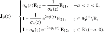
- S-3.:
-
As \(z\rightarrow \infty \),
$$\begin{aligned} \textbf{S}(z)=\textbf{I}+\frac{\textbf{S}_1}{z}+\mathcal {O}(z^{-2}),\qquad \text {with}\quad \textbf{S}_1:=\textbf{T}_1. \end{aligned}$$ - S-4.:
-
The matrix \(\textbf{S}\) remains bounded near the points \(z=-a,0\).

Before moving to the construction of the mentioned parametrices, we conclude this section with the needed estimate for the jump matrix \(\textbf{J}_{\textbf{S}}\) away from \([-a,0]\). For that, recall the matrix norm notation introduced in (6.1), (6.2), (6.3).
Proposition 10.1
For \(U_0\) as in Proposition 8.2, introduce the set
For some \(\varepsilon >0\), and possibly reducing \(U_0\) if necessary, there is an \(\eta >0\) such that
as \(n\rightarrow \infty \).
Proof
From Proposition 8.1-(iv) we obtain that for any \(\varepsilon >0\) there is a constant \(\eta '>0\) for which
On the other hand, the jump conditions on Proposition 8.1-(ii) combined with Cauchy-Riemann equations imply in a standard way that \({{\,\textrm{Re}\,}}\phi \le - \eta \) along the lipses of the lenses and away from the endpoints \(-a\) and 0, as long as the lens stay within a positive but small distance from the interval \([-a,0]\). From these pointwise estimates, the growth of \({{\,\textrm{Re}\,}}\phi \) as \(z\rightarrow \pm \infty \) and the fact that \(\sigma _n\) remains bounded on \(\mathbb {R}\) and \(1/\sigma _n\) grows at most with \(\mathcal {O}({{\,\mathrm{\mathrm e}\,}}^{c n^{2/3}})\) on compacts of \(\mathbb {C}\), the claimed \(L^p\) estimates follow in a standard manner. \(\square \)
10.3 Global parametrix
The global parametrix problem, obtained after neglecting the jumps of \(\textbf{S}\) that are exponentially close to the identity, is the following RHP.
- G-1.:
-
\(\textbf{G}:\mathbb {C}{\setminus } [-a,0] \rightarrow \mathbb {C}^{2\times 2}\) is analytic.
- G-2.:
-
For \(z\in (-a,0)\), it satisfies the jump
$$\begin{aligned} \textbf{G}_+(z)=\textbf{G}_-(z)\left( \sigma _n(z)\textbf{E}_{12}-\frac{1}{\sigma _n(z)}\textbf{E}_{21}\right) . \end{aligned}$$ - G-3.:
-
As \(z\rightarrow \infty \),
$$\begin{aligned} \textbf{G}(z)=\textbf{I}+\mathcal {O}(z^{-1}). \end{aligned}$$ - G-4.:
-
\(\textbf{G}\) has square-integrable singularities at \(z=-a,0\).
The construction of the global parametrix follows standard techniques. First, one introduces a function that we denote \(\mathsf q(z)\), with the aim at transforming the RHP for \(\textbf{G}\) to a RHP with constant jumps. Then, by diagonalizing the resulting jump matrix, we further reduce the problem to two scalar-valued RHPs. With the help of Plemelj’s formula, we then solve these scalar RHPs, and by tracing back all the transformations we recover the matrix \(\textbf{G}\) itself.
The procedure just described is standard in RHP literature, see for instance [7, Appendix A.1], so we refrain from completing it in detail and instead only describe the final form of the solution.
The function \(\sigma _n\) does not vanish and is real and positive over the real axis, so its real logarithm over the real axis is well defined. With this in mind, introduce
where \((\cdot )^{1/2}\) stands for the principal branch of the square root and \(\sqrt{\cdot }\) is reserved for the standard positive real root of positive real numbers. This function \(\mathsf q\) depends on n but we do not make this dependence explicit for ease of notation. It is analytic on \(\mathbb {C}{\setminus } [-a,0]\), and it is chosen to satisfy the jump condition
Furthermore, standard calculations show that
with coefficients given by
Next, set
which is consistent with (4.4), and introduce
This matrix \(\textbf{M}\) satisfies
where \(\varvec{\sigma }_2\) is the second Pauli matrix (recall (3.2)).
Then the solution to the global parametrix RHP- \(\textbf{G}\) is
This solution \(\textbf{G}\) satisfies
Recall that \(U_0\) denotes the neighborhood of the origin given in Proposition 8.2. We will also need some control on \(\mathsf q\) inside \(U_0\).
For the next result, set
which are n-independent quantities. The index \(\beta \) does not have any specific meaning for what comes later, but it arises naturally from the asymptotic analysis resulting in the following result.
Lemma 10.2
For any fixed \(\mathsf s_0>0\), the estimate
is valid uniformly for \(\mathsf s\ge -\mathsf s_0\). In addition, the estimates
are valid uniformly for z on compacts of \(\mathbb {C}{\setminus } [-a,0]\) (in particular on \(\partial U_0\)) and uniformly for \(\mathsf s\ge -\mathsf s_0\), and carry through to boundary values \(\mathsf q_\pm (x)\) for x along \(\mathbb {R}{\setminus } \{-a,0\}\).
Finally,
uniformly for \(z\in \partial U_0\) and \(s\ge -\mathsf s_0\).
Proof
The estimate for \(\mathsf q_0(n)\) follows immediately from an application of Proposition A.2. The estimates for \(\mathsf q(z)\) and \(\mathsf q'(z)\) also follow from Proposition A.2, once we observe that the integrals defining them can be slightly deformed to the upper/lower half plane in a neighborhood of the unique point in the intersection \(\partial U_0\cap (-a,0)\).
Finally, using the first part of the statement and the fact that \(\textbf{M}\) is bounded for \(z\in \partial U_0\) and independent of n, we expand the exponentials in series and write
and the last claim follows after rearranging the terms in this expansion. \(\square \)
10.4 Local parametrix near \(-a\)
The local parametrix \(\textbf{P}=\textbf{P}^{(a)}\) near \(z=-a\) is constructed in a neighborhood of \(z=-a\) which without loss of generality can be taken to be the disk \(D_\delta (-a)\) of radius \(\delta \) around a, and it is the solution to the following RHP.
- \(\textbf{P}^{({a})}\)-1.:
-
The matrix \(\textbf{P}^{(a)}:D_\delta (-a){\setminus } \Gamma _{\textbf{S}}\rightarrow \mathbb {C}^{2\times 2}\) is analytic.
- \(\textbf{P}^{({a})}\)-2.:
-
For \(z\in \Gamma _{\textbf{S}}\cap \partial D_\delta (-a)\), it satisfies the jump \(\textbf{P}^{(a)}_+(z)=\textbf{P}^{(a)}_-(z)\textbf{J}_{\textbf{S}}(z)\).
- \(\textbf{P}^{({a})}\)-3.:
-
Uniformly for \(z\in \partial D_\delta (-a)\),
$$\begin{aligned} \textbf{P}^{(a)}(z)=\left( \textbf{I}+ o (1)\right) \textbf{G}(z),\quad n\rightarrow \infty . \end{aligned}$$ - \(\textbf{P}^{({a})}\)-4.:
-
The matrix \(\textbf{P}^{(a)}\) remains bounded as \(z\rightarrow -a\).
The asymptotic condition \(\textbf{P}^{({a})}\)-3. above will be improved to (10.13) below.
From the conditions on Q, we know that there exists a value \(\eta >0\) for which
This value is uniform for \(\mathsf t\in [\mathsf t_0,1/\mathsf t_0],\) for any \(\mathsf t_0\in (0,1)\) fixed, and it is independent of \(\mathsf s\in \mathbb {R}\). In particular, once we fix \(\mathsf s_0>0\) and assume that \(\mathsf s\ge -\mathsf s_0\), from this inequality we obtain
This way, for \(n>0\) sufficiently large the function \(\sigma _n\) admits an analytic continuation to the whole disk \(D_\delta (-a)\), and this continuation does not have zeros on the same disk. Thus, a branch of \(\log \sigma _n\) is well defined in a neighborhood of \(z=-a\), and the just mentioned estimate also shows that
uniformly for z in a neighborhood of \(z=-a\) and \(\mathsf s\ge -\mathsf s_0\).
With this in mind, the parametrix \(\textbf{P}^{(a)}\) can be constructed explicitly out of Airy functions in a standard way, see for instance [42, Section 7.6]. Since it involves a somewhat nonstandard matching analytic prefactor that accounts for \(\sigma _n\), we briefly go over this construction.
Recall the contour \(\mathsf \Sigma \) introduced in (4.1). With appropriate Airy functions, we construct a \(2\times 2\) matrix \(\varvec{\Psi }_{{{\,\textrm{Ai}\,}}}\), which is analytic on \(\mathbb {C}{\setminus } \mathsf \Sigma \) and satisfies
and
In fact, \(\varvec{\Psi }_{{{\,\textrm{Ai}\,}}}\) can be obtained with a modification of the matrix \({{\varvec{\Phi }}}_\textrm{Ai}\) which we previously used in (6.4). We will not need its explicit form, so we do not write it down explicitly.
Using the properties of \(\phi \) we construct a conformal map \(\varphi \) from a neighborhood of \(-a\) to a neighborhood of the origin, with
With standard arguments (see for instance the proof of Proposition 10.5 below for similar arguments), one shows that the matrix
is analytic on a neighborhood of \(z=-a\). The local parametrix then takes the form
As a result, the error term in fact takes on the stronger form
which is valid uniformly for \(z\in \partial D_\delta (-a)\) and uniformly for \(\mathsf s\ge -\mathsf s_0\) and \(\mathsf t\in [\mathsf t_0,1/\mathsf t_0]\), for any \(\mathsf s_0>0\) and \(\mathsf t_0\in (0,1)\) fixed.
10.5 Local parametrix near the origin
The local parametrix near the origin requires the model problem from Sect. 4.
Recall the neighborhood \(U_0\) of the origin introduced in Proposition 8.2. The initial local parametrix we seek for should be the solution to the following RHP.
- \(\textbf{P}^{(0)}\)-1.:
-
The matrix \(\textbf{P}^{(0)}:U_0{\setminus } \Gamma _{\textbf{S}}\rightarrow \mathbb {C}^{2\times 2}\) is analytic.
- \(\textbf{P}^{(0)}\)-2.:
-
For \(z\in \Gamma _{\textbf{S}}\cap U_0\), it satisfies the jump \(\textbf{P}^{(0)}_+(z)=\textbf{P}^{(0)}_-(z)\textbf{J}_{\textbf{S}}(z)\).
- \(\textbf{P}^{(0)}\)-3.:
-
Uniformly for \(z\in \partial U_0\),
$$\begin{aligned} \textbf{P}^{(0)}(z)=\left( \textbf{I}+ o (1)\right) \textbf{G}(z),\quad n\rightarrow \infty . \end{aligned}$$ - \(\textbf{P}^{(0)}\)-4.:
-
\(\textbf{P}^{(0)}\) remains bounded as \(z\rightarrow 0\).
To construct the solution \(\textbf{P}^{(0)}\) required above, some work is needed. Aiming at removing \(\phi \) from the jump of \(\textbf{P}^{(0)}\), we change this RHP-\(\textbf{P}\) with the transformation
Then the matrix \(\textbf{L}\), should it exist, must satisfy the following RHP.
- \(\textbf{L}\)-1.:
-
The matrix \(\textbf{L}:U_0{\setminus } \Gamma _{\textbf{S}}\rightarrow \mathbb {C}^{2\times 2}\) is analytic.
- \(\textbf{L}\)-2.:
-
For \(z\in \Gamma _{\textbf{S}}\cap U_0\), it satisfies the jump \(\textbf{L}_+(z)=\textbf{L}_-(z)\textbf{J}_{\textbf{L}}(z)\), with
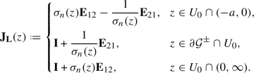 (10.15)
 - \(\textbf{L}\)-3.:
-
Uniformly for \(z\in \partial U_0\),
$$\begin{aligned} \textbf{L}(z)=\left( \textbf{I}+ o (1)\right) \textbf{G}(z){{\,\mathrm{\mathrm e}\,}}^{-n\phi (z)\varvec{\sigma }_3 },\quad n\rightarrow \infty . \end{aligned}$$ - \(\textbf{L}\)-4.:
-
The matrix \(\textbf{L}\) remains bounded as \(z\rightarrow 0\).

Based on the usual way of matching the local parametrix with a model problem, one is tempted to moving the non-constant part of the jump - namely \(\sigma _n\) - to the behavior at \(\partial U_0\) as well. This would be done so including a term of the form \(\sigma _n^{\varvec{\sigma }_3/2}={{\,\mathrm{\mathrm e}\,}}^{\varvec{\sigma }_3\log \sigma _n/2}\) into the transformation \(\textbf{P}\mapsto \textbf{L}\), in much the same way we did in (10.12). However, as we discussed in Sect. 3.1, for any \(s\in \mathbb {R}\) fixed there are poles of \(\sigma _n\) accumulating too fast near the origin, so \(\sigma _n\) fails to be analytic in any small neighborhood of the origin and we have to stick to the non-constant jumps as above.
The RHP-\(\textbf{L}\) has a solution if, and only if, RHP-\(\textbf{P}^{(0)}\) has a solution. Such solutions need not be unique, as one could possibly improve on the asymptotic matching conditions on \(\partial U_0\). The goal of the rest of this section is to describe a solution \(\textbf{L}\), and consequently a solution \(\textbf{P}^{(0)}\) related by (10.14), with a more explicit control of the error term in RHP-\(\textbf{L}\)-3. For that, we use the model problem thoroughly studied in Sects. 4 and 7.
The construction that follows needs several quantities that appeared before. These are the conformal map \(\psi \) appearing in Proposition 8.2, the function \(\mathsf H_Q\) introduced with the help of Proposition 8.3, the model RHP solution \({\varvec{\Phi }}={\varvec{\Phi }}(\cdot \mid \mathsf h)\) introduced in Sect. 4 and further discussed in Sect. 7, and the constant \(\mathsf q_0\) and matrices \(\textbf{U}_0\) and \(\textbf{M}(z)\) from (10.3)–(10.5). With all these quantities at hand, we set
With the identification \(\tau =n^{2/3}\) and thanks to Proposition 8.3, the function \(\mathsf h_n\) becomes admissible in the sense of Definition 4.1, so the notation for the corresponding solution \({\varvec{\Phi }}_n={\varvec{\Phi }}(\cdot \mid \mathsf h_n)\) chosen above is consistent with the solution \({\varvec{\Phi }}_\tau (\zeta )\big |_{\tau =n^{2/3}}\) in (4.5). For later reference, we keep track of the expansion
compare (8.7) with Definition 4.1-(ii).
Proposition 10.3
Fix \(\mathsf s_0>0\) and \(\mathsf t_0\in (0,1)\). There exists \(n_0=n_0(\mathsf s_0,\mathsf t_0)\) for which for any \(s\ge -\mathsf s_0\) and any \(\mathsf t\in [\mathsf t_0,1/\mathsf t_0]\) the matrix \({{\varvec{\Phi }}}_n\) exists for every \(n\ge n_0\). This matrix satisfies the jump
Furthermore, for the matrix
the asymptotic expansion
holds true uniformly for \(z\in \partial U_0\) and uniformly for \(\mathsf s\ge -\mathsf s_0\) and \(\mathsf t\in [\mathsf t_0,1/\mathsf t_0]\).
Proof
The existence of \({{\varvec{\Phi }}}_n\) is granted by the first claim of Theorem 7.1. The jumps for \({{\varvec{\Phi }}}_{n,+}\) follow from the jumps in (4.2), the definition of \(\mathsf h_n\) taken in (10.16), the correspondence (8.6) and the conformality of the change of variables \(\zeta =n^{2/3}\psi (z)\). The asymptotic expansion for \({{\varvec{\Phi }}}_n\) is immediate from (4.3) \(\square \)
The introduction of the additional notation \(\widehat{{\varvec{\Phi }}}_n\), which plays the role of the local parametrix in the variable \(\zeta \), is convenient for later calculations. At that moment, some of its properties will be needed, and we keep track of these properties with the next result. For the formal statement, we recall that \(\Phi (\xi \mid \mathsf S,\mathsf T)\) is the solution to the integro-differential PII that already appeared in (2.11) and (5.15), and \({\varvec{\Phi }}_0^{(1)}\) is the residue matrix from (5.17) that collects the functions \(\mathsf P(\mathsf S,\mathsf T)\) and \(\mathsf Q(\mathsf S,\mathsf T)\) which, in turn, are related to \(\Phi \) as explained in (5.13) et seq..
Proposition 10.4
Fix \(\mathsf s_0>0\) and \(\mathsf t_0\in (0,1)\) and \(\nu \in (0,2/3)\), and let \(\mathsf c_{\mathsf H}\) be as in (8.7). The following asymptotic formulas hold true uniformly for \(\mathsf s\ge -\mathsf s_0\) and \(\mathsf t\in [\mathsf t_0,1/\mathsf t_0]\).
The matrix \({\varvec{\Phi }}_n^{(1)}\) from Proposition 10.3 satisfies
Furthermore, for \({{\varvec{\Phi }}}_0\) being the solution to the RHP in (5.9)–(5.10), the estimate
holds true uniformly for \(\zeta \in \mathsf \Sigma \) with \(|\zeta |\le n^{\frac{1}{3}-\frac{1}{2}\nu }\).
Proof
It is immediate from the identification \(\tau =n^{2/3}\), Eq. (10.16) and Theorem 7.1. \(\square \)
Next, we now verify that \(\textbf{L}\) given as in (10.16) indeed solves the RHP-\(\textbf{L}\).
Proposition 10.5
The matrix \(\textbf{L}\) solves the RHP-\(\textbf{L}\).
Furthermore, setting
the condition \(\textbf{L}\)-3. is improved to
uniformly for \(z\in \partial U_0\) and \(\mathsf s\ge -\mathsf s_0\), \(\mathsf t\in [\mathsf t_0,1/\mathsf t_0]\), for any \(\mathsf s_0>0,\mathsf t_0\in (0,1)\).
Proof
First we prove that \({\textbf{F}}\) is analytic. For that, notice that a jump for it may come only from the factors \(\textbf{M}\) and \(\psi ^{1/4}\), and therefore only possibly in the interval \((-a,0)\cap U_0\). However, along this interval it is simple to compute that \((\psi ^{1/4})_\pm = {{\,\mathrm{\mathrm e}\,}}^{\pm \pi \textrm{i}/4}|\psi |^{1/4}\), and also that
from which we obtain
so \({\textbf{F}}\) is indeed analytic across \((-a,0)\cap U_0\). In principle, \({\textbf{F}}\) may have an isolated singularity at 0, but because
we see that \(z=0\) is a removable singularity. In virtue of the definition of \(\textbf{L}\) in (10.16) and the jump for \({\varvec{\Phi }}_n\) from Proposition 10.3, the analyticity of \(\textbf{F}\) is enough to conclude that \(\textbf{L}\) satisfies RHP.\(\textbf{L}\)-1.
Knowing that \({\textbf{F}}\) is analytic, the jump for \(\textbf{L}\) is precisely the same as the jump for \({{\varvec{\Phi }}}_n\), and by Proposition 10.3 we thus have that \(\textbf{L}\) satisfies RHP.\(\textbf{L}\)-2.
Finally, to the asymptotic condition (10.20). For that, we use the asymptotic condition for \({{\varvec{\Phi }}}_n\) given by Proposition 10.3 and the definition of \({\textbf{F}}\) and write
and where the error is uniform for \(z\in \partial U_0\) and \(\mathsf s,\mathsf t\) as claimed. Since \(\partial U_0\) remains within a positive distance from the unique zero \(z=0\) of \(\psi \), the function \(|\psi ^{1/4}|\) remains bounded from below away from zero, so the corresponding conjugation of the error by the term \(\psi ^{\varvec{\sigma }_3/4}\) does not change the order of the error. Next, the conjugation by \(n^{\varvec{\sigma }_3/6}\) contributes at most to an error of order \(n^{1/3}\), and only in the (2, 1)-entry. The remaining term \(\textbf{M}\) is bounded along \(\partial U_0\), so it can be commuted with the error term above without changing its order, leading to (10.21). And (10.21) is indeed an improvement of the asymptotic condition RHP.\(\textbf{L}\)-3, because from Lemma 10.2 we know that \(\textbf{M}=(\textbf{I}+\mathcal {O}(n^{-1/3}))\textbf{G}\) uniformly as claimed. \(\square \)
We now trace back the transformation \(\textbf{L}\mapsto \textbf{P}^{(0)}\) and construct the latter as
keeping track that \({{\varvec{\Phi }}}_n\) and \(\textbf{F}_n\) are introduced in (10.16). With this construction and thanks to Lemma 10.2 and (10.21), the matching condition RHP.\(\textbf{P}^{(0)}\)-3 is
and the errors are uniform for \(\mathsf s\ge -\mathsf s_0\) and \(\mathsf t_0\le \mathsf t\le 1/\mathsf t_0\).
10.6 Final transformation
The final transformation combines the local and global parametrices to remove the non-decaying jumps from \(\textbf{S}\).
Set
orienting \(\partial U_0\) and \(\partial D_\delta (-a)\) in the clockwise direction. With \(\textbf{P}^{(a)}\) being the local parametrix near \(-a\), \(\textbf{P}^{(0)}\) the local parametrix near the origin and \(\textbf{G}\) the global parametrix, we introduce a last parametrix \(\textbf{P}\) with unified notation as
The final transformation \(\textbf{S}\mapsto \textbf{R}\) is then
With this transformation, the jumps that \(\textbf{S}\) has in common with the parametrices \(\textbf{G}\) and \(\textbf{P}\) get canceled, and we remain with jumps only away from \([-a,0]\) and U. With
the matrix \(\textbf{R}\) satisfies the following RHP.
- R-1.:
-
The matrix \(\textbf{R}:\mathbb {C}{\setminus } \Gamma _{\textbf{R}}\rightarrow \mathbb {C}^{2\times 2}\) is analytic.
- R-2.:
-
For \(z\in \Gamma _{\textbf{R}}\), it satisfies the jump \(\textbf{R}_+(z)=\textbf{R}_-(z)\textbf{J}_{\textbf{R}}(z)\), with
 (10.24)
 - R-3.:
-
With \(\textbf{R}_1:=\textbf{S}_1-\textbf{G}_1\),
$$\begin{aligned} \textbf{R}(z)=\textbf{I}+\frac{1}{z}\textbf{R}_1+\mathcal {O}(1/z^2),\quad z\rightarrow \infty . \end{aligned}$$(10.25)

To conclude that \(\textbf{R}\) is asymptotically close to the identity, we control its jumps. We use the matrix norm notation introduced in (6.1)–(6.3).
Proposition 10.6
Fix \(\mathsf s_0>0\) and \(\mathsf t_0\in (0,1)\). There is \(\eta >0\) for which the jump matrix for \(\textbf{R}\) satisfies the estimates
and
as \(n\rightarrow \infty \), uniformly for \(\mathsf s\ge -\mathsf s_0\) and \(\mathsf t_0\le \mathsf t\le 1/\mathsf t_0\).
Proof
The function \(\textbf{G}\) remains uniformly bounded away from the interval \([-a,0]\), and the first claimed decay then follows from (10.24) and Proposition 10.1.
Using (10.13) and (10.24), we obtain the uniform estimate of the jump along \(\partial D_\delta (-a)\) directly. Since \(\partial D_\delta (-a)\) is bounded, the \(L^1\) and \(L^2\) estimates also follow. Finally, estimate for the jump along \(\partial U_0\) follows similarly, once we recall (10.23). \(\square \)
With Proposition 10.6 at hand, the small norm theory of Riemann–Hilbert problems yields
Theorem 10.7
Fix \(\mathsf s_0>0\) and \(\mathsf t_0>0\). The matrix \(\textbf{R}\) satisfies
and the residue matrix \(\textbf{R}_1\) satisfies
where the error terms are all uniform for z, w on the same connected components of \(\mathbb {C}{\setminus } \Gamma _{\textbf{R}}\), and they are also uniform for \(\mathsf s\ge -\mathsf s_0\) and \(\mathsf t_0\le \mathsf t\le 1/\mathsf t_0\).
Proof
The arguments are standard, so we only sketch them. The small norm theory for RHPs ensures the representation
This ensures the estimates for \(\textbf{R}\) and \(\textbf{R}'\) away from \(\Gamma _{\textbf{R}}\) and, because the jump matrix is analytic on a neighborhood of \(\Gamma _{\textbf{R}}\), we are able to extend these estimates also to \(\Gamma _{\textbf{R}}\). To obtain the estimate involving z and w, we then write, with the help of Cauchy’s formula,
where the integral is over a contour on \(\textbf{C}{\setminus } \Gamma _{\textbf{R}}\) encircling both w and z. The right-hand side is now \(\textbf{I}+\mathcal {O}((w-z)n^{-1/3})\) by the estimate on \(\textbf{R}\) already proven.
Finally, the estimate for \(\textbf{R}_1\) follows expanding (10.27) as \(z\rightarrow \infty \), and then using that the jump matrix decays to the identity at least as \(\mathcal {O}(n^{-1})\) away from \(\partial U_0\). \(\square \)
Later on, we also need the first term in the asymptotic expansion for \(\textbf{R}\), we state it as a separate result.
Proposition 10.8
Fix \(\mathsf s_0>0\) and \(\mathsf t_0>0\). Setting
the matrix \(\textbf{R}\) has the expansion
where the error term is uniform for \(z\in U_0\), and it is also uniform for \(\mathsf s\ge -\mathsf s_0\) and \(\mathsf t_0\le \mathsf t\le 1/\mathsf t_0\).
Proof
Starting from the representation (10.27), we write
and the result follows combining (10.24) and (10.23) and performing straightforward calculations. \(\square \)
All the transformations \(\textbf{Y}\mapsto \textbf{T}\mapsto \textbf{S}\mapsto \textbf{R}\) involve only analytic factors in their construction. As such, we can actually slightly deform the contour \(\Gamma _{\textbf{R}}\) in all these steps, so that in fact the estimates in the previous result are valid everywhere on \(\mathbb {C}\), interpreting them as with boundary values when \(z,w\in \Gamma _{\textbf{R}}\). We will use this fact without further warning.
With this theorem at hand, in the next sections we recover the needed asymptotic formulas for the proof of our main results.
11 Proof of Main Results
The next step in the direction of concluding our asymptotic analysis is to unravel the transformations \(\textbf{R}\mapsto \textbf{S}\mapsto \textbf{T}\mapsto \textbf{Y}\). Introduce
which are related by
Then the result of the unfolding of the transformations is
We split the proofs of our results in the next few sections.
11.1 Proof of Theorem 2.4
Thanks to (11.1) and Theorem 10.7, the expression (9.10) reduces to the asymptotic formula
valid as \(n\rightarrow \infty \), \(x,y\in \mathbb {R}\) and uniformly for \(\mathsf s,\mathsf t\) as in Theorem 10.7.
For the value \(\mathsf c_V>0\) introduced in (8.5), we scale \(x=u_n\) and \(y=v_n\) as in (2.18), where u, v are on any given compact of the real axis. For such values of u, for n large enough the points \(u_n\) are always on the neighborhood \(U_0\) of the origin where \(\textbf{P}=\textbf{P}^{(0)}\), and from (10.22) we simplify
where all the quantities above are evaluated at \(u_n\). The next step is to plug these identities into (11.2), when doing so we also use the estimates
which follows from (10.16), (10.4) and (8.5), and its immediate consequence
which is obtained with arguments similar to (10.28). These estimates are uniform for u, v in compacts of \(\mathbb {R}\), and are also uniform for \(\mathsf s\ge -\mathsf s_0\) and \(\mathsf t\in [\mathsf t_0,1/\mathsf t_0]\). Equation (11.2) then simplifies to
Now, with the definition of \({\varvec{\Phi }}_n\) in (10.16) at hand, the aid of (10.19) and the constant \(\mathsf c_{\mathsf H}\) appearing in (10.17), we get
for any \(\nu \in (0,2/3)\), with the error being valid uniformly for u in compacts of \(\mathbb {R}\), and also uniformly for \(\mathsf s\ge -\mathsf s_0, \mathsf t_0\le \mathsf t\le 1/\mathsf t_0\). Also, thanks to Theorem 5.1 we know that \({{\varvec{\Phi }}}_{0,+}(u\mid \mathsf s,\mathsf c_{\mathsf H})^{\pm 1}\) remain bounded for u in compacts and \(\mathsf s\ge -\mathsf s_0, \mathsf t_0\le \mathsf t\le 1/\mathsf t_0\). Therefore,
as \(n\rightarrow \infty \). In addition, the estimate
is valid uniformly for u in compacts, uniformly for \(\mathsf s\in \mathbb {R}\) and \(\mathsf t_0\le \mathsf t\le 1/\mathsf t_0\), and is immediate from (2.16). Combining everything, and denoting \(\chi _+=\chi _{[0,\infty )}\), we obtained the asymptotic formula
which is valid uniformly for u, v in compacts of \(\mathbb {R}\), and also uniformly for \(\mathsf s\ge -\mathsf s_0\) and \(\mathsf t_0\le \mathsf t\le 1/\mathsf t_0\). With \({{\varvec{\Delta }}}_0\) as in (5.7), this identity rewrites as
and the proof of Theorem 2.4 is now completed using Eq. (5.16).
11.2 Proof of Theorem 2.5
Now that the RHP asymptotic analysis is completed, the proof of Theorem 2.5 follows standard steps. In our case, there is an additional cancellation that has to be accounted for at a later step, in virtue of the presence of the factor \(\mathsf q\) in both the global and local parametrices, see (10.6) and (10.23). So we opt for presenting the detailed calculation.
Starting from the representation (9.8), we unravel the transformations and obtain
with \(\textbf{R}_1\) as in (10.25), and where for the second identity we used the definition of \(\textbf{G}_1\) in (10.7) and the estimate for \(\mathsf q_0\) from Lemma 10.2.
It remains to estimate \(\textbf{R}_1\), which we do so starting from (10.26). Using Cauchy-Schwartz, Propositions 10.6 and Theorem 10.7, we write
The matrix \(\textbf{J}_\textbf{R}\) is in (10.24), and combining its explicit expression along \(\partial U_0\) with (10.23) and (10.5), after a cumbersome but straightforward calculation we arrive at
where we recall that \(\mathsf m\), \(\mathsf q^{(1)}\) and \(\textbf{L}_1\) are given in (10.4), (10.8) and (10.20), respectively. Using this explicit expression for \(\textbf{L}_1\), we see that
Both functions \(\mathsf m\) and \(\psi \) are analytic in a neighborhood of the origin, and vanish linearly therein. Combining in addition with (8.5), we see that the product \(\mathsf m(z)^{1/2}\psi (z)^{1/2}\) admits an analytic continuation near the origin, with the expansion
Thus, computing residues
Similarly, using now (10.8) we obtain
Hence,
and (11.4) updates to
uniformly for \(\mathsf s\ge -\mathsf s_0\) and \(\mathsf t_0\le \mathsf t\le 1/\mathsf t_0\). We now need only to apply (10.18) with any \(\nu \ge 1/3\) to complete the proof.
11.3 Proof of Theorem 2.2
Unlike the already proven major results, the proof of Theorem 2.2 is not a straightforward consequence of the steepest descent analysis concluded with Theorem 10.7. It does rely substantially on Theorem 10.7, but several other inputs are also needed along the way. Equipped with (9.10), the idea is to account for the different approximations for \(\mathsf K_n^Q\) on the different components
that arise from the RHP, and integrate each such approximation. With Proposition 9.1 in mind, we are thus able to recover asymptotics for \(\mathsf L_n^Q\) itself. As one would expect, it turns out that in this process the terms that arise away from \(U_0\) become all exponentially negligible, and only the contribution from \(U_0\) survives in the leading contribution. The contribution that arrives this way involves \({\varvec{\Phi }}_n\), and we further need to split it into different parts and still account for some exact cancellations to arrive at the leading asymptotic contribution. We postpone this analysis to the next section, where it is split into several different lemmas, and summarize the outcome with the next result. For its statement, we recall that \(\mathsf h_n\) and \(\widehat{{\varvec{\Phi }}}_n\) were introduced in (10.16), and we also set
Proposition 11.1
Fix \(\mathsf s_0>0\) and \(\mathsf t_0\in (0,1)\). There exists a function \(\mathsf R(u)=\mathsf R_1(u\mid \mathsf t)\) satisfying
uniformly for \(\mathsf s\ge -\mathsf s_0\) and \(\mathsf t_0\le \mathsf t\le 1/\mathsf t_0\), and for which the identity
holds true for every \(u\ge -\mathsf s_0\) and every \(\mathsf t\in [\mathsf t_0,1/\mathsf t_0]\).
In words, Proposition 11.1 is saying that the major contribution to \(\mathsf L_n^Q\) comes from the neighborhood \(U_0\), so from the local parametrix \(\widehat{{\varvec{\Phi }}}_n\). But according to the developments from the previous sections, this local parametrix is close to the id-PII parametrix \({{\varvec{\Phi }}}_0\), and we are ready to conclude our last major result.
Proof of Theorem 2.2
We combine Propositions 9.1 and (11.1) to obtain
valid as \(n\rightarrow \infty \) and uniformly for \(\mathsf s\ge -\mathsf s_0\) and \(\mathsf t_0\le \mathsf t\le 1/\mathsf t_0\). Next, with the identifications (10.16)–(10.17) in mind, we estimate the integral on the right-hand side with the help of Theorem 7.2 and conclude the proof. \(\square \)
12 Technical Lemmas
It remains to prove Proposition 11.1, analysis which we split into several technical lemmas in this section.
Our starting point is the integral representation for \(\mathsf L_n^Q\) from Proposition 9.1 with the asymptotic information for \(\mathsf K_n^Q\) provided by the RHP analysis. For \(x\in \mathbb {R}\), set
Recalling (9.11), the unwrap of the transformations of the RHP yields the identity
We now need to integrate each of the terms on the right-hand side above, first in \(x\in \mathbb {R}\) and then in \(u\in (\mathsf s,+\infty )\). Each term will be analyzed individually, also depending on whether we integrate x in the bulk, each of the edges or away from the support \([-a,0]\) of the equilibrium measure. To simplify notation, it is convenient to introduce the additional notation for each relevant integral, and for an arbitrary set \(J\subset \mathbb {R}\) denote
and
which are functions of \(u\in \mathbb {R}\) as well. With \(\varepsilon _0,\varepsilon _1>0\) being determined by \((-\varepsilon _0,\varepsilon _1)=U_0\cap \mathbb {R}\), the split
is immediate, and with the next series of lemmas we estimate each of the terms on the right-hand side.
Lemma 12.1
Fix \(\mathsf s\in \mathbb {R}\) and \(\mathsf t_0\in (0,1)\). There exists \(\eta >0\) for which the estimate
holds true uniformly for \(u\ge \mathsf s\) and \(\mathsf t_0\le \mathsf t\le 1/\mathsf t_0\).
Proof
On the intervals \((-\infty ,-a-\delta )\) and \((\varepsilon _1,\infty )\) the function \(\varvec{\Lambda }_{n}\) is identically the identity matrix. On the interval \((a+\delta ,-\varepsilon _0)\) the nontrivial entry of \(\varvec{\Lambda }_{n}\) is \({{\,\mathrm{\mathrm e}\,}}^{2n\phi _+}/\sigma _n\) and, because \(Q<0\) and \(\phi _{+}\) is purely imaginary in this interval, this quotient is bounded. Also, away from the endpoints \(-a\) and 0 we have \(\textbf{P}\equiv \textbf{G}\). Both \(\textbf{P}\) and \(\textbf{G}\), and their x-derivatives, decay as \(x\rightarrow \pm \infty \) and remain bounded as \(n\rightarrow \infty \), all uniformly in u and \(\mathsf t\) as claimed. All of these facts combined together, we obtain that for some constants \(K>0\) and \(n_0\ge 1\)
Next, we now use that \(Q\ge 0\) on the interval \((-\infty ,0)\) to bound
which is valid for any \(n\ge 1, u\in \mathbb {R},\mathsf t>0\). Thus, combining everything we obtain
and using Proposition 8.1-(iv), (v), this proves the bound for \(\mathsf I_1(-\infty ,-a-\delta )\).
For the second integral, we term \(\phi _+\) is oscillatory, so to obtain the exponential decay in the x-integral we have to argue differently and as follows. The function
is strictly increasing on \((-\infty ,0)\) and strictly decreasing on \((0,+\infty )\). Because \(Q>0\) on \((-\infty ,0)\) and \(Q(0)=0\), by reducing \(U_0\) if necessary we can assume without loss of generality that \(Q(x)\ge Q(-\varepsilon _0)\) for every \(x\in [-a,-\varepsilon _0]\). This way, \(v=u+n^{2/3}Q(x)\ge v_0:=u+n^{2/3}Q(-\varepsilon _0)\) and, because u is assumed to be bounded from below, we can make sure that \(v_0>0\) for every u. Therefore
and upon integration and using Proposition 8.1-(ii), we obtain
for every \(n\ge n_0\) and \(\mathsf t,u\) as claimed.
For the estimate for \(\mathsf I_2(-a,-\varepsilon _0)\) we use again the last inequality in (12.6) and also that both \(\phi '_{+}\) and \(Q'\) are continuous, and hence bounded, on \((-a,-\varepsilon _0)\). This concludes the proof. \(\square \)
For the integral over \((\varepsilon _1,+\infty )\), it is easier to actually estimate its u-integral directly.
Lemma 12.2
Fix \(\mathsf s_0>0\) and \(\mathsf t_0\in (0,1)\). There exists \(\eta >0\) for which the estimate
holds true uniformly for \(\mathsf s\ge -\mathsf s_0\) and \(\mathsf t_0\le \mathsf t\le 1/\mathsf t_0\).
Proof
With the bound (12.5) we see that it is enough to estimate the integral
where for the equality we used Tonelli’s Theorem to interchange the order of integration, and then integrated exactly. The term \((1+{{\,\mathrm{\mathrm e}\,}}^{\mathsf s+n^{2/3}Q(x)})^{-1}\) is bounded by 1, and using Proposition 8.1-(iv), (v) we see that the integral of \({{\,\mathrm{\mathrm e}\,}}^{-2n\phi }\) is \(\mathcal {O}({{\,\mathrm{\mathrm e}\,}}^{-\eta n})\) for some \(\eta >0\) independent of \(\mathsf s\) and \(\mathsf t\), which concludes the proof. \(\square \)
Next, we analyze the contribution coming from a neighborhood of the endpoint \(z=a\).
Lemma 12.3
Fix \(\mathsf s\in \mathbb {R}\), \(\mathsf t_0\in (0,1)\). There exists \(\eta >0\) such that the estimate
is valid uniformly for \(u\ge \mathsf s\) and \(\mathsf t_0\le \mathsf t\le 1/\mathsf t_0\).
Proof
On the neighborhood \(D_\delta (-a)\) the function \(\textbf{P}=\textbf{P}^{(a)}\) is the Airy local parametrix (10.12), which involves the function \({\varvec{\Phi }}_{{{\,\textrm{Ai}\,}}}\) evaluated at the argument \(\zeta =n^{2/3}\varphi (z)\). In the \(\zeta \)-plane, we fix \(R>0\) for which the asymptotic expansion (10.10) is valid for \(|\zeta |>R\), and split the analysis into two cases, namely for \(|n^{2/3}\varphi (z)|\le R\) and \(|n^{2/3}\varphi (z)|\ge R\), and for
we write
and now analyze each integral on the right-hand side separately.
For \(|n^{2/3}\varphi (z)|\le R\), the terms \({\varvec{\Phi }}_{{{\,\textrm{Ai}\,}},+}(\zeta =n^{2/3}\varphi (z))\) and \({\varvec{\Phi }}'_{{{\,\textrm{Ai}\,}},+}(\zeta =n^{2/3}\varphi (z))\) consist of continuous functions evaluated inside the compact interval \([-R,R]\), and therefore they are bounded. By the same reason, the expression (10.11) shows that \(\textbf{F}\) is bounded for \(|n^{2/3}\varphi (z)|\le R\). On the other hand, without further analysis we obtain that \(\textbf{F}'\) may grow at most as \(\mathcal {O}(n^{1/6})\). Finally, combining with (10.9) and the fact that the determinant of \(\textbf{P}\) is identically 1, we conclude that for \(|n^{2/3}\varphi (x)|\le R\),
which is valid as \(n\rightarrow \infty \) and uniformly for \(x\in (-a-\delta ,-a+\delta )\), also uniformly for \(u\ge \mathsf s\) and \(\mathsf t_0\le \mathsf t\le 1/\mathsf t_0\).
We use (12.7) back into (12.1), and combined with the fact that \(|\sigma _n^{-1}|\le 2\) for \(x\le (-\infty ,0)\) the result is that
where the last error term is a scalar error, valid uniformly in \(x,u,\mathsf t\) as before. Integrating, we obtain that for some absolute constant \(K>0\),
where for the second inequality we used that \(0<\sigma _n\le 1\) and for the last estimate we used that Q is strictly positive on \((-a-\delta ,-a+\delta )\supset A_n\).
Next, we consider the case \(|n^{2/3}\varphi (z)|\ge R\). In such situation, the asymptotics (10.10) take place, and when combined with (10.11) they yield
where for the last equality we used (10.9).
The matrix \(\textbf{P}_+\) is bounded as \(x\rightarrow 0\), whereas \(\textbf{G}\) is not, but the cancellation that leads to this boundedness of \(\textbf{P}\) is not captured by this asymptotics. Nevertheless, as we need some uniform control over x, we now account for the behavior of \(x\rightarrow 0\) in a rough manner as follows. We are assuming that \(|n^{2/3}\varphi (x)|\ge R\), and because \(\varphi \) is conformal with \(\varphi (0)=0\) this means that \(|x+a|\ge c/n^{2/3}\), for some fixed \(c>0\). The function \(\textbf{G}\) has a fourth-root singularity at \(x=0\), and therefore we arrive at the rough estimate
The estimate (12.9) can be differentiated term by term. With arguments similar to the ones we just applied, we arrive at the rough estimate
These latter two estimates are valid uniformly for \(u\ge \mathsf s\) and \(\mathsf t_0\le \mathsf t\le 1/\mathsf t_0\) as \(n\rightarrow \infty \).
Finally, on the interval \((-a,0)\) the factor \(\phi _+\) is purely imaginary, implying that \(\varvec{\Lambda }_{n}^{\pm 1}\) remains bounded therein. All combined, we obtained that
uniformly for \(x\in B_n\) and \(u,\mathsf t\) as claimed. Proceeding as in (12.8) we obtain a bound for \(I_1(B_n)\) and complete the proof. \(\square \)
It remains to analyze the two integrals \(\mathsf I_1(-\varepsilon _0,\varepsilon _1)\) and \(\mathsf I_2(-\varepsilon _0,0)\). The hardest analysis is the integral \(\mathsf I_1\) which, as will turn out, contains both the leading contribution, a term to cancel \(\mathsf I_2\) and asymptotically negligible terms. For ease of presentation, we explore the expression for \(\mathsf A\) in (12.1) as a sum and split
where, for any measurable set \(J\subset \mathbb {R}\),
and analyze each of these terms separately. For the estimation of \(\mathsf J_1\), it is also easier to perform the u-integral, just as we did in Lemma 12.2.
Lemma 12.4
Fix \(\mathsf s_0>0\) and \(\mathsf t_0\in (0,1)\). The estimate
holds true uniformly for \(\mathsf s\ge -\mathsf s_0\) and \(\mathsf t_0\le \mathsf t\le 1/\mathsf t_0\).
Proof
The idea is similar to the proof of Lemma 12.3. We fix a number \(R>0\) for which the asymptotic expansion (4.3) for \({\varvec{\Phi }}=\widehat{{\varvec{\Phi }}}_n\) is valid for \(|\zeta |\ge R\), uniformly in \(\mathsf t,\mathsf s\) as claimed (see Remark 7.8). Then, introduce
We now find bounds for the integrands, with separate arguments for each of \(C_n\) and \(D_n\).
Recalling (10.22), on the interval \((-\varepsilon _0,\varepsilon _1)\) the parametrix is \(\textbf{P}=\textbf{P}^{(0)}=\textbf{F}_n{\varvec{\Phi }}_n{{\,\mathrm{\mathrm e}\,}}^{n\phi \varvec{\sigma }_3}\), with \(\textbf{F}_n\) and \({\varvec{\Phi }}_n\) as in (10.16). Using the definition of \(\textbf{F}_n\) in (10.16) and Theorem 10.7, we express
valid uniformly when evaluated at \(x\in C_n\) and also uniformly for \(\mathsf s,\mathsf t\) as claimed. Using again the definition of \(\textbf{F}_n\), the fact that \(\psi /\mathsf m\) remains bounded near \(z=0\) and (10.30),
A careful inspection on (10.29) shows that \((\widehat{\textbf{R}}_1(z))_{12}\) is independent of z, so \(R'\) has zero (1, 2)-entry. Therefore we conclude that
stressing that this is valid for \(x\in C_n\). Also, from (10.19) we learn that \({\varvec{\Phi }}_n(x)=\mathcal {O}(1)\) uniformly on \(C_n\). Everything we have so far combined yields that
Along \((-a,0)\) we have \(Q>0\) so that \(1/\sigma _n\) remains bounded uniformly, and consequently \({\varvec{\Delta }}_{n}=\mathcal {O}(1)\) in the same interval. Using this information in the last displayed equation, we thus obtain that
uniformly for \(u\ge \mathsf s\) and \(\mathsf t_0\le \mathsf t\le 1/\mathsf t_0\), and where the error term is uniform for \(x\in C_n\).
Next, along \(D_n\) we now use the asymptotic expansion (4.3) for \({\varvec{\Phi }}=\widehat{{\varvec{\Phi }}}_n\) and the definition of \(\mathsf F_n\) and obtain that
and similarly
all valid as \(n\rightarrow \infty \), uniformly for \(x\in D_n\) and uniformly in \(u,\mathsf t\) as claimed
With the same arguments that we applied in (12.16), we obtain along \(D_n\) as well
The factor \(\phi _+\) is purely imaginary on \((-a,0)\) and positive on \([0,+\infty )\), so the term \({{\,\mathrm{\mathrm e}\,}}^{-2n\phi _+}\) in the integrand above is bounded by a uniform constant. Combining with (12.17), we conclude
Finally, we now integrate in u and use Tonelli’s Theorem to interchange the order of integration, obtaining just like in the proof of Lemma 12.2 that
which concludes the proof. \(\square \)
Next, in our pursuit of analyzing (12.4), the final missing piece of the puzzle is the term \(\mathsf J_2(-\varepsilon _0,\varepsilon _0)\) that arises from \(\mathsf I_1(-\varepsilon _0,\varepsilon _0)\). To state the rigorous results, we recall once again that the conformal map \(\psi \) was introduced in Proposition 8.2, the function \(\mathsf h_n\) is given in (10.16), the function \(\widehat{{\varvec{\Delta }}}_n\) is in (11.5) and in addition also set
Lemma 12.5
Fix \(\mathsf s_0>0\) and \(\mathsf t_0\in (0,1)\). There exists a function \(\mathsf R_1(u)=\mathsf R_n(u\mid \mathsf t)\) satisfying the estimate
uniformly for \(\mathsf s\ge -\mathsf s_0\) and \(\mathsf t_0\le \mathsf t\le 1/\mathsf t_0\), and for which the identity
holds true for every \(u\in \mathbb {R}\) and every \(\mathsf t>0\).
Proof
Recall that \(\mathsf J_2\) was introduced in (12.13). In the interval \((-\varepsilon _0,\varepsilon _1)\) the local parametrix \(\textbf{P}=\textbf{P}^{(0)}\) coincides with (10.22). A direct calculation from (10.16) shows that the matrix \(\textbf{F}_n\) therein satisfies the identity
With the help of this identity, we express
where both sides are evaluated at \(x\in (-\varepsilon _0,\varepsilon _1)\). Thus,
We now multiply this last expression by \({{\,\mathrm{\mathrm e}\,}}^{-2n\phi _+}\sigma _n/(1+{{\,\mathrm{\mathrm e}\,}}^{u+n^{2/3}Q})\) and integrate. A direct calculation gives
which is the integrand of \(\mathsf I_2(-\varepsilon _0,\varepsilon _1)=\mathsf I_2(-\varepsilon _0,0)\), see (12.3). Thus, from (12.19) we obtain
where we have set
It is worth mentioning that both \(\mathsf m\) and \(\psi \) have a simple zero at \(x=0\), so the first term in the integrand of \(\mathsf R\) remains bounded near \(x=0\).
Recalling (10.16), the integrand written explicitly in (12.20) is of the form
with obvious choices of the functions \(f_1,\textbf{f}_2,\textbf{f}_3\), and performing the change of variables \(u=n^{2/3}\psi (x)\) we obtain the integral in the right-hand side of (12.18).
To conclude, it remains to show the bound for \(\mathsf R\). For that, we use again the sets \(C_n\) and \(D_n\) from (12.15) and analyze the integral over each of these sets separately.
Along \(C_n\), the convergence (10.19) ensures \({\varvec{\Phi }}_{n,+}\) remains bounded uniformly, and combined with the boundedness of all the other terms on the whole interval \((-\varepsilon _0,\varepsilon _1)\) we obtain
The function \(\psi \) is conformal, and consequently \(|z|\le cn^{-2/3}\) for \(z\in C_n\) and some constant c independent of \(\mathsf t,u,n\). In particular, this ensures that \(n^{2/3}Q(x)\le -\tilde{c}\) for every \(x\in C_n\) and a constant \(\tilde{c}>0\), and therefore
Still because \(\psi \) is conformal, we are sure that the Lebesgue measure of \(C_n\) is \(\mathcal {O}(n^{-2/3})\). Everything combined, we conclude the estimate
as \(n\rightarrow \infty \), which is valid uniformly for \(u,\mathsf t\) as claimed by the Lemma.
Finally, on \(D_n\) we use the expansion (5.10) for \({\varvec{\Phi }}={\varvec{\Phi }}_n\), which provides
which is valid uniformly for \(x\in D_n\) and uniformly in the parameters \(u,\mathsf t\) as required. After some straightforward calculations, we thus arrive at
with, as always, uniform error term in \(x\in D_n\), \(u,\mathsf t\). Each of the terms \((\mathsf m'/\mathsf m-\psi '/\psi )\) and \(\chi _0/\sigma _n^2\) is bounded on \((-\varepsilon _0,\varepsilon _1)\), so to bound the integral above it is enough to estimate
For the integral over \((-\varepsilon _0,0)\), we know that \({{\,\textrm{Re}\,}}\phi _+=0\), and then using Tonelli’s Theorem to integrate first in u we obtain that
Changing variables \(v=n^{2/3}Q\) in this last integral, it then follows that the right-hand side above is \(\mathcal {O}(n^{-2/3})\) uniformly for \(\mathsf s\ge -\mathsf s_0\) and \(\mathsf t_0\le \mathsf t\le 1/\mathsf t_0\).
Finally, for the integral over \((0,\varepsilon _1)\) we now have that \(\phi \ge 0\) in this interval, and it is independent of u, so once again interchanging order of integration we obtain
and now changing variables \(v=n\phi \) (which is well defined in this interval because of the local behavior (8.4)) we see that the integral on the right-most side is \(\mathcal {O}(n^{-1})\). This completes the proof. \(\square \)
To conclude, it remains to prove Proposition 11.1.
Proof of Proposition 11.1
Recalling (12.4) and (12.12), the result is an immediate consequence of Lemmas 12.1–12.5. \(\square \)
References
Akemann, G., Strahov, E., Würfel, T.R.: Averages of products and ratios of characteristic polynomials in polynomial ensembles. Ann. Henri Poincaré 21(12), 3973–4002 (2020)
Amir, G., Corwin, I., Quastel, J.: Probability distribution of the free energy of the continuum directed random polymer in \(1+1\) dimensions. Commun. Pure Appl. Math. 64(4), 466–537 (2011)
Aptekarev, A.I.: Sharp constants for rational approximations of analytic functions. Mat. Sb. 193(1), 3–72 (2002)
Baik, J., Buckingham, R., DiFranco, J., Its, A.: Total integrals of global solutions to Painlevé II. Nonlinearity 22(5), 1021–1061 (2009)
Baik, J., Deift, P., Johansson, K.: On the distribution of the length of the longest increasing subsequence of random permutations. J. Am. Math. Soc. 12(4), 1119–1178 (1999)
Baik, J., Deift, P., Strahov, E.: Products and ratios of characteristic polynomials of random Hermitian matrices. J. Math. Phys. 44, 3657–3670 (2003) (Integrability, topological solitons and beyond)
Baik, J., Kriecherbauer, T., McLaughlin, K.T.-R., Miller, P.D.: Discrete Orthogonal Polynomials, Volume 164 of Annals of Mathematics Studies. Princeton University Press, Princeton (2007) (Asymptotics and Applications)
Barraquand, G., Borodin, A., Corwin, I., Wheeler, M.: Stochastic six-vertex model in a half-quadrant and half-line open asymmetric simple exclusion process. Duke Math. J. 167(13), 2457–2529 (2018)
Berestycki, N., Webb, C., Wong, M.D.: Random Hermitian matrices and Gaussian multiplicative chaos. Probab. Theory Relat. Fields 172(1–2), 103–189 (2018)
Bessis, D., Itzykson, C., Zuber, J.B.: Quantum field theory techniques in graphical enumeration. Adv. Appl. Math. 1(2), 109–157 (1980)
Betea, D., Bouttier, J.: The periodic Schur process and free fermions at finite temperature. Math. Phys. Anal. Geom. 22(1), 3 (2019)
Betea D., Occelli, A.: Peaks of cylindric plane partitions (2021). arXiv:2111.15538
Bleher, P., Deaño, A.: Painlevé I double scaling limit in the cubic random matrix model. Random Matrices Theory Appl. 5(2):1650004, 58 (2016)
Bleher, P., Eynard, B.: Double scaling limit in random matrix models and a nonlinear hierarchy of differential equations. J. Phys. A Math. Gen. 36, 3085–3105 (2003) (Random matrix theory)
Bleher, P.M., Its, A.R.: Asymptotics of the partition function of a random matrix model. Ann. Inst. Fourier (Grenoble) 55(6), 1943–2000 (2005)
Borodin, A.: Stochastic higher spin six vertex model and Macdonald measures. J. Math. Phys. 59(2), 023301 (2018)
Borodin, A., Corwin, I.: Macdonald processes. Probab. Theory Relat. Fields 158(1–2), 225–400 (2014)
Borodin, A., Corwin, I., Ferrari, P.: Free energy fluctuations for directed polymers in random media in \(1+1\) dimension. Commun. Pure Appl. Math. 67(7), 1129–1214 (2014)
Borodin, A., Corwin, I., Sasamoto, T.: From duality to determinants for \(q\)-TASEP and ASEP. Ann. Probab. 42(6), 2314–2382 (2014)
Borodin, A., Gorin, V.: Moments match between the KPZ equation and the Airy point process. SIGMA Symmetry Integr. Geom. Methods Appl. 12:Paper No. 102, 7 (2016)
Borodin, A., Olshanski, G.: The ASEP and determinantal point processes. Commun. Math. Phys. 353(2), 853–903 (2017)
Borodin, A., Rains, E.M.: Eynard-Mehta theorem, Schur process, and their Pfaffian analogs. J. Stat. Phys. 121(3–4), 291–317 (2005)
Borot, G., Guionnet, A.: Asymptotic expansion of \(\beta \) matrix models in the one-cut regime. Commun. Math. Phys. 317(2), 447–483 (2013)
Bothner, T.: On the origins of Riemann–Hilbert problems in mathematics. Nonlinearity 34(4), R1–R73 (2021)
Bothner, T., Buckingham, R.: Large deformations of the Tracy–Widom distribution I: non-oscillatory asymptotics. Commun. Math. Phys. 359(1), 223–263 (2018)
Bothner, T., Cafasso, M., Tarricone, S.: Momenta spacing distributions in anharmonic oscillators and the higher order finite temperature Airy kernel (2021). arXiv:2101.03557
Cafasso, M., Claeys, T.: A Riemann–Hilbert approach to the lower tail of the Kardar–Parisi–Zhang equation. Commun. Pure Appl. Math. (2021) (to appear)
Cafasso, M., Claeys, T., Ruzza, G.: Airy kernel determinant solutions to the KdV equation and integro-differential Painlevé equations. Commun. Math. Phys. 386(2), 1107–1153 (2021)
Calabrese, P., Doussal, P.L., Rosso, A.: Free-energy distribution of the directed polymer at high temperature. EPL (Europhys. Lett.) 90(2), 20002 (2010)
Charlier, C.: Asymptotics of Hankel determinants with a one-cut regular potential and Fisher-Hartwig singularities. Int. Math. Res. Not. IMRN 24, 7515–7576 (2019)
Charlier, C., Claeys, T.: Large gap asymptotics for Airy kernel determinants with discontinuities. Commun. Math. Phys. 375(2), 1299–1339 (2020)
Charlier, C., Claeys, T., Ruzza, G.: Uniform tail asymptotics for Airy kernel determinant solutions to KdV and for the narrow wedge solution to KPZ (2021). arXiv:2111.14569
Claeys, T.: Pole-free solutions of the first Painlevé hierarchy and non-generic critical behavior for the KdV equation. Physica D 241(23–24), 2226–2236 (2012)
Claeys, T., Doeraene, A.: The generating function for the Airy point process and a system of coupled Painlevé II equations. Stud. Appl. Math. 140(4), 403–437 (2018)
Claeys, T., Fahs, B., Lambert, G., Webb, C.: How much can the eigenvalues of a random Hermitian matrix fluctuate? Duke Math. J. 170(9), 2085–2235 (2021)
Claeys, T., Glesner, G.: Determinantal point processes conditioned on randomly incomplete configurations (2021). arXiv e-prints, arXiv:2112.10642
Corwin, I., Ghosal, P.: Lower tail of the KPZ equation. Duke Math. J. 169(7), 1329–1395 (2020)
Corwin, I., Quastel, J.: Crossover distributions at the edge of the rarefaction fan. Ann. Probab. 41(3A), 1243–1314 (2013)
Cunden, F.D., Mezzadri, F., O’Connell, N.: Free fermions and the classical compact groups. J. Stat. Phys. 171(5), 768–801 (2018)
Deaño, A., Kuijlaars, A.B.J., Román, P.: Asymptotic behavior and zero distribution of polynomials orthogonal with respect to Bessel functions. Constr. Approx. 43(1), 153–196 (2016)
Dean, D.S., Le Doussal, P., Majumdar, S.N., Schehr, G.: Finite-temperature free fermions and the Kardar–Parisi–Zhang equation at finite time. Phys. Rev. Lett. 114, 110402 (2015)
Deift, P.: Orthogonal Polynomials and Random Matrices: A Riemann-Hilbert Approach. Number 3 in Courant Lecture Notes. American Mathematical Society (2000)
Deift, P.: Riemann–Hilbert problems. In: Random Matrices, Volume 26 of IAS/Park City Math. Ser., pp. 1–40. Amer. Math. Soc., Providence (2019)
Deift, P., Its, A., Krasovsky, I.: Asymptotics of Toeplitz, Hankel, and Toeplitz + Hankel determinants with Fisher-Hartwig singularities. Ann. Math. (2) 174(2), 1243–1299 (2011)
Deift, P., Kriecherbauer, T., McLaughlin, K.T.-R., Venakides, S., Zhou, X.: Uniform asymptotics for polynomials orthogonal with respect to varying exponential weights and applications to universality questions in random matrix theory. Commun. Pure Appl. Math. 52, 1335–1425 (1999)
Deift, P., McLaughlin, K.T.-R., Kriecherbauer, T.: New results on the equilibrium measure for logarithmic potentials in the presence of an external field. J. Approx. Theory 95, 388–475 (1998)
Deift, P., Zhou, X.: A steepest descent method for oscillatory Riemann–Hilbert problems. Asymptotics for the MKdV equation. Ann. Math. (2) 137(2), 295–368 (1993)
Desrosiers, P., Liu, D.-Z.: Asymptotics for products of characteristic polynomials in classical \(\beta \)-ensembles. Constr. Approx. 39(2), 273–322 (2014)
Dotsenko, V.: Bethe ansatz derivation of the Tracy–Widom distribution for one-dimensional directed polymers. EPL (Europhys. Lett.) 90(2), 20003 (2010)
Duits, M.: Painlevé kernels in Hermitian matrix models. Constr. Approx. 39(1), 173–196 (2014)
Ercolani, N.M., McLaughlin, K.D.T.-R.: Asymptotics of the partition function for random matrices via Riemann–Hilbert techniques and applications to graphical enumeration. Int. Math. Res. Not. 14, 755–820 (2003)
Fahs, B., Krasovsky, I.: Splitting of a gap in the bulk of the spectrum of random matrices. Duke Math. J. 168(18), 3529–3590 (2019)
Fokas, A.S., Its, A.R., Kitaev, A.V.: The isomonodromy approach to matrix models in 2d quantum gravity. Commun. Math. Phys. 147(2), 395–430 (1992)
Imamura, T., Sasamoto, T.: Replica approach to the KPZ equation with the half Brownian motion initial condition. J. Phys. A 44(38):385001, 29 (2011)
Imamura, T., Sasamoto, T.: Fluctuations for stationary \(q\)-TASEP. Probab. Theory Relat. Fields 174(1–2), 647–730 (2019)
Johansson, K.: Shape fluctuations and random matrices. Commun. Math. Phys. 209(2), 437–476 (2000)
Johansson, K.: From Gumbel to Tracy–Widom. Probab. Theory Relat. Fields 138(1–2), 75–112 (2007)
Krajenbrink, A.: From Painlevé to Zakharov–Shabat and beyond: Fredholm determinants and integro-differential hierarchies. J. Phys. A 54(3):Paper No. 035001, 51 (2021)
Krasovsky, I.V.: Correlations of the characteristic polynomials in the Gaussian unitary ensemble or a singular Hankel determinant. Duke Math. J. 139(3), 581–619 (2007)
Kriecherbauer, T., McLaughlin, K.T.-R.: Strong asymptotics of polynomials orthogonal with respect to Freud weights. Int. Math. Res. Notices 6, 299–333 (1999)
Kuijlaars, A.B.J.: Riemann–Hilbert analysis for orthogonal polynomials. In: Orthogonal Polynomials and Special Functions (Leuven, 2002), Volume 1817 of Lecture Notes in Math., pp. 167–210. Springer, Berlin (2003)
Kuijlaars, A.B.J., McLaughlin, K.T.-R.: Generic behavior of the density of states in random matrix theory and equilibrium problems in the presence of real analytic external fields. Commun. Pure Appl. Math. 53(6), 736–785 (2000)
Kuijlaars, A.B.J., Silva, G.L.F.: S-curves in polynomial external fields. J. Approx. Theory 191, 1–37 (2015)
Liechty, K., Wang, D.: Asymptotics of free fermions in a quadratic well at finite temperature and the Moshe–Neuberger–Shapiro random matrix model. Ann. Inst. Henri Poincaré Probab. Stat. 56(2), 1072–1098 (2020)
Martínez-Finkelshtein, A., Orive, R., Rakhmanov, E.A.: Phase transitions and equilibrium measures in random matrix models. Commun. Math. Phys. 333(3), 1109–1173 (2015)
Mehta, M.L.: Random Matrices, 3rd edn. Elsevier, San Diego (2004)
Miller, P.D.: Applied Asymptotic Analysis. Graduate Studies in Mathematics, vol. 75. American Mathematical Society, Providence (2006)
Prähofer, M., Spohn, H.: Scale invariance of the PNG droplet and the Airy process. J. Stat. Phys. 108, 1071–1106 (2002) (Dedicated to David Ruelle and Yasha Sinai on the occasion of their 65th birthdays)
Saff, E.B., Totik, V.: Logarithmic Potentials with External Fields, Volume 316 of Fundamental Principles of Mathematical Sciences. Springer, Berlin (1997) (Appendix B by Thomas Bloom)
Sasamoto, T., Spohn, H.: One-dimensional Kardar–Parisi–Zhang equation: an exact solution and its universality. Phys. Rev. Lett. 104, 230602 (2010)
Tracy, C.A., Widom, H.: Level-spacing distributions and the Airy kernel. Commun. Math. Phys. 159(1), 151–174 (1994)
Webb, C.: The characteristic polynomial of a random unitary matrix and Gaussian multiplicative chaos–the \(L^2\)-phase. Electron. J. Probab. 20(104), 21 (2015)
Wu, X.-B., Xu, S.-X., Zhao, Y.-Q.: Gaussian unitary ensemble with boundary spectrum singularity and \(\sigma \)-form of the Painlevé II equation. Stud. Appl. Math. 140(2), 221–251 (2018)
Xu, S.-X., Zhao, Y.-Q.: Painlevé XXXIV asymptotics of orthogonal polynomials for the Gaussian weight with a jump at the edge. Stud. Appl. Math. 127(1), 67–105 (2011)
Acknowledgements
P. G. wishes to thank Ivan Corwin and Alexandre Krajenbrink for many helpful conversations and Alexei Borodin for comments on the earlier version of this manuscript. P.G.’s research is partially supported by the NSF Grant DMS:2153661. G. S. is grateful to Jinho Baik, Tom Claeys, Mattia Cafasso, Lun Zhang and Alfredo Deaño for inspiring conversations, Dan Betea for pointing us out to relevant references and Arno Kuijlaars for comments on an earlier version of this manuscript. He also acknowledges his current support by São Paulo Research Foundation (FAPESP) under Grants # 2019/16062-1 and # 2020/02506-2, and by Brazilian National Council for Scientific and Technological Development (CNPq) under Grant # 315256/2020-6. This work was partially developed while the authors participated in the program Universality and Integrability in Random Matrix Theory and Interacting Particle Systems, hosted by the Mathematical Sciences Research Institute in Berkeley, California, during the Fall 2021 semester, supported by the National Science Foundation under Grant No. DMS-1928930. We are grateful to the organizers for their effort in providing an excellent research atmosphere despite the uncertain times.
Funding
Open Access funding provided by the MIT Libraries.
Author information
Authors and Affiliations
Corresponding author
Additional information
Communicated by K. Johansson.
Publisher's Note
Springer Nature remains neutral with regard to jurisdictional claims in published maps and institutional affiliations.
Laplace-Type Integrals
Laplace-Type Integrals
For smooth enough functions f, g, consider the Laplace-type integral
We are interested in the asymptotic behavior of F(t) as \(t\rightarrow +\infty \) while y also scales with t. The first result we need is a version of the usual Watson’s Lemma.
Lemma A.1
Fix \(f(x)\equiv x\). Suppose also that \(g\in L^1(0,a)\), and for some \(\delta >0\) and \(\kappa \in [0,1)\) it is of the form
where \(\widetilde{g}\) is \(C^\infty \) in a neighborhood of the origin. Assume that
for some \(M>0\) fixed. Then F(t) admits an expansion of the form
for any \(N\ge 1\), where the error term is uniform for y satisfying (A.1), and the coefficients \(F_\beta (y)\) are given by
For \(y>0 \) and any \(\beta >-1\), \(F_\beta \) admits the alternative expression in terms of the polylog function \({{\,\textrm{Li}\,}}_s\),
Proof
The proof follows along the lines of the proof of the classical Watson’s Lemma for Laplace transforms, see for instance [67], so we go over it without much detail.
First off, we fix \(\delta >0\) for which \(\widetilde{g}\) admits a Taylor expansion of order N in a neighborhood of the interval \((-\delta ,\delta )\), and write for some \(\eta >0\),
where the error term is obtained using that \(g\in L^1(0,\infty )\) and that the function \(x\mapsto \log (1+{{\,\mathrm{\mathrm e}\,}}^{-y-tx})\) is increasing. The value \(\eta >0\) is independent of y, and the error is uniform for y satisfying (A.1). For the integral on the right-hand side, we expand \(\widetilde{g}\) in Taylor series and obtain
where the remainder satisfies
Performing the change of variables \(u=tv\), we see that for \(F_\beta (y)\) as defined,
Using (A.1) we see that the last integral is again \(\mathcal {O}({{\,\mathrm{\mathrm e}\,}}^{-\eta t})\) uniformly for y. Also, it is immediate that under the restriction (A.1) each coefficient \(F_\beta (y)\) is bounded in y, and this concludes the proof of the asymptotic formula.
For the alternative representation of \(F_k(y)\) in terms of polylogs, we expand the log in power series and express
where the change in order between the sum and the integral is justified because the power series expansion of the log is uniform in \({{\,\mathrm{\mathrm e}\,}}^{-v-y}\) for \(v\ge 0\) and \(y\ge \delta \), for any \(\delta >0\) fixed. The proof is then completed using the change of variables \(kv=u\) and comparing with the power series representations \({{\,\textrm{Li}\,}}_{s}(z)=\sum _{k=1}^\infty z^k/(k^s)\).
\(\square \)
Next, we move to more general exponents.
Proposition A.2
Suppose that f is \(C^\infty \) in a neighborhood of the origin, with a unique global minimum on [0, a] at \(x=0\) with \(f(0)=0\), \(f'(0)>0\), and that g is as in Lemma A.1. In addition, suppose that y satisfies (A.1) for some \(M>0\) fixed. Then F(t) admits an expansion of the form
for any \(N\ge 1\), where the error term is uniform for y satisfying (A.1), \(F_k\)’s are as in Lemma A.1 and the function \(\widehat{g}\) is \(C^\infty \) and satisfies the identity
Proof
Because f is assumed to be \(C^\infty \) and to have a unique global minimum at \(x=0\), by the Inverse Function Theorem it admits an inverse \(f^{-1}\) in a neighborhood of the origin. With the change of variables
for \(\delta >0\) sufficiently small the integral is turned into
for some \(\eta >0\). Applying Lemma A.1 to the remaining integral concludes the proof. \(\square \)
Next we move to a different scaling regime on y.
Lemma A.3
Let f and g be as in Proposition A.2. For any fixed constants \(M>0\) and \(\alpha \in [0,1)\), assume that
Then F(t) admits an expansion of the form
for any \(N\ge 1\), where the error term is uniform for y satisfying (A.3), and the coefficients \(\varphi _k(y)\) are of the form
and the function \(\widehat{g}\) satisfies the identity
To illustrate the previous result, assume \(\kappa =0\), write \(y=-Mt^{\alpha }\) and send \(t\rightarrow \infty \). When \(\alpha =0\) the three functions \(\varphi _k^{(j)}\) are all \(\mathcal {O}(1)\). When \(0<\alpha <1\), the function \(\varphi _k^{(3)}\) decays exponentially fast, whereas \(\varphi ^{(1)}_k=\mathcal {O}(t^{(k+2)\alpha })\) while \(\varphi ^{(1)}_k=\mathcal {O}(t^{k\alpha })\). In either case, the error term is \(\mathcal {O}(t^{-(1-\alpha )N+3\alpha -2})\), which is in fact decaying only when \(\alpha <(N+2)/(N+3)\). In other words, for a given \(\alpha \) the asymptotic formula (A.4) only becomes truly useful (that is, with a small error) when N is chosen sufficiently large.
Proof
We prove the result for \(f(x)=x\), the general case follows along the same lines of the proof of Proposition A.2.
Fix \(\delta >0\) so that g is \(C^\infty \) on \([0,\delta ]\). By replacing g with \(g\chi _{[0,a]}\) we may assume that \(a=+\infty \). We can then bound
as we are assuming that \(\alpha <1\). Proceeding as in the proof of Proposition A.1, we obtain
with error term satisfying
The integrals appearing in the sum and in the bound for the error above are of the same form, and now we study them. From (A.3) we see that by taking t large enough we can always assume that the point \(u_t:=-y/t\) where the exponent \(y+ut\) changes sign belongs to the interval \((0,\delta )\). We split the integrals on \((0,\delta )\) into the integrals over \((0,u_t)\) and \((u_t,\delta )\). For the first one, we then express it as
where for the second equality we changed variables \(v=-y-tu\). Likewise,
and combining them
Using that \(y+t\delta \rightarrow +\infty \) and the bounds (A.3), it is straightforward to see that the first integral on the right-hand side is exponentially close to \(\varphi _k^{(2)}\) while the second integral is exponentially close to \(\varphi _k^{(3)}\). The result then follows using these relations back into (A.5)–(A.6). \(\square \)
Rights and permissions
Open Access This article is licensed under a Creative Commons Attribution 4.0 International License, which permits use, sharing, adaptation, distribution and reproduction in any medium or format, as long as you give appropriate credit to the original author(s) and the source, provide a link to the Creative Commons licence, and indicate if changes were made. The images or other third party material in this article are included in the article’s Creative Commons licence, unless indicated otherwise in a credit line to the material. If material is not included in the article’s Creative Commons licence and your intended use is not permitted by statutory regulation or exceeds the permitted use, you will need to obtain permission directly from the copyright holder. To view a copy of this licence, visit http://creativecommons.org/licenses/by/4.0/.
About this article

Cite this article
Ghosal, P., Silva, G.L.F. Universality for Multiplicative Statistics of Hermitian Random Matrices and the Integro-Differential Painlevé II Equation. Commun. Math. Phys. 397, 1237–1307 (2023). https://doi.org/10.1007/s00220-022-04518-3
Received:
Accepted:
Published:
Issue Date:
DOI: https://doi.org/10.1007/s00220-022-04518-3