Extreme Selection Unifies Evolutionary Game Dynamics in Finite and Infinite Populations

Abstract

We show that when selection is extreme—the fittest strategy always reproduces or is imitated—the unequivalence between the possible evolutionary game scenarios in finite and infinite populations resolves, in the sense that the three generic outcomes—dominance, coexistence, and mutual exclusion—emerge in well-mixed populations of any size. We consider the simplest setting of a 2-player-2-strategy symmetric game and the two most common microscopic definitions of strategy spreading—the frequency-dependent Moran process and the imitation process by pairwise comparison—both in the case allowing any intensity of selection. We show that of the seven different invasion and fixation scenarios that are generically possible in finite populations—fixation being more or less likely to occur and rapid compared to the neutral game—the three that are possible in large populations are the same three that occur for sufficiently strong selection: (1) invasion and fast fixation of one strategy; (2) mutual invasion and slow fixation of one strategy; (3) no invasion and no fixation. Moreover (and interestingly), in the limit of extreme selection 2 becomes mutual invasion and no fixation, a case not possible for finite intensity of selection that better corresponds to the deterministic case of coexistence. In the extreme selection limit, we also derive the large population deterministic limit of the two considered stochastic processes.

Appendix: Proofs of Theorems 1–5

Before proving Theorems 1–5, we recall, for the reader’s convenience, a few definitions used throughout the proofs.

• The difference between the expected payoffs for strategies A and B at state i

  $$\begin{aligned} \Delta \pi _i=\pi _{A,i}-\pi _{B,i}= \frac{\Delta \pi _1(N-1-i)+\Delta \pi _{N-1}(i-1)}{N-2}, \end{aligned}$$

  (24a)

  $i=1,\ldots ,N-1$, here rewritten from Eq. (8) in terms of

  $$\begin{aligned} \Delta \pi _1=b-\displaystyle \frac{\displaystyle c+d(N-2)}{\displaystyle N-1} \quad \text {and}\quad \Delta \pi _{N-1}=\displaystyle \frac{\displaystyle a(N-2)+b}{\displaystyle N-1}-c \end{aligned}$$

  (24b)

  ruling strategy invasion.

• The sum of all, the first j, and the last l expected payoff differences

  

  (25a)
  

  (25b)
  

  (25c)

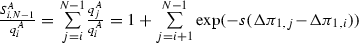
• The fixation probabilities $P_{\text {fix}}^A=1/S^A_{0,N-1}$ and $P_{\text {fix}}^B=1/S^B_{0,N-1}$ for strategies A and B, where

  

  (26a)
  

  (26b)

  are rewritten from Eqs. (10) and (14) in terms of the sums in (25b,c).

• The two equivalent formulations for the fixation time

  

  (27a)
  

  (27b)

  where $q^A_0=q^B_0=1$ and indexes i, j and k, l count the number of A and B-strategists, respectively (see Eqs. (12) and (15) and take the transition probabilities (2, 3), and (4, 5) and property (7) into account).

Moreover, we graph in Fig. 5 the quantities in (24) and (25) in six cases with $N=10$ representative of the competition scenarios in Table 1. The figure will support the statements in the proofs. Throughout this “Appendix” we assume a positive intensity of selection ($s>0$).

Fig. 5

Profiles of the payoff differences $\Delta \pi _i$ (linear w.r.t. i, see Eq. (24a), top panel) and of the partial sums $\Delta \pi _{1,j}$ and $\Delta \pi _{N-l,N-1}$ (quadratic with j and l, see Eqs. (25b, c), bottom panel) in the competition scenarios in Table 1 ($N=10$). Recall that, by the linearity of $\Delta \pi _i$, the sum of all payoff differences $\Delta \pi _{1,N-1}$ [Eq. (25a)] is sign equivalent to the sum $\Delta \pi _1+\Delta \pi _{N-1}$ of the first and last differences

Theorem 1

If A/B invades and B/A does not, then A/B fixates and B/A does not.

Proof

We need to prove that if $\Delta \pi _1>0$ and $\Delta \pi _{N-1}>0$ (A invades and B does not), then $P_{\text {fix}}^A>1/N$ and $P_{\text {fix}}^B<1/N$ (A fixates and B does not). The other case ($\Delta \pi _1<0$ and $\Delta \pi _{N-1}<0$) follows by the interchange of A and B.

$\Delta \pi _1>0$ and $\Delta \pi _{N-1}>0$ imply $\Delta \pi _{1,j}>0$ and $\Delta \pi _{N-l,N-1}>0$ for all $j,l=1,\ldots ,N-1$ (see gray and white dots in Fig. 5, 1A, respectively). Consequently, all elements in the sum in (26a) are smaller than one and all elements in the sum in (26b) are larger than one. We hence have $P_{\text {fix}}^A=1/S^A_{0,N-1}>1/N$ and $P_{\text {fix}}^B=1/S^B_{0,N-1}<1/N$.

$\square$

Theorem 2

If neither A nor B fixate, then neither A nor B invade.

Proof

We prove the theorem by contradiction, i.e., we show that if at least A or B invades, then at least A or B fixates. If only one strategy invades, the latter statement is true by Theorem 1. It hence remains to be proved that when A and B both invade ($\Delta \pi _1>0$ and $\Delta \pi _{N-1}<0$), then at least A or B fixates ($P_{\text {fix}}^A>1/N$ or $P_{\text {fix}}^B>1/N$).

Assume then $\Delta \pi _1>0$ and $\Delta \pi _{N-1}<0$. If $\Delta \pi _1+\Delta \pi _{N-1}>0$, i.e., $\Delta \pi _{1,N-1}>0$, then $\Delta \pi _{1,j}>0$ for all $j=1,\ldots ,N-1$ (see gray dots in Fig. 5, 2A), so that all elements in the sum in (26a) are smaller than one and $P_{\text {fix}}^A=1/S^A_{0,N-1}>1/N$ (A fixates). Vice versa, if $\Delta \pi _1+\Delta \pi _{N-1}<0$, i.e., $\Delta \pi _{1,N-1}<0$, then $\Delta \pi _{N-l,N-1}<0$ for all $l=1,\ldots ,N-1$ (see white dots in Fig. 5, 2B), so that all elements in the sum in (26b) are smaller than one and $P_{\text {fix}}^B=1/S^B_{0,N-1}>1/N$ (B fixates). $\square$

Theorem 3

If A and B both fixate, then A and B both invade.

Proof

We prove the theorem by contradiction, i.e., we show that if at least A or B does not invade, then at least A or B does not fixate. If only one strategy invades, the latter statement is true by Theorem 1. It hence remains to be proved that when neither A nor B invade ($\Delta \pi _1<0$ and $\Delta \pi _{N-1}>0$), then at least A or B does not fixate ($P_{\text {fix}}^A<1/N$ or $P_{\text {fix}}^B<1/N$).

Assume then $\Delta \pi _1<0$ and $\Delta \pi _{N-1}>0$. If $\Delta \pi _1+\Delta \pi _{N-1}>0$, i.e., $\Delta \pi _{1,N-1}>0$, then $\Delta \pi _{N-l,N-1}>0$ for all $l=1,\ldots ,N-1$ (see white dots in Fig. 5, 7A), so that all elements in the sum in (26b) are larger than one and $P_{\text {fix}}^B=1/S^B_{0,N-1}<1/N$ (B does not fixate). Vice versa, if $\Delta \pi _1+\Delta \pi _{N-1}<0$, i.e., $\Delta \pi _{1,N-1}<0$, then $\Delta \pi _{1,j}<0$ for all $j=1,\ldots ,N-1$ (see gray dots in Fig. 5, 7B), so that all elements in the sum in (26a) are larger than one and $P_{\text {fix}}^A=1/S^A_{0,N-1}<1/N$ (A does not fixate). $\square$

Theorem 4 addresses the limit $N\rightarrow \infty$. For this, we consider the frequency $x=i/N$ (or $x=j/N$) of A-strategists and the frequency $1-x=k/N$ (or $1-x=l/N$) of B-strategists, and we rewrite the payoff differences in (24) and the sums in (25) for large N as

$$\begin{aligned} \Delta \pi (x)= & {} \pi _A(x)-\pi _B(x)=\lim _{N\rightarrow \infty }\Delta \pi _i|_{i=xN} = (b-d)(1-x)+(a-c)x, \nonumber \\\end{aligned}$$

(28a)

$$\begin{aligned} \Delta \pi (0)= & {} b-d,\quad \Delta \pi (1)= a-c, \end{aligned}$$

(28b)

and

(29a)

(29b)

(29c)

We also recall the limits for large N of the transition probabilities (2, 3) and (4, 5), i.e.,

$$\begin{aligned} T^+(x)=\lim _{N\rightarrow \infty }T^+_i|_{i=xN}=\left\{ \begin{array}{ll} \frac{x(1-x)}{x+(1-x)\exp (-s\Delta \pi (x))} &{} \text { Moran}\\ \frac{x(1-x)}{1+\exp (-s\Delta \pi (x))} &{} \text { PWC} \end{array}\right. \end{aligned}$$

(30a)

and

$$\begin{aligned} T^-(x)=\lim _{N\rightarrow \infty }T^-_i|_{i=xN}=\left\{ \begin{array}{ll} \frac{x(1-x)}{x\exp (s\Delta \pi (x))+(1-x)} &{} \text { Moran}\\ \frac{x(1-x)}{1+\exp (s\Delta \pi (x))} &{} \text { PWC} \end{array}\right. \end{aligned}$$

(30b)

and the equilibrium frequency (21)

$$\begin{aligned} x^*=(b-d)/(b-d-a+c),\quad 1-x^*=-(a-c)/(b-d-a+c). \end{aligned}$$

(31)

To study the fixation time for large N [following Antal and Scheuring (2006)], we evaluate the sums in (27a) around the frequencies x at which the corresponding elements of the sum diverge with N. Only these dominant elements can give contributions that are more than linear with N and therefore make fixation slow (recall that the fixation time is quadratic with N in the neutral game, $N(N-1)$ and $2N(N-1)$ in the Moran and pairwise comparison cases, respectively).

Before proving Theorem 4, we show the following

Lemma 1

$$\begin{aligned}&\begin{array}{llll} \text {If } b-d>0 &{}\text { and } &{}b-d+a-c>0 &{}\text { then } \lim \limits _{N\rightarrow \infty }S^A_{0,N-1} = \frac{1}{1-\exp (-s(b-d))}.\\ \text {If } b-d<0 &{}\text { or } &{}b-d+a-c<0 &{}\text { then } \lim \limits _{N\rightarrow \infty }S^A_{0,N-1} \approx \exp N.\\ \text {If } a-c<0 &{}\text { and } &{}b-d+a-c<0 &{}\text { then } \lim \limits _{N\rightarrow \infty }S^B_{0,N-1} = \frac{1}{1-\exp (s(a-c))}.\\ \text {If } a-c>0 &{}\text { or } &{}b-d+a-c>0 &{}\text { then } \lim \limits _{N\rightarrow \infty }S^B_{0,N-1} \approx \exp N. \end{array} \end{aligned}$$

Proof

For large N and any finite j, we have $\Delta \pi _{1,j}\approx j(b-d)$ [from (25b)] and [from (25a)]. Under $b-d+a-c>0$, the sum $S^A_{0,N-1}$ is then dominated by the first elements and behaves as a geometric series (convergent if $b-d>0$; divergent if $b-d<0$). Otherwise, if $b-d+a-c<0$, the last elements of $S^A_{0,N-1}$ exponentially diverge with N.

The results on the sum $S^B_{0,N-1}$ similarly follow. For large N and any finite l, we have $\Delta \pi _{N-l,N-1}\approx l(a-c)$ [from (25c)] and (again from (25a)). Under $b-d+a-c<0$, the sum is dominated by the first elements and behaves as a geometric series (convergent if $a-c<0$; divergent if $a-c>0$). Otherwise, if $b-d+a-c<0$, the last elements of $S^B_{0,N-1}$ exponentially diverge with N. $\square$

We also recall that the game classification in Table 3 considers only generic games, i.e., those for which no condition is undetermined.

Theorem 4

For each generic game (a, b, c, d) there is a population size $N^{\infty }$ such that the game classification is as in Table 3 for any $N>N^{\infty }$.

Proof

Separately for each of the five competition scenarios in Table 3, we prove that the corresponding conditions imply the scenario for sufficiently large N. The theorem follows by the fact that the union of the five sets of (mutually exclusive) conditions covers all generic games.

1A :

If $b-d>0$ and $a-c>0$ (A invades and B does not), then, by Lemma 1, $P_{\text {fix}}^A$ and $P_{\text {fix}}^B$ behave for large N as in Table 3. To estimate the fixation time, we use (27a, left) in which we note that $S^A_{0,i-1}$ increases with i from 1 at $i=1$ to $S^A_{0,N-1}$ (finite by Lemma 1) at $i=N$ and that

(32)

decreases with i from $S^A_{0,N-1}$ at $i=0$ to 1 at $i=N-1$ (also note that $\Delta \pi _{1,j}-\Delta \pi _{1,i}>0$ in (32) since $j>i$, see gray dots in Fig. 5, 1A). All terms in (27a, left) but the transition probability $T^+_i$ are therefore positive and bounded for $x\in (0,1)$, whereas $T^+_i$ (at denominator in $t_{\text {fix}}$) vanishes at $x=0$ and $x=1$ [see Eq. (30a)], where it behaves as

$$\begin{aligned} T^+(x)|_{x=0}\approx \left\{ \begin{array}{ll} \frac{x}{\exp (-s(b-d))} &{} \text { Moran}\\ \frac{x}{1+\exp (-s(b-d))} &{} \text { PWC} \end{array}\right. \end{aligned}$$

(33a)

and

$$\begin{aligned} T^+(x)|_{x=1}\approx \left\{ \begin{array}{ll} 1-x &{} \text { Moran} \\ \frac{1-x}{1+\exp (-s(a-c))} &{} \text { PWC} \end{array}\right. \end{aligned}$$

(33b)

The two dominant contributions to $t_{\text {fix}}$ hence come from the elements in (27a, left) around $x=0$ and $x=1$. Using the asymptotic of the Harmonic series, both contributions are proportional to

(34)

1B :

If $b-d<0$ and $a-c<0$ (B invades and A does not), the analysis is symmetric to case 1A (by the interchange of A and B). Specifically, by Lemma 1, $P_{\text {fix}}^A$ and $P_{\text {fix}}^B$ behave for large N as in Table 3. To estimate the fixation time, we use (27a, right) in which we note that $S^B_{0,k-1}$ increases with k from 1 at $k=1$ to $S^B_{0,N-1}$ (finite by Lemma 1) at $k=N$ and that

(35)

decreases with k from $S^B_{0,N-1}$ at $k=0$ to 1 at $k=N-1$ (also note that $\Delta \pi _{N-l,N-1}-\Delta \pi _{N-k,N-1}<0$ in (35) since $l>k$, see white dots in Fig. 5, 1B). All terms in (27a, right) but the transition probability $T^-_{N-k}$ are therefore positive and bounded for $x\in (0,1)$, whereas $T^-_{N-k}$ (at denominator in $t_{\text {fix}}$) behaves for large N as $T^-_{N-k}|_{k=(1-x)N}=T^-_i|_{i=xN}$ and vanishes at $x=0$ and $x=1$ [see Eq. (30b)], where it behaves as

$$\begin{aligned} T^-(x)|_{x=0}\approx \left\{ \begin{array}{ll} x &{} \text { Moran}\\ \frac{x}{1+\exp (s(b-d))} &{} \text { PWC} \end{array}\right. \end{aligned}$$

(36a)

and

$$\begin{aligned} T^-(x)|_{x=1}\approx \left\{ \begin{array}{ll} \frac{1-x}{\exp (s(a-c))} &{} \text { Moran}\\ \frac{1-x}{1+\exp (s(a-c))} &{} \text { PWC} \end{array}\right. \end{aligned}$$

(36b)

The two dominant contributions to $t_{\text {fix}}$ hence come from the elements in (27a, right) around $x=0$ and $x=1$. As in case 1A, both contributions are proportional to $N\log N$.

2A :

If $b-d>0$ and $a-c<0$ with $b-d+a-c>0$ (both A and B invade and selection favors A), then, by Lemma 1, $P_{\text {fix}}^A$ and $P_{\text {fix}}^B$ behave for large N as in case 1A. The fixation time however diverges exponentially due to the contribution of (32) in (27a, left). In fact, while $S^A_{0,i-1}$ and the transition probability $T^+_i$ behave as in case 1A, the difference $\Delta \pi _{1,j}-\Delta \pi _{1,i}$ in (32) is negative for several i, j. The most negative value is attained for $i=i^*$, where $\Delta \pi _{1,i^*}$ is the largest of $\Delta \pi _{1,j}$ (see gray dots in Fig. 5, 2A; $i^*$ corresponds to the last positive $\Delta \pi _i$, see black dots), and for $j=N-1$. For large N, $i^*\approx \lfloor x^*N\rfloor$, where $x^*\in (0,1)$ from (31, left) maximizes the downward parabola $\Delta \pi _{1,j}/N$ in (29b) ($\lfloor i\rfloor$ taking the integer part of i), so that the most negative difference $\Delta \pi _{1,N-1}-\Delta \pi _{1,i^*}$ behaves as $\frac{\scriptstyle N}{\scriptstyle 2}{} \big ((b-d+a-c)-(b-d)^2/(b-d-a+c)\big )$ (obtained from (29b) at $x=1$ and at $x=x^*$). The linear N-dependence of the latter expression makes (32) exponentially diverging with N.

2B :

If $b-d>0$ and $a-c<0$ with $b-d+a-c<0$ (both A and B invade and selection favors B), then, by Lemma 1, $P_{\text {fix}}^A$ and $P_{\text {fix}}^B$ behave for large N as in case 1B. The fixation time however diverges exponentially for large N due to the contribution of (35) in (27a, right). In fact, while $S^B_{0,k-1}$ and the transition probability $T^-_{N-k}$ behave as in case 1B, the difference $\Delta \pi _{N-l,N-1}-\Delta \pi _{N-k,N-1}$ in (35) is positive for several k, l. The most positive value is attained for $k=k^*$, where $\Delta \pi _{N-k^*,N-1}$ is the most negative of $\Delta \pi _{N-l,N-1}$ (see white dots in Fig. 5, 2B; $k^*$ corresponds to the last negative $\Delta \pi _{N-k}$, see black dots), and for $l=N-1$. For large N, $k^*\approx \lfloor (1-x^*)N\rfloor$, where $1-x^*\in (0,1)$ from (31, right) minimizes the upward parabola $\Delta \pi _{N-l,N-1}$ in (29c), so that the most positive difference $\Delta \pi _{1,N-1}-\Delta \pi _{N-k^*,N-1}$ behaves as $\frac{\scriptstyle N}{\scriptstyle 2}{} \big ((b-d+a-c)+(a-c)^2/(b-d-a+c)\big )$ (obtained from (29c) at $1-x=1$ and at $1-x=1-x^*$). The linear N-dependence of the latter expression makes (35) exponentially diverging with N.

3:

If $b-d<0$ and $a-c>0$ (both A and B do not invade), then, by Lemma 1, $P_{\text {fix}}^A$ and $P_{\text {fix}}^B$ behave for large N as in Table 3. To estimate the fixation time, we use (27a, left). If $i\le i^*$, where $\Delta \pi _{1,i^*}$ is the most negative of $\Delta \pi _{1,j}$ (see gray dots in Fig. 5, 3; $i^*$ corresponds to the last negative $\Delta \pi _i$, see black dots), we exploit $q^A_i=(T^-_i/T^+_i)q^A_{i-1}$ and rewrite the element of the sum (27a, left) as

(37)

In (37), we note that $\lim _{N\rightarrow \infty }S^A_{i,N-1}/S^A_{0,N-1}=1$, as the sums $S^A_{i,N-1}$ and $S^A_{0,N-1}$ are dominated for large N by the same element at $j=i^*$, that

(38)

increases with i from 1 at $i=1$ to $1/(1-\exp (s(b-d)))$ at $i=i^*$ (using $\Delta \pi _{1,j}-\Delta \pi _{1,i-1}\approx -(i-1-j)(b-d)>0$ from (25b) for large N and noting that $i^*\approx \lfloor x^*N\rfloor$ diverges with N, so the sum in (38) is a convergent geometric series), and that $T^-_i$ at denominator behaves as in (30b). If $i>i^*$, we directly use (27a, left) in which $\lim _{N\rightarrow \infty }S^A_{0,i-1}/S^A_{0,N-1}=1$, as the sums $S^A_{0,i-1}$ and $S^A_{0,N-1}$ are those dominated by the element at $j=i^*$, (32) decreases with i from $1/(1-\exp (-s(a-c)))$ at $i=i^*$ (using $\Delta \pi _{1,j}-\Delta \pi _{1,i}\approx \Delta \pi _{N-(j-i),N-1}\approx (j-i)(a-c)>0$ from (25c) for large N and noting that $N-1-i^*\approx \lfloor (1-x^*)N\rfloor$ diverges with N, so the sum in (32) is a convergent geometric series) to 1 at $i=N-1$, and the transition probability $T^+_i$ at denominator behaves as in (30a).

The dominant elements in (27a, left) are hence those around $x=0$ for $i\ge i^*$, where the transition probability $T^-_i$ vanishes as in (36a), and those around $x=1$ for $i>i^*$, where the transition probability $T^+_i$ vanishes as in (33b). As in case 1A, both contributions to $t_{\text {fix}}$ are proportional to $N\log N$.

$\square$

Theorem 5 addresses the limit $s\rightarrow \infty$. For this, we take the limit for large s of the transition probabilities (2, 3) and (4, 5), obtaining

(39a)

and

(39b)

$i=1,\ldots ,N-1$, and we show the following

Lemma 2

$$\begin{aligned}&\begin{array}{llll} \text {If } \Delta \pi _1>0 &{}\text { and }&{} \Delta \pi _1+\Delta \pi _{N-1}>0 &{}\text { then } \lim \limits _{s\rightarrow \infty }S^A_{0,N-1} = 1.\\ \text {If } \Delta \pi _1<0 &{}\text { or }&{} \Delta \pi _1+\Delta \pi _{N-1}<0 &{}\text { then } \lim \limits _{s\rightarrow \infty }S^A_{0,N-1} \approx \exp s.\\ \text {If } \Delta \pi _{N-1}<0 &{}\text { and }&{} \Delta \pi _1+\Delta \pi _{N-1}<0 &{}\text { then } \lim \limits _{s\rightarrow \infty }S^B_{0,N-1} = 1.\\ \text {If } \Delta \pi _{N-1}>0 &{}\text { or }&{} \Delta \pi _1+\Delta \pi _{N-1}>0 &{}\text { then } \lim \limits _{s\rightarrow \infty }S^B_{0,N-1} \approx \exp s. \end{array} \end{aligned}$$

Proof

The lemma directly follows from the expressions of $S^A_{0,N-1}$ and $S^B_{0,N-1}$ in (26), by noting that the four cases, respectively, correspond to $\Delta \pi _{1,j}>0$ for all $j=1,\ldots ,N-1$, $\Delta \pi _{1,j}<0$ for some j, $\Delta \pi _{N-l,N-1}<0$ for all $l=1,\ldots ,N-1$, and $\Delta \pi _{N-l,N-1}>0$ for some l. $\square$

We also recall that the game classification in Table 4 considers only generic games, i.e., those for which no condition is undetermined.

Theorem 5

For each generic game (a, b, c, d) there is an intensity of selection $s^{\infty }$ such that the game classification is as in Table 4 for any $s>s^{\infty }$.

Proof

Separately for each of the five competition scenarios in Table 4, we prove that the corresponding conditions imply the scenario for sufficiently large s. The theorem follows by the fact that the union of the five sets of (mutually exclusive) conditions covers all generic games.

1A :

If $\Delta \pi _1>0$ and $\Delta \pi _{N-1}>0$ (A invades and B does not), then $\Delta \pi _1+\Delta \pi _{N-1}>0$, so that by Lemma 2 $P_{\text {fix}}^A$ and $P_{\text {fix}}^B$ behave for large s as in Table 4. To estimate the fixation time, we use (27a, left) in which we note that $\lim _{s\rightarrow \infty }S^A_{0,i-1}=\lim _{s\rightarrow \infty }S^A_{0,N-1}=1$, as all elements but the first ($q^A_0=1$) of both sums vanish as $s\rightarrow \infty$, and that $\lim _{s\rightarrow \infty }S^A_{i,N-1}/q^A_i=1$, as $q^A_i$ is the dominant element in $S^A_{i,N-1}$ for large s ($\Delta \pi _{1,i}$ is the smallest of $\Delta \pi _{1,j}$ for $j=i,\ldots ,N-1$, see gray dots in Fig. 5, 1A). Using (39a), the fixation time is then given by

(40)

where the inequalities hold true for $N\ge 3$ (Moran: all elements but the last in the right-most sum are $<1$, the last being $=1$; PWC: all elements in the right-most sum are $<2$, being all $\le N/(N-1)$ that is $<2$ for $N\ge 3$).

1B :

If $\Delta \pi _1<0$ and $\Delta \pi _{N-1}<0$ (B invades and A does not), the analysis is symmetric to case 1A (by the interchange of A and B). Specifically, $\Delta \pi _1+\Delta \pi _{N-1}<0$, so that by Lemma 2 $P_{\text {fix}}^A$ and $P_{\text {fix}}^B$ behave for large s as in Table 4. To estimate the fixation time, we use (27a, right), in which we note that $\lim _{s\rightarrow \infty }S^B_{0,k-1}=\lim _{s\rightarrow \infty }S^B_{0,N-1}=1$, as all elements but the first ($q^B_0=1$) of both sums vanish as $s\rightarrow \infty$, and that $\lim _{s\rightarrow \infty }S^B_{k,N-1}/q^B_k=1$, as $q^B_k$ is the dominant element in $S^B_{k,N-1}$ for large s ($\Delta \pi _{N-k,N-1}$ is the least negative of $\Delta \pi _{N-l,N-1}$ for $l=k,\ldots ,N-1$, see white dots in Fig. 5, 1B). Using (39b) with $i=N-k$, the fixation time then behaves for large s as in case 1A.

2A :

If $\Delta \pi _1>0$ and $\Delta \pi _{N-1}<0$ with $\Delta \pi _1+\Delta \pi _{N-1}>0$ (i.e., with $\Delta \pi _{1,N-1}>0$; both A and B invade and selection favors A), then by Lemma 2 $P_{\text {fix}}^A$ and $P_{\text {fix}}^B$ behave for large s as in Table 4. To show the behavior for large s of the fixation time, we show that the element at $i=i^*$ in (27a, left) exponentially diverges with s, where $\Delta \pi _{1,i^*}$ is the largest of $\Delta \pi _{1,j}$ (see gray dots in Fig. 5, 2A; $i^*$ corresponds to the last positive $\Delta \pi _i$, see black dots). At $i=i^*$, $\lim _{s\rightarrow \infty }S^A_{0,i^*-1}=\lim _{s\rightarrow \infty }S^A_{0,N-1}=1$, as all elements but the first ($q^A_0=1$) of both sums vanish as $s\rightarrow \infty$, $S^A_{i^*,N-1}$ is dominated by its last element $q^A_{N-1}$ ($\Delta \pi _{1,N-1}$ is the smallest of $\Delta \pi _{1,j}$ for $j=i^*,\ldots ,N-1$, see gray dots in Fig. 5, 1A), and $T^+_{i^*}$ is finite from (39a). Consequently, the element at $i=i^*$ in (27a, left) exponentially diverges with s as the ratio $q^A_{N-1}/q^A_{i^*}=\exp (-s(\Delta \pi _{1,N-1}-\Delta \pi _{1,i^*}))$, where $\Delta \pi _{1,N-1}-\Delta \pi _{1,i^*}<0$. Note that other elements in (27a, left) exponentially diverge with s, but this is irrelevant.

2B :

If $\Delta \pi _1>0$ and $\Delta \pi _{N-1}<0$ with $\Delta \pi _1+\Delta \pi _{N-1}<0$ (i.e., with $\Delta \pi _{1,N-1}<0$; both A and B invade and selection favors B), then by Lemma 2 $P_{\text {fix}}^A$ and $P_{\text {fix}}^B$ behave for large s as in Table 4. To show the behavior for large s of the fixation time, we show that the element at $k=k^*$ in (27a, right) exponentially diverges with s, where $\Delta \pi _{N-k^*,N-1}$ is the most negative of $\Delta \pi _{N-l,N-1}$ (see white dots in Fig. 5, 2B; $k^*$ corresponds to the last negative $\Delta \pi _{N-k}$, see black dots). At $k=k^*$, $\lim _{s\rightarrow \infty }S^B_{0,k^*-1}=\lim _{s\rightarrow \infty }S^B_{0,N-1}=1$, as all elements but the first ($q^B_0=1$) of both sums vanish as $s\rightarrow \infty$, $S^B_{k^*,N-1}$ is dominated by its last element $q^B_{N-1}$ ($\Delta \pi _{1,N-1}$ is the least negative of $\Delta \pi _{N-l,N-1}$ for $l=k^*,\ldots ,N-1$, see white dots in Fig. 5, 2B), and $T^-_{N-k^*}=(N-k^*)/N$ from (39a). Consequently, the element at $k=k^*$ in (27a, right) exponentially diverges with s as the ratio $q^B_{N-1}/q^B_{k^*}=\exp (-s(\Delta \pi _{1,N-1}-\Delta \pi _{1,k^*}))$, where $\Delta \pi _{1,N-1}-\Delta \pi _{1,k^*}>0$. Note that other elements in (27a, right) exponentially diverge with s, but this is irrelevant.

3:

If $\Delta \pi _1<0$ and $\Delta \pi _{N-1}>0$ (both A and B do not invade), then by Lemma 2 $P_{\text {fix}}^A$ and $P_{\text {fix}}^B$ behave for large s as in Table 4. To estimate the fixation time, we use (27a, left) and distinguish two intervals of i. If $i\le i^*$ (where $\Delta \pi _{1,i^*}$ is the most negative of $\Delta \pi _{1,j}$, see gray dots in Fig. 5 3), we consider (37) and note that $\lim _{s\rightarrow \infty }S^A_{i,N-1}/S^A_{0,N-1}=1$, as both sums are dominated for large s by the same element at $j=i^*$, and that the ratio in (38) also converges to 1 for large s, $S^A_{0,i-1}$ being dominated by its last element. If $i>i^*$, we directly use (27a, left) in which $\lim _{s\rightarrow \infty }S^A_{0,i-1}/S^A_{0,N-1}=1$, as both sums are dominated by the element at $j=i^*$, and the ratio in (32) also converges to 1 for large s, $S^A_{i,N-1}$ being dominated by its first element. By (39a), the fixation time then given by

(41)

where the inequalities are guaranteed (for $N>3$) similarly to case 1A.

$\square$

References

Altrock PM, Traulsen A (2009) Deterministic evolutionary game dynamics in finite populations. Phys Rev E 80(1):011909
Antal T, Scheuring I (2006) Fixation of strategies for an evolutionary game in finite populations. Bull Math Biol 68(8):1923–1944
Antal T, Nowak MA, Traulsen A (2009) Strategy abundance in games for arbitrary mutation rates. J Theor Biol 257:340–344
Ashcroft P, Traulsen A, Galla T (2015) When the mean is not enough: calculating fixation time distributions in birth–death processes. Phys Rev E 92:042154
Blume LE (1993) The statistical mechanics of strategic interaction. Games Econ Behav 5(3):387–424
Fudenberg D, Nowak MA, Taylor C, Imhof LA (2006) Evolutionary game dynamics in finite populations with strong selection and weak mutation. Theor Popul Biol 70(3):352–363
Han TA, Traulsen A, Gokhale CS (2012) On equilibrium properties of evolutionary multi-player games with random payoff matrices. Theor Popul Biol 81:264–272
Hofbauer J, Sigmund K (1998) Evolutionary games and population dynamics. Cambridge University Press, Cambridge
Maynard Smith J (1982) Evolution and the theory of games. Cambridge University Press, Cambridge
Maynard Smith J, Price J (1973) The logic of animal conflicts. Nature 246:15–18
Nowak MA (2006) Evolutionary dynamics. Harvard University Press, Cambridge
Nowak MA, Sasaki A, Taylor C, Fudenberg D (2004) Emergence of cooperation and evolutionary stability in finite populations. Nature 428:646–650
Sample C, Allen B (2016) The limits of weak selection and large population size in evolutionary game theory. ArXiv:1610.07081 [q-bio.PE]
Szabó G, Tőke C (1998) Evolutionary prisoner’s dilemma game on a square lattice. Phys Rev E 58:69–73
Taylor PJ, Jonker L (1978) Evolutionarily stable strategies and game dynamics. Math Biosci 40:145–156
Taylor C, Fudenberg D, Sasaki A, Nowak MA (2004) Evolutionary game dynamics in finite populations. Bull Math Biol 66(6):1621–1644
Taylor C, Iwasab Y, Nowak MA (2006) A symmetry of fixation times in evolutionary dynamics. J Theor Biol 243:245–251
Traulsen A, Hauert C (2009) Stochastic evolutionary game dynamics. Reviews of nonlinear dynamics and complexity, Vol II. Wiley-VHC, New York, New York, pp 25–61
Traulsen A, Claussen JC, Hauert C (2005) Coevolutionary dynamics: from finite to infinite populations. Physical Rev Lett 95(23):238701
Traulsen A, Nowak MA, Pacheco JM (2006) Stochastic dynamics of invasion and fixation. Phys Rev E 74:011909
Traulsen A, Pacheco JM, Nowak MA (2007) Pairwise comparison and selection temperature in evolutionary game dynamics. J Theor Biol 246(3):522–529
Traulsen A, Shoresh N, Nowak MA (2008) Analytical results for individual and group selection of any intensity. Bull Math Biol 70(5):1410–1424
Wu B, Altrock PM, Wang L, Traulsen A (2010) Universality of weak selection. Phys Rev E 82:046106
Wu B, García J, Hauert C, Traulsen A (2013) Extrapolating weak selection in evolutionary games. PLoS Comput Biol 9(12):e1003381
Wu B, Bauer B, Galla T, Traulsen A (2015) Fitness-based models and pairwise comparison models of evolutionary games are typically different—even in unstructured populations. New J Phys 17:023043
Acknowledgements
We like to thank Arne Traulsen (Max-Planck-Institute for Evolutionary Biology, Plön, Germany) for useful comments on an early draft of this manuscript, and we also acknowledge the contribution of one anonymous reviewer. The work was supported by the Italian Ministry for Education, University, and Research (under contract FIRB RBFR08TIA4).
Author information
Authors and Affiliations
Corresponding author
Additional information
This work was supported by the Italian Ministry for Education, University, and Research (under contract FIRB RBFR08TIA4).