Quintic non-polynomial spline for time-fractional nonlinear Schrödinger equation

Abstract

In this paper, we shall solve a time-fractional nonlinear Schrödinger equation by using the quintic non-polynomial spline and the L1 formula. The unconditional stability, unique solvability and convergence of our numerical scheme are proved by the Fourier method. It is shown that our method is sixth order accurate in the spatial dimension and $(2-\gamma )$th order accurate in the temporal dimension, where γ is the fractional order. The efficiency of the proposed numerical scheme is further illustrated by numerical experiments, meanwhile the simulation results indicate better performance over previous work in the literature.

1 Introduction

In the past few decades, fractional differential equations have gained much importance due to their usefulness in modeling phenomena in various areas such as physics, engineering, finance, biology and chemistry [12, 33, 46, 51]. To cite some recent developments: in 2019 Jajarmi and Baleanu [26] studied a general form of fractional optimal control problems involving fractional derivative with singular or non-singular kernel; Jothimani et al. [30] discussed an exact controllability of nondensely defined nonlinear fractional integrodifferential equations with the Hille–Yosida operator; Valliammal et al. [61] studied the existence of mild solutions of fractional-order neutral differential system with state-dependent delay in Banach space. In 2020 Jajarmi et al. [28] investigated a fractional version of SIRS model for the HRSV disease; Baleanu et al. [2] proposed a new fractional model for the human liver involving the Caputo–Fabrizio fractional derivative; Baleanu et al. [3] studied the fractional features of a harmonic oscillator with position-dependent mass; Sajjadi et al. [54] discussed the chaos control and synchronization of a hyperchaotic model in both the frameworks of classical and of fractional calculus; Jajarmi and Baleanu [27] proposed a new iterative method to generate the approximate solution of nonlinear fractional boundary value problems in the form of uniformly convergent series; Shiri et al. [56] employed discretized collocation methods for a class of tempered fractional differential equations with terminal value problems; Tuan et al. [60] tackled the problem of finding the solution of a multi-dimensional time-fractional reaction-diffusion equation with nonlinear source from the final value data; Li et al. [44] proposed a new approximation for the generalized Caputo fractional derivative based on WSGL formula and solved a generalized fractional sub-diffusion problem; Gao et al. [19] studied the epidemic predictability for the novel coronavirus (2019-nCoV) pandemic by analyzing a time-fractional model and finding its solution by a q-homotopy analysis transform method; Gao et al. [20] investigated the infection system of the novel coronavirus (2019-nCoV) with a nonlocal operator defined in the Caputo sense; Gao et al. [21] tackled the fractional Phi-four equation by using a q-homotopy analysis transform method numerically; Sabir et al. [53] presented a novel meta-heuristic computing solver for solving the singular three-point second-order boundary value problems using artificial neural networks.

The subject of the present work, the Schrödinger equation, was first proposed by the Austrian physicist Erwin Schrödinger in 1926 [55]. It is a fundamental equation in quantum physics that describes the evolution of the position-space wave function of a particle. In fact, the nonlinear Schrödinger equations describe a wide class of physical phenomena such as models of protein dynamics, self-focusing in laser pulses and nonlinear fiber optics [1, 11, 17, 58]. The Schrödinger equation has also been generalized to fractional differential equations. In 2000, Laskin [34] generalized the non-fractional Schrödinger equation to a space-fractional Schrödinger equation by using the Feynman path integrals over the Lévy trajectories and replacing the quantum Riesz derivative with the Laplace operator. Later, in 2004 Naber [50] proposed a different generalization by changing the first order time-derivative to a Caputo fractional derivative—this time-fractional Schrödinger equation has been used to describe fractional quantum mechanical behavior. In 2010, Muslih et al. [49] obtained a fractional Schrödinger equation by using a fractional variational principle and a fractional Klein–Gordon equation. In 2017, Gómez-Aguilar and Baleanu [23] presented an alternative model of fractional Schrödinger equation involving Caputo–Fabrizio fractional operator.

Many researchers pay attention to the numerical treatment of fractional Schrödinger equations. For the space-fractional Schrödinger equation: a linear implicit conservative difference scheme of order $O(\tau ^{2}+h^{2})$ has been proposed in [62] for the case of a coupled nonlinear Schrödinger equation, where τ is the temporal step size and h is the spatial step size; Zhao et al. [65] have used a compact operator to approximate the Riesz derivative, and the proposed linearized difference scheme for a two-dimensional nonlinear space-fractional Schrödinger equation can achieve $O(\tau ^{2}+\bar{h}^{4})$, where $\bar{h}=\max \{h_{1}, h_{2}\}$, $h_{1}$ and $h_{2}$ are the spatial step sizes in the x and y dimensions, respectively; Wang and Huang [64] have presented a conservative linearized difference scheme, which can achieve the order of $O(\tau ^{2}+h^{2})$; a collocation method has been applied to a multi-dimensional space-time variable-order fractional Schrödinger equation in [5]; a fourth-order implicit time-discretization scheme based on the exponential time differencing approach together with a fourth-order compact scheme in space have been proposed in [31], the method is of order $O(\tau ^{4}+h^{4})$; Li et al. [37] have used a fast linearized conservative finite element method to solve the coupled type equation; Wang and Xiao [63] have proposed an efficient conservative scheme for the fractional Klein–Gordon–Schrödinger equation with central difference and Crank–Nicolson scheme, their method can achieve $O(\tau ^{2}+h^{2})$. It is also noted that Hashemi and Akgül [24] have utilized Nucci’s reduction method and the simplest equation method to extract analytical solutions specially of soliton kinds of nonlinear Schrödinger equations in both time and space fractional terms.

For the time-fractional Schrödinger equation: Khan et al. [32] have applied the homotopy analysis method; Mohebbi et al. [47] have used the Kansa approach to approximate the spatial derivative and L1 discretization to approximate the Caputo time-fractional derivative; a Krylov projection method has been developed in [22]; a Jacobi spectral collocation method has been applied to a multi-dimensional time-fractional Schrödinger equation in [4]; a quadratic B-spline Galerkin method combined with L1 discretization scheme has been proposed in [16]; a linearized L1-Galerkin finite element method has been used in [35] for a multi-dimensional nonlinear time-fractional Schrödinger equation; a cubic non-polynomial spline method combined with L1 discretization has been proposed in [36] and the stability has been shown by the Fourier method, the convergence order is not proved but is observed from numerical experiments to be $O(\tau ^{2-\gamma }+h^{4})$.

Motivated by the above research, in this paper we consider the following time-fractional nonlinear Schrödinger equation:

$$ \textstyle\begin{cases}\displaystyle i\,{}^{C}_{0}{D}^{\gamma }_{t} u(x,t)+ \frac{\partial ^{2} u(x,t)}{\partial x^{2}}+\lambda \big\vert u(x,t) \big\vert ^{2} u(x,t)=f(x,t), \quad (x,t)\in [0,L]\times [0,T], \\ u(x,0)=A_{0}(x), \quad x\in [0,L], \\ u(0,t)=A_{1}(t), \qquad u(L,t)=A_{2}(t), \quad t\in [0,T], \end{cases} $$

(1.1)

where λ is a real constant, $f(x,t)$, $A_{0}(x)$, $A_{1}(t)$, $A_{2}(t)$ are continuous functions with $A_{0}(0)=A_{1}(0)$ and $A_{0}(L)=A_{2}(0)$, and ${}^{C}_{0}{D}^{\gamma }_{t} u(x,t)$ is the Caputo fractional derivative of order $\gamma \in (0,1)$ defined by [12, 51]

$$ {}^{C}_{0}{D}^{\gamma }_{t} u(x,t)= \frac{1}{\Gamma (1-\gamma )} \int _{0}^{t} (t-s)^{-\gamma } \frac{\partial u(x,s)}{\partial s}\,ds. $$

(1.2)

We shall employ a quintic non-polynomial spline together with L1 discretization to solve (1.1). The stability, unique solvability and convergence of our numerical scheme are then proved by the Fourier method—we note that this method of proof is rare for numerical methods of time/space-fractional Schrödinger equation, especially in establishing the convergence order; on the other hand, the energy method has been commonly used to show the convergence of numerical methods for space-fractional Schrödinger equation [31, 62–65]. By the Fourier method, it is shown that our method is of order $O(\tau ^{2-\gamma }+h^{6})$—this improves the spatial convergence achieved by other methods for time-fractional Schrödinger equation. Further, on the choices of our tools, we have observed in several different problems that a non-polynomial spline usually exhibits a better approximation than a polynomial spline because of its parameter [13, 15, 25, 38–43, 52, 57]; while L1 discretization is a stable and widely used approximation for the Caputo fractional derivative [15, 18, 29, 38, 48].

The organization of this paper is as follows. We derive the numerical scheme in Sect. 2. The stability, unique solvability and convergence are established by the Fourier method in Sects. 3, 4 and 5 respectively. In Sect. 6, we present three examples to verify the efficiency of our numerical scheme and to compare with other methods in the literature. Finally, a conclusion is drawn in Sect. 7.

2 Derivation of the numerical scheme

In this section, we shall develop a numerical scheme for problem (1.1) by using quintic non-polynomial spline and L1 discretization. The details of quintic non-polynomial spline will be presented first.

Let

$$ \bar{P}: 0=x_{0}< x_{1}< \cdots < x_{M}=L \quad \mbox{and}\quad \bar{P}': 0=t_{0}< t_{1}< \cdots < t_{N}=T $$

(2.1)

be uniform meshes of the spatial interval $[0,L]$ with step size $h=\frac{L}{M}$ and the temporal interval $[0,T]$ with step size $\tau =\frac{T}{N}$, respectively. For any given function $y(x,t)$, we denote $y(x_{j},t_{n})$ by $y_{j}^{n}$, and $y(x_{j},t)$ by $y_{j}$ for fixed t.

Let $u(x,t)$ denote the exact solution of (1.1) and $U_{j}^{n}$ denote the numerical approximation of $u_{j}^{n}$. We shall set $U_{j}^{n}$ to be the value of the quintic non-polynomial spline at $(x_{j},t_{n})$. We define the quintic non-polynomial spline as follows.

Definition 2.1

([57])

Let $t=t_{n}$, $1\leq n \leq N$ be fixed. For a given mesh P̄, we say $P_{n}(x)$ is the quintic non-polynomial spline with parameter $k~(>0)$ if $P_{n}(x) \in C^{(4)}[0,L]$, $P_{n}(x)$ has the form $\operatorname{span}\{1,x,x^{2},x^{3},\sin (kx), \cos (kx)\}$ and its restriction $P_{j,n}(x)$ on $[x_{j},x_{j+1}]$, $0\leq j \leq M-1$ satisfies

$$ \textstyle\begin{cases} P_{j,n}(x_{j})=U_{j}^{n}, \qquad P_{j,n}(x_{j+1})=U_{j+1}^{n}, \\ P^{(2)}_{j,n}(x_{j})=W_{j}^{n}, \qquad P^{(2)}_{j,n}(x_{j+1})=W_{j+1}^{n}, \\ P^{(4)}_{j,n}(x_{j})=F_{j}^{n}, \qquad P^{(4)}_{j,n}(x_{j+1})=F_{j+1}^{n}. \end{cases} $$

(2.2)

From the above definition, we can express $P_{j,n}(x)$ on $[x_{j},x_{j+1}]$, $0\leq j\leq M-1$ as

$$ P_{j,n}(x)=\overline{a}_{j}^{n}+ \overline{b}_{j}^{n}(x-x_{j})+ \overline{c}_{j}^{n}(x-x_{j})^{2}+ \overline{d}_{j}^{n}(x-x_{j})^{3}+ \overline{e}_{j}^{n}\sin k(x-x_{j})+ \overline{f}_{j}^{n}\cos k(x-x_{j}). $$

(2.3)

Denote $\omega =kh$. Using (2.2), a direct computation gives

$$ \begin{aligned} & \overline{a}_{j}^{n}=U_{j}^{n}- \frac{F_{j}^{n}}{k^{4}}, \\ & \overline{b}_{j}^{n}=\frac{U_{j+1}^{n}-U_{j}^{n}}{h}+ \frac{F_{j}^{n}-F_{j+1}^{n}}{\omega k^{3}}-\frac{h}{6} \bigl(2W_{j}^{n}+W_{j+1}^{n} \bigr)- \frac{h}{6k^{2}} \bigl(2F_{j}^{n}+F_{j+1}^{n} \bigr), \\ & \overline{c}_{j}^{n}=\frac{1}{2} \biggl(W_{j}^{n}+ \frac{F_{j}^{n}}{k^{2}} \biggr), \\ & \overline{d}_{j}^{n}=\frac{W_{j+1}^{n}-W_{j}^{n}}{6h}+ \frac{F_{j+1}^{n}-F_{j}^{n}}{6\omega k}, \\ & \overline{e}_{j}^{n}= \frac{F_{j+1}^{n}-F_{j}^{n}\cos \omega }{k^{4}\sin \omega }, \\ & \overline{f}_{j}^{n}=\frac{F_{j}^{n}}{k^{4}}. \end{aligned} $$

(2.4)

Using the continuity of the first and third derivatives of the spline at $x=x_{j+1}$, i.e., $P^{(1)}_{j,n}(x_{j+1})=P^{(1)}_{j+1,n}(x_{j+1})$ and $P^{(3)}_{j,n}(x_{j+1})=P^{(3)}_{j+1,n}(x_{j+1})$, we obtain the following relations for $1\leq j\leq M-1$:

$$ \begin{aligned} (\mathrm{a})&\quad W_{j-1}^{n}+4W_{j}^{n}+W_{j+1}^{n} \\ &\hphantom{(\mathrm{a})}\quad = \frac{6}{h^{2}} \bigl(U_{j-1}^{n}-2U_{j}^{n}+U_{j+1}^{n} \bigr)-6h^{2} \bigl(\alpha _{1}F_{j-1}^{n}+2 \beta _{1}F_{j}^{n}+\alpha _{1}F_{j+1}^{n} \bigr), \\ (\mathrm{b})&\quad W_{j-1}^{n}-2W_{j}^{n}+W_{j+1}^{n}=h^{2} \bigl( \alpha F_{j-1}^{n}+2\beta F_{j}^{n}+ \alpha F_{j+1}^{n} \bigr), \end{aligned} $$

(2.5)

where

$$ \begin{aligned} & \alpha =\frac{1}{\omega ^{2}} \biggl( \frac{\omega }{\sin \omega }-1 \biggr), \qquad {}\beta = \frac{1}{\omega ^{2}} \biggl(1- \frac{\omega \cos \omega }{\sin \omega } \biggr), \\ & \alpha _{1}=\frac{1}{6\omega ^{2}}+ \frac{1}{\omega ^{4}}- \frac{1}{\omega ^{3} \sin \omega }, \qquad {}\beta _{1}=\frac{1}{3\omega ^{2}}-1+ \frac{\cos \omega }{\omega ^{3} \sin \omega }. \end{aligned} $$

(2.6)

Note that the consistency relation for (2.5)(b) will lead to $2(\alpha +\beta )=1$. Manipulating (2.5)(a) and (2.5)(b), we can easily get

$$ \begin{aligned} &p W_{j+2}^{n}+q W_{j+1}^{n}+s W_{j}^{n}+q W_{j-1}^{n}+p W_{j-2}^{n} \\ &\quad = \frac{1}{h^{2}} \bigl[\alpha U_{j+2}^{n}+2( \beta - \alpha )U_{j+1}^{n}+2(\alpha -2\beta )U_{j}^{n}+2(\beta -\alpha )U_{j-1}^{n}+ \alpha U_{j-2}^{n} \bigr], \\ &\qquad 2\leq j \leq M-2, \end{aligned} $$

(2.7)

where

$$ p=\alpha _{1}+\frac{\alpha }{6},\qquad q=2 \biggl[ \frac{2\alpha +\beta }{6}-(\alpha _{1}-\beta _{1}) \biggr],\qquad s=2 \biggl[\frac{\alpha +4\beta }{6}+(\alpha _{1}-2\beta _{1}) \biggr]. $$

(2.8)

Using the quintic non-polynomial spline to approximate the exact solution $u(x,t)$ of (1.1), the spline relation (2.7) leads to

$$ \begin{aligned} & p \frac{\partial ^{2} u_{j+2}^{n}}{\partial x^{2}}+q \frac{\partial ^{2} u_{j+1}^{n}}{\partial x^{2}}+s \frac{\partial ^{2} u_{j}^{n}}{\partial x^{2}}+q \frac{\partial ^{2} u_{j-1}^{n}}{\partial x^{2}}+p \frac{\partial ^{2} u_{j-2}^{n}}{\partial x^{2}} \\ &\quad = \frac{1}{h^{2}} \bigl[\alpha u_{j+2}^{n}+2( \beta - \alpha )u_{j+1}^{n}+2(\alpha -2\beta )u_{j}^{n}+2(\beta -\alpha )u_{j-1}^{n}+ \alpha u_{j-2}^{n} \bigr]+\Upsilon _{j}^{n}, \\ &\qquad 2\leq j \leq M-2, \end{aligned} $$

(2.9)

where $\Upsilon _{j}^{n}$ is the local truncation error in the spatial dimension. The next lemma gives a result on this error.

Lemma 2.1

For any fixed $t=t_{n}$, $1\leq n\leq N$, let $u(x,t_{n})\in C^{(8)}[0,L]$. If

$$ p=\frac{1}{12}\alpha -\frac{1}{240},\qquad q=\frac{2}{3} \alpha + \frac{1}{10},\qquad s=-\frac{3}{2}\alpha + \frac{97}{120}, $$

(2.10)

then the local truncation error $\Upsilon _{j}^{n}$ associated with the spline relation (2.9) satisfies

$$ \Upsilon _{j}^{n}=O \bigl(h^{6} \bigr),\quad 2 \leq j\leq M-2. $$

(2.11)

Proof

We carry out the Taylor expansion at $x=x_{j}$ in (2.9), this gives

$$ \Upsilon _{j}^{n}=Z_{1} \frac{\partial ^{2} u_{j}^{n}}{\partial x^{2}}+Z_{2} h^{2} \frac{\partial ^{4} u_{j}^{n}}{\partial x^{4}}+Z_{3}h^{4} \frac{\partial ^{6} u_{j}^{n}}{\partial x^{6}}+O \bigl(h^{6} \bigr), $$

where

$$\begin{aligned}& Z_{1}=2(\alpha +\beta )-2p-2q-s,\qquad Z_{2}= \frac{1}{6}(7\alpha + \beta )-4p-q, \\& Z_{3}= \frac{1}{180}(31\alpha +\beta )-\frac{4}{3}p- \frac{1}{12}q. \end{aligned}$$

To achieve the highest order of $O(h^{6})$, we set $Z_{1}=Z_{2}=Z_{3}=0$, which together with the consistency relation $2(\alpha +\beta )=1$, gives (2.10) and (2.11). □

A similar result to Lemma 2.1 has also been obtained in [38].

Remark 2.1

In order to compute the numerical solution $U_{j}^{n}$, $1\leq j\leq M-1$, we need another two equations besides (2.7) or (2.9). We consider the following equations which incorporate the boundary conditions in (1.1):

$$ \begin{aligned} (\mathrm{a})&\quad b_{0} \frac{\partial ^{2} u_{0}^{n}}{\partial x^{2}}+b_{1} \frac{\partial ^{2} u_{1}^{n}}{\partial x^{2}}+b_{2} \frac{\partial ^{2} u_{2}^{n}}{\partial x^{2}}+b_{3} \frac{\partial ^{2} u_{3}^{n}}{\partial x^{2}}+b_{4} \frac{\partial ^{2} u_{4}^{n}}{\partial x^{2}} \\ &\hphantom{(\mathrm{a})} \quad =\frac{1}{h^{2}} \bigl(a_{0}u_{0}^{n}+a_{1}u_{1}^{n}+a_{2}u_{2}^{n}+a_{3}u_{3}^{n}+a_{4}u_{4}^{n} \bigr)+ \Upsilon _{1}^{n}, \\ (\mathrm{b})&\quad b_{M-4} \frac{\partial ^{2} u_{M-4}^{n}}{\partial x^{2}}+b_{M-3} \frac{\partial ^{2} u_{M-3}^{n}}{\partial x^{2}}+b_{M-2} \frac{\partial ^{2} u_{M-2}^{n}}{\partial x^{2}}+b_{M-1} \frac{\partial ^{2} u_{M-1}^{n}}{\partial x^{2}}+b_{M} \frac{\partial ^{2} u_{M}^{n}}{\partial x^{2}} \\ &\hphantom{(\mathrm{b})}\quad =\frac{1}{h^{2}} \bigl(a_{M-4}u_{M-4}^{n}+a_{M-3}u_{M-3}^{n}+a_{M-2}u_{M-2}^{n}+a_{M-1}u_{M-1}^{n}+a_{M}u_{M}^{n} \bigr) \\ &\hphantom{(\mathrm{b})}\qquad{}+ \Upsilon _{M-1}^{n}, \end{aligned} $$

(2.12)

where $\Upsilon _{1}^{n}$ and $\Upsilon _{M-1}^{n}$ are local truncation errors in the spatial dimension, and the constant $a_{i}$ and $b_{i}$ have to be computed such that

$$ \Upsilon _{j}^{n}=O \bigl(h^{6} \bigr),\quad j=1, M-1. $$

(2.13)

By carrying out Taylor expansion at $x=x_{2}$ and $x=x_{M-2}$ in (2.12)(a) and (2.12)(b), respectively, we get the following which satisfies (2.13):

$$\begin{aligned}& (a_{0},a_{1},a_{2},a_{3},a_{4})=(a_{M},a_{M-1},a_{M-2},a_{M-3},a_{M-4})= \biggl(\frac{1}{10},\frac{3}{5},-\frac{7}{5}, \frac{3}{5},\frac{1}{10} \biggr), \end{aligned}$$

(2.14)

$$\begin{aligned}& (b_{0},b_{1},b_{2},b_{3},b_{4})=(b_{M},b_{M-1},b_{M-2},b_{M-3},b_{M-4})= \biggl(\frac{1}{240},\frac{1}{6},\frac{79}{120}, \frac{1}{6}, \frac{1}{240} \biggr). \end{aligned}$$

(2.15)

Remark 2.2

If we let the spline parameter $\alpha =\frac{1}{10}$ in (2.9), then $\text{(2.9)}|_{j=2}$ and $\text{(2.9)}|_{j=M-2}$ are simply the same as (2.12)(a) and (2.12)(b), respectively. Therefore, we should have $\alpha \neq \frac{1}{10}$.

To simplify the notations of the spline relations (2.9) and (2.12), we introduce the following definition.

Definition 2.2

For $y=(y_{1},\ldots ,y_{M-1})$, we define the operators ∧ and ∧₁ by

$$ \wedge y_{j}= \textstyle\begin{cases} b_{0}y_{0}+b_{1}y_{1}+b_{2}y_{2}+b_{3}y_{3}+b_{4}y_{4} , &j=1, \\ py_{j-2}+qy_{j-1}+sy_{j}+qy_{j+1}+py_{j+2}, & 2\leq j\leq M-2, \\ b_{M-4}y_{M-4}+b_{M-3}y_{M-3}+b_{M-2}y_{M-2}+b_{M-1}y_{M-1}+b_{M}y_{M} , & j=M-1, \end{cases} $$

and

$$ \wedge _{1} y_{j}= \textstyle\begin{cases} \displaystyle \frac{1}{h^{2}}(a_{0}y_{0}+a_{1}y_{1}+a_{2}y_{2}+a_{3}y_{3}+a_{4}y_{4}), &j=1, \\ \displaystyle \frac{1}{h^{2}}\bigl[\alpha y_{j-2}+2(\beta -\alpha )y_{j-1}+2( \alpha -2\beta )y_{j}+2(\beta -\alpha )y_{j+1}+\alpha y_{j+2}\bigr], & 2 \leq j\leq M-2, \\ \displaystyle \frac{1}{h^{2}}(a_{M-4}y_{M-4}+a_{M-3}y_{M-3}+a_{M-2}y_{M-2}+a_{M-1}y_{M-1}+a_{M}y_{M}), & j=M-1. \end{cases} $$

Remark 2.3

In view of Definition 2.2, (2.11) and (2.13), the spline relations (2.9) and (2.12) can be presented as

$$ \wedge \frac{\partial ^{2} u_{j}^{n}}{\partial x^{2}}=\wedge _{1}u_{j}^{n}+O \bigl(h^{6} \bigr), \quad 1\leq j\leq M-1. $$

(2.16)

The next lemma gives the L1 discretization for the Caputo fractional derivative.

Lemma 2.2

([18, 59])

Let $0<\gamma <1$ and $x=x_{j}$ be fixed. If $u(x_{j},t)\in C^{(2)}[0,t_{n}]$, then we have

$$ {}^{C}_{0}{D}_{t}^{\gamma } u(x_{j},t_{n})=\mu \sum_{k=0}^{n-1} R_{n,k}^{ \gamma } \bigl(u_{j}^{k+1}-u_{j}^{k} \bigr) +O \bigl(\tau ^{2-\gamma } \bigr), $$

(2.17)

where τ is the temporal step size,

$$ \mu =\frac{1}{\tau ^{\gamma }\Gamma (2-\gamma )},\qquad R_{n,k}^{ \gamma }=(n-k)^{1-\gamma }-(n-k-1)^{1-\gamma },\quad 0\leq k \leq n-1. $$

(2.18)

Lemma 2.3

([9, 18])

For $R_{n,k}^{\gamma }$ defined in (2.18), we have

$$ \begin{aligned} (\mathrm{a})&\quad 1=R_{n,n-1}^{\gamma }>R_{n,n-2}^{\gamma }> \cdots >R_{n,k}^{\gamma }> \cdots >R_{n,1}^{\gamma }>R_{n,0}^{\gamma }>0, \\ (\mathrm{b})&\quad R_{n,k}^{\gamma }>\frac{1-\gamma }{(n-k)^{\gamma }},\quad 0 \leq k \leq n-1. \end{aligned} $$

(2.19)

We are now ready to derive the numerical scheme for (1.1). To begin, we discretize (1.1) at $(x_{j},t_{n})$ to get

$$ i\,{}^{C}_{0}{D}^{\gamma }_{t} u(x_{j},t_{n})+ \frac{\partial ^{2} u(x_{j},t_{n})}{\partial x^{2}}+\lambda \bigl\vert u(x_{j},t_{n}) \bigr\vert ^{2} u(x_{j},t_{n})=f(x_{j},t_{n}). $$

(2.20)

Using the L1 discretization (2.17) in (2.20), we obtain

$$ \frac{\partial ^{2} u(x_{j},t_{n})}{\partial x^{2}}=-i\mu \sum_{k=0}^{n-1}R_{n,k}^{ \gamma } \bigl(u_{j}^{k+1}-u_{j}^{k} \bigr)-\lambda \bigl\vert u_{j}^{n} \bigr\vert ^{2}u_{j}^{n}+f_{j}^{n}+O \bigl( \tau ^{2-\gamma } \bigr). $$

(2.21)

Next, applying the operator ∧ to (2.21) yields

$$ \wedge \frac{\partial ^{2} u(x_{j},t_{n})}{\partial x^{2}}=-i\mu \sum_{k=0}^{n-1}R_{n,k}^{\gamma } \bigl(\wedge u_{j}^{k+1}-\wedge u_{j}^{k} \bigr)- \lambda \wedge \bigl( \bigl\vert u_{j}^{n} \bigr\vert ^{2}u_{j}^{n} \bigr)+\wedge f_{j}^{n}+O \bigl( \tau ^{2-\gamma } \bigr). $$

Noting (2.16), it follows that

$$ \wedge _{1} u_{j}^{n}=-i\mu \sum _{k=0}^{n-1}R_{n,k}^{\gamma } \bigl(\wedge u_{j}^{k+1}- \wedge u_{j}^{k} \bigr)-\lambda \wedge \bigl( \bigl\vert u_{j}^{n} \bigr\vert ^{2}u_{j}^{n} \bigr)+\wedge f_{j}^{n}+O \bigl(h^{6}+\tau ^{2-\gamma } \bigr). $$

Upon rearranging the above relation, we have

$$ \begin{aligned} &\wedge _{1} u_{j}^{n}+i\mu \wedge u_{j}^{n}+\lambda \wedge \bigl( \bigl\vert u_{j}^{n} \bigr\vert ^{2}u_{j}^{n} \bigr) \\ &\quad =i\mu \wedge u_{j}^{n-1}-i\mu \sum _{k=0}^{n-2}R_{n,k}^{ \gamma } \bigl(\wedge u_{j}^{k+1}-\wedge u_{j}^{k} \bigr)+\wedge f_{j}^{n}+O \bigl(h^{6}+ \tau ^{2-\gamma } \bigr). \end{aligned} $$

(2.22)

After omitting the error and replacing the exact solution u with the numerical solution U, we get the numerical scheme

$$ \begin{aligned} &\wedge _{1} U_{j}^{n}+i \mu \wedge U_{j}^{n}+\lambda \wedge \bigl( \bigl\vert U_{j}^{n} \bigr\vert ^{2}U_{j}^{n} \bigr) \\ &\quad =i\mu \wedge U_{j}^{n-1}-i\mu \sum _{k=0}^{n-2}R_{n,k}^{ \gamma } \bigl(\wedge U_{j}^{k+1}-\wedge U_{j}^{k} \bigr)+\wedge f_{j}^{n}, \quad 1\leq j\leq M-1, 1\leq n\leq N, \end{aligned} $$

(2.23)

with

$$ \textstyle\begin{cases} U_{j}^{0}=A_{0}(x_{j}), \quad 0\leq j\leq M, \\ U_{0}^{n}=A_{1}(t_{n}), \qquad U_{M}^{n}=A_{2}(t_{n}), \quad 1\leq n \leq N. \end{cases} $$

(2.24)

Remark 2.4

It is obvious that our scheme (2.23) is a nonlinear scheme. To linearize (2.23), following [45] we shall use the iterative algorithm

$$ \begin{aligned} &{}\wedge _{1} U_{j}^{n(r+1)}+i \mu \wedge U_{j}^{n(r+1)}+\lambda \wedge \bigl( \bigl\vert U_{j}^{n(r)} \bigr\vert ^{2}U_{j}^{n(r+1)} \bigr) \\ &\quad =i\mu \wedge U_{j}^{n-1}-i\mu \sum _{k=0}^{n-2}R_{n,k}^{\gamma } \bigl( \wedge U_{j}^{k+1}-\wedge U_{j}^{k} \bigr)+\wedge f_{j}^{n}, \quad 1\leq j \leq M-1, 1\leq n\leq N, \end{aligned} $$

(2.25)

where $U_{j}^{n(r)}$ is the rth iterate of $U_{j}^{n}$, and

$$ U_{j}^{n(0)}= \textstyle\begin{cases} U_{j}^{n-1}, &n=1, \\ 2U_{j}^{n-1}-U_{j}^{n-2}, & 2\leq n\leq N. \end{cases} $$

(2.26)

Note that the scheme (2.25) is linear in $U^{n(r+1)}$. Hence, instead of (2.23)–(2.24), in practice we shall employ the linearized iterative scheme (2.25) with

$$ \textstyle\begin{cases} U_{j}^{0(r+1)}=A_{0}(x_{j}), \quad 0\leq j\leq M, \\ U_{0}^{n(r+1)}=A_{1}(t_{n}),\qquad U_{M}^{n(r+1)}=A_{2}(t_{n}),\quad 1\leq n\leq N. \end{cases} $$

(2.27)

For practical purposes, we would certainly need a stopping criterion to get $U_{j}^{n(r+1)}$ to a desired accuracy. An example of such a stopping criterion is

$$ \frac{ \vert U_{j}^{n(r+1)}-U_{j}^{n(r)} \vert }{ \vert U_{j}^{n(r)} \vert }\leq \mbox{a small constant}. $$

(2.28)

In fact, we shall use the above stopping criterion with the small constant as $1\times 10^{-6}$ for our numerical simulations in Sect. 6.

3 Stability analysis of the numerical scheme

In this section, we shall analyze the stability of the scheme (2.23)–(2.24) via the Fourier method [8, 10]. Noting from Remark 2.4 that in practice we employ the linearized scheme (2.25)–(2.27) instead, effectively this means that in (2.23) we linearize the nonlinear term $|U|^{2}U$ by replacing $|U|^{2}$ with a local constant κ. Note that a similar linearization technique has also been used in [14, 15]. With the linearization, we can rewrite (2.23)–(2.24) as

$$ \textstyle\begin{cases} \wedge _{1} U_{j}^{n}+i\mu \wedge U_{j}^{n}+\lambda \kappa \wedge U_{j}^{n} \\ \quad =i \mu \wedge U_{j}^{n-1}-i\mu \sum_{k=0}^{n-2}R_{n,k}^{\gamma }(\wedge U_{j}^{k+1}- \wedge U_{j}^{k})+\wedge f_{j}^{n},\quad 1\leq j\leq M-1, \\ U_{j}^{0}=A_{0}(x_{j}),\quad 0\leq j\leq M, \\ U_{0}^{n}=A_{1}(t_{n}),\qquad U_{M}^{n}=A_{2}(t_{n}),\quad 1\leq n \leq N. \end{cases} $$

(3.1)

Consider the perturbed system of (3.1) with perturbation in the initial values

$$ \textstyle\begin{cases} \wedge _{1} \hat{U}_{j}^{n}+i\mu \wedge \hat{U}_{j}^{n}+\lambda \kappa \wedge \hat{U}_{j}^{n} \\ \quad =i\mu \wedge \hat{U}_{j}^{n-1}-i\mu \sum_{k=0}^{n-2}R_{n,k}^{ \gamma }(\wedge \hat{U}_{j}^{k+1}-\wedge \hat{U}_{j}^{k})+\wedge f_{j}^{n},\quad 1\leq j\leq M-1, \\ \hat{U}_{j}^{0}=\hat{A}_{0}(x_{j}), \quad 0\leq j\leq M, \\ \hat{U}_{0}^{n}=A_{1}(t_{n}), \qquad \hat{U}_{M}^{n}=A_{2}(t_{n}),\quad 1\leq n\leq N. \end{cases} $$

(3.2)

Let $U_{j}^{n}$ be the solution of (3.1) and let $\hat{U}_{j}^{n}$ be the solution of the perturbed system (3.2). Let $\rho _{j}^{n}={U}_{j}^{n}-\hat{U}_{j}^{n}$, $0\leq j\leq M$, $0 \leq n\leq N$. It follows from (3.1) and (3.2) that

$$ \textstyle\begin{cases} \wedge _{1} \rho _{j}^{n}+i\mu \wedge \rho _{j}^{n}+\lambda \kappa \wedge \rho _{j}^{n} \\ \quad =i\mu \wedge \rho _{j}^{n-1}-i\mu \sum_{k=0}^{n-2}R_{n,k}^{ \gamma }(\wedge \rho _{j}^{k+1}-\wedge \rho _{j}^{k}),\quad 1\leq j \leq M-1, \\ \rho _{j}^{0}= A_{0}(x_{j})-\hat{A}_{0}(x_{j}),\quad 0\leq j\leq M, \\ \rho _{0}^{n}=0, \qquad \rho _{M}^{n}=0,\quad 1\leq n\leq N. \end{cases} $$

(3.3)

Denote $\rho ^{n}=[\rho _{0}^{n},\rho _{1}^{n},\ldots ,\rho _{M}^{n}]$, $0 \leq n\leq N$. Since $\rho _{0}^{n}=\rho _{M}^{n}=0$, we define the L2 norm of $\rho ^{n}$ by

$$ \bigl\Vert \rho ^{n} \bigr\Vert _{2} = \Biggl(\sum _{j=1}^{M-1}h \bigl\vert \rho _{j}^{n} \bigr\vert ^{2} \Biggr)^{\frac{1}{2}}. $$

(3.4)

To apply the Fourier method, we expand $\rho ^{n}$ to a piecewise constant function $\rho ^{n}(x)$, where

$$ \rho ^{n}(x)= \textstyle\begin{cases} \displaystyle \rho _{j}^{n}, & \displaystyle x\in \bigg(x_{j}-\frac{h}{2}, x_{j}+ \frac{h}{2} \bigg], 1\leq j\leq M-1, \\ \displaystyle 0, & \displaystyle x\in \bigg[0,\frac{h}{2} \bigg] \cup \bigg(L- \frac{h}{2}, L \bigg]. \end{cases} $$

(3.5)

Then $\rho ^{n}(x)$ can be expanded as a Fourier series,

$$ \rho ^{n}(x)=\sum_{m=-\infty }^{\infty }d_{n}(m)e^{i2\pi mx/L},\quad 0\leq n\leq N, $$

(3.6)

where

$$ d_{n}(m)=\frac{1}{L} \int _{0}^{L} \rho ^{n}(x)e^{-i2\pi mx/L} \,dx. $$

(3.7)

To carry out the Fourier stability analysis, it is sufficient to consider an individual harmonic of the form [6]

$$ \rho _{j}^{n}(m)=d_{n}(m)e^{i2\pi m jh/L}. $$

Lemma 3.1

Suppose the solution of (3.3) has the following form:

$$ \rho _{j}^{n}(m)=d_{n}(m)e^{i\theta jh}, $$

(3.8)

where $\theta =2\pi m/L$ and m is the wave number. Then the following inequality holds:

$$ \bigl\vert d_{n}(m) \bigr\vert \leq \bigl\vert d_{0}(m) \bigr\vert , \quad 1\leq n\leq N. $$

(3.9)

Proof

For notational simplicity, let $d_{n}\equiv d_{n}(m)$ for a fixed wave number m. We shall use mathematical induction to complete the proof. First, we consider $n=1$. Upon substituting (3.8) into (3.3), we obtain

$$ \wedge _{1} d_{1}e^{i\theta jh}+i\mu \wedge d_{1}e^{i\theta jh}+ \lambda \kappa \wedge d_{1}e^{i\theta jh}=i \mu \wedge d_{0}e^{i \theta jh}. $$

(3.10)

After a series of computations, (3.10) leads to

$$ d_{1}=\Omega d_{0}, $$

(3.11)

where

$$\begin{aligned}& \Omega =\frac{i\eta _{j} }{\phi _{j}+i\eta _{j} }, \end{aligned}$$

(3.12)

$$\begin{aligned}& \eta _{j}= \textstyle\begin{cases} 2b_{0}\mu \cos (2\theta h)+2b_{1}\mu \cos (\theta h)+b_{2}\mu , & j=1, M-1, \\ 2p\mu \cos (2\theta h)+2q\mu \cos (\theta h)+s\mu , & 2\leq j\leq M-2, \end{cases}\displaystyle \end{aligned}$$

(3.13)

and

$$ \phi _{j}= \textstyle\begin{cases} \displaystyle \biggl[ \frac{2a_{0}}{h^{2}}+2b_{0}\lambda \kappa \biggr]\cos (2\theta h)+ \biggl[\frac{2a_{1}}{h^{2}}+2b_{1}\lambda \kappa \biggr]\cos (\theta h) \\ \displaystyle \quad {}+\frac{a_{2}}{h^{2}}+b_{2}\lambda \kappa , & j=1, M-1, \\ \displaystyle \biggl[ \frac{2\alpha }{h^{2}}+2p\lambda \kappa \biggr] \cos (2\theta h)+ \biggl[\frac{4(\beta -\alpha )}{h^{2}}+2q\lambda \kappa \biggr]\cos (\theta h) \\ \displaystyle \quad {}+\frac{2\alpha -4\beta }{h^{2}}+s \lambda \kappa , & 2\leq j\leq M-2. \end{cases} $$

(3.14)

It is obvious that $|\Omega |\leq 1$, therefore from (3.11) we have

$$ \vert d_{1} \vert \leq \vert d_{0} \vert . $$

(3.15)

Next, assume that $|d_{\ell }|\leq |d_{0}|$, $1\leq \ell \leq n-1$. We shall show that $|d_{n}| \leq |d_{0}|$. For any $n\geq 2$, we substitute (3.8) into (3.3) to get

$$ \begin{aligned} &\wedge _{1} d_{n}e^{i\theta jh}+i\mu \wedge d_{n}e^{i\theta jh}+ \lambda \kappa \wedge d_{n}e^{i\theta jh} \\ &\quad =i \mu \wedge d_{n-1}e^{i \theta jh}-i\mu \sum _{k=0}^{n-2}R_{n,k}^{\gamma } \bigl(\wedge d_{k+1}e^{i \theta jh}-\wedge d_{k}e^{i\theta jh} \bigr). \end{aligned} $$

(3.16)

After a series of computations, (3.16) yields

$$ d_{n}=\Omega d_{n-1}- \Omega \sum _{k=0}^{n-2} R_{n,k}^{\gamma }(d_{k+1}-d_{k}), $$

or equivalently

$$ d_{n}=\Omega \Biggl[ \bigl(1-R_{n,n-2}^{\gamma } \bigr)d_{n-1}+\sum_{k=1}^{n-2} \bigl(R_{n,k}^{\gamma }-R_{n,k-1}^{\gamma } \bigr)d_{k}+R_{n,0}^{ \gamma }d_{0} \Biggr]. $$

(3.17)

Using Lemma 2.3, $|d_{\ell }|\leq |d_{0}|$ for $1\leq \ell \leq n-1$, and $|\Omega |\leq 1$, it follows from (3.17) that

$$ \begin{aligned} \vert d_{n} \vert &= \vert \Omega \vert \Biggl\vert \bigl(1-R_{n,n-2}^{\gamma } \bigr)d_{n-1}+\sum_{k=1}^{n-2} \bigl(R_{n,k}^{\gamma }-R_{n,k-1}^{ \gamma } \bigr)d_{k}+R_{n,0}^{\gamma }d_{0} \Biggr\vert \\ &\leq \vert \Omega \vert \Biggl[ \bigl\vert \bigl(1-R_{n,n-2}^{ \gamma } \bigr) \bigr\vert \vert d_{n-1} \vert +\sum _{k=1}^{n-2} \bigl\vert \bigl(R_{n,k}^{ \gamma }-R_{n,k-1}^{\gamma } \bigr) \bigr\vert \vert d_{k} \vert + \bigl\vert R_{n,0}^{ \gamma } \bigr\vert \vert d_{0} \vert \Biggr] \\ &\leq \vert \Omega \vert \Biggl[ \bigl(1-R_{n,n-2}^{\gamma } \bigr) \vert d_{0} \vert +\sum_{k=1}^{n-2} \bigl(R_{n,k}^{\gamma }-R_{n,k-1}^{ \gamma } \bigr) \vert d_{0} \vert +R_{n,0}^{\gamma } \vert d_{0} \vert \Biggr] \\ &= \vert \Omega \vert \vert d_{0} \vert \Biggl[ \bigl(1-R_{n,n-2}^{\gamma } \bigr)+\sum _{k=1}^{n-2} \bigl(R_{n,k}^{\gamma }-R_{n,k-1}^{\gamma } \bigr)+R_{n,0}^{\gamma } \Biggr] \\ &= \vert \Omega \vert \vert d_{0} \vert \leq \vert d_{0} \vert . \end{aligned} $$

(3.18)

Hence, we have completed the proof of (3.9). □

Theorem 3.1

(Stability)

The numerical scheme (2.25)–(2.27) or equivalently (3.1) is unconditionally stable with respect to the initial data.

Proof

From the definition of the L2 norm (3.4) and (3.5), we find

$$ \begin{aligned} \bigl\Vert \rho ^{n} \bigr\Vert _{2} &= \Biggl( \sum_{j=1}^{M-1} h \bigl\vert \rho _{j}^{n} \bigr\vert ^{2} \Biggr)^{\frac{1}{2}} \\ &= \Biggl[ \int _{0}^{h/2} \bigl\vert \rho ^{n}(x) \bigr\vert ^{2}\,dx+ \sum _{j=1}^{M-1} \int _{x_{j}-h/2}^{x_{j}+h/2} \bigl\vert \rho ^{n}(x) \bigr\vert ^{2}\,dx+ \int _{L-h/2}^{L} \bigl\vert \rho ^{n}(x) \bigr\vert ^{2}\,dx \Biggr]^{\frac{1}{2}} \\ &= \biggl[ \int _{0}^{L} \bigl\vert \rho ^{n}(x) \bigr\vert ^{2} \,dx \biggr]^{ \frac{1}{2}}. \end{aligned} $$

(3.19)

Noting the Parseval equality [8, 10]

$$ \int _{0}^{L} \bigl\vert \rho ^{n}(x) \bigr\vert ^{2} \,dx=\sum _{m=-\infty }^{ \infty } \bigl\vert d_{n}(m) \bigr\vert ^{2}, $$

(3.20)

it follows from (3.19) that

$$ \bigl\Vert \rho ^{n} \bigr\Vert _{2}^{2}= \sum_{m=-\infty }^{\infty } \bigl\vert d_{n}(m) \bigr\vert ^{2}. $$

(3.21)

Applying Lemma 3.1 in (3.21), we obtain

$$ \bigl\Vert \rho ^{n} \bigr\Vert _{2}^{2}= \sum_{m=-\infty }^{\infty } \bigl\vert d_{n}(m) \bigr\vert ^{2} \leq \sum _{m=-\infty }^{\infty } \bigl\vert d_{0}(m) \bigr\vert ^{2}= \bigl\Vert \rho ^{0} \bigr\Vert _{2}^{2},\quad 1\leq n\leq N, $$

(3.22)

which shows that the numerical scheme (3.1) is robust to perturbation of initial data. □

4 Solvability of the numerical scheme

In this section, we shall investigate the solvability of the numerical scheme (2.25)–(2.27) or equivalently (3.1). It is clear that the corresponding homogeneous system of (3.1) is

$$ \textstyle\begin{cases} \wedge _{1} U_{j}^{n}+i\mu \wedge U_{j}^{n}+\lambda \kappa \wedge U_{j}^{n} \\ \quad =i \mu \wedge U_{j}^{n-1}-i\mu \sum_{k=0}^{n-2}R_{n,k}^{\gamma }(\wedge U_{j}^{k+1}- \wedge U_{j}^{k}), \quad 1\leq j\leq M-1, \\ U_{j}^{0}=0, \quad 0\leq j\leq M, \\ U_{0}^{n}=0,\qquad U_{M}^{n}=0,\quad 1\leq n\leq N. \end{cases} $$

(4.1)

Similar to the proof of Theorem 3.1, we can verify that the solution of (4.1) satisfies

$$ \bigl\Vert U^{n} \bigr\Vert _{2}\leq \bigl\Vert U^{0} \bigr\Vert _{2},\quad 1\leq n\leq N. $$

Since $U^{0}=0$, it follows that $U^{n}=0$ for $1\leq n\leq N$. Hence, (4.1) has only the trivial solution and we obtain the following theorem.

Theorem 4.1

(Solvability)

The numerical scheme (2.25)–(2.27) or equivalently (3.1) is uniquely solvable.

5 Convergence of the numerical scheme

In this section, we shall establish the convergence of the numerical scheme (2.25)–(2.27) or equivalently (3.1). Recall that $u(x,t)$ is the exact solution of (1.1) and $U_{j}^{n}$ is the numerical approximation of $u_{j}^{n}$ obtained from (3.1). Let the error $E_{j}^{n}$ at $(x_{j},t_{n})$ be $E_{j}^{n}=u_{j}^{n}-U_{j}^{n}$, $0\leq j\leq M$, $0\leq n\leq N$.

Clearly, from (3.1) we obtain the error equation

$$ \begin{aligned} &\wedge _{1} E_{j}^{n}+i \mu \wedge E_{j}^{n}+\lambda \kappa \wedge E_{j}^{n}=i \mu \wedge E_{j}^{n-1}-i \mu \sum_{k=0}^{n-2}R_{n,k}^{\gamma } \bigl(\wedge E_{j}^{k+1}- \wedge E_{j}^{k} \bigr)+T_{j}^{n}, \\ &\quad 1\leq j\leq M-1, 1\leq n\leq N, \end{aligned} $$

(5.1)

where $T_{j}^{n}$ is the local truncation error,

$$ E_{j}^{n}=0, \quad 0\leq j\leq M \quad \mbox{and}\quad E_{0}^{n}=E_{M}^{n}=0, \quad 1\leq n\leq N. $$

Denote $E^{n}=[E_{0}^{n},E_{1}^{n},\ldots ,E_{M}^{n}]$, $0\leq n\leq N$. Since $E_{0}^{n}=E_{M}^{n}=0$, we define the L2 norm of $E^{n}$ by

$$ \bigl\Vert E^{n} \bigr\Vert _{2} = \Biggl(\sum _{j=1}^{M-1}h \bigl\vert E_{j}^{n} \bigr\vert ^{2} \Biggr)^{ \frac{1}{2}}. $$

Likewise, denote $T^{n}=[T_{1}^{n},T_{2}^{n},\ldots ,T_{M-1}^{n}]$, $1\leq n\leq N$ and the L2 norm of $T^{n}$ is given by

$$ \bigl\Vert T^{n} \bigr\Vert _{2} = \Biggl(\sum _{j=1}^{M-1}h \bigl\vert T_{j}^{n} \bigr\vert ^{2} \Biggr)^{ \frac{1}{2}}. $$

In view of (2.16), (2.17) and (2.22), we see that $T_{j}^{n}=O(h^{6}+\tau ^{2-\gamma })$ and there is a constant $C_{1}$ such that

$$ \bigl\vert T_{j}^{n} \bigr\vert \leq C_{1} \bigl(h^{6}+\tau ^{2-\gamma } \bigr),\quad 1\leq j \leq M-1, 1\leq n\leq N. $$

It follows that

$$ \bigl\Vert T^{n} \bigr\Vert _{2}= \Biggl(\sum _{j=1}^{M-1}h \bigl\vert T_{j}^{n} \bigr\vert ^{2} \Biggr)^{ \frac{1}{2}}\leq C_{1}\sqrt{L} \bigl(h^{6}+ \tau ^{2-\gamma } \bigr). $$

(5.2)

Next, similar to (3.5)–(3.7), we define the piecewise constant functions $E^{n}(x)$ and $T^{n}(x)$ by

$$ E^{n}(x)= \textstyle\begin{cases} E_{j}^{n}, & \displaystyle x\in \bigg(x_{j}-\frac{h}{2}, x_{j}+ \frac{h}{2} \bigg], 1\leq j\leq M-1, \\ 0, & \displaystyle x\in \biggl[0,\frac{h}{2} \biggr] \cup \bigg(L- \frac{h}{2}, L \bigg], \end{cases} $$

(5.3)

and

$$ T^{n}(x)= \textstyle\begin{cases} T_{j}^{n}, & \displaystyle x\in \bigg(x_{j}-\frac{h}{2}, x_{j}+ \frac{h}{2} \bigg], 1\leq j\leq M-1, \\ 0, & \displaystyle x\in \biggl[0,\frac{h}{2} \biggr] \cup \bigg(L- \frac{h}{2}, L \bigg]. \end{cases} $$

(5.4)

Then $E^{n}(x)$ and $T^{n}(x)$ have the Fourier series expansions

$$ E^{n}(x)=\sum_{m=-\infty }^{\infty } \epsilon _{n}(m)e^{i2\pi mx/L} ,\qquad T^{n}(x)=\sum _{m=-\infty }^{\infty }\delta _{n}(m)e^{i2\pi mx/L} , $$

(5.5)

where

$$ \epsilon _{n}(m)=\frac{1}{L} \int _{0}^{L} E^{n}(x)e^{-i2\pi mx/L} \,dx, \qquad \delta _{n}(m)=\frac{1}{L} \int _{0}^{L} T^{n}(x)e^{-i2\pi mx/L} \,dx. $$

(5.6)

Similar to (3.19)–(3.21), by applying the Parseval identities we find

$$ \bigl\Vert E^{n} \bigr\Vert _{2}^{2}= \sum_{m=-\infty }^{\infty } \bigl\vert \epsilon _{n}(m) \bigr\vert ^{2},\qquad \bigl\Vert T^{n} \bigr\Vert _{2}^{2}=\sum _{m=-\infty }^{\infty } \bigl\vert \delta _{n}(m) \bigr\vert ^{2}. $$

(5.7)

Further, noting (5.2), we see that $\sum_{m=-\infty }^{\infty }|\delta _{n}(m)|^{2}$ converges and there is a positive constant $C_{2}\geq 1$ [7] such that

$$ \bigl\vert \delta _{n}(m) \bigr\vert \leq C_{2} \bigl\vert \delta _{1}(m) \bigr\vert ,\quad 1\leq n\leq N. $$

(5.8)

As in Sect. 3, we shall consider individual harmonics $E_{j}^{n}(m)$ and $T_{j}^{n}(m)$ of the forms

$$ E_{j}^{n}(m)=\epsilon _{n}(m)e^{i\theta jh},\qquad T_{j}^{n}(m)= \delta _{n}(m)e^{i\theta jh}, $$

(5.9)

where $\theta =2\pi m/L$. Denote $\epsilon _{n}\equiv \epsilon _{n}(m)$ and $\delta _{n}\equiv \delta _{n}(m)$ for a fixed wave number m. Upon substituting (5.9) into (5.1), we get

$$ \begin{aligned} &{}\wedge _{1} \epsilon _{n}e^{i\theta jh}+i\mu \wedge \epsilon _{n}e^{i \theta jh}+ \lambda \kappa \wedge \epsilon _{n}e^{i\theta jh} \\ &\quad =i\mu \wedge \epsilon _{n-1}e^{i\theta jh}-i\mu \sum _{k=0}^{n-2}R_{n,k}^{ \gamma } \bigl(\wedge \epsilon _{k+1}e^{i\theta jh}-\wedge \epsilon _{k}e^{i \theta jh} \bigr)+\delta _{n}e^{i\theta jh}, \\ &\qquad 1\leq j\leq M-1, 1 \leq n\leq N. \end{aligned} $$

(5.10)

Now, we shall present two lemmas which are essential in the proof of the convergence result.

Lemma 5.1

Let $\alpha \in (0,\frac{1}{10} )\cup (\frac{1}{10}, \frac{37}{180} )$. Then we have

$$ \vert s \vert -2 \vert p \vert -2 \vert q \vert >0, $$

(5.11)

where p, q and s are defined in (2.10).

Proof

Recall from Remark 2.2 that $\alpha \neq \frac{1}{10}$. For $\alpha \in (0,\frac{1}{20} )$, we have $p<0$, $q>0$ and $s>0$, therefore

$$ \vert s \vert -2 \vert p \vert -2 \vert q \vert = - \frac{3}{2}\alpha +\frac{97}{120}-2 \biggl( \frac{1}{240}- \frac{1}{12}\alpha \biggr)-2 \biggl( \frac{2}{3} \alpha + \frac{1}{10} \biggr) = - \frac{8}{3}\alpha + \frac{3}{5}>0. $$

For $\alpha \in [\frac{1}{20},\frac{1}{10} )\cup ( \frac{1}{10},\frac{37}{180} )$, we have $p\geq 0$, $q>0$ and $s>0$, therefore

$$ \vert s \vert -2 \vert p \vert -2 \vert q \vert = - \frac{3}{2}\alpha +\frac{97}{120}-2 \biggl( \frac{1}{12} \alpha -\frac{1}{240} \biggr)-2 \biggl( \frac{2}{3} \alpha + \frac{1}{10} \biggr) = -{3}\alpha + \frac{37}{60}>0. $$

The proof is completed. □

Lemma 5.2

Let $\alpha \in (0,\frac{1}{10} )\cup (\frac{1}{10}, \frac{37}{180} )$. Let $\epsilon _{n}$, $1\leq n\leq N$ be the solution of (5.10). Then we have

$$ \vert \epsilon _{n} \vert \leq C_{2}C_{3} \vert \delta _{1} \vert ,\quad 1\leq n\leq N, $$

(5.12)

where $C_{3}=T^{\gamma }\Gamma (1-\gamma )/\overline{C}$ and $\overline{C}=\min \{ \frac{19}{60}, |s|-2|p|-2|q| \}$.

Proof

Since $E^{0}=0$, it is clear from (5.7) that

$$ \epsilon _{0}(m)=\epsilon _{0}=0. $$

(5.13)

We shall first show that (5.12) is true for $n=1$. Indeed, when $n=1$, from (5.10) we get

$$ \epsilon _{1}=\frac{1}{\phi _{j}+i\eta _{j}}\delta _{1}, $$

(5.14)

where $\eta _{j}$ and $\phi _{j}$ are defined in (3.13) and (3.14), respectively.

Next, it is clear from Lemma 5.1 that $\overline{C}>0$. Moreover, we note that $|b_{2}|-2|b_{0}|-2|b_{1}|=\frac{19}{60}$, where $b_{0}$, $b_{1}$ and $b_{2}$ are given in (2.15). Together with (3.13), we obtain

$$ \begin{aligned} \overline{C}&= \min \biggl\{ \frac{19}{60}, \vert s \vert -2 \vert p \vert -2 \vert q \vert \biggr\} \\ &= \min \bigl\{ \vert b_{2} \vert -2 \vert b_{0} \vert -2 \vert b_{1} \vert , \vert s \vert -2 \vert p \vert -2 \vert q \vert \bigr\} \\ &\leq \min \bigl\{ \bigl\vert b_{2}+2b_{0}\cos {(2 \theta h)}+2b_{1} \cos {(\theta h)} \bigr\vert , \bigl\vert s+2p \cos {(2\theta h)}+2q\cos {( \theta h)} \bigr\vert \bigr\} \\ &\leq \frac{1}{\mu } \vert \eta _{j} \vert ,\quad 1\leq j\leq M-1. \end{aligned} $$

(5.15)

Using (5.15), the fact $|\Omega |= \vert \frac{i\eta _{j}}{\phi _{j}+i\eta _{j}} \vert \leq 1$, the definition of μ (Lemma 2.2), Lemma 2.3 and $C_{2}\geq 1$ (refer to (5.8)), we further find from (5.14)

$$\begin{aligned} \vert \epsilon _{1} \vert &= \frac{1}{ \vert \phi _{j}+i\eta _{j} \vert } \vert \delta _{1} \vert \\ &= \frac{C_{3}\overline{C}}{T^{\gamma }\Gamma (1-\gamma )} \frac{1}{ \vert \phi _{j}+i\eta _{j} \vert } \vert \delta _{1} \vert \\ &\leq \frac{C_{3}}{T^{\gamma }\Gamma (1-\gamma )} \frac{ \vert i\eta _{j} \vert }{\mu } \frac{1}{ \vert \phi _{j}+i\eta _{j} \vert } \vert \delta _{1} \vert \\ &= \frac{\tau ^{\gamma }\Gamma (2-\gamma )C_{3}}{T^{\gamma }\Gamma (1-\gamma )} \vert \Omega \vert \vert \delta _{1} \vert \\ &= \frac{1-\gamma }{N^{\gamma }}C_{3} \vert \Omega \vert \vert \delta _{1} \vert < R_{N,0}^{\gamma }C_{3} \vert \Omega \vert \vert \delta _{1} \vert \leq C_{2}C_{3} \vert \delta _{1} \vert . \end{aligned}$$

(5.16)

Hence, we have proved (5.12) for $n=1$.

Now, assume that, for $n\geq 2$,

$$ \vert \epsilon _{\ell } \vert \leq C_{2}C_{3} \vert \delta _{1} \vert ,\quad 1\leq \ell \leq n-1. $$

(5.17)

From (5.10), after a series of computations we get

$$ \epsilon _{n}=\Omega \epsilon _{n-1}- \Omega \sum _{k=0}^{n-2} R_{n,k}^{ \gamma }( \epsilon _{k+1}-\epsilon _{k})+\frac{1}{\phi _{j}+i\eta _{j}} \delta _{n}, $$

or equivalently

$$ \epsilon _{n}=\Omega \Biggl[ \bigl(1-R_{n,n-2}^{\gamma } \bigr) \epsilon _{n-1}+\sum_{k=1}^{n-2} \bigl(R_{n,k}^{\gamma }-R_{n,k-1}^{ \gamma } \bigr)\epsilon _{k}+R_{n,0}^{\gamma }\epsilon _{0} \Biggr] + \frac{1}{\phi _{j}+i\eta _{j}}\delta _{n}. $$

(5.18)

Using (5.13), by a similar argument to (5.16), (5.8), Lemma 2.3, (5.17) and $|\Omega |\leq 1$, it follows from (5.18) that

$$ \begin{aligned} \vert \epsilon _{n} \vert &\leq \vert \Omega \vert \Biggl\vert \bigl(1-R_{n,n-2}^{ \gamma } \bigr)\epsilon _{n-1}+\sum_{k=1}^{n-2} \bigl(R_{n,k}^{ \gamma }-R_{n,k-1}^{\gamma } \bigr)\epsilon _{k}+R_{n,0}^{\gamma } \epsilon _{0} \Biggr\vert +\frac{1}{ \vert \phi _{j}+i\eta _{j} \vert } \vert \delta _{n} \vert \\ &\leq \vert \Omega \vert \Biggl[ \bigl\vert \bigl(1-R_{n,n-2}^{ \gamma } \bigr)\epsilon _{n-1} \bigr\vert + \Biggl\vert \sum _{k=1}^{n-2} \bigl(R_{n,k}^{ \gamma }-R_{n,k-1}^{\gamma } \bigr)\epsilon _{k} \Biggr\vert \Biggr]+R^{\gamma }_{n,0}C_{3} \vert \Omega \vert \vert \delta _{n} \vert \\ &\leq \vert \Omega \vert \Biggl[ \bigl\vert \bigl(1-R_{n,n-2}^{ \gamma } \bigr) \bigr\vert \vert \epsilon _{n-1} \vert +\sum _{k=1}^{n-2} \bigl\vert \bigl(R_{n,k}^{\gamma }-R_{n,k-1}^{\gamma } \bigr) \bigr\vert \vert \epsilon _{k} \vert +R^{\gamma }_{n,0}C_{2}C_{3} \vert \delta _{1} \vert \Biggr] \\ &\leq C_{2}C_{3} \vert \Omega \vert \vert \delta _{1} \vert \Biggl[ \bigl(1-R_{n,n-2}^{ \gamma } \bigr)+\sum_{k=1}^{n-2} \bigl(R_{n,k}^{\gamma }-R_{n,k-1}^{ \gamma } \bigr)+R^{\gamma }_{n,0} \Biggr] \\ &\leq C_{2}C_{3} \vert \delta _{1} \vert . \end{aligned} $$

Hence, we have proved (5.12). □

Theorem 5.1

(Convergence)

Let $\alpha \in (0,\frac{1}{10} )\cup (\frac{1}{10}, \frac{37}{180} )$. Suppose $u(x,t)$ is the exact solution of (1.1) and $u(x,t)\in C^{(8,2)}([0,L]\times [0,T])$. Then we have, for $1\leq n\leq N$,

$$ \bigl\Vert E^{n} \bigr\Vert _{2}=O \bigl(h^{6}+\tau ^{2-\gamma } \bigr). $$

(5.19)

Hence, the numerical scheme (2.25)–(2.27) or equivalently (3.1) is convergent with order $O(h^{6}+\tau ^{2-\gamma })$.

Proof

Using (5.7), Lemma 5.2 and (5.2), we find, for $1\leq n\leq N$,

$$ \begin{aligned} \bigl\Vert E^{n} \bigr\Vert _{2}&= \Biggl(\sum_{m=-\infty }^{\infty } \bigl\vert \epsilon _{n}(m) \bigr\vert ^{2} \Biggr)^{\frac{1}{2}} \\ &\leq C_{2}C_{3} \Biggl(\sum _{m=-\infty }^{\infty } \bigl\vert \delta _{1}(m) \bigr\vert ^{2} \Biggr)^{\frac{1}{2}} \\ &= C_{2}C_{3} \bigl\Vert T^{1} \bigr\Vert _{2} \\ &\leq C_{1}C_{2}C_{3}\sqrt{L} \bigl(h^{6}+\tau ^{2-\gamma } \bigr). \end{aligned} $$

The proof is completed. □

Remark 5.1

As shown in Theorem 5.1, the numerical scheme (2.25)–(2.27) achieves sixth order convergence in the spatial dimension. This improves the work of [36] where the spatial convergence order is observed to be four through numerical experiment. Furthermore, in [36] the authors have only proved the stability of their scheme, while we have proven the stability, unique solvability and convergence of our method by the Fourier method. We remark that the Fourier method is rarely used in the analysis of numerical methods of time/space-fractional Schrödinger equation, especially in establishing the convergence order, so we have successfully illustrated the analytical technique of the Fourier method in this work. It is noted that the energy method has been commonly used to show the convergence of numerical methods for the space-fractional Schrödinger equation [31, 62–65].

6 Numerical examples

In this section, we shall present three numerical examples to verify the efficiency of the scheme (2.25)–(2.27) and to compare with other methods in the literature.

Note that our theoretical convergence result is in L2 norm, nonetheless it would also be interesting to see the convergence in maximum norm. In fact, for a fixed pair of $(h,\tau )$, we shall compute the following accuracy indicators: maximum L2 norm error $E_{2}(h,\tau )$, maximum modulus error $E_{\infty }(h,\tau )$, maximum real part absolute error $E_{\infty }^{\mathrm{Re}}(h,\tau )$ and maximum imaginary part absolute error $E_{\infty }^{\mathrm{Im}}(h,\tau )$, defined by

$$\begin{aligned}& E_{2}(h,\tau )= \max_{0\leq n\leq N} \bigl\Vert E^{n} \bigr\Vert _{2} = \max_{0\leq n \leq N} \Biggl(\sum_{j=1}^{M-1}h \bigl\vert u_{j}^{n}-U_{j}^{n} \bigr\vert ^{2} \Biggr)^{ \frac{1}{2}}, \end{aligned}$$

(6.1)

$$\begin{aligned}& E_{\infty }(h,\tau )= \max_{0\leq n\leq N}\max _{0\leq j \leq M} \bigl\vert u_{j}^{n}-U_{j}^{n} \bigr\vert , \end{aligned}$$

(6.2)

$$\begin{aligned}& \begin{aligned} & E_{\infty }^{\mathrm{Re}}(h,\tau )= \max_{0\leq n\leq N}\max _{0 \leq j \leq M} \bigl\vert \mathrm{Re} \bigl(u_{j}^{n}-U_{j}^{n} \bigr) \bigr\vert , \\ & E_{\infty }^{\mathrm{Im}}(h, \tau )= \max _{0\leq n\leq N} \max_{0\leq j \leq M} \bigl\vert \mathrm{Im} \bigl(u_{j}^{n}-U_{j}^{n} \bigr) \bigr\vert . \end{aligned} \end{aligned}$$

(6.3)

The convergence orders in temporal and spatial dimensions can be computed by

$$\begin{aligned}& \mbox{Temporal}_{2}=\log _{2} \biggl[ \frac{E_{2}(h,2\tau )}{E_{2}(h,\tau )} \biggr],\qquad \mbox{Temporal}_{ \infty }=\log _{2} \biggl[ \frac{E_{\infty }(h,2\tau )}{E_{\infty }(h,\tau )} \biggr], \end{aligned}$$

(6.4)

$$\begin{aligned}& \mbox{Space}_{2}=\log _{2} \biggl[ \frac{E_{2}(2h,\tau )}{E_{2}(h,\tau )} \biggr],\qquad \mbox{Space}_{ \infty }=\log _{2} \biggl[ \frac{E_{\infty }(2h,\tau )}{E_{\infty }(h,\tau )} \biggr]. \end{aligned}$$

(6.5)

Example 6.1

([16, 36, 47])

Consider the time-fractional Schrödinger equation

$$ \textstyle\begin{cases}\displaystyle i\,{}^{C}_{0}{D}^{\gamma }_{t} u(x,t)+ \frac{\partial ^{2} u(x,t)}{\partial x^{2}}+ \big\vert u(x,t) \big\vert ^{2}u(x,t)=f(x,t), \quad (x,t)\in [0,1]\times [0,1], \\ u(x,0)=0, \quad x\in [0,1], \\ u(0,t)=it^{2}, \qquad u(1,t)=it^{2}, \quad t\in [0,1], \end{cases} $$

(6.6)

where $0<\gamma <1$ and

$$ \begin{aligned} f(x,t)&= -\frac{2t^{2-\gamma }}{\Gamma (3-\gamma )}\cos (2 \pi x)+ \bigl(-4\pi ^{2} t^{2}+t^{6} \bigr)\sin (2\pi x) \\ &\quad {} + i \biggl[\frac{2t^{2-\gamma }}{\Gamma (3-\gamma )} \sin (2\pi x)+ \bigl(-4\pi ^{2}t^{2}+t^{6} \bigr)\cos (2\pi x) \biggr]. \end{aligned} $$

(6.7)

The exact solution is $u(x,t)=t^{2}[\sin (2\pi x)+i\cos (2\pi x)]$.

Let $\alpha =1/20$ be fixed. We shall apply the scheme (2.25)–(2.27) to compute the errors and convergence orders, and comparisons are made with other methods in the literature. There follows a brief description of the numerical simulation in Tables 1–4 and Figs. 1–3:

• (i) In Table 1, we fix $h=1/1000$ and let τ vary. Applying (2.25)–(2.27), we compute $E_{2}(h,\tau )$, $E_{\infty }(h,\tau )$ and the respective temporal convergence orders. The numerical results indicate that our method is of order $(2-\gamma )$ in the temporal dimension, thus verifying the theoretical temporal convergence order in Theorem 5.1.

  Table 1 (Example 6.1) $E_{2}(h,\tau )$, $E_{\infty }(h,\tau )$ and temporal convergence orders

• (ii) In Table 2, we fix $\tau =1/5000$ and let h vary. We present $E_{2}(h,\tau )$, $E_{\infty }(h,\tau )$ and the spatial convergence orders of our scheme (2.25)–(2.27) and those of the cubic non-polynomial spline (CNS) method [36]. From Table 2, we see that our method can achieve at least $O(h^{6})$, while the CNS method is $O(h^{4})$. Moreover, our method obtains smaller errors in all the cases. The observation also confirms the theoretical spatial convergence order in Theorem 5.1.

  Table 2 (Example 6.1) $E_{2}(h,\tau )$, $E_{\infty }(h,\tau )$ and spatial convergence orders

• (iii) Let $\tau =1/512$ be fixed. In Table 3, we compare $E^{\mathrm{Re}}_{\infty }(h,\tau )$ and $E^{\mathrm{Im}}_{\infty }(h,\tau )$ of our scheme (2.25)–(2.27) with those of the meshless collocation (MC) method [47] and the CNS method [36]. The numerical results indicate that our method gives the smallest errors in all the cases.

  Table 3 (Example 6.1) Comparing $E^{\mathrm{Re}}_{\infty }(h,\tau )$ and $E^{\mathrm{Im}}_{\infty }(h,\tau )$ with other methods

• (iv) In Table 4, we fix $(h,\tau )=(1/40,1/200)$ and compare $E^{\mathrm{Re}}_{\infty }(h,\tau )$ and $E^{\mathrm{Im}}_{\infty }(h,\tau )$ of our scheme (2.25)–(2.27) with those of the quadratic B-spline Galerkin (QBG) method [16] and the CNS method [36]. Once again, the numerical results show that our scheme outperforms these methods.

  Table 4 (Example 6.1) Comparing $E^{\text{Re}}_{\infty }(h,\tau )$ and $E^{\text{Im}}_{\infty }(h,\tau )$ with other methods

• (v) To visualize the efficiency of our scheme (2.25)–(2.27), we plot the real part (imaginary part) of the numerical solution and exact solution in Fig. 1 (Fig. 2) for $\gamma =0.1$ and $(h,\tau )=(1/16,1/200)$. From the figures, we observe that our method gives a good approximation of the exact solution.

  Figure 1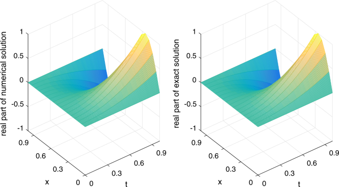

  

  (Example 6.1) Real part of numerical solution and exact solution

  Figure 2

  

  (Example 6.1) Imaginary part of numerical solution and exact solution

• (vi) In Fig. 3, we plot the absolute modulus error $|u_{j}^{n}-U_{j}^{n}|$ obtained from the scheme (2.25)–(2.27) for $\gamma =0.1$ and $(h,\tau )=(1/16,1/200)$. We observe from Fig. 3 that the error is very small.

  Figure 3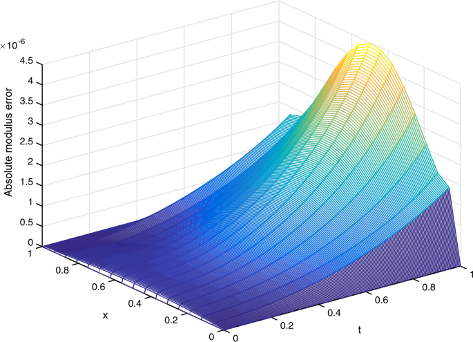

  

  (Example 6.1) Absolute modulus error

Example 6.2

Consider the time-fractional Schrödinger equation

$$ \textstyle\begin{cases} \displaystyle i\,{}^{C}_{0}{D}^{\gamma }_{t} u(x,t)+ \frac{\partial ^{2} u(x,t)}{\partial x^{2}}+ \big\vert u(x,t) \big\vert ^{2}u(x,t)=f(x,t), \quad (x,t)\in [0,1]\times [0,1], \\ u(x,0)=0, \quad x\in [0,1], \\ u(0,t)=it^{\gamma +1}, \qquad u(1,t)=it^{\gamma +1}, \quad t\in [0,1], \end{cases} $$

(6.8)

where $0<\gamma <1$ and

$$ \begin{aligned} f(x,t)&= t\Gamma (\gamma +2) \bigl[i\sin (2\pi x)-\cos (2\pi x) \bigr] \\ &\quad {}+ \bigl(t^{3 \gamma +3}-4\pi ^{2}t^{\gamma +1} \bigr) \bigl[\sin (2\pi x)+i\cos (2\pi x) \bigr]. \end{aligned} $$

(6.9)

The exact solution is $u(x,t)=t^{\gamma +1}[\sin (2\pi x)+i\cos (2\pi x)]$.

Let $\alpha =1/20$ in the implementation of the scheme (2.25)–(2.27). In Table 5, we fix $\tau =1/5000$ and present the spatial convergence orders of our scheme and those of the CNS method [36]. In Table 6, we fix $\tau =1/512$ and compare the maximum real/imaginary part absolute errors of our numerical scheme with those of the CNS method [36]. Furthermore, in Fig. 4 we plot the absolute modulus error $|u_{j}^{n}-U_{j}^{n}|$ obtained from our scheme for $\gamma =0.3$ and $(h,\tau )=(1/20,1/200)$.

Figure 4

(Example 6.2) Absolute modulus error

Table 5 (Example 6.2) $E_{2}(h,\tau )$, $E_{\infty }(h,\tau )$ and spatial convergence orders

Table 6 (Example 6.2) $E^{\text{Re}}_{\infty }(h,\tau )$ and $E^{\text{Im}}_{\infty }(h,\tau )$

From the numerical simulation and plot, once again we demonstrate that the theoretical spatial convergence order of our scheme is at least six (Theorem 5.1) and our scheme performs better than the CNS method.

In the next example, we shall investigate the effect of α on the actual maximum L2 norm error $E_{2}(h,\tau )$.

Example 6.3

Consider the time-fractional Schrödinger equation

$$ \textstyle\begin{cases}\displaystyle i\,{}^{C}_{0}{D}^{\gamma }_{t} u(x,t)+ \frac{\partial ^{2} u(x,t)}{\partial x^{2}}+ \big\vert u(x,t) \big\vert ^{2}u(x,t)=f(x,t), \quad (x,t)\in [0,1]\times [0,1], \\ u(x,0)=0, \quad x\in [0,1], \\ \displaystyle u(0,t)=i\bigl(t^{\gamma +2}-t^{2}\bigr), \qquad u(1,t)=i\bigl(t^{\gamma +2}-t^{2}\bigr), \quad t \in [0,1], \end{cases} $$

(6.10)

where $0<\gamma <1$ and

$$ \begin{aligned} f(x,t)&= \biggl[\frac{\Gamma (\gamma +3)}{\Gamma (3)}t^{2}- \frac{\Gamma (3)}{\Gamma (3-\gamma )}t^{2-\gamma } \biggr] \bigl[i\sin (2 \pi x)-\cos (2\pi x) \bigr] \\ &\quad {} + \bigl[-4\pi ^{2} \bigl(t^{\gamma +2}-t^{2} \bigr)+ \bigl(t^{\gamma +2}-t^{2} \bigr)^{3} \bigr] \bigl[\sin (2\pi x)+i\cos (2\pi x) \bigr]. \end{aligned} $$

(6.11)

The exact solution is $u(x,t)=(t^{\gamma +2}-t^{2})[\sin (2\pi x)+i\cos (2\pi x)]$.

First, we let $\alpha =1/20$ and $\tau =1/5000$ and present the spatial convergence orders of our scheme (2.25)–(2.27) and those of the CNS method [36] (Table 7). To visualize the efficiency of our method, in Figs. 5–7 we plot the real/imaginary parts of the numerical and exact solutions and the absolute modulus error for $\gamma =0.5$ and $(h,\tau )=(1/16,1/200)$. We observe that the theoretical spatial convergence of our method is indeed at least $O(h^{6})$ (Theorem 5.1) and our method gives a good approximation of the exact solution.

Figure 5

(Example 6.3) Real part of numerical solution and exact solution

Figure 6

(Example 6.3) Imaginary part of numerical solution and exact solution

Figure 7

(Example 6.3) Absolute modulus error

Table 7 (Example 6.3) $E_{2}(h,\tau )$, $E_{\infty }(h,\tau )$ and spatial convergence orders

Next, we shall investigate the influence of α on the error $E_{2}(h,\tau )$. Consider the case when $\gamma =0.5$ and $(h,\tau )=(1/10, 1/5000)$. We apply our scheme (2.25)–(2.27) with different values of $\alpha \in (0,\frac{1}{10} )\cup (\frac{1}{10}, \frac{37}{180} )$ and plot the error $E_{2}(h, \tau )$ against α in Fig. 8. It is observed that the exponent of the error remains the same $(10^{-6})$ for all $\alpha \in (0,\frac{1}{10} )\cup (\frac{1}{10}, \frac{37}{180} )$. Noting Table 7, we see that regardless of the chosen value of α, our method (error ∼10⁻⁶) is better than the CNS method (error ∼10⁻⁴) in this case.

Figure 8

(Example 6.3) Influence of α on the error $E_{2}(h,\tau )$

7 Conclusion

In this paper, we derive a numerical scheme to solve the time-fractional nonlinear Schrödinger equation (1.1) of fractional order $\gamma \in (0,1)$. Our tools include the quintic non-polynomial spline and L1 discretization. The unconditional stability, unique solvability and convergence are proved by the Fourier method. It is shown that our method can achieve sixth order convergence in space and $(2-\gamma )$th order convergence in time. Three numerical examples are presented to verify the theoretical results and to compare with other methods in the literature.

References

Agrawal, G.P.: Nonlinear Fiber Optics. Academic Press, San Diego (2001)
Baleanu, D., Jajarmi, A., Mohammadi, H., Rezapour, S.: A new study on the mathematical modelling of human liver with Caputo–Fabrizio fractional derivative. Chaos Solitons Fractals 134, 109705 (2020)
Baleanu, D., Jajarmi, A., Sajjadi, S.S., Asad, J.H.: The fractional features of a harmonic oscillator with position-dependent mass. Commun. Theor. Phys. 72, 055002 (2020)
Bhrawy, A.H., Alzaidy, J.F., Adbelkawy, M.A., Biswas, A.: Jacobi spectral collocation approximation for multi-dimensional time-fractional Schrödinger equations. Nonlinear Dyn. 84, 1553–1567 (2016)
Bhrawy, A.H., Zaky, M.A.: An improved collocation method for multi-dimensional space-time variable-order fractional Schrödinger equations. Appl. Numer. Math. 111, 197–218 (2017)
Charney, J.G., Fjörtoft, R., von Neumann, J.: Numerical integration of the barotropic vorticity equation. Tellus 2, 237–254 (1950)
Chen, C.M., Liu, F., Anh, V., Turner, I.: Numerical schemes with high spatial accuracy for a variable-order anomalous subdiffusion equation. SIAM J. Sci. Comput. 32, 1740–1760 (2010)
Chen, C.M., Liu, F., Turner, I., Anh, V.: A Fourier method for the fractional diffusion equation describing sub-diffusion. J. Comput. Phys. 227, 886–897 (2007)
Chen, S., Liu, F., Zhuang, P., Anh, V.: Finite difference approximations for the fractional Fokker–Planck equation. Appl. Math. Model. 33, 256–273 (2009)
Cui, M.: Compact finite difference method for the fractional diffusion equation. J. Comput. Phys. 228, 7792–7804 (2009)
Dehghan, M., Taleei, A.: A compact split-step finite difference method for solving the nonlinear Schrödinger equations with constant and variable coefficients. Comput. Phys. Commun. 181, 43–51 (2010)
Diethelm, K.: The Analysis of Fractional Differential Equations. Springer, Berlin (2010)
Ding, Q., Wong, P.J.Y.: Mid-knot cubic non-polynomial spline for a system of second-order boundary value problems. Bound. Value Probl. 2018, 156 (2018)
Eilbeck, J.C., McGuire, G.R.: Numerical study of the regularized long-wave equation I: numerical methods. J. Comput. Phys. 19, 43–57 (1975)
El-Danaf, T.S., Hadhoud, A.R.: Parametric spline functions for the solution of the one time fractional Burgers’ equation. Appl. Math. Model. 36, 4557–4564 (2012)
Esen, A., Tasbozan, O.: Numerical solution of time fractional Schrödinger equation by using quadratic B-spline finite elements. Ann. Math. Sil. 31, 83–98 (2017)
Fordy, A.P.: Soliton Theory: A Survey of Results. Manchester University Press, Manchester (1990)
Gao, G.H., Sun, Z.Z.: A compact finite difference scheme for the fractional sub-diffusion equations. J. Comput. Phys. 230, 586–595 (2011)
Gao, W., Veeresha, P., Baskonus, H.M., Prakasha, D.G., Kumar, P.: A new study of unreported cases of 2019-nCOV epidemic outbreaks. Chaos Solitons Fractals 138, 109929 (2020)
Gao, W., Veeresha, P., Prakasha, D.G., Baskonus, H.M.: Novel dynamic structures of 2019-nCoV with nonlocal operator via powerful computational technique. Biology 2020(9), 107 (2020)
Gao, W., Veeresha, P., Prakasha, D.G., Baskonus, H.M., Yel, G.: New numerical results for the time-fractional phi-four equation using a novel analytical approach. Symmetry 2020(12), 478 (2020)
Garrappa, R., Moret, I., Popolizio, M.: Solving the time-fractional Schrödinger equation by Krylov projection methods. J. Comput. Phys. 293, 115–134 (2015)
Gómez-Aguilar, J.F., Baleanu, D.: Schrödinger equation involving fractional operators with non-singular kernel. J. Electromagn. Waves Appl. 31, 752–761 (2017)
Hashemi, M.S., Akgül, A.: Solitary wave solutions of time-space nonlinear fractional Schrödinger’s equation: two analytical approaches. J. Comput. Appl. Math. 339, 147–160 (2018)
Hosseini, S.M., Ghaffari, R.: Polynomial and nonpolynomial spline methods for fractional sub-diffusion equations. Appl. Math. Model. 38, 3554–3566 (2014)
Jajarmi, A., Baleanu, D.: On the fractional optimal control problems with a general derivative operator. Asian J. Control (2019). https://doi.org/10.1002/asjc.2282
Jajarmi, A., Baleanu, D.: A new iterative method for the numerical solution of high-order non-linear fractional boundary value problems. Front. Phys. 8, 220 (2020)
Jajarmi, A., Yusuf, A., Baleanu, D., Inc, M.: A new fractional HRSV model and its optimal control: a non-singular operator approach. Physica A 547, 123860 (2020)
Jin, B., Lazarov, R., Zhou, Z.: Error estimates for a semidiscrete finite element method for fractional order parabolic equations. SIAM J. Numer. Anal. 51, 445–466 (2013)
Jothimani, K., Kaliraj, K., Hammouch, Z., Ravichandran, C.: New results on controllability in the framework of fractional integrodifferential equations with nondense domain. Eur. Phys. J. Plus 134, 441 (2019)
Khaliq, A.Q.M., Liang, X., Furati, K.M.: A fourth-order implicit-explicit scheme for the space fractional nonlinear Schrödinger equations. Numer. Algorithms 75, 147–172 (2017)
Khan, N.A., Jamil, M., Ara, A.: Approximate solutions to time-fractional Schrödinger equation via homotopy analysis method. ISRN Math. Phys. 2012, 197068 (2012)
Kilbas, A.A., Srivastava, H.M., Trujillo, J.J.: Theory and Applications of Fractional Differential Equations. Elsevier, Amsterdam (2006)
Laskin, N.: Fractional quantum mechanics and Lévy path integrals. Phys. Lett. A 268, 298–305 (2000)
Li, D., Wang, J., Zhang, J.: Unconditionally convergent L1-Galerkin FEMs for nonlinear time-fractional Schrödinger equations. SIAM J. Sci. Comput. 39, 3067–3088 (2017)
Li, M., Ding, X., Xu, Q.: Non-polynomial spline method for the time-fractional nonlinear Schrödinger equation. Adv. Differ. Equ. 2018, 318 (2018)
Li, M., Gu, X.M., Huang, C., Fei, M., Zhang, G.: A fast linearized conservative finite element method for the strongly coupled nonlinear fractional Schrödinger equations. J. Comput. Phys. 358, 256–282 (2018)
Li, X., Wong, P.J.Y.: A higher order non-polynomial spline method for fractional sub-diffusion problems. J. Comput. Phys. 328, 46–65 (2017)
Li, X., Wong, P.J.Y.: An efficient numerical treatment of fourth-order fractional diffusion-wave problems. Numer. Methods Partial Differ. Equ. 34, 1324–1347 (2018)
Li, X., Wong, P.J.Y.: A non-polynomial numerical scheme for fourth-order fractional diffusion-wave model. Appl. Math. Comput. 331, 80–95 (2018)
Li, X., Wong, P.J.Y.: An efficient nonpolynomial spline method for distributed order fractional subdiffusion equations. Math. Methods Appl. Sci. 41, 4906–4922 (2018)
Li, X., Wong, P.J.Y.: Non-polynomial spline approach in two-dimensional fractional sub-diffusion problems. Appl. Math. Comput. 357, 222–242 (2019)
Li, X., Wong, P.J.Y.: Numerical solutions of fourth-order fractional sub-diffusion problems via parametric quintic spline. Z. Angew. Math. Mech. 99, e201800094 (2019)
Li, X., Wong, P.J.Y.: A gWSGL numerical scheme for generalized fractional sub-diffusion problems. Commun. Nonlinear Sci. Numer. Simul. 82, 104991 (2020)
Li, X., Zhang, L., Wang, S.: A compact finite difference scheme for the nonlinear Schrödinger equations. Appl. Math. Comput. 219, 3187–3197 (2012)
Meerschaert, M., Scalas, E.: Coupled continuous time random walks in finance. Physica A 370, 114–118 (2006)
Mohebbi, A., Abbaszadeh, M., Dehghan, M.: The use of a meshless technique based on collocation and radial basis functions for solving the time fractional nonlinear Schrödinger equation arising in quantum mechanics. Eng. Anal. Bound. Elem. 37, 475–485 (2013)
Murio, D.A.: Implicit finite difference approximation for time fractional diffusion equations. Comput. Math. Appl. 56, 1138–1145 (2008)
Muslih, S.I., Agrawal, O.P., Baleanu, D.: A fractional Schrödinger equation and its solution. Int. J. Theor. Phys. 49, 1746–1752 (2010)
Naber, M.: Time fractional Schrödinger equation. J. Math. Phys. 45, 3339–3352 (2004)
Podlubny, I.: Fractional Differential Equations. Academic Press, San Diego (1999)
Ramadan, M.A., El-Danaf, T.S., Abd Alaal, F.E.I.: Application of the non-polynomial spline approach to the solution of the Burgers’ equation. Open Appl. Math. J. 1, 15–20 (2007)
Sabir, Z., Baleanu, D., Shoaib, M., Raja, M.A.Z.: Design of stochastic numerical solver for the solution of singular three-point second-order boundary value problems. Neural Comput. Appl. (2020). https://doi.org/10.1007/s00521-020-05143-8
Sajjadi, S.S., Baleanu, D., Jajarmi, A., Pirouz, H.M.: A new adaptive synchronization and hyperchaos control of a biological snap oscillator. Chaos Solitons Fractals 138, 109919 (2020)
Schrödinger, E.: An undulatory theory of the mechanics of atoms and molecules. Phys. Rev. 28, 1049–1070 (1926)
Shiri, B., Wu, G., Baleanu, D.: Collocation methods for terminal value problems of tempered fractional differential equations. Appl. Numer. Math. 156, 385–395 (2020)
Siraj-ul-Islam Tirmizi, I.A., Ashraf, S.: A class of methods based on non-polynomial spline functions for the solution of a special fourth-order boundary-value problems with engineering applications. Appl. Math. Comput. 174, 1169–1180 (2006)
Sulem, C., Sulem, P.L.: The Nonlinear Schrödinger Equation: Self-Focusing and Wave Collapse. Springer, New York (1999)
Sun, Z.Z., Wu, X.: A fully discrete difference scheme for a diffusion-wave system. Appl. Numer. Math. 56, 193–209 (2006)
Tuan, N.H., Baleanu, D., Thach, T.N., O’Regan, D., Can, N.H.: Final value problem for nonlinear time fractional reaction–diffusion equation with discrete data. J. Comput. Appl. Math. 376, 112883 (2020)
Valliammal, N., Ravichandran, C., Hammouch, Z., Baskonus, H.M.: A new investigation on fractional-ordered neutral differential systems with state-dependent delay. Int. J. Nonlinear Sci. Numer. Simul. 20, 803–809 (2019)
Wang, D., Xiao, A., Yang, W.: A linearly implicit conservative difference scheme for the space fractional coupled nonlinear Schrödinger equations. J. Comput. Phys. 272, 644–655 (2014)
Wang, J.J., Xiao, A.G.: An efficient conservative difference scheme for fractional Klein–Gordon–Schrödinger equations. Appl. Math. Comput. 320, 691–709 (2018)
Wang, P., Huang, C.: A conservative linearized difference scheme for the nonlinear fractional Schrödinger equation. Numer. Algorithms 69, 625–641 (2015)
Zhao, X., Sun, Z.Z., Hao, Z.P.: A fourth-order compact ADI scheme for two-dimensional nonlinear space fractional Schrödinger equation. SIAM J. Sci. Comput. 36, 2865–2886 (2014)
Acknowledgements
Not applicable.
Availability of data and materials
Funding
Author information
Authors and Affiliations
Contributions
All the authors contributed equally to the manuscript. All authors read and approved the final manuscript.
Corresponding author
Ethics declarations
Competing interests
The authors declare that they have no competing interests.
Rights and permissions
Open Access This article is licensed under a Creative Commons Attribution 4.0 International License, which permits use, sharing, adaptation, distribution and reproduction in any medium or format, as long as you give appropriate credit to the original author(s) and the source, provide a link to the Creative Commons licence, and indicate if changes were made. The images or other third party material in this article are included in the article’s Creative Commons licence, unless indicated otherwise in a credit line to the material. If material is not included in the article’s Creative Commons licence and your intended use is not permitted by statutory regulation or exceeds the permitted use, you will need to obtain permission directly from the copyright holder. To view a copy of this licence, visit http://creativecommons.org/licenses/by/4.0/.
About this article
Cite this article
Ding, Q., Wong, P.J.Y. Quintic non-polynomial spline for time-fractional nonlinear Schrödinger equation. Adv Differ Equ 2020, 577 (2020). https://doi.org/10.1186/s13662-020-03021-0
Received:
Accepted:
Published:
DOI: https://doi.org/10.1186/s13662-020-03021-0