
Abstract
This paper employs an efficient technique, namely q-homotopy analysis transform method, to study a nonlinear coupled system of equations with Caputo fractional-time derivative. The nonlinear fractional coupled systems studied in this present investigation are the generalized Hirota–Satsuma coupled with KdV, the coupled KdV, and the modified coupled KdV equations which are used as a model in nonlinear physical phenomena arising in biology, chemistry, physics, and engineering. The series solution obtained using this method is proved to be reliable and accurate with minimal computations. Several numerical comparisons are made with well-known analytical methods and the exact solutions when \(\alpha =1\). It is evident from the results obtained that the proposed method outperformed other methods in handling the coupled systems considered in this paper. The effect of the fractional order on the problem considered is investigated, and the error estimate when compared with exact solution is presented.
1 Introduction
The study of fractional calculus, which involves fractional derivatives and integrals, has allured the interest of many in the field of engineering and natural sciences due to its monumental applications such as found in biotechnology [1], chaos theory [2], electrodynamics [3], random walk [4], signal and image processing [5, 6], nanotechnology [7], viscoelasticity [8], and other various fields [9–18]. We also refer the reader to [19–26] for some recent applications of fractional calculus. Many researchers have also described the essential properties of this fractional calculus, see [27–30] for more details. However, solving a fractional coupled system of equations is generally more difficult than the classical type. This is due to the fact that its operators are defined by integral. In the present investigation, we consider the coupled systems: the generalized Hirota–Satsuma coupled with KdV, the coupled KdV, and the modified coupled KdV with Caputo fractional time derivative. Hirota and Satsuma in [31] introduced the coupled KdV equation, while the generalized Hirota–Satsuma coupled KdV and the modified coupled KdV equations were introduced by Wu et al. in [32].
In general, the KdV equations are found in the study of nonlinear dispersive waves [33]. They were introduced in 1895 by Korteweg and de Vries for modeling shallow water waves in a canal [34]. The proposed coupled KdV equations play a prominent role in diverse areas of applied sciences and engineering such as hydrodynamics, plasma physics, water waves, and quantum field theory. They describe the interactions between two long waves with different dispersion relations. These systems have attracted the attention of many researchers, and a great deal of work has been done. For instance, the generalized Hirota–Satsuma coupled with KdV has been handled via different approaches such as the new iterative method (NIM) [35], homotopy perturbation method (HPM) [36], Adomian’ decomposition method (ADM) [37], homotopy analysis (HAM) [38], variational iteration method (VIM) [39], and reduced differential transformation method (RDTM) [40]. Fan in [41] used an extended tanh-function method and symbolic computation to obtain four types of soliton solutions of the generalized Hirota–Satsuma coupled KDV and modified coupled KDV equations. Arife et al. presented the numerical solutions of the generalized Hirota–Satsuma coupled KdV and modified coupled KDV equations through homotopy analysis method (HAM) [42]. In [43], approximate solutions of generalized Hirota–Satsuma coupled KDV and modified coupled KDV equations have been obtained by NIM. Ganji et al. in [44] used modified homotopy perturbation method to solve time-fractional generalized Hirota–Satsuma coupled KdV equations. Ghoreishi et al. used HAM to obtain approximate solutions of modified coupled KdV equations [45]. Kaya and Inan in [46] obtained traveling wave solutions of the coupled KdV and modified coupled KdV equations.
Due to the complicated nature of these coupled systems, the present study employs a combination of q-HAM (a modification of HAM) and the Laplace transform method, named q-homotopy analysis transform method (q-HATM), on these coupled KdV equations. The HAM was proposed in 1992 by Liao [28, 47]. The search for a better way to expand the convergence region led to the modification of HAM, called q-HAM, more of a general method than HAM [48]. Many authors have taken advantage of q-HAM and used it to solve nonlinear fractional partial differential equations [49–55]. The q-HATM was proposed by Singh et al. [56] and did not require any form of discretization, linearization, or perturbation as compared to other methods. It requires neither polynomials like ADM nor Lagrange multiplier like VIM and overcomes the limitations of these methods. The q-HATM uses two convergence parameters ħ and n that provide greater flexibility in adjusting and controlling the convergence region as well as convergence rate of the series solution. With all these advantages, we refer to the q-HATM as a simple, very effective, accurate method that has a wide-ranging feasibility and gives more refined convergent series solution. It is worth mentioning that q-HATM has been used extensively by many researchers due to consistency and efficacy of this method in analyzing nonlinear problems [57–62].
This paper is organized as follows. Some useful definitions, properties, and notations used in the sequel are presented in Sect. 2. The fundamental idea of the proposed method, the convergence theorem, and error analysis are detailed in Sect. 3. Section 4 is focused on the implementation of q-HATM on several examples of coupled KdV system of equations, the effects of fractional order α, and the ħ-curves for optimal choice of the auxiliary parameter h. In Sect. 5, we present comparison of the solutions obtained by the proposed method q-HATM with several other analytical methods such as HPM, NIM, DTM, RDTM using exact solutions as benchmark. Finally, in Sect. 6, we summarize the result in the conclusion.
2 Preliminaries
Here, we present some useful definitions, properties, and notations that will be used in this work.
Definition 2.1
The Riemann–Liouville (R–L) fractional integral of order α (\(\alpha \geq 0\)) of a function \(Q(x,t)\in C_{m}\), \(m\geq {-1}\), is given as [29, 63–65]
where \(J^{0}Q(x,t)=Q(x,t)\) and Γ denotes the classical gamma function. For example,
Definition 2.2
In the Caputo sense the fractional derivative of \(Q(x,t)\) (denoted by \(\mathcal {D}^{\alpha }Q(x,t)\)) for \(\varphi -1<\alpha <\varphi \), \(\varphi \in \mathbb{N}\) is defined as [29, 65]
where
with the following properties:
- a.
\(\mathcal {D}^{\alpha } (\xi _{1}Q(x,t)+\xi _{2}S(x,t) ) =\xi _{1} \mathcal {D}^{\alpha }Q(x,t)+\xi _{2} \mathcal {D}^{\alpha }S(x,t)\), \(\xi _{1},\xi _{2} \in \mathbb{R}\),
- b.
\(\mathcal {D}^{\alpha }J^{\alpha }Q(x,t)=Q(x,t)\),
- c.
\(J^{\alpha }\mathcal {D}^{\alpha }Q(x,t)=Q(x,t)-\sum_{j=0}^{\varphi -1}Q^{j}_{0}(x,t) \frac{t^{j}}{j!}\).
Definition 2.3
The Laplace transform (LT) of a Caputo fractional derivative is given as [27, 65]
3 The q-homotopy analysis transform method (q-HATM)
We first give a general idea of the analysis of q-homotopy analysis transform method (q-HATM) applied to general nonlinear differential equations. Then, some convergence and error analysis theorems are presented.
3.1 Analysis of q-HATM
We give a brief analysis of q-HATM applied to a general nonlinear time-fractional equation of the form
where \(\mathcal {D}_{t}^{\alpha }\) denotes the Caputo fractional derivative, R represents a linear differential operator, \(\mathcal{N}\) indicates the nonlinear differential operator, \(Q(x,t)\) specifies the unknown function, and \(f(x,t)\) is the given source term. Employing Laplace transform denoted by \(\mathscr{L}\) on Equation (5), we obtain
Upon simplification, we reduce Equation (6) to
To epitomize the idea of homotopy method [47], we construct the zeroth-order deformation equations for \(0\leq q \leq \frac{1}{n}\), \(n\geq {1}\), as
where \(\mathcal{N} [\phi (x,t;q) ]\) is defined as
Here, q is the embedded parameter, the nonzero ħ is the auxiliary parameter, and \(\mathcal{H}(x,t)\neq 0\) indicates the auxiliary function. From Equation (8) with \(q=0, \frac{1}{n}\), we obtain
When q rises from 0 to \(\frac{1}{n}\), the solutions \(\phi (x,t;q)\) range from the initial guess \(Q_{0}\) to the solution Q. In case that \(Q_{0}\), \(\mathcal{H}\), and ħ are all chosen accordingly, then the solutions \(\phi (x,t;q)\) in Equation (8) hold in as much as \(0\leq q \leq \frac{1}{n}\). Hence, application of Taylor series expansion [66] for \(\phi (x,t;q)\) gives
where
If we choose \(Q_{0}\), ħ, and \(\mathcal{H}\) adequately in order that Equation (11) converges at \(q=\frac{1}{n}\), from Equation (10) we obtain
Differentiating Equation (8) m-times (w.r.t. to “q”), substituting \(q=0\), then multiplying by \(\frac{1}{m!}\), we obtain
The vector \(\vec{Q}_{r}\) is expressed as
Taking use of the inverse LT on Equation (14), we obtain
where
and
In Equation (17), H denotes homotopy polynomial defined as follows:
3.2 Convergence and error analysis of q-HATM
Here, we give some useful theorems for the purpose of completeness. The detailed proofs can be found in [61, 62] and the references therein.
Theorem 3.1
(Convergence theorem, [61, 62])
Let\(\mathcal{B}\)be a Banach space and\(\mathrm{G}:\mathcal{B}\to \mathcal{B}\)be a nonlinear mapping. Suppose that
where\(0<\mathcal{M}<1\), then G has a fixed point in light of Banach’s fixed point theory [67]. Furthermore, for the arbitrary selection of\(Q_{0}, \hat{Q}_{0}\in \mathcal{B}\), the sequence generated by the q-HATM converges to a fixed point of G and
Theorem 3.2
Suppose that the series solution
defined in Equation (13) is convergent to the solution\(Q(x,t)\)for a prescribed value ofnand ħ. If we can obtain a real number\(0<\rho <1\)satisfying
Moreover, if the truncated series
is used as an approximation to the solutions\(Q(x,t)\)of problem (5), then the maximum absolute truncated errors are estimated as follows:
4 q-HATM application to a coupled system of time-fractional order
We have carefully chosen a coupled system of strongly nonlinear time-fractional differential equations and have applied the q-HATM to obtain the analytical approximate solutions in the form of convergent series.
Example 4.1
Consider the one-dimensional generalized Hirota–Satsuma coupled KdV system of equations [32]
having the initial condition
where k, r, η, and p are arbitrary constants. By implementing LT on Equation (23) with Equation (24), we obtain
The nonlinear operators where \(\phi _{i}=\phi _{i}(x,t;q)\), \(i=1,2,3\), are defined as follows:
Referring to Equation (14) with \(\mathcal{H}(x,t)=1\), the mth-order deformation equation is
where
By employing the inverse LT on Equation (27), we get
On solving the above equation, we obtain the following:
Accordingly, the remaining terms can be derived. Thus, the q-HATM solution is presented as follows:
For the case when \(\alpha =1\), we select \(n=1\), \(\hbar =-1\), and the four-term approximate solution is
which as \(N\to {\infty }\) converges respectively to the exact solutions
Example 4.2
Consider the one-dimensional coupled modified Korteweg–de Vries equation [46]
having initial condition
The solution to the coupled system Equation (33) for a special case when \(\alpha = 1\) is
where λ, k, and r are parameters. By implementing LT on Equation (33), in addition to Equation (34), we obtain
The nonlinear operators where \(\phi _{i}=\phi _{i}(x,t;q)\), \(i=1,2\), are defined as follows:
Referring to Equation (14) with \(\mathcal{H}(x,t)=1\), the mth-order deformation equation is
where
By applying the inverse LT on Equation (38), we have
On solving the above equation and letting \(k=r\), we obtain the following:
Accordingly, the remaining terms can be derived. Thus, the q-HATM solution is presented as follows:
For the case when \(\alpha =1\), we select \(n=1\), \(\hbar =-1\), and the four-term approximate solution is
which as \(N\to {\infty }\) converges respectively to the exact solutions
Example 4.3
Consider the one-dimensional coupled Korteweg–de Vries equation [31, 46]
having initial condition
The solution to the coupled system Equation (44) for a special case when \(\alpha = 1\) is
where \(\mathcal{A}\), \(\mathcal{B}\), and r are real parameters. By implementing LT on Equation (44), in addition to Equation (45), we obtain
The nonlinear operators where \(\phi _{i}=\phi _{i}(x,t;q)\), \(i=1,2\), are define as follows:
Referring to Equation (14) with \(\mathcal{H}(x,t)=1\), the mth-order deformation equation is
where
By applying the inverse LT on Equation (48), we have
On solving the above equation with \(\mathcal{A}=r\) and \(\mathcal{B}=3\), we have
Accordingly, the remaining terms can be derived. Thus, the q-HATM solution is presented as follows:
For the case when \(\alpha =1\), we select \(n=1\), \(\hbar =-1\), and the four-term approximate solution is
which as \(N\to {\infty }\) converges respectively to the exact solutions
4.1 Effects of fractional order α
We study the effect of fractional order α on the solution profiles for the coupled systems considered in this section. The dynamics of the profiles can be clearly observed, and this justifies why these models should be studied to understand these effects in real life applications.
4.2 Optimal choice of auxiliary parameter: ħ-curves
The choice of the auxiliary parameter ħ is very important in the q-HATM to ensure fast convergence of the series solutions. Here, we provide the so-called ħ-curves that guide our optimal choice of the values of ħ in our analysis. Horizontal line test is used to obtain intervals containing optimal values.
Remark 4.1
-
1.
In Figs. 1–14, we present the graphical representation of the obtained results by q-HATM and their respective exact solutions for different fractional order. Our results are in perfect agreement with the exact solutions in the case where \(\alpha =1\). This is an evidence of the fast convergence nature of the series solutions given by q-HATM when the optimal choice of the auxiliary parameter is used. In our computations, \(\hbar =-1\) and \(n=1\) are carefully chosen and used.
Figure 1 
q-HATM vs exact solution when \(\hbar =-1\), \(k=\eta =0.1\), \(r=-1.5\), \(p=1.5\), and \(n=1\) for Example 4.1
Figure 2 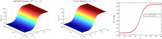
q-HATM vs exact solution when \(\hbar =-1\), \(k=\eta =0.1\), \(r=-1.5\), \(p=1.5\), and \(n=1\) for Example 4.1
Figure 3 
q-HATM vs exact solution when \(\hbar =-1\), \(k=\eta =0.1\), \(r=-1.5\), \(p=1.5\), and \(n=1\) for Example 4.1
Figure 4 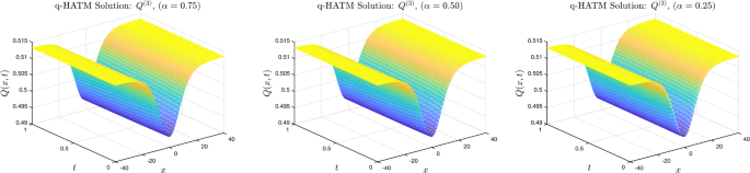
q-HATM \(Q^{(3)}\)-solution with different α when \(\hbar =-1\), \(k=\eta =0.1\), \(r=-1.5\), \(p=1.5\), and \(n=1\) for Example 4.1
Figure 5 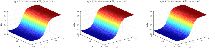
q-HATM \(S^{(3)}\)-solution with different α when \(\hbar =-1\), \(k=\eta =0.1\), \(r=-1.5\), \(p=1.5\), and \(n=1\) for Example 4.1
Figure 6 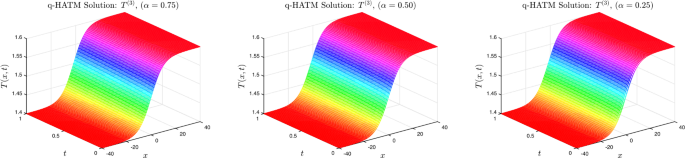
q-HATM \(T^{(3)}\)-solution with different α when \(\hbar =-1\), \(k=\eta =0.1\), \(r=-1.5\), \(p=1.5\), and \(n=1\) for Example 4.1
Figure 7 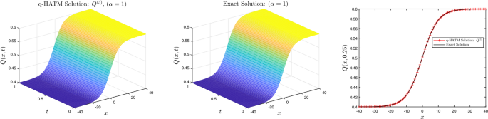
q-HATM vs exact solution when \(\hbar =-1\), \(k=r=0.1\), \(\lambda =1.5\), and \(n=1\) for Example 4.2
Figure 8 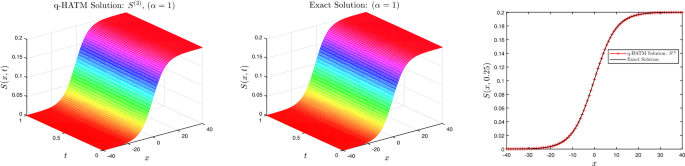
q-HATM vs exact solution when \(\hbar =-1\), \(k=r=0.1\), \(\lambda =1.5\), and \(n=1\) for Example 4.2
Figure 9 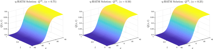
q-HATM \(Q^{(3)}\)-solution with different α when \(\hbar =-1\), \(k=r=0.1\), \(\lambda =1.5\), and \(n=1\) for Example 4.2
Figure 10 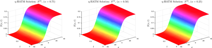
q-HATM \(S^{(3)}\)-solution with different α when \(\hbar =-1\), \(k=r=0.1\), \(\lambda =1.5\), and \(n=1\) for Example 4.2
Figure 11 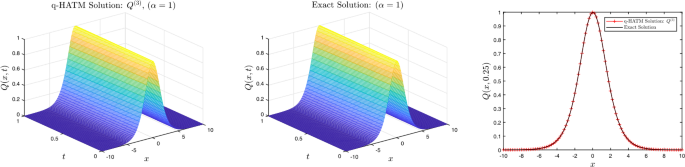
q-HATM vs exact solution when \(\hbar =-1\), \(\mathcal{A}=r=0.1\), \(\mathcal{B}=3\), and \(n=1\) for Example 4.3
Figure 12 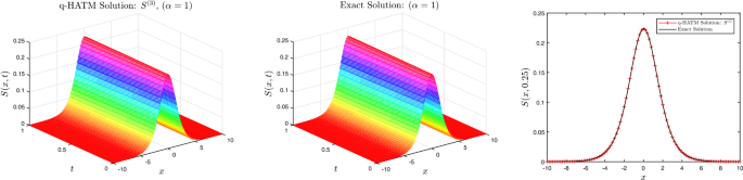
q-HATM vs exact solution when \(\hbar =-1\), \(\mathcal{A}=r=0.1\), \(\mathcal{B}=3\), and \(n=1\) for Example 4.3
Figure 13 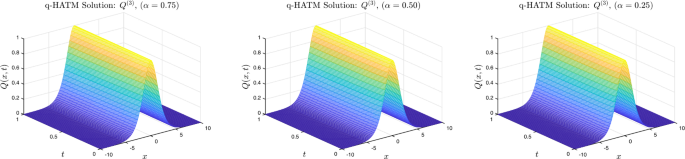
q-HATM \(Q^{(3)}\)-solutions with different α when \(\hbar =-1\), \(\mathcal{A}=r=0.1\), \(\mathcal{B}=3\), and \(n=1\) for Example 4.3
Figure 14 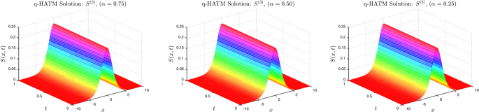
q-HATM \(S^{(3)}\)-solutions with different α when \(\hbar =-1\), \(\mathcal{A}=r=0.1\), \(\mathcal{B}=3\), and \(n=1\) for Example 4.3
-
2.
In Figs. 15–17, the nature of q-HATM solution subject to t with different α for Equations (23), (33), and (44) is presented, and their response helps the reader to understand the effect of fractional order. Furthermore, we observe that \(\hbar =-0.99\) and −1 are in the range of convergence of series solution using the horizontal line test in the ħ-curves, and when \(n=2\), we have a large range of values for the optimal choice of ħ.
Figure 15 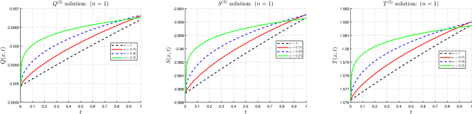
Nature of q-HATM solution with different α when \(\hbar =-1\), \(k=\eta =0.1\), \(r=-1.5\), \(p=1.5\), and \(x=10\) for Example 4.1
Figure 16 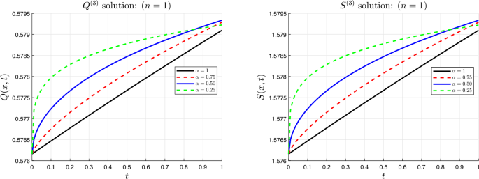
Nature of q-HATM solution with different α when \(\hbar =-1\), \(k=r=0.1\), \(\lambda =1.5\), and \(x=10\) for Example 4.2
Figure 17 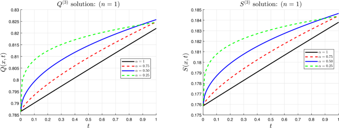
Nature of q-HATM solution with different α when \(\hbar =-1\), \(\mathcal{A}=r=0.1\), \(\mathcal{B}=3\), and \(x=1\) for Example 4.3
Figure 18 
ħ-curves plot with different α when \(k=\eta =0.1\), \(r=-1.5\), \(p=1.5\), \(x=10\), and \(t=0.1\) for Example 4.1
Figure 19 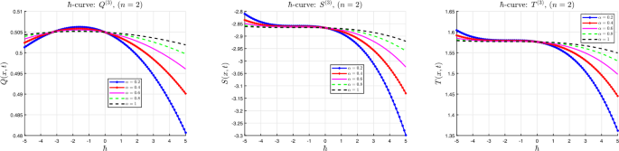
ħ-curves plot with different α when \(k=\eta =0.1\), \(r=-1.5\), \(p=1.5\), \(x=10\), and \(t=0.1\) for Example 4.1
Figure 20 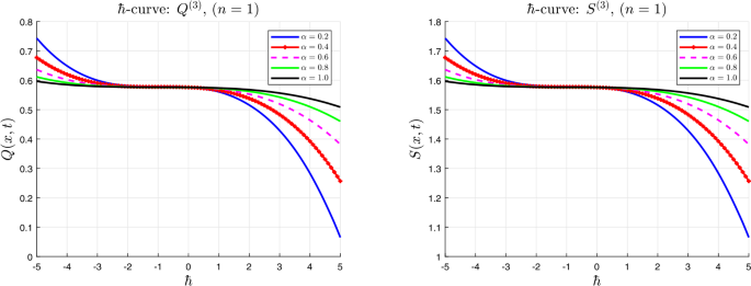
ħ-curves plot with different α when \(k=0.1\), \(\lambda =1.5\), \(x=10\), and \(t=0.1\) for Example 4.2
Figure 21 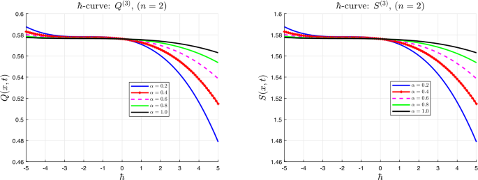
ħ-curves plot with different α when \(k=0.1\), \(\lambda =1.5\), \(x=10\), and \(t=0.1\) for Example 4.2
Figure 22 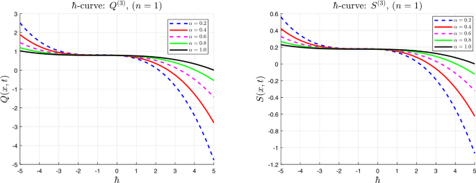
ħ-curves plot with different α when \(r=0.1\), \(\mathcal{B}=3\), \(x=1\), and \(t=0.1\) for Example 4.3
Figure 23 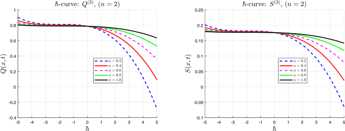
ħ-curves plot with different α when \(r=0.1\), \(\mathcal{B}=3\), \(x=1\), and \(t=0.1\) for Example 4.3


5 Numerical comparison
This section is devoted to comparison of the results presented above with several other analytical methods in the literature such as new iterative method (NIM) in [35, 43], differential transformation method (DTM) and reduced differential transformation method (RDTM) in [40], and homotopy perturbation method (HPM) in [44]. We consider the case where \(\alpha =1\) in order to use exact solution as the benchmark.
6 Conclusion
In this paper, the time-fractional Hirota–Satsuma coupled with KdV, coupled KdV, and modified coupled KdV systems, which describe interactions of two long waves with different dispersion relations, are considered using q-homotopy analysis transformation method. The proposed method presents a series solution in a form of recurrence relation with high accuracy and minimal computations. Several numerical comparisons are made with well-known analytical methods and the exact solutions when \(\alpha =1\). It is evident from Tables 3–10 that the proposed method outperformed other methods in handling the coupled systems considered in this paper. Hence, we can conclude that q-HATM is highly methodical and can be used to investigate strongly nonlinear fractional mathematical models describing natural phenomena. In the future, the authors will look into other numerical methodologies such as fourth-order nonstandard compact finite difference [68] or sixth-order implicit finite difference [69] both of high order difference schemes to solve the above proposed problems.
References
Kumar, D., Seadawy, A.R., Joardar, A.K.: Modified Kudryashov method via new exact solutions for some conformable fractional differential equations arising in mathematical biology. Chin. J. Phys. 56(1), 75–85 (2018)
Baleanu, D., Wu, G.C., Zeng, S.D.: Chaos analysis and asymptotic stability of generalized Caputo fractional differential equations. Chaos Solitons Fractals 102, 99–105 (2017)
Nasrolahpour, H.: A note on fractional electrodynamics. Commun. Nonlinear Sci. Numer. Simul. 18, 2589–2593 (2013)
Hilfer, R., Anton, L.: Fractional master equations and fractal time random walks. Phys. Rev. E 51, R848–R851 (1995)
Zhang, Y., Pu, Y.F., Hu, J.R., Zhou, J.L.: A class of fractional-order variational image in-painting models. Appl. Math. Inf. Sci. 6(2), 299–306 (2012)
Pu, Y.F.: Fractional differential analysis for texture of digital image. J. Algorithms Comput. Technol. 1(3), 357–380 (2007)
Baleanu, D., Guvenc, Z.B., Machado, J.T.: New Trends in Nanotechnology and Fractional Calculus Applications. Springer, Berlin (2010)
Mainardi, F.: Fractional Calculus and Waves in Linear Viscoelasticity. Imperial College Press, London (2010)
Salahshour, S., Ahmadian, A., Senu, N., Baleanu, D., Agarwal, P.: On analytical solutions of the fractional differential equation with uncertainty: application to the Basset problem. Entropy 17, 885–902 (2015)
Ruzhansky, M.V., Je Cho, Y., Agarwal, P., Area, I.: Advances in Real and Complex Analysis with Applications. Springer, Singapore (2017)
Saoudi, K., Agarwal, P., Kumam, P., Ghanmi, A., Thounthong, P.: The Nehari manifold for a boundary value problem involving Riemann–Liouville fractional derivative. Adv. Differ. Equ. 2018, 263 (2018)
Jain, S., Agarwal, P., Kilicman, A.: Pathway fractional integral operator associated with 3m-parametric Mittag-Leffler functions. Int. J. Appl. Comput. Math. 4(5), 115 (2018)
Agarwal, P., Dragomir, S.S., Jleli, M., Samet, B.: Advances in Mathematical Inequalities and Applications. Springer, Berlin (2018)
El-Sayed, A.A., Agarwal, P.: Numerical solution of multiterm variable order fractional differential equations via shifted Legendre polynomials. Math. Methods Appl. Sci. 42, 3978–3991 (2019)
Qureshi, S., Yusuf, A.: Mathematical modeling for the impacts of deforestation on wildlife species using Caputo differential operator. Chaos Solitons Fractals 126, 32–40 (2019)
Nigmatullina, R.R., Agarwal, P.: Direct evaluation of the desired correlations: verification on real data. Phys. A, Stat. Mech. Appl. 534, 121558 (2019)
Rekhviashvili, S., Pskhu, A., Agarwal, P., Jain, S.: Application of the fractional oscillator model to describe damped vibrations. Turk. J. Phys. 43(3), 236–242 (2019)
Qureshi, S., Yusuf, A.: Fractional derivatives applied to MSEIR problems: comparative study with real world data. Eur. Phys. J. Plus 134(4), 171 (2019)
Jajarmi, A., Arshad, S., Baleanu, D.: A new fractional modelling and control strategy for the outbreak of dengue fever. Phys. A, Stat. Mech. Appl. 535, 122524 (2019)
Yıldız, T.A., Jajarmi, A., Yıldız, B., Baleanu, D.: New aspects of time fractional optimal control problems within operators with nonsingular kernel. Discrete Contin. Dyn. Syst. 13(3), 407–428 (2020)
Yusuf, A., Qureshi, S., Shah, S.F.: Mathematical analysis for an autonomous financial dynamical system via classical and modern fractional operators. Chaos Solitons Fractals 132, 109552 (2020)
Jajarmi, A., Yusuf, A., Baleanu, D., Inc, M.: A new fractional HRSV model and its optimal control: a non-singular operator approach. Phys. A, Stat. Mech. Appl. 547, 123860 (2020). https://doi.org/10.1016/j.physa.2019.123860
Jain, S., Mehrez, K., Baleanu, D., Agarwal, P.: Certain Hermite–Hadamard inequalities for logarithmically convex functions with applications. Mathematics 7(2), 163 (2019)
Baleanu, D., Jajarmi, A., Sajjadi, S.S., Mozyrska, D.: A new fractional model and optimal control of a tumor-immune surveillance with non-singular derivative operator. Chaos, Interdiscip. J. Nonlinear Sci. 29(8), 083127 (2019)
Jajarmi, A., Baleanu, D., Sajjadi, S.S., Asad, J.H.: A new feature of the fractional Euler–Lagrange equations for a coupled oscillator using a nonsingular operator approach. Front. Phys. 7, 196 (2019)
Jajarmi, A., Ghanbari, B., Baleanu, D.: A new and efficient numerical method for the fractional modelling and optimal control of diabetes and tuberculosis co-existence. Chaos, Interdiscip. J. Nonlinear Sci. 29(9), 093111 (2019)
Caputo, M.: Elasticita e Dissipazione. Zanichelli, Bologna (1969)
Liao, S.J.: Homotopy analysis method: a new analytic method for nonlinear problems. Appl. Math. Mech. 19, 957–962 (1998)
Podlubny, I.: Fractional Differential Equations. Academic Press, New York (1999)
Miller, K.S., Ross, B.: An Introduction to Fractional Calculus and Fractional Differential Equations. Wiley, New York (1993)
Hirota, R., Satsuma, J.: Soliton solutions of a coupled Korteweg–de Vries equation. Phys. Lett. A 85, 407–418 (1981)
Wu, Y.T., Geng, X.G., Hu, X.B., Zhu, S.M.: Generalized Hirota–Satsuma coupled Korteweg–de Vries equation and Miura transformations. Phys. Lett. A 64, 255–259 (1999)
Korteweg, D.J., de Vries, G.: XLI. On the change of form of long waves advancing in a rectangular canal, and on a new type of long stationary waves. Philos. Mag. 39(240), 422–443 (1895)
Wu, Y., Geng, X., Hu, X., Zhu, S.: A generalized Hirota–Satsuma coupled Korteweg–de Vries equation and Miura transformations. Phys. Lett. A 255(4–6), 259–264 (1999)
Sontakke, B.R., Shaikh, A., Nisar, K.S.: Approximate solutions of a generalized Hirota–Satsuma coupled KdV and a coupled mKdV systems with time fractional derivatives. Malaysian J. Math. Sci. 12(2), 175–196 (2018)
Ganji, D.D., Rafei, M.: Solitary wave solutions for a generalized Hirota–Satsuma coupled KdV equations by homotopy perturbation method. Phys. Lett. A 356, 131–137 (2006)
Kaya, D.: Solitary wave solutions for a generalized Hirota–Satsuma coupled KdV equations. Appl. Math. Comput. 147, 69–78 (2004)
Abbasbandy, S.: The application of homotopy analysis method to solve a generalized Hirota–Satsuma coupled KdV equation. Phys. Lett. A 361, 478–483 (2007)
Guo-Zhong, Z., Xi-Jun, Y., Yun, X., Jiang, Z., Di, W.: Approximate analytic solutions for a generalized Hirota Satsuma coupled KdV equation and a coupled mKdV equation. Chin. Phys. B 19, 080204 (2010)
Abazari, R., Abazari, M.: Numerical simulation of generalized Hirota–Satsuma coupled KdV equation by RDTM and comparison with DTM. Commun. Nonlinear Sci. Numer. Simul. 17, 619–629 (2012)
Fan, E.G.: Soliton solutions for a generalized Hirota–Satsuma coupled KdV equation and a coupled MKdV equation. Phys. Lett. A 282(1–2), 18–22 (2001)
Arife, A.S., Karimi Vanani, S., Yildirim, A.: Numerical solution of Hirota–Satsuma couple KdZ and a coupled MKdV equation by means of homotopy analysis method. World Appl. Sci. J. 13(11), 2271–2276 (2011)
Jibran, M., Nawaz, R., Khan, A., Afzal, S.: Iterative solutions of Hirota Satsuma coupled KDV and modified coupled KDV systems. Math. Probl. Eng. 2018, Article ID 9042039 (2018)
Ganji, Z.Z., Ganji, D.D., Rostamiyan, Y.: Solitary wave solutions for a time-fraction generalized Hirota–Satsuma coupled KdV equation by an analytical technique. Appl. Math. Model. 33, 3107–3113 (2009)
Ghoreishi, M., Ismail, A.I., Rashid, A.: The solution of coupled modified KdV system by the homotopy analysis method. TWMS J. Pure Appl. Math. 3(1), 122–134 (2012)
Kaya, D., Inan, I.E.: Exact and numerical travelling wave solutions for nonlinear coupled equations using symbolic computation. Appl. Math. Comput. 151, 775–787 (2004)
Liao, S.J.: Homotopy analysis method and its applications in mathematics. J. Basic Sci. Eng. 5(2), 111–125 (1997)
El-Tawil, M.A., Huseen, S.N.: The Q-homotopy analysis method (QHAM). Int. J. Appl. Math. Mech. 8(15), 51–75 (2012)
Akinyemi, L., Iyiola, O.S., Akpan, U.: Iterative methods for solving fourth- and sixth-order time-fractional Cahn–Hillard equation. Math. Methods Appl. Sci. 43(7), 4050–4074 (2020). https://doi.org/10.1002/mma.6173
Akinyemi, L.: q-homotopy analysis method for solving the seventh-order time-fractional Lax’s Korteweg–de Vries and Sawada–Kotera equations. Comput. Appl. Math. 38(4), 191 (2019)
Şenol, M., Iyiola, O.S., Daei Kasmaei, H., Akinyemi, L.: Efficient analytical techniques for solving time-fractional nonlinear coupled Jaulent–Miodek system with energy-dependent Schrödinger potential. Adv. Differ. Equ. 2019, 462 (2019)
Iyiola, O.S.: On the solutions of non-linear time-fractional gas dynamic equations: an analytical approach. Int. J. Pure Appl. Math. 98(4), 491–502 (2015)
Iyiola, O.S., Soh, M.E., Enyi, C.D.: Generalised homotopy analysis method (q-HAM) for solving foam drainage equation of time fractional type. Math. Eng. Sci. Aerosp. 4(4), 105 (2013)
Iyiola, O.S.: A numerical study of Ito equation and Sawada–Kotera equation both of time-fractional type. Adv. Math. Sci. J. 2(2), 71–79 (2013)
Soh, M.E., Enyi, C.D., Iyiola, O.S., Audu, J.D.: Approximate analytical solutions of strongly nonlinear fractional BBM-Burger’s equations with dissipative term. Appl. Math. Sci. 8(155), 7715–7726 (2014)
Singh, J., Kumar, D., Swroop, R.: Numerical solution of time and space-fractional coupled Burgers’ equations via homotopy algorithm. Alex. Eng. J. 55(2), 1753–1763 (2016)
Kumar, D., Agarwal, R.P., Singh, J.: A modified numerical scheme and convergence analysis for fractional model of Lienard’s equation. J. Comput. Appl. Math. 399, 405–413 (2018)
Prakash, A., Veeresha, P., Prakasha, D.G., Goyal, M.: A homotopy technique for fractional order multi-dimensional telegraph equation via Laplace transform. Eur. Phys. J. Plus 134, 19 (2019)
Singh, J., Kumar, D., Baleanu, D., Rathore, S.: An efficient numerical algorithm for the fractional Drinfeld–Sokolov–Wilson equation. Appl. Math. Comput. 335, 12–24 (2018)
Srivastava, H.M., Kumar, D., Singh, J.: An efficient analytical technique for fractional model of vibration equation. Appl. Math. Model. 45, 192–204 (2017)
Kumara, D., Singha, J., Baleanu, D.: A new analysis for fractional model of regularized long-wave equation arising in ion acoustic plasma waves. Math. Methods Appl. Sci. 40, 5642–5653 (2017)
Veeresha, P., Prakasha, D.G., Qurashi, M.A., Baleanu, D.: A reliable technique for fractional modified Boussinesq and approximate long wave equations. Adv. Differ. Equ. 2019, 253 (2019)
Dhaigude, C.D., Nikam, V.R.: Solution of fractional partial differential equations using iterative method. Fract. Calc. Appl. Anal. 15(4), 684–699 (2012)
Luchko, Y.F., Srivastava, H.M.: The exact solution of certain differential equations of fractional order by using operational calculus. Comput. Math. Appl. 29, 73–85 (1995)
Kilbas, A.A., Srivastava, H.M., Trujillo, J.J.: Theory and Applications of Fractional Differential Equations. North-Holland Mathematics Studies, vol. 204. Elsevier, Amsterdam (2006)
Odibat, Z.M., Shawagfeh, N.T.: Generalized Taylor’s formula. Appl. Math. Comput. 186(1), 286–293 (2007)
Argyros, I.K.: Convergence and Applications of Newton-Type Iterations. Springer, New York (2008)
Hajipour, M., Jajarmi, A., Baleanu, D.: On the accurate discretization of a highly nonlinear boundary value problem. Numer. Algorithms 79(3), 679–695 (2018)
Hajipour, M., Jajarmi, A., Malek, A., Baleanu, D.: Positivity-preserving sixth-order implicit finite difference weighted essentially non-oscillatory scheme for the nonlinear heat equation. Appl. Math. Comput. 325, 146–158 (2018)
Acknowledgements
The authors thank the referees for a number of suggestions which have improved many aspects of this article.
Availability of data and materials
Not applicable.
Funding
No funding available for this project.
Author information
Authors and Affiliations
Contributions
The authors read and approved the final manuscript.
Corresponding author
Ethics declarations
Competing interests
The authors declare to have no competing interests.
Rights and permissions
Open Access This article is licensed under a Creative Commons Attribution 4.0 International License, which permits use, sharing, adaptation, distribution and reproduction in any medium or format, as long as you give appropriate credit to the original author(s) and the source, provide a link to the Creative Commons licence, and indicate if changes were made. The images or other third party material in this article are included in the article’s Creative Commons licence, unless indicated otherwise in a credit line to the material. If material is not included in the article’s Creative Commons licence and your intended use is not permitted by statutory regulation or exceeds the permitted use, you will need to obtain permission directly from the copyright holder. To view a copy of this licence, visit http://creativecommons.org/licenses/by/4.0/.
About this article

Cite this article
Akinyemi, L., Iyiola, O.S. A reliable technique to study nonlinear time-fractional coupled Korteweg–de Vries equations. Adv Differ Equ 2020, 169 (2020). https://doi.org/10.1186/s13662-020-02625-w
Received:
Accepted:
Published:
DOI: https://doi.org/10.1186/s13662-020-02625-w