The q-cosine Fourier transform and the q-heat equation

Abstract

The aim of this work is to establish in great detail The q-Fourier analysis related to the q-cosine. The wise reader will note that the considered q-cosine coincides with the one given by T.H. Koornwinder and S.F. Swarttouw. Through the q-cosine product formula, we define and analyze the properties of the q-even translation and the q-convolution. Adopting the Titchmarsh approach, we study the q-cosine Fourier transform and its inverse formula.

The second theme of this paper is an application of the q-Fourier analysis developed earlier. We extend the heat representation theory inaugurated by P.C. Rosenbloom and D.V. Widder to the q-analogue. We construct the q-solution source, the q-heat polynomials and solve the q-analytic Cauchy problem.

1 Introduction

During the last years, an intensive work was founded about the so-called q-basic theory. Taking account of the well-known Ramanujan works shown at the beginning of this century by Jackson ([9, 10]), many authors such as Askey, Gasper, Ismail, Rogers, Andrew, Koornwinder, and others (see references) have recently developed this topic.

The present article is devoted to the study of the q-analogue of the Fourier transforms and to showing how it plays a central role in solving the q-heat equation associated to the second q-derivative operator. The method used here differs from those given by T.H. Koornwinder and R.F. Swarttouw, who discovered a q-analogue of Hankel’s Fourier–Bessel via some q-analogue orthogonality relations. We note that Ph. Feinsilver [4] gave a q-Harmonic Analysis for a q-Laplace transform with inversion formula.

Without entering into a dilemma through the analysis presented here, it seems that the point of view of T.H. Koornwinder and R.F. Swarttouw [12] is more suitable for harmonic analysis. We take as definition of the q-cosine the one given by the previous authors with a simple change and we prefer to write it as a series of functions denoted as b _n (x;q ²). This q-cosine appears as an eigenfunction of the operator Δ _q . Owing to a nice paper [12], we give a product formula written with the q-Jackson integral and we study the q-translation and the q-convolution. Next we define the q-analogue of the cosine Fourier transform with the purpose to find the transformation inverse. To this end, we prove the equivalent of the so-called Riemann–Lebesgue Lemma and discover that the Titchmarsh approach holds [15].

A motivation behind this work is to state some result about the q-heat equation associated to Δ _q operator. We attempt to extend the heat representation theory studied in many cases ([5, 7, 14], etc.). We define the q-heat polynomials and find that they are linked to the q-Hermite polynomials [13] and constitute with the q-associated functions a biorthogonal system. We conclude by solving the q-analytic Cauchy problem related to the q-heat equation.

2 Notations and preliminaries

We begin by recalling some q-elements of quantum analysis adapting the notation used in the book of Gasper and Rahman [6]. Let a and q be real numbers such that 0<q<1, the q-shift factorial is defined by

$$ (a;q)_{0}=1,\qquad (a;q)_{n}={\prod_{k=0}^{n-1}} \bigl(1-aq^{k} \bigr),\quad n=1,2,\ldots ,\infty. $$

(1)

A basic hypergeometric series is

$${}_{r}\varphi_{s}(a_{1},\ldots ,a_{r};b_{1},\ldots ,b_{s};q,z)=\sum _{k=0}^{\infty}\frac{(a_{1},\ldots ,a_{r};q)_{k}}{(b_{1},\ldots ,b_{s},q;q)_{k}} \bigl[ (-1)^{k}q^{\binom{k}{2}} \bigr]^{1+s-r}z^{k}. $$

A function f is q-regular at zero if lim _n→∞ f(xq ⁿ)=f(0) exists and is independent of x.

The q-derivative D _q f of a function f is defined by

$$ D_{q}f(x)=\frac{f(x)-f(qx)}{(1-q)x},\quad x\neq0. $$

(2)

The q-derivative at zero is defined by

$$D_{q}f ( 0 ) =\lim_{n\rightarrow\infty}\frac{f ( xq^{n} ) -f ( 0 ) }{xq^{n}}, $$

if it exists and does not depend on x.

We introduce the set

$$\mathbb{R}_{q}= \bigl\{q^{k};k\in\mathbb{Z} \bigr\}.$$

The q-integral of Jackson is defined by

The q-integration by parts is given for suitable functions f and g by

$$ {\int_{0}^{\infty}} f(x)D_{q}g(x)\,d_{q}x= \bigl[ f(x)g(x) \bigr]_{0}^{\infty}-{\int _{0}^{\infty}} f(x)D_{q}g \bigl(q^{-1}x \bigr)\,d_{q}x. $$

(3)

The q-analogue of the Gamma function is defined as

$$ \varGamma_{q}(x)=\frac{(q;q)_{\infty}}{(q^{x};q)_{\infty}}(1-q)^{1-x}, $$

(4)

which tends to Γ(x) when q tends to 1⁻.

3 q-Trigonometric functions

We define the q-cosine as

$$ \cos \bigl(x;q^{2} \bigr)={_{1}\phi_{1}} \bigl(0;q;q^{2},(1-q)^{2}x^{2} \bigr)=\sum _{n=0}^{\infty }(-1)^{n}b_{n} \bigl(x;q^{2} \bigr), $$

(5)

where we have put

$$ b_{n} \bigl(x;q^{2} \bigr)=b_{n} \bigl(1;q^{2} \bigr)x^{2n}=q^{n(n-1)} \frac{(1-q)^{2n}}{(q;q)_{2n}}x^{2n}. $$

(6)

In the same way, the q-sine is given by

$$\sin \bigl(x;q^{2} \bigr)= ( 1-q ) x{_{1} \phi_{1}} \bigl(0;q^{3};q^{2},(1-q)^{2}x^{2} \bigr)=\sum_{n=0}^{\infty}(-1)^{n}c_{n} \bigl(x;q^{2} \bigr), $$

with

$$c_{n} \bigl(x;q^{2} \bigr)=c_{n} \bigl(1;q^{2} \bigr)x^{2n+1}=\frac{q^{n(n-1)}(1-q)^{2n+1}}{(q;q)_{2n+1}}x^{2n+1}. $$

These q-trigonometric functions differ and should not be confused with the functions cos _q and sin _q considered in [6, p. 23]; but coincide with the one given in [12] and [15] with a minor change of variable. Furthermore, we have

Proposition 3.1

The following statements hold:

• 1.
  $$b_{n} \bigl(0,q^{2} \bigr)=\delta_{n,0},\qquad \varDelta_{q}b_{n} \bigl(x;q^{2} \bigr)=b_{n-1}\bigl(x;q^{2} \bigr),\quad n\geq1; $$
• 2.
  $$\bigl \vert b_{n} \bigl(x;q^{2} \bigr) \bigr \vert \leq \frac{x^{2n}}{ ( 2n ) !}, $$

where

$$ \varDelta_{q}u ( x ) = \bigl( D_{q}^{2}u \bigr) \bigl( q^{-1}x \bigr) . $$

(7)

Proof

We only prove Part 2 since Part 1 is deduced from the definition of Δ _q .

The coefficients b _n (1;q ²), defined by (6), can be written as

where we have put q=e ^−t, t>0.

Since the functions

$$f(t)=\frac{e^{-jt}-e^{-(j+1)t}}{1-e^{-(j+1)t}}\quad \mbox{and}\quad g(t)=\frac {e^{-jt}-e^{-(j+1)t}}{1-e^{-(2j+2)t}}, $$

decrease on ]0,∞[, we obtain

$$b_{n} \bigl(1;q^{2} \bigr)\leq{\frac{1}{{(2n)!}}}. $$

 □

As a consequence of the previous proposition, we can show that for λ∈ℂ the function

$$\cos \bigl(\lambda x;q^{2} \bigr)=\sum_{0}^{\infty}(-1)^{n}b_{n} \bigl(x;q^{2} \bigr){\lambda}^{2n},$$

is the unique analytic solution of the q-differential equation

$$ \varDelta_{q}u(x)=-{\lambda}^{2}u(x), $$

(8)

with

$$ u(0,q)=1,\qquad ( D_{q}u ) ( 0 ) =0. $$

(9)

Proposition 3.2

For x∈ℝ _q and $\frac{\operatorname{Log}(1-q)}{\operatorname{Log}(q)}\in\mathbb{Z}$, we have

• 1.
  $$\bigl \vert \cos \bigl(x,q^{2} \bigr) \bigr \vert \leq \frac{1}{(q;q^{2})_{\infty}^{2}}; $$
• 2.
  $$\lim_{x\rightarrow\infty}\cos \bigl(x,q^{2} \bigr)=0; $$
• 3.
  $$\bigl \vert \sin \bigl(x,q^{2} \bigr) \bigr \vert \leq \frac{1}{(q;q^{2})_{\infty}^{2}}; $$
• 4.
  $$\lim _{x\rightarrow\infty}\sin \bigl(x,q^{2} \bigr)=0. $$

Proof

To prove Parts 1 and 2, we use the properties of ₁ ϕ ₁ given in [12] and their connection to the q-cosine. We obtain

$$ \bigl|\cos \bigl(q^{1+n};q^{2} \bigr)\bigr|\leq{\frac{1}{{(q;q^{2})_{\infty}^{2}}}}\left\{\begin{array}{l@{\quad }l} 1& \mbox{if}\ n\geq0,\\ q^{n^{2}} & \mbox{if}\ n\leq0. \end{array}\right.$$

(10)

hence Parts 1 and 2 follow. A similar argument shows Parts 3 and 4. □

Now we try to find a product formula for the q-cosine functions. We begin by proving the following result.

Proposition 3.3

For reals x and y, y≠0, we have

(11)

Note that this formula can be expressed in terms of ₁ φ ₁ as follows

(12)

Proof

To show (11) and (12), we begin by expanding the q-cosines in series absolutely and uniformly convergent on every compact of ℝ. From the product rule of series and the fact that

$$\frac{1}{(q;q)_{2n-2k}}=\frac{(q^{2n-2k+1},q)_{\infty}}{(q;q)_{\infty}}=0,\quad k>n, $$

we obtain for y≠0

$$\cos \bigl(x;q^{2} \bigr)\cos \bigl(y;q^{2} \bigr)=\sum _{k=0}^{\infty}{\frac{q^{2k^{2}}}{{(q;q)_{2k}}}} \biggl({ \frac{x}{y}} \biggr)^{2k}\sum_{n=0}^{\infty}(-1)^{n} \frac{q^{n^{2}-n}}{(q;q)_{2n-2k}}q^{-2nk}y^{2n}. $$

On the other hand, we have

$$\frac{1}{(q;q)_{2n-2k}}=\frac{q^{-k(2k-1)+2nk}}{(q;q)_{2n}}{ \sum _{s=-k}^{s=k}} ( -1 )^{k-s}\frac{q^{\binom{k-s}{2}}}{ ( q;q )_{k-s} ( q;q )_{k+s}}q^{2ns}.$$

We deduce (11) after the interchange of summation order. To prove (12), we write

$$\cos \bigl(x;q^{2} \bigr)\cos \bigl(y;q^{2} \bigr)=I+J, $$

with

$$I=\sum_{s=0}^{\infty}\cos \bigl(q^{s}y;q^{2} \bigr)\sum_{k\geq s}q^{k} \biggl( \frac{x}{y}\biggr)^{2k}\frac{(-1)^{k-s}q^{\frac{(k-s)(k-s-1)}{2}}}{(q;q)_{k+s}(q;q)_{k-s}},$$

$$J=\sum_{s=-\infty}^{-1}\cos \bigl(q^{s}y;q^{2} \bigr)\sum_{k\geq-s}q^{k} \biggl( \frac{x}{y}\biggr)^{2k}\frac{(-1)^{k-s}q^{\frac{(k-s)(k-s-1)}{2}}}{(q;q)_{k-s}(q;q)_{k+s}}.$$

In I, we make the change k−s into k and use the equality

$$(q;q)_{k+2s}=(q;q)_{2s} \bigl(q^{1+2s};q \bigr)_{k}, $$

to obtain

$$I=\sum_{s=0}^{\infty}q^{s} \biggl({ \frac{x}{y}} \biggr)^{2s}\frac{(q^{2s+1};q)_{\infty}}{(q;q)_{\infty}}{_{1} \phi_{1}} \bigl(0;q^{1+2s};q,q \bigl(q^{2}/y^{2} \bigr) \bigr)\cos \bigl(q^{s}y;q^{2} \bigr). $$

Now we make the change k+s into k in J and use the equalities

$$(q;q)_{k-2s}=(q;q)_{-2s} \bigl(q^{1-2s};q \bigr)_{k},\quad -s\geq1, $$

$${\frac{(k-2s)(k-2s-1)}{2}}={\frac{(k-2)(k-3)}{2}}-2sk+2s^{2}-1, $$

and

This identity is easily deduced from [11]. Then we obtain

$$J=\sum_{s=-\infty}^{-1}q^{s} \bigl(x^{2}/y^{2} \bigr)^{2s}\frac{(q^{1+2s};q)_{\infty}}{(q;q)_{\infty}}{_{1} \phi_{1}} \bigl(0;q^{1+2s};q,qx^{2}/y^{2} \bigr)\cos \bigl(q^{s}y;q^{2} \bigr). $$

We add these sums to find that (12) holds. □

Remark 3.4

(1) If we replace y by q ^y, x by q ^x, and assume the proposition the hypothesis, we obtain from (12) that the following integral representation holds

(2) The product formula (11) leads to

$$ \cos \bigl(x;q^{2} \bigr)\cos \bigl(y;q^{2} \bigr)=\sum _{n=0}^{\infty}b_{n} \bigl(x;q^{2} \bigr) \varDelta_{q}^{n}\cos \bigl( y;q^{2} \bigr) . $$

(13)

4 q-Translation and q-convolution

We define, for x and y in ℝ _q , the measure

$$ d_{q}\mu_{(x,y)}=\sum_{s=-\infty}^{\infty} \mathcal{{D}} \bigl(x,y;q^{s} \bigr)q^{s}\delta_{yq^{s}}, $$

(14)

where δ _u denotes the unit mass supported at u, and

$$ \mathcal{{D}} \bigl(x,y;q^{s} \bigr)= \biggl({\frac{x}{y}} \biggr)^{2s}\frac{(q({\frac{x}{y}})^{2};q)_{\infty}}{(q;q)_{\infty}}{_{1}\phi_{1}} \biggl(0;q \biggl({\frac{x}{y}}\biggr)^{2};q,q^{1+2s} \biggr). $$

(15)

Proposition 4.1

(1) For x and y in ℝ _q , we have

$$d_{q}\mu_{ ( x,y ) }=d_{q}\mu_{ ( y,x ) }. $$

(2) d _q μ _(x,y) is of bounded variation.

(3)

$${\int} d_{q} \mu_{ ( x,y ) }(t)=1. $$

Proof

For n,m∈ℤ, the relation (2.3) from [12] leads to

$$\mathcal{{D}} \bigl(q^{n},q^{m};q^{s} \bigr)= \mathcal{{D}} \bigl(q^{m},q^{n};q^{s+m-n} \bigr). $$

We obtain Part 1 after the change s−n+m by s.

To prove Part 2, we suppose $|{\frac{x}{y}}|\leq1$; from the formulas (2.4) in [12] we have

$$ |d_{q}\mu_{(x,y)}|_{var}\leq \biggl( \frac{|y|^{2}+q|x|^{2}}{|y|^{2}-q|x|^{2}}\biggr)\frac{(q|{\frac{x}{y}}|^{2};-q,q)_{\infty}}{(q,q)_{\infty}}. $$

(16)

Finally, from (2.8) in [12], we can show that Part 3 is true. □

We introduce the q-translation which generalizes the even translation given by ${\frac{1}{2}}(\delta_{x+y}+\delta_{x-y})$.

Let f be a function with support in ℝ _q , the q-translation is defined for x and y in ℝ _q by

$$ T_{x,q}f(y)=\int_{0}^{\infty}f(t)\,d_{q} \mu_{(x,y)}(t). $$

(17)

From the previous proposition and the q-product formula (12), we have

Proposition 4.2

Let f be a function with compact support in ℝ _q . We have

• (i)
  $$T_{q,y}\cos \bigl( x;q^{2} \bigr) =\cos \bigl( x;q^{2} \bigr) \cos \bigl( y;q^{2} \bigr) . $$
• (ii)
  
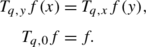
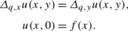
• (iii)
  

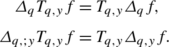
• (iv) The function u(x,y)=T _q,y f(x) is a solution of the problem

  

From the relation

$$\varDelta_{q}^{n}(f) ( x ) =\frac{q^{(2-n)n} ( q;q )_{2n}}{ ( 1-q )^{2n}}{\sum_{k=-n}^{n}} ( -1 )^{n-k} \frac{q^{\binom{n-k}{2}}}{ ( q;q )_{n-k} ( q;q )_{n+k}}f \bigl( q^{k}x \bigr) , $$

we can write the q-translation of a function f as

$$ T_{q,y}f ( x ) ={\sum _{n=0}^{\infty}} b_{n} \bigl(y,q^{2} \bigr)\varDelta_{q,x}^{n}f ( x ) , $$

(18)

and have in the limit when q tends to 1⁻ the classical even translation cited before.

Now we denote by $L_{q}^{1}(\mathbb{R}_{q})$ the space of functions f defined on ℝ _q such that

$$\Vert f\Vert _{1,q}=\int_{-\infty}^{\infty}\bigl|f(t)\bigr|\,d_{q}t< \infty. $$

Then we are able to define the q-convolution by

$$ f\star_{q}g(x)=\frac{(1+q^{-1})^{1/2}}{\varGamma_{q^{2}}(1/2)}\int_{0}^{\infty }T_{x,q}f(y)g(y)\,d_{q}y, $$

(19)

where f and g are two functions in $L_{q}^{1}(\mathbb{R}_{q})$. We can show that this space is an algebra.

5 q-Analogue of Fourier-cosine

In this section, we suppose $\frac{\operatorname{Log}(1-q)}{\operatorname{Log}(q)}\in\mathbb{Z}$. The q-analogue of Fourier transform is defined for λ∈ℝ _q by

$$ \mathcal{F}(f) (\lambda)={\frac{(1+q^{-1})^{1/2}}{\varGamma_{q^{2}}(1/2)}}\int_{0}^{\infty}f(t) \cos \bigl(\lambda t;q^{2} \bigr)\,d_{q}t, $$

(20)

where f is a function in $L_{q}^{1}(\mathbb{R}_{q})$.

This definition is the same (after a minor change) as that given by T.H. Koornwinder and R.F. Swarttouw (see [12]).

Proposition 5.1

For $f, g\in L_{q}^{1}(\mathbb{R}_{q})$, the following properties hold:

• (1)
  $$ \bigl \vert \mathcal{F}_{q} ( f ) ( \lambda ) \bigr \vert \leq \frac{1}{ [ q ( 1-q ) ]^{\frac{1}{2} } ( q;q )_{\infty}} \Vert f\Vert_{1,q},\quad \lambda\in\mathbb{R}_{q}; $$

  (21)
• (2)
  $$ \mathcal{F}_{q} ( \mathcal{T}_{q,x}f ) ( \lambda ) =\cos \bigl(\lambda x;q^{2} \bigr)\mathcal{F}_{q} ( f ) ( \lambda ) ,\quad \lambda\in\mathbb{R}_{q};$$

  (22)
• (3)
  $$\mathcal{F}_{q}(f\star_{q}g)=\mathcal{F}_{q}(f) \mathcal{F}_{q}(g). $$

Proof

Part 1. The inequality (21) follows from Proposition 3.2 and the identity

$$\bigl(q;q^{2} \bigr)_{\infty} \bigl(q^{2};q^{2} \bigr)_{\infty}=(q;q)_{\infty}. $$

Part 2 is a direct consequence of the q-product formula (12).

Part 3 is obtained after the exchange of the integration order and taking into account the invariability of the q-integral by the q-translation. □

Now we focus our attention on the inversion of the linear map $\mathcal{F}_{q}$. We proceed by looking at the q-analogue of the Riemman–Lebesgue Lemma, the localization theorem, and we show that the Titchmarsh approach holds in the q-theory.

Proposition 5.2

Let f be a function in $L_{q}^{1} ( \mathbb{R}_{q} )$, then

$$\lim_{\lambda\longrightarrow\infty}\mathcal{F}_{q} ( f ) (\lambda)=0,\quad \lambda\in\mathbb{R}_{q}. $$

Proof

To prove this, first we have from Proposition 3.2

$$\bigl \vert f(x)\cos \bigl(\lambda x;q^{2} \bigr) \bigr \vert \leq \frac{1}{(q;q^{2})_{\infty}^{2}} \bigl \vert f(x) \bigr \vert \in L_{q}^{1} ( \mathbb{R}_{q} ) ,\quad x,\lambda\in\mathbb{R}_{q}. $$

And for λ∈ℝ _q we have

$$\lim _{\lambda\rightarrow\infty}f(x)\cos \bigl(\lambda x;q^{2} \bigr)=0,\quad \lambda \in\mathbb{R}_{q}, $$

so the result is true. □

Proposition 5.3

We have the identity

$$\int_{0}^{\infty}\frac{\sin ( x;q^{2} ) }{x}\,d_{q}x= \frac {\varGamma_{q^{2}}^{2} ( \frac{1}{2} ) }{1+q^{-1}}. $$

Proof

This is a consequence of (2.8) in [12]. □

Proposition 5.4

Let f:(0,∞)→ℂ satisfy the conditions:

• (1) $f\in L_{q}^{1} ( \mathbb{R}_{q} )$,

• (2) For a∈ℝ _q , there exists C(a)>0 such that

  $$\bigl \vert f \bigl( aq^{k} \bigr) -f ( 0 ) \bigr \vert \leq C ( a ) q^{k},\quad k=0,1,2,\ldots . $$

Then

$$\lim _{\lambda\rightarrow+\infty}\int_{0}^{\infty}f ( x ) \frac{\sin ( \lambda x;q^{2} ) }{x}\,d_{q}x=\frac{\varGamma_{q^{2}}^{2} ( \frac{1}{2} ) }{1+q^{-1}}f ( 0 ) . $$

Proof

Indeed, the first hypothesis shows that for an arbitrary ε>0 we have for large q ^−N,N=0,1,… , that

$$\int_{q^{-N}}^{\infty} \biggl \vert \frac{f ( x ) }{x} \biggr \vert \,d_{q}x\leq\frac{\varepsilon}{2} \bigl(q;q^{2} \bigr)_{\infty}^{2}$$

and

The second hypothesis and Proposition 3.2 show that

$$\biggl \vert \frac{f ( q^{k-N} ) -f ( 0 ) }{q^{k-N}}\sin \bigl( \lambda q^{k-N};q^{2} \bigr) \biggr \vert \leq\frac{C ( N ) }{q^{-N} ( q,q^{2} )_{\infty}^{2}}. $$

Since from Proposition 3.2 we have that sin(λx;q ²) tends to zero as λ tends to ∞, the proposition is then a direct consequence. □

Theorem 5.5

(The q-cosine Fourier integral theorem)

If $f\in L_{q}^{1} ( \mathbb{R}_{q} )$ is such that for a∈ℝ _q there exist positive constants C(a) such that

$$ \bigl|T_{x,q}f \bigl(aq^{k} \bigr)-f \bigl(q^{k} \bigr)\bigr| \leq C(a)q^{k},\quad k=0,1,\ldots, $$

(23)

then

(24)

6 q-Heat equation and q-heat polynomials

In this section, the two q-analogues of the elementary exponential functions are crucial and they are defined by

(25)

and

$$ e \bigl(x;q^{2} \bigr)=\frac{1}{((1-q^{2})x;q^{2})_{\infty}}=\sum _{0}^{\infty}\frac{(1-q^{2})^{n}}{(q^{2};q^{2})_{n}}x^{n}, \quad |x|<\frac{1}{1-q^{2}}. $$

(26)

These functions satisfy the identity

$$e \bigl(x;q^{2} \bigr)E \bigl(-x;q^{2} \bigr)=1, $$

and have as limit, when q tends to 1⁻, the classical exponential function.

Now we purpose to give the q-analogue of the heat equation associated to the second derivative operator (even in x)

$$ \frac{\delta^{2}u}{\delta x^{2}}=\frac{\delta u}{\delta t},\quad x\in \mathbb{R},\ t>0. $$

(27)

We consider as q-heat equation associated to the second q-derivative operator the partial q-difference equation

$$ (\varDelta_{q,x}u) (x,t)=(D_{q^{2},t}u) (x,t). $$

(28)

We take as the initial condition

$$ u(x,0)=f(x),\quad f\in L_{q}^{1} ( \mathbb{R}_{q} ) . $$

(29)

6.1 q-Solution source

To find the solution source related to the q-heat equation, we apply the Fourier method with the adapted q-Fourier cosine studied before.

Putting

$$U(\lambda,t)=\mathcal{{F}} \bigl(u(x,t) \bigr) (\lambda), $$

Eq. (28) becomes

$$D_{q^{2},t}U(\lambda,qt)=-{\lambda}^{2}U(\lambda,t), $$

and, taking into account conditions (29), we obtain

$$U(\lambda,t)=\mathcal{{F}}(f) (\lambda)e \bigl(-{\lambda}^{2}t;q^{2} \bigr). $$

The problem consists in finding the function which has e(−λ ² t;q ²) as its q-Fourier-cosine transform. For this end, we need the following lemma.

Lemma 6.1

For n=0,1,2,… and t>0, we have

Proof

From (26) we find

$$\int _{0}^{\infty}e \biggl(-\frac{\lambda^{2}}{qt(1+q)^{2}},q^{2} \biggr)\lambda^{2n}\,d_{q}\lambda=(1-q)\sum_{-\infty}^{\infty}\frac{q^{ ( 2n+1 ) k}}{ ( -\frac{1-q}{1+q}\frac{q^{2k}}{qt},q^{2} )_{\infty}}\mathtt{.}$$

Secondly, the use of the well-known Ramanujan [8] identity

$$\sum _{-\infty}^{\infty} \frac{z^{k}}{ ( bq^{k},q )_{\infty }}=\frac{ ( bz,q/bz,q,q )_{\infty}}{ ( b,z,q/b,q )_{\infty}},\quad b\neq0, $$

leads to the result after minor computation. □

Proposition 6.2

$$\frac{ ( 1+q^{-1} )^{1/2}}{\varGamma_{q^{2}} ( 1/2 ) }{\int_{0}^{\infty}} e \biggl(-\frac{\lambda^{2}}{qt(1+q)^{2}},q^{2} \biggr)\cos \bigl( \lambda x,q^{2} \bigr)\,d_{q}\lambda=A \bigl( t,q^{2} \bigr) e \bigl( -tx^{2},q^{2} \bigr), $$

where

$$ A \bigl( t,q^{2} \bigr) = \bigl[ (1-q)q^{-1} \bigr]^{1/2}\frac{ ( -\frac{1+q}{1-q}q^{2}t,-\frac{1-q}{1+q}\frac{1}{t},q^{2} )_{\infty}}{ ( -\frac{1-q}{1+q}\frac{1}{qt},-\frac{1+q}{1-q}q^{3}t;q^{2} )_{\infty}}. $$

(30)

As an immediate consequence we are now able to define the q-source solution associated to the q-heat equation (28) by

$$ G \bigl(x,t,q^{2} \bigr)= \bigl(A \bigl( t,q^{2} \bigr) \bigr)^{-1}e \biggl(-\frac{x^{2}}{qt(1+q)^{2}};q^{2} \biggr). $$

(31)

In the same manner as in the classical heat equation theory, we put

$$ G \bigl(x,y,t;q^{2} \bigr)=T_{y,q}G \bigl(x,t;q^{2} \bigr), $$

(32)

with T _y,q being the q-translation studied in Sect. 4.

Through this approach we show that the solution of the q-Cauchy problem (28) and (29) can been written in the form of

$$ u(x,t)= \bigl(G \bigl(\cdot,t;q^{2} \bigr)\star_{q}f \bigr) (x)=\int_{0}^{\infty}G \bigl(x,y,t;q^{2} \bigr)f(y)\,d_{q}y. $$

(33)

It is natural to ask how other properties such as the positivity of G(x,t;q ²) and the existence of the q-semigroup can be established.

6.2 q-Heat polynomials

Proposition 6.3

It is easy to see that, for x∈ℝ and t>0, the analytic function

$$\lambda\rightarrow e{ \bigl(-{\lambda}^{2}t;q^{2} \bigr)\cos \bigl(\lambda x;q^{2} \bigr)}, $$

is a solution of (28) and it has the expansion

$$e \bigl( -\lambda^{2}t,q^{2} \bigr) \cos \bigl(\lambda x,q^{2} \bigr)=\sum _{n=0}^{\infty} ( -1 )^{n}v_{2n}(x,t,q)\lambda^{2n},$$

where

$$ v_{2n}(x,t,q)=\sum _{k=0}^{n}b_{k} \bigl( x,q^{2} \bigr) \frac {(1-q^{2})^{n-k}}{(q^{2};q^{2})_{n-k}}t^{n-k}, $$

(34)

with the functions b _n being given by (6).

From Proposition 3.1 we deduce immediately the following properties:

We note that formula (34) can be inverted:

$$ b_{n} \bigl(x;q^{2} \bigr)=\sum _{k=0}^{n}(-1)^{n-k}v_{2k}(x,t;q)q^{ ( n-k ) ( n-k-1 ) } \frac{(1-q^{2})^{n-k}}{(q^{2};q^{2})_{n-k}}t^{n-k}. $$

(35)

Proposition 6.4

The q-heat polynomials (34) possess the q-integral representation

• (1)
  $$ v_{2n}(x,t;q)={\int _{0}^{\infty}} G \bigl(x,y,t,q^{2} \bigr)b_{n} \bigl(y;q^{2} \bigr)\,d_{q}y. $$

  (36)
• (2)
  $$ b_{n} \bigl(x;q^{2} \bigr)={\int_{0}^{\infty}} G \bigl(x,y,t,q^{2} \bigr)v_{2n} \bigl(q^{-1/2}y,t;q^{-1} \bigr)\,d_{q}y. $$

  (37)

Proof

We have

and

 □

In [14], the authors defined the so-called associated functions by the Appell transform. We extend this notion by defining for t>0 the q-associated functions of v _2n by

$$ w_{2n}(x,t;q)= ( -1 )^{n} \varDelta_{q,y}^{n}G \bigl(x,y,t;q^{2}\bigr) \bigl\vert_{y=0}. $$

(38)

It is easy to see that

$$ w_{2n}(x,t;q)=\frac{ ( 1+q^{-1} )^{1/2}}{\varGamma_{q^{2}} ( 1/2 ) }{ \int_{0}^{\infty}} e \bigl(-t \lambda^{2},q^{2} \bigr)\lambda^{2n}\cos \bigl( \lambda x,q^{2} \bigr)\,d_{q}\lambda. $$

(39)

Proposition 6.5

(Biorthogonality)

For t>0 and n,m∈ℕ, we have

$${\int_{0}^{\infty}} w_{2m}(x,t;q)v_{2n} \bigl(q^{1/2}x,-t;q \bigr)\,d_{q}x= ( -1 )^{m}\delta_{n,m}. $$

Proof

By (37), we have

$$\varDelta_{q}^{m}b_{n} \bigl(x;q^{2} \bigr)={\int_{0}^{\infty}} \varDelta_{q}^{m}G \bigl(x,y,t,q^{2} \bigr)v_{2n} \bigl(q^{-1/2}y,t;q^{-1} \bigr)\,d_{q}y. $$

Putting x=0, we obtain

$${\int_{0}^{\infty}} w_{2m}(y,t;q)v_{2n} \bigl(q^{-1/2}y,t;q^{-1} \bigr)\,d_{q}y= ( -1 )^{m}\delta_{n,m}. $$

 □

6.3 Convergence of ∑ _n≥0 α _n v _2n (x,t;q)

Now we establish the following estimates that will be needed later

Lemma 6.6

For n=0,1,… and $0< \frac{x_{0}^{2}}{t_{0}} <+\infty$, we have

$$\bigl| v_{2n}(x_{0},t_{0},q)\bigr| \geq \frac{(1-q^{2})^{n}}{(q^{2};q^{2})_{n}}\vert t_{0}\vert ^{n}\geq \frac{\vert t_{0}\vert ^{n}}{n!}. $$

Proof

Indeed, the first inequality is a consequence of b ₀(1;q ²)=1 and the hypothesis, and the second follows from

$$\frac{1}{n!}\leq\frac{(1-q^{2})^{n}}{(q^{2};q^{2})_{n}}. $$

 □

Corollary 6.7

For n=0,1,… and $0 < \frac{x_{0}^{2}}{t_{0}}< +\infty$, we have

$$\big| v_{2n}(x_{0},t_{0},q)\big| \geq Cn^{-\frac{1}{2}} \biggl( \frac{\vert t_{0}\vert e}{n} \biggr)^{n}, $$

where C is a constant depending on x ₀ and t ₀.

Lemma 6.8

For n=0,1,…,δ>0, and $\vert \frac{x^{2}}{\delta ( 1+q ) }\vert <1$, we have

$$ \frac{(1-q^{2})^{n}}{(q^{2};q^{2})_{n}}\bigl| v_{2n} \bigl(\vert x\vert ,\vert t\vert ,q \bigr)\bigr| \leq q^{-n ( n-1 ) }\frac{ ( \delta+\vert t\vert )^{n}}{n!}e \biggl( \frac{x^{2}}{\delta ( 1+q ) };q \biggr) . $$

(40)

Proof

To show (40), we note that

$$(q;q)_{2k}= \bigl(q,q^{2};q^{2} \bigr)_{k},$$

and

$$\bigl(q;q^{2} \bigr)_{k}\geq(q;q)_{k}. $$

For δ>0, and by using the fact that

$$\frac{(1-q)^{k}}{(q;q)_{k}}\frac{|x|^{2}}{(\delta(1+q))^{k}}\leq q^{-\binom {k}{2}}\exp \biggl( \frac{\vert x\vert ^{2}}{\delta(1+q)} \biggr), $$

we obtain

The inequalities

$$\biggl(-\frac{|t|}{\delta};q^{2} \biggr)_{n}\leq \biggl( \frac{|t|}{\delta}+1 \biggr)^{n}, $$

and

$$q^{\binom{n}{2}}n!\leq\frac{ ( q;q )_{n}}{ ( 1-q )^{n}}\leq n! , $$

give the result. □

By the Stirling formula, we obtain

Corollary 6.9

For n=0,1,…,δ>0, and $\vert \frac{x^{2}}{\delta ( 1+q ) }\vert <1$, we have

$$ v_{2n} \bigl(\vert x\vert ,\vert t\vert ,q \bigr)\leq K q^{-n ( n-1 ) } \biggl( \bigl( \delta+\vert t\vert \bigr) \frac{n}{e} \biggr)^{n}, $$

(41)

where K is a constant depending δ.

Theorem 6.10

Let (α _n ) be a sequence of real or complex numbers such that

$$\overline{\lim_{n\rightarrow\infty}} {\frac{n}{e}}q^{-2(n-1)}| \alpha_{n}|^{1/n}={\frac{1}{\sigma}}<+\infty. $$

Then the series

$$\sum_{n\geq0}\alpha_{n}v_{2n}(x,t;q), $$

converges in the strip

$$ S_{\sigma}= \bigl\{(x,t),x\in\mathbb{R},\ |t|<\sigma \bigr\}, $$

(42)

and converges uniformly in any region of this strip.

To prove the theorem, we adopt the same approach as in [14] by taking account of the q-equivalent estimation (41).

Remark

If we write u(x,t) as the sum of the previous series, then this function satisfies the q-heat equation (28) and

$$u(x,0)=\sum_{n=0}^{\infty}\alpha_{n}b_{n} \bigl(x;q^{2} \bigr), $$

where the b _n (x;q ²) is given by (6).

6.4 Analytic Cauchy problem related to the q-heat equation

Lemma 6.11

Under the hypothesis of Theorem 6.10 and putting

$$ u ( x,t ) =\sum_{n\geq0}\alpha_{n}v_{2n}(x,t;q), $$

(43)

u(x;t) is an analytic function of two variables x and t in the strip S _σ given by (42) and satisfies the q-heat equation (28). Furthermore, the coefficients α _n are given by

$$ \alpha_{n}= \varDelta_{q}^{n}u ( x,t ) \bigl\vert_{ ( x,t ) = ( 0,0 ) }. $$

(44)

Proof

To show this, we note that the theorem gives that u(x,t) is analytic in the whole strip S _σ . Now for a fixed integer p the series

$$\sum_{n\geq0}\alpha_{n+p}v_{2n}(x,t;q) $$

converges uniformly in any compact region of S _σ . To prove (44), it suffices to see that for integers n and p we have

$$\bigl(\varDelta_{q,x}^{n}v_{2p}(x,t;q)\bigr)\bigl|_{(0,0)}= \delta_{n,p}, $$

where δ _n,p is the Kronecker symbol. □

Finally the following statement is established.

Theorem 6.12

Under the hypothesis of Lemma 6.11, the function u(x,t) given by (43) has the q-Maclaurin expansion

$$u(x,t)=\sum_{m,p\geq0}\beta_{m,p} \frac{(1-q^{2})^{m}}{(q^{2};q^{2})_{m}}x^{2p}t^{m}, $$

where

$$ \beta_{m,p}=\alpha_{m+p}b_{p} \bigl( 1,q^{2} \bigr) . $$

(45)

If for x∈ℝ and |t|<σ then function

$$u(x,t)=\sum_{m,p}\beta_{m,p} \frac{(1-q^{2})^{m}}{(q^{2};q^{2})_{m}}x^{2p}t^{m}, $$

satisfies the q-heat equation (28) with the coefficients β _m,p given by (44), then u(x,t) can be extended to an analytic function in the strip S _σ and we have

$$u(x,t)=\sum_{n\geq0}\alpha_{n}v_{2n}(x,t;q). $$

References

Andrews, G.E.: q-Series: Their Development and Application in Analysis, Number Theory, Combinatorics, Physics, and Computer Algebra. Regional Conference Series in Math., vol. 66. Amer. Math. Soc., Providence (1986)
Askey, R., Ismail, M.E.H.: A Generalization of Ultraspherical Polynomials. In: Erdos, P. (ed.) Studies in Pure Mathematics. Birkhäuser, Basel (1983)
Baley, W.N.: Generalized Hypergeometric Series. Cambridge University Press, Cambridge (1935). Reprinted by Hafner Publishing Company (1972)
Feinsilver, Ph.: Elements of q-harmonic analysis. J. Math. Anal. Appl. 141, 509–526 (1989)
Fitouhi, A.: Heat “polynomials” for a singular differential operator on (0,∞). Constr. Approx. 5, 241–270 (1989)
Gasper, G., Rahman, M.: Basic Hypergeometric Series. Encyclopedia of Mathematics and Its Applications, vol. 35. Cambridge University Press, Cambridge (1990)
Haimo, D.T.: Expansion of generalized heat polynomials and their appell transform. J. Math. Mech. 15, 735–758 (1966)
Ismail, M.E.H.: A simple proof of Ramanujan’s 1 ψ 1 sum. Proc. Am. Math. Soc. 63, 185–186 (1977)
Jackson, F.H.: On q-Functions and a Certain Difference Operator. Transactions of the Royal Society of London, vol. 46, pp. 253–281 (1908)
Jackson, F.H.: On a q-definite integrals. Q. J. Pure Appl. Math. 41, 193–203 (1910)
Koornwinder, T.H.: q-Special functions, a tutorial, Mathematical preprint series, Report 94-08, Univer. Amsterdam, The Netherlands
Koornwinder, T.H., Swarttouw, R.F.: On q-analogues of the Hankel and Fourier transform. Trans. Am. Math. Soc. 333, 445–461 (1992)
Moak, D.S.: The q-analogue of the Laguerre polynomials. J. Math. Anal. Appl. 81, 21–47 (1981)
Rosenbloom, P.C., Widder, D.V.: Expansions in terms of heat polynomials and associated functions. Trans. Amer. Math. Soc. 92, 220–266 (1959)
Swarttouw, R.F.: The Hahn–Exton q-Bessel function, Thesis
Titchmarsh, E.C.: Introduction to The Theory of Fourier Integrals, 2nd edn. Oxford University Press, Oxford (1937)
Open Access
This article is distributed under the terms of the Creative Commons Attribution License which permits any use, distribution, and reproduction in any medium, provided the original author(s) and the source are credited.
Author information
Authors and Affiliations
Corresponding author
Additional information
This research is supported by NPST Program of King Saud University, project number 10-MAT1293-02.
EDITORIAL NOTE: The article was accepted on 16 February, 2001, before the papers of the Ramanujan Journal were handled electronically. Unfortunately this article in its printed form was misplaced. The delay caused in publication is regretted.
Rights and permissions
Open Access This article is distributed under the terms of the Creative Commons Attribution 2.0 International License (https://creativecommons.org/licenses/by/2.0), which permits unrestricted use, distribution, and reproduction in any medium, provided the original work is properly cited.
About this article
Cite this article
Fitouhi, A., Bouzeffour, F. The q-cosine Fourier transform and the q-heat equation. Ramanujan J 28, 443–461 (2012). https://doi.org/10.1007/s11139-012-9412-8
Received:
Accepted:
Published:
Issue Date:
DOI: https://doi.org/10.1007/s11139-012-9412-8