
Abstract
We propose a new modification of homotopy perturbation method (HPM) called the δ-homotopy perturbation transform method (δ-HPTM). This modification consists of the Laplace transform method, HPM, and a control parameter δ. This control convergence parameter δ in this new modification helps in adjusting and controlling the convergence region of the series solution and overcome some limitations of HPM and HPTM. The δ-HPTM and q-homotopy analysis transform method (q-HATM) are considered to study the generalized time-fractional perturbed \((3+1)\)-dimensional Zakharov–Kuznetsov equation with Caputo fractional time derivative. This equation describes nonlinear dust-ion-acoustic waves in the magnetized two-ion-temperature dusty plasmas. The selection of an appropriate value of δ in δ-HPTM and the auxiliary parameters n and ħ in q-HATM gives a guaranteed convergence of series solution, but the difference between the two techniques is that the embedding parameter p in δ-HPTM varies from zero to nonzero δ, whereas the embedding parameter q in q-HATM varies from zero to \(\frac{1}{n}, n\geq{1}\). We examine the effect of fractional order on the considered problem and present the error estimate when compared with exact solution. The outcomes reveal complete reliability and efficiency of the proposed algorithm for solving various types of physical models arising in sciences and engineering. Furthermore, we present the convergence and error analysis of the two methods.
1 Introduction
The study of fractional partial differential equations (FPDEs) has enticed the interest of many researchers in the field of applied sciences and engineering by virtue of its enormous applications in electrodynamics, random walk, biotechnology, viscoelasticity, chaos theory, signal and image processing, nanotechnology, and many other areas [1–20]. Also, essential properties of fractional calculus were outlined by many researchers (see [21–24] for detailed discussion). Nevertheless, solving FPDEs is generally more complex than the classical type since their operators are defined through integrals. There are many techniques proposed by many researchers to handle analytical and approximate solutions of nonlinear FPDEs such as the residual power series method [25–28], iterative Shehu transform method [29], Laplace decomposition method [30], q-homotopy analysis method [31–34], Adomian decomposition method [35], fractional reduced differential transform method [36, 37], variational iteration method [38, 39], homotopy analysis method [40], and other methods [41–44].
The homotopy perturbation method (HPM) was developed by He [45–50] by combining the perturbation and standard homotopy for solving numerous physical problems. We refer the reader to He’s works for a clear understanding of HPM, where further insights can be found. Recently, an improved modification of HPM, called the parameterized homotopy perturbation method (PHPM), was proposed in [51, 52]. Another formulation, called the He–Laplace method, was proposed to obtain an exact closed approximate solution of nonlinear models [53, 54]. The HPM and well-known Laplace transformation method were combined to produce a highly effective technique, called the homotopy perturbation transform method (HPTM), for solving many nonlinear problems [55, 56]. It is worth noting that the Laplace transform method alone in some cases is insufficient in handling nonlinear problems because of the difficulties that may arise by the nonlinear terms. In this present study, we propose a new modification of HPM, called the δ-homotopy perturbation transform method (δ-HPTM), which consists of HPM, the Laplace transform method, and a control parameter δ. Similarly to the control parameters n and ħ in q-HATM, the control parameter δ in δ-HPTM also helps in adjusting and controlling the convergence region of the series solutions and can overcome some limitations of HPM, HPTM, and He–Laplace method. It is worth mentioning that the present modification (δ-HPTM) requires neither polynomials like ADM nor Lagrange multipliers like VIM and overcomes the limitations of these methods.
To elucidate the reliability and effectiveness of the proposed modification, we consider the generalized time-fractional perturbed \((3+1)\)-dimensional Zakharov–Kuznetsov (gpZK) equation given by
where W represents the electrostatic potential, k is a positive number, γ is the fractional order, ξ represents a smallness parameter, and the physical quantities \(\beta_{1}, \beta_{2}\), and \(\beta_{3}\) are constants. Zhen et al. [57] and Seadawy et al. [58, 59] have outlined these physical quantities. This equation is used to describe the nonlinear dust-ion-acoustic waves in the magnetized two-ion-temperature dusty plasmas [60, 61]. The study of ion-acoustic waves and structures in dense quantum plasmas has attracted a lot of consideration in recent years. The ZK equation comprises the nonlinear term \(W\frac{\partial{W}}{\partial{x}}\) and third-order dispersion term \(\frac{\partial^{3} W}{\partial{x^{3}}}\):
Equation (2) is limited to the waves of small amplitudes only. The width of the soliton and its velocity deviate from the predictions of this equation as the amplitude of the wave increases. The pZK equation (1) with fractional order \(\gamma=1\) and \(k=1\) includes an of extra fifth-order dispersion term \(\xi\frac{\partial^{5} W}{\partial x^{5}}\) was proposed to overcome this problem (see [57–59, 62], for more detail). The proposed δ-HPTM and q-HATM are employed to compute numerical solutions of Eq. (1). The two algorithms provide the solutions in a rapid convergent series, which can lead the solutions to a closed form. To the author’s knowledge, the approximate solutions of the gpZK (1) was not addressed in the literature before.
The rest of the paper is structured as follows. Useful notations and definitions are provided in Sect. 2. The essential idea of the two methods with convergence and error analysis are presented in Sect. 3. The applications of δ-HPTM and q-HATM on the generalized time-fractional pZK equation are detailed in Sect. 4. Numerical comparison and discussion are provided in Sect. 5. Lastly, Sect. 6 concludes the paper.
2 Preliminaries
This section contains some helpful notations and definitions.
Definition 1
Let \(\omega\in\mathbb{R}\) and \(m\in\mathbb{N}\). A function W is said to be in the space \(\mathbb{C}_{\omega}\) if there exists \(\eta\in\mathbb{R}\), \(\eta>\omega\), and \(Z\in C{[0, \infty)}\) such that \(W(t)=t^{\eta}Z(t)\) \(t\in\mathbb{R}^{+}\). Furthermore, \(W\in\mathbb{C}^{m}_{\omega}\) if \(W^{(m)}\in\mathbb{C}_{\omega}\) [63].
Definition 2
The Riemann–Liouville (RL) fractional integral of order γ of a function \(W(t)\in C_{\omega}, \omega\geq{-1}\), is given as [23, 63–65]
where \(J^{0}W(t)=W(t)\), and Γ is the classical gamma function.
Definition 3
The fractional derivative of \(W(t)\) (denoted by \(\mathcal{D}^{\gamma}W(t)\)) in the Caputo sense for \(m-1<\gamma<m\), \(m\in\mathbb{N}\), is defined as [23, 65]
where
with the following properties:
-
a.
\(\mathcal{D}^{\gamma} (\tau_{1}W(t)+\tau_{2}V(t) )=\tau_{1} \mathcal{D}^{\gamma}W(t)+\tau_{2} \mathcal{D}^{\gamma}V(t)\), \(\tau_{1},\tau_{2}\in\mathbb{R}\),
-
b.
\(\mathcal{D}^{\gamma}J^{\gamma}W(t)=W(t)\),
-
c.
\(J^{\gamma}\mathcal{D}^{\gamma}W(t)=W(t)-\sum_{j=0}^{m-1}W^{j}_{0}(t) \frac{t^{j}}{j!}\).
Definition 4
The Laplace transform (denoted by \(\mathscr{L}\)) of a Riemann–Liouville fractional integral \((J_{t}^{\gamma}W(t) )\) and Caputo fractional derivative \((\mathcal{D}_{t}^{\gamma}W(t) )\) of a function \(W\in\mathbb{C}_{\omega} (\omega\geq{-1})\) are given respectively as [21, 65]
where s is a parameter.
3 Analysis of the proposed methods
Here we give the general idea of the δ-HPTM and q-HATM. We also present some convergence and error analysis of the two methods. Consider the general nonlinear FPDE of the form
with initial conditions
where \(\mathcal{D}_{t}^{\gamma}\) represents the Caputo fractional derivative, \(\mathcal{M}\) and \(\mathcal{N}\) denote, respectively, the linear and nonlinear differential operators, \(W=W(x,y,z,t)\) specifies the unknown function, and \(\Phi=\Phi(x,y,z,t)\) is the provided source term. Applying the Laplace transform (denoted by \(\mathscr{L}\)) to both sides of Eq. (7), we have
Using the differentiation property of the Laplace transform with the initial conditions (8), upon simplification and the inverse Laplace transform (denoted by \(\mathscr{L}^{-1}\)), we obtain
3.1 The δ-homotopy perturbation transform method (δ-HPTM)
We employ the concept of HPM [45–50] to Eq. (10) as follows:
We decompose the nonlinear term as
where \(\mathcal{H}_{r}(W)\) are the He’s polynomials expressed in the form
In view of δ-HPM [66], we derive the propose δ-HPTM as
By equating the identical power terms of p in Eq. (14), we generate the sequence of δ-HPTM as
The solution of Eq. (7) is given as
Remark 1
The particular case where \(\delta=1\) is the standard HPTM [55, 56].
3.1.1 Convergence and error analysis
Theorem 1
Let \(W=W(x,y,z,t)\) be defined in a Banach space \(\mathcal{B}\) [67]. Then the series solution
is convergent for a prescribed value of δ if
where \(0<\varrho<\vert\delta\vert\).
Proof
Let \(W_{0}=\mathcal{W}_{0}\in\mathcal{B}\). Define the sequence of partial sums \(\{S_{r}\}\) of Eq. (16) as
We need to show that \(\{S_{r}\}_{r=0}^{\infty}\) is a Cauchy sequence in the Banach space \(\mathcal{B}\). For \(\delta\neq{0}\), we have
For all \(r,k\in\mathbb{N}\) with \(r\geq{k}\), applying the triangle inequality, we obtain
Since \(0<\varrho<\vert\delta\vert\) and \(\delta\neq{0}\), we have \(1- (\frac{\varrho}{\vert\delta\vert} )^{r-k}<1\). Then
Since \(\Vert\mathcal{W}_{0}\Vert<\infty\), we have
Therefore \(\{S_{r}\}_{r=0}^{\infty}\) is a Cauchy sequence in the Banach space \(\mathcal{B}\), so the series solution Eq. (16) converges. □
Theorem 2
If the truncated series \(\sum_{r=0}^{K}\mathcal{W}_{r}(x,y,z,t;\delta)=\sum_{r=0}^{K} W_{r}\delta^{r}\) is employed as an approximate solution of Eq. (7), then the maximum absolute truncation error is estimated as
Proof
It follows from inequality (21) in Theorem 1. For \(M\geq{K}\), we have
For a prescribed value of \(\delta\neq{0}\), \(S_{M}\to W\) as \(M\to\infty\), and \(1- (\frac{\varrho}{\vert\delta\vert} )^{M-K}<1\) (since \(0<\frac{\varrho}{\vert\delta\vert}<1\)). Thus
where \(\mathcal{W}_{0}=W_{0}\). □
3.2 The q-homotopy analysis transform method (q-HATM)
To exemplify the idea of q-HATM [68–75], we construct the zeroth-order deformation equation for \(0\leq q \leq\frac{1}{n}, n\geq{1}\), as
where \(\phi=\phi(x,y,z,t;q)\), and \(\mathcal{N} [\phi ]\) from Eq. (9) is defined as
where q indicates the embedded parameter, the nonzero ħ represents an auxiliary parameter, and \(\mathcal{H}\neq0\) is an auxiliary function. From Eq. (27) with \(q=0, \frac{1}{n}\) we get
As q rises from 0 to \(\frac{1}{n}\), the solutions ϕ ranges from the initial guess \(W_{0}\) to the solution W. In case that \(W_{0}\), ħ, and \(\mathcal{H}\) are all selected appropriately the solutions ϕ in Eq. (27) hold for \(0\leq q \leq\frac{1}{n}\). Hence application of Taylor series expansion [76] to ϕ gives
where
If we choose \(W_{0}\), ħ, and \(\mathcal{H}\) adequately, then Eq. (30) converges at \(q=\frac{1}{n}\). From Eq. (29) we obtain
Differentiating Eq. (27) r times with respect to q, setting \(q=0\), and multiplying by \(\frac{1}{r!}\) give
The vector \(\vec{W}_{r}\) is expressed as
Taking the inverse LT of Eq. (33), we obtain
where
and
In Eq. (36), \(\mathrm{H}_{r}\) denotes the homotopy polynomial defined as
3.2.1 Convergence and error analysis
Here we present some helpful theorems with detailed proofs in [74, 75] for the purpose of completeness.
Theorem 3
(Convergence theorem [74, 75])
Let \(\mathcal{B}\) be a Banach space, and let \(\mathrm{F}:\mathcal{B}\to\mathcal{B}\) be a nonlinear mapping. Suppose that
where \(0<\varrho<1\). Then ϱ has a fixed point in light of Banach’s fixed point theory [77]. Furthermore, for arbitrary choice of \(W_{0},\widehat{W}_{0}\in\mathcal{B}\), the sequence generated by the q-HATM converges to a fixed point of ϱ, and
Theorem 4
([75])
Suppose that the series solution defined in Eq. (32) converges to the solution W for prescribed values of n and ħ and that there is a real number \(0<\Theta<1\) satisfying
If the truncated series
is utilized as an approximation to the solution of problem (7), then the maximum absolute truncated error is evaluated as
4 Application of the proposed methods
We have carefully chosen the generalized time-fractional perturbed \((3+1)\)-dimensional Zakharov–Kuznetsov (gpZK) equation and apply δ-HPTM and q-HATM to obtain analytical approximate solutions in the form of convergent series. Consider
with initial condition
Example 1
Consider Eq. (44) with \(k=1\) given as
with initial condition
where \(e_{0}, p, q\), and ϕ are arbitrary constants. The exact solution for \(\gamma=1\) is given by
δ-HPTM Solution:
Application of δ-HPTM to Eq. (44) with Eq. (45) gives
By equating the identical power terms of p in Eq. (49) we generate the sequence of δ-HPTM as
Hence, using initial condition Eq. (45), we derive:
Accordingly, we can obtain the remaining terms \(W_{r}, r=4, 5, 6, \ldots \) .
q-HATM Solution:
Implementing LT on Eq. (44) with Eq. (45), we obtain
The nonlinear operator \(\mathcal{N}(\phi)\), \(\phi=\phi(x,y,z,t;q)\), is given as
Referring to Eq. (33) with \(\mathcal{H}=1\), the rth-order deformation equation is
where
An application of the inverse LT to Eq. (53) yields
Solving Eqs. (55) using (47) and (54) for \(r=1,2,3,\ldots \) , we get:
Accordingly, we can derive the remaining terms.
Example 2
Consider Eq. (44) with \(k=2\) given as
with initial condition
where \(e_{0}, p, q\), and ϕ are arbitrary constants. The exact solution for \(\gamma=1\) is given by
δ-HPTM Solution:
Application of δ-HPTM to Eq. (56) with Eq. (57) gives
By equating the identical power terms of p in Eq. (59) we generate the sequence of δ-HPTM:
Hence, using initial condition Eq. (57), we derive:
Following this procedure, we can obtain the remaining terms.
q-HATM Solution:
Implementing LT on Eq. (56) with Eq. (57), we obtain
The nonlinear operator \(\mathcal{N}(\phi)\), \(\phi=\phi(x,y,z,t;q)\), is presented as
Referring to Eq. (55), we have
where
Solving Eqs. (64) using (57) and (63) for \(r=1,2,3,\ldots \) , we achieve the following:
Accordingly, we can derive the remaining terms.
Example 3
Consider Eq. (44) with \(k=4\) given as
with initial condition
where p and q are arbitrary constants. The exact solution for \(\gamma=1\) is given by
δ-HPTM Solution
Application of δ-HPTM to Eq. (65) with Eq. (66) gives
By equating the identical power terms of p in Eq. (68) we generate the sequence of δ-HPTM:
Hence, using initial condition Eq. (66), we derive:
By following this procedure we can obtain other terms.
q-HATM Solution:
Implementing LT on Eq. (65) with Eq. (66), we obtain
The nonlinear operator \(\mathcal{N}(\phi)\), \(\phi=\phi(x,y,z,t;q)\), is given as
Referring to Eq. (55), we have
where
Solving Eqs. (73) using (66) and (72) for \(r=1,2,3,\ldots \) , we get:
Respectively, we can derive the remaining terms.
5 Numerical comparison
In this section, the δ-HPTM and q-HATM formulations are tested upon the generalized perturbed \((3+1)\)-dimensional Zakharov–Kuznetsov (gpZK) equation with Caputo fractional derivative. The δ-HPTM solution is presented as
and the q-HATM solution is presented as
We observe that setting \(\delta=\frac{1}{n}\) in Eq. (74) yields
which is the solution of q-HATM. Thus we can conclude that this present modification (δ-HPTM) is more reliable and general. In Figs. 1–6, we present the response of the obtained solutions by the proposed methods with regard to the real and imaginary parts in terms of 2D and 3D plots. The 2D and 3D plots show the graphical comparison of the four-term approximation solutions obtain by δ-HPTM and q-HATM and their exact solutions. The 2D plots also present the effect and behavior of the distinct fractional orders on the solution profile. In addition, Figs. 1–4 exhibit different shapes of the exact and approximate soliton-like solutions, whereas Figs. 5, 6 represent the periodic wave solutions of the gpZK equation. The dynamics of the solution profile can obviously be noted and justify why gpZK should be examined to understand the effects in real-life applications.

The plots of the real part of δ-HPTM, q-HATM, and exact solution for Example 1
The selection of the auxiliary parameters δ in δ-HPTM and ħ in q-HATM are very crucial to guarantee fast convergence of the series solutions. For this reason, in Figs. 7–9, we have provided the so-called δ-curves and ħ-curves of the two proposed methods, which serve as a guide in our optimal selection of values in the present analysis. The horizontal line test is employed to attain the intervals containing optimal values. The comparative study for the case \(\gamma=1\) of the real and imaginary parts of the results obtained by δ-HPTM, q-HATM, and the exact solution as the benchmark are considered in Tables 1–6. From these tables and plots we can observe that the solutions obtained by the proposed methods are very accurate and in agreement with their respective exact solutions.
Remark 2
The parameter values used for Figs. 1–9 are as follows:
-
Figs. 1 and 2: \(\beta_{1}=1, \beta_{2}=2, \beta_{3}=0.1, y=z=2, \xi=0.1, e_{0}=3\), \(p=q=0.5\), \(\phi=1\), \(n=1\), \(\delta=1\), \(\hbar=-1\), and \(t=0.1\).
Figure 2 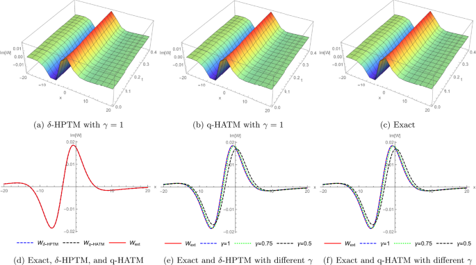
The plots of the imaginary part of δ-HPTM, q-HATM, and exact solution for Example 1
-
Figs. 3 and 4: \(\beta_{1}=1, \beta_{2}=2, \beta_{3}=0.1, y=z=2, \xi=0.1, e_{0}=1, p=q=0.8, \phi=1\), \(n=1\), \(\delta=1, \hbar=-1\), and \(t=0.1\).
Figure 3 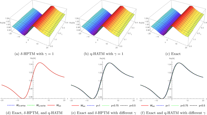
The plots of the real part of δ-HPTM, q-HATM, and exact solution for Example 2
Figure 4 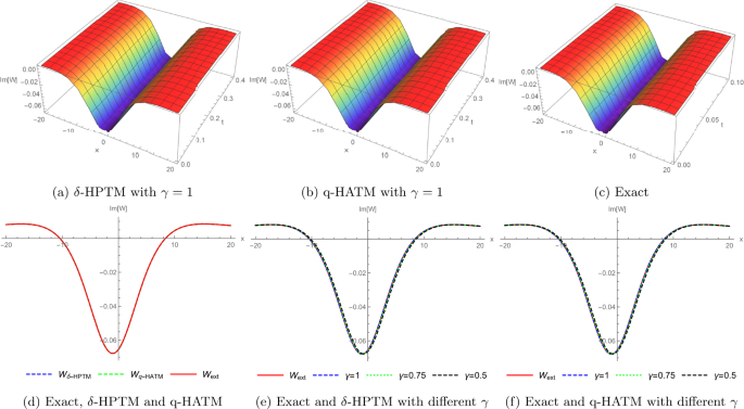
The plots of the imaginary part of δ-HPTM, q-HATM, and exact solution for Example 2
-
Figs. 5 and 6: \(\beta_{1}=1, \beta_{2}=2, \beta_{3}=10, y=z=2, \xi=1, e_{0}=3, p=q=0.3\), \(n=1\), \(\delta=1\), \(\hbar=-1\), and \(t=0.5\).
Figure 5 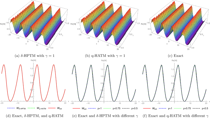
The plots of the real parts of δ-HPTM, q-HATM, and exact solution for Example 3
Figure 6 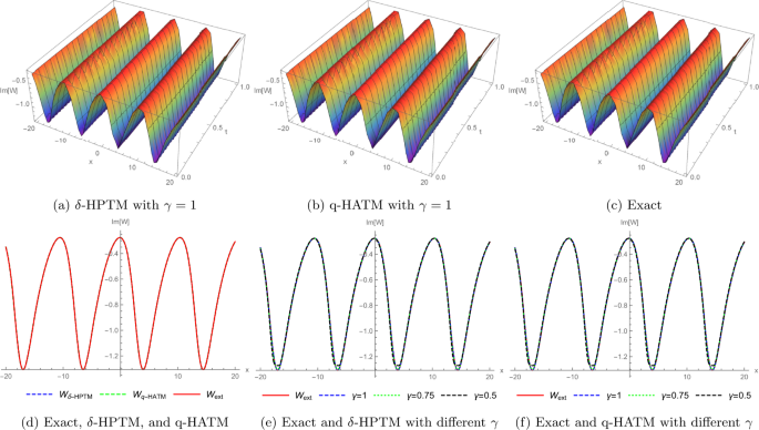
The plots of the imaginary parts of δ-HPTM, q-HATM, and exact solution for Example 3
-
Fig. 7: \(\beta_{1}=1, \beta_{2}=2, \beta_{3}=0.1, \xi=0.1, e_{0}=3, p=0.5, q=0.5, \phi=1, z=y=2, n=1, x=1\), and \(t=0.01\).
Figure 7 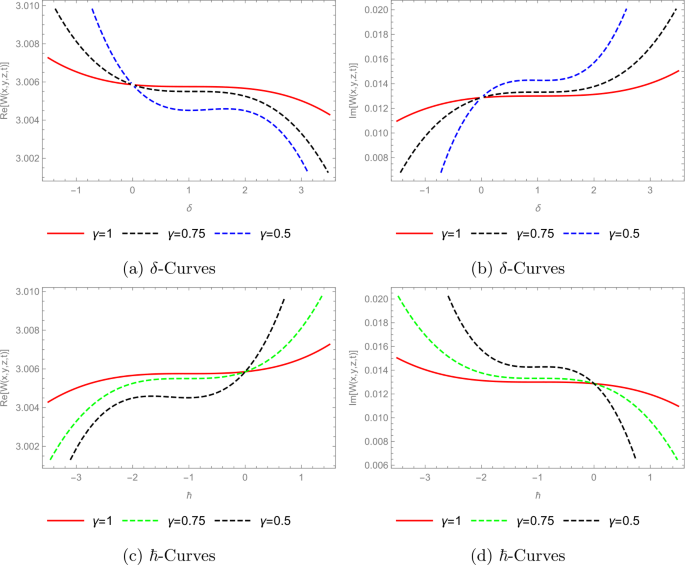
The curves plots of the real and imaginary parts of δ-HPTM and q-HATM solutions for Example 1
-
Fig. 8: \(\beta_{1}=1, \beta_{2}=2, \beta_{3}=0.1, \xi=0.1, e_{0}=1, p=0.8, q=0.8, \phi=1, z=y=2, n=1, x=1\), and \(t=0.01\).
Figure 8 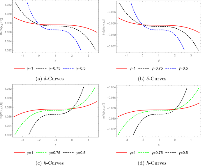
The curves plots of the real and imaginary parts of δ-HPTM and q-HATM solutions for Example 2
-
Fig. 9: \(\beta_{1}=1, \beta_{2}=2, \beta_{3}=10, \xi=1, e_{0}=3, p=0.3, q=0.3, z=y=2, n=1, x=1\), and \(t=0.5\).
Figure 9 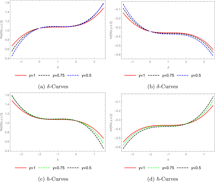
The curves plots of the real and imaginary parts of δ-HPTM and q-HATM solutions for Example 3


6 Conclusion
In this paper, we proposed a new modification of the homotopy perturbation method (HPM), called the δ-homotopy perturbation transform method (δ-HPTM), which consists of HPM, the Laplace transform method, and a control parameter δ for solving integer- and noninteger-order nonlinear problems. We effectively used the proposed method and q-HATM to obtain analytical approximate solutions of the generalized fractional perturbed \((3+1)\)-dimensional Zakharov–Kuznetsov equation. This equation characterizes nonlinear dust-ion-acoustic waves in the magnetized two-ion-temperature dusty plasmas. In comparison to the control parameters n and h in q-HATM, the control parameter δ in δ-HPTM also helps to adjust and control the convergence region of the series solutions and can overcome some limitations of HPM, HPTM, and He–Laplace method. The two methods present series solutions in the form of recurrence relation with high exactness and minimal computations. In reality, we consider HPM, HAM, HPTM, PHPM, and He–Laplace method as particular cases of δ-HPTM and more general when compared with q-HATM (see Eq. (76)). Finally, δ-HPTM can be considered as a good refinement of the existing numerical techniques and can be employed to study strongly nonlinear mathematical models describing natural phenomena.
Availability of data and materials
Not applicable.
References
Owusu-Mensah, I., Akinyemi, L., Oduro, B., Iyiola, O.S.: A fractional order approach to modeling and simulations of the novel COVID-19. Adv. Differ. Equ. 2020(1), 1 (2020). https://doi.org/10.1186/s13662-020-03141-7
Kumar, S., Rashidi, M.M.: New analytical method for gas dynamic equation arising in shock fronts. Comput. Phys. Commun. 185, 1947–1954 (2014)
Kumar, D., Seadawy, A.R., Joardar, A.K.: Modified Kudryashov method via new exact solutions for some conformable fractional differential equations arising in mathematical biology. Chin. J. Phys. 56(1), 75–85 (2018)
Baleanu, D., Wu, G.C., Zeng, S.D.: Chaos analysis and asymptotic stability of generalized Caputo fractional differential equations. Chaos Solitons Fractals 102, 99–105 (2017)
Ghanbari, B., Kumar, S., Kumar, R.: A study of behaviour for immune and tumor cells in immunogenetic tumour model with non-singular fractional derivative. Chaos Solitons Fractals 133, 1–11 (2020). https://doi.org/10.1016/j.chaos.2020.109619
Kumar, S., Kumar, R., Agarwal, R.P., Samet, B.: A study on fractional Lotka Volterra population model by using Haar wavelet and Adams Bashforth–Moulton methods. Math. Methods Appl. Sci. 43(8), 5564–5578 (2020). https://doi.org/10.1002/mma.6297
Kumar, S., Ghosh, S., Samet, B., Goufo, E.F.D.: An analysis for heat equations arises in diffusion process using new Yang–Abdel–Aty–Cattani fractional operator. Math. Methods Appl. Sci. 43(9), 6062–6080 (2020)
Nasrolahpour, H.: A note on fractional electrodynamics. Commun. Nonlinear Sci. Numer. Simul. 18, 2589–2593 (2013)
Hilfer, R., Anton, L.: Fractional master equations and fractal time random walks. Phys. Rev. E 51, R848–R851 (1995)
Zhang, Y., Pu, Y.F., Hu, J.R., Zhou, J.L.: A class of fractional-order variational image in-painting models. Appl. Math. Inf. Sci. 6(2), 299–306 (2012)
Pu, Y.F.: Fractional differential analysis for texture of digital image. J. Algorithms Comput. Technol. 1(3), 357–380 (2007)
Baleanu, D., Guvenc, Z.B., Machado, J.T.: New Trends in Nanotechnology and Fractional Calculus Applications. Springer, Berlin (2010)
Mainardi, F.: Fractional Calculus and Waves in Linear Viscoelasticity. Imperial College Press, London (2010)
Salahshour, S., Ahmadian, A., Senu, N., Baleanu, D., Agarwal, P.: On analytical solutions of the fractional differential equation with uncertainty: application to the Basset problem. Entropy 17, 885–902 (2015)
Ruzhansky, M.V., Je Cho, Y., Agarwal, P., Area, I.: Advances in Real and Complex Analysis with Applications. Springer, Singapore (2017)
Jain, S., Agarwal, P., Kilicman, A.: Pathway fractional integral operator associated with 3m-parametric Mittag-Leffler functions. Int. J. Appl. Comput. Math. 4(5), 115 (2018)
Qureshi, S., Yusuf, A.: Mathematical modeling for the impacts of deforestation on wildlife species using Caputo differential operator. Chaos Solitons Fractals 126, 32–40 (2019)
Nigmatullina, R.R., Agarwal, P.: Direct evaluation of the desired correlations: verification on real data. Phys. A, Stat. Mech. Appl. 534, 121558 (2019)
Rekhviashvili, S., Pskhu, A., Agarwal, P., Jain, S.: Application of the fractional oscillator model to describe damped vibrations. Turk. J. Phys. 43(3), 236–242 (2019)
Qureshi, S., Yusuf, A.: Fractional derivatives applied to MSEIR problems: comparative study with real world data. Eur. Phys. J. Plus 134(4), 171 (2019)
Caputo, M.: Elasticita e Dissipazione. Zanichelli, Bologna (1969)
Liao, S.J.: Homotopy analysis method: a new analytic method for nonlinear problems. Appl. Math. Mech. 19, 957–962 (1998)
Podlubny, I.: Fractional Differential Equations. Academic Press, New York (1999)
Miller, K.S., Ross, B.: An Introduction to Fractional Calculus and Fractional Differential Equations. Wiley, New York (1993)
Zhang, J., Wei, Z., Yong, L., Xiao, Y.: Analytical solution for the time fractional BBM-Burger equation by using modified residual power series method. Complexity 2018, 1–11 (2018). https://doi.org/10.1155/2018/2891373
Alquran, M., Al-Khaled, K., Chattopadhyay, J.: Analytical solutions of fractional population diffusion model: residual power series. Nonlinear Stud. 22(1), 31–39 (2015)
Senol, M., Iyiola, O.S., Daei Kasmaei, H., Akinyemi, L.: Efficient analytical techniques for solving time-fractional nonlinear coupled Jaulent–Miodek system with energy-dependent Schrödinger potential. Adv. Differ. Equ. 2019, 462 (2019)
Senol, M.: Analytical and approximate solutions of \((2+1)\)-dimensional time-fractional Burgers–Kadomtsev–Petviashvili equation. Commun. Theor. Phys. 72, 055003 (2020)
Akinyemi, L., Iyiola, O.S.: Exact and approximate solutions of time-fractional models arising from physics via Shehu transform. Math. Methods Appl. Sci. 1–23 (2020). https://doi.org/10.1002/mma.6484
Khuri, S.A.: A Laplace decomposition algorithm applied to class of nonlinear differential equations. J. Math. Appl. 1(4), 141–155 (2001)
El-Tawil, M.A., Huseen, S.N.: The q-homotopy analysis method (qHAM). Int. J. Appl. Math. Mech. 8, 51–75 (2012)
El-Tawil, M.A., Huseen, S.N.: On convergence of the q-homotopy analysis method. Int. J. Contemp. Math. Sci. 8, 481–497 (2013)
Akinyemi, L., Iyiola, O.S., Akpan, U.: Iterative methods for solving fourth and sixth order time-fractional Cahn–Hillard equation. Math. Methods Appl. Sci. 43(7), 4050–4074 (2020). https://doi.org/10.1002/mma.6173
Akinyemi, L.: q-homotopy analysis method for solving the seventh-order time-fractional Lax’s Korteweg–deVries and Sawada–Kotera equations. Comput. Appl. Math. 38, 1–22 (2019)
Adomian, G.: Solving Frontier Problems of Physics: The Decomposition Method. Kluwer Academic, Norwell (1994)
Keskin, Y., Oturanc, G.: Reduced differential transform method: a new approach to fractional partial differential equations. Nonlinear Sci. Lett. A, Math. Phys. Mech. 1, 61–72 (2010)
Akinyemi, L.: A fractional analysis of Noyes–Field model for the nonlinear Belousov–Zhabotinsky reaction. Comput. Appl. Math. 39, 1–34 (2020). https://doi.org/10.1007/s40314-020-01212-9
He, J.H.: Approximate analytical solution for seepage flow with fractional derivatives in porous media. Comput. Methods Appl. Mech. Eng. 167, 57–68 (1998)
Odibat, Z.M., Momani, S.: Application of variational iteration method to nonlinear differential equations of fractional order. Int. J. Nonlinear Sci. Numer. Simul. 7, 27–34 (2006)
Liao, S.: On the homotopy analysis method for nonlinear problems. Appl. Math. Comput. 147, 499–513 (2004)
Kazem, S., Abbasbandy, S., Kumar, S.: Fractional-order Legendre functions for solving fractional-order differential equations. Appl. Math. Model. 37, 5498–5510 (2013)
Rashidi, M.M., Hosseini, A., Pop, I., Kumar, S., Freidoonimehr, N.: Comparative numerical study of single and two-phase models of nano-fluid heat transfer in wavy channel. Appl. Math. Mech. Engl. 35, 831–848 (2014)
Kumar, S.: A new analytical modeling for telegraph equation via Laplace transform. Appl. Math. Model. 38, 3154–3163 (2014)
Kumar, S., Kumar, A., Baleanu, D.: Two analytical methods for time-fractional nonlinear coupled Boussinesq–Burger’s equations arise in propagation of shallow water waves. Nonlinear Dyn. 85(2), 699–715 (2016)
He, J.H.: Homotopy perturbation technique. Comput. Methods Appl. Mech. Eng. 178(3–4), 257–262 (1999)
He, J.H.: A coupling method of homotopy technique and perturbation technique for nonlinear problems. Int. J. Non-Linear Mech. 35(1), 37–43 (2000)
He, J.H.: Homotopy perturbation method: a new nonlinear analytical technique. Appl. Math. Comput. 135, 73–79 (2003)
He, J.H.: Homotopy perturbation method for bifurcation of nonlinear problems. Int. J. Nonlinear Sci. Numer. Simul. 6(2), 207–208 (2005)
He, J.H.: Some asymptotic methods for strongly nonlinear equations. Int. J. Mod. Phys. B 20(10), 1141–1199 (2006)
He, J.H.: A short review on analytical methods for a fully fourth-order nonlinear integral boundary value problem with fractal derivatives. Int. J. Numer. Methods Heat Fluid Flow 30(11), 4933–4943 (2020)
Adamu, M.Y., Ogenyi, P.: Parameterized homotopy perturbation method. Nonlinear Sci. Lett. A, Math. Phys. Mech. 8(2), 240–243 (2017)
Adamu, M.Y., Ogenyi, P.: New approach to parameterized homotopy perturbation method. Therm. Sci. 22, 1815–1870 (2018)
Nadeem, M., Li, F.Q.: He–Laplace method for nonlinear vibration systems and nonlinear wave equations. J. Low Freq. Noise Vib. Act. Control 38(3–4), 1060–1074 (2019)
Anjum, N., He, J.H.: Homotopy perturbation method for N/MEMS oscillators. Math. Methods Appl. Sci. 1–15 (2020). https://doi.org/10.1002/mma.6583
Khan, Y., Wu, Q.: Homotopy perturbation transform method for nonlinear equations using He’s polynomials. Comput. Math. Appl. 61, 1963–1967 (2011). https://doi.org/10.1016/j.camwa.2010.08.022
Madani, M., Fathizadeh, M.: Homotopy perturbation algorithm using Laplace transformation. Nonlinear Sci. Lett. A, Math. Phys. Mech. 1, 263–267 (2010)
Zhen, H., Tian, B., Wang, Y., Sun, W., Liu, L.: Soliton solutions and chaotic motion of the extended Zakharov–Kuznetsov equations in a magnetized two-ion-temperature dusty plasma. Phys. Plasmas 21, 073709 (2014)
Seadawy, A.R., Lu, D.: Ion acoustic solitary wave solutions of three-dimensional nonlinear extended Zakharov–Kuznetsov dynamical equation in a magnetized two-ion-temperature dusty plasma. Results Phys. 6, 590–593 (2016)
Lu, D., Seadawy, A.R., Arshad, M., Wang, J.: New solitary wave solutions of \((3+1)\)-dimensional nonlinear extended Zakharov–Kuznetsov and modified KdV–Zakharov–Kuznetsov equations and their applications. Results Phys. 7, 899–909 (2017). https://doi.org/10.1016/j.rinp.2017.02.002
Liu, Z.M., Duan, W.S., He, G.J.: Effects of dust size distribution on dust acoustic waves in magnetized two-ion-temperature dusty plasmas. Phys. Plasmas 15, 083702 (2008)
Seadawy, A.R.: Stability analysis for Zakharov–Kuznetsov equation of weakly nonlinear ion-acoustic waves in a plasma. Comput. Math. Appl. 67, 172–180 (2014)
Kumar, S., Kumar, D.: Solitary wave solutions of \((3 + 1)\)-dimensional extended Zakharov–Kuznetsov equation by Lie symmetry approach. Comput. Math. Appl. 77, 2096–2113 (2019)
Luchko, Y.F., Srivastava, H.M.: The exact solution of certain differential equations of fractional order by using operational calculus. Comput. Math. Appl. 29, 73–85 (1995)
Dhaigude, C.D., Nikam, V.R.: Solution of fractional partial differential equations using iterative method. Fract. Calc. Appl. Anal. 15(4), 684–699 (2012)
Kilbas, A.A., Srivastava, H.M., Trujillo, J.J.: Theory and Applications of Fractional Differential Equations. North-Holland Mathematics Studies, vol. 204. Elsevier, Amsterdam (2006)
Huseen, S.N., Akinyemi, L.: The δ-homotopy perturbation method. Under review in Hacet. J. Math. Stat.
Lang, S.: Real and Functional Analysis, 3rd edn. Springer, Berlin (1993)
Akinyemi, L., Huseen, S.N.: A powerful approach to study the new modified coupled Korteweg–de Vries system. Math. Comput. Simul. 177, 556–567 (2020). https://doi.org/10.1016/j.matcom.2020.05.021
Akinyemi, L., Iyiola, O.S.: A reliable technique to study nonlinear time-fractional coupled Korteweg–de Vries equations. Adv. Differ. Equ. 2020(169), 1 (2020). https://doi.org/10.1186/s13662-020-02625-w
Kumar, D., Agarwal, R.P., Singh, J.: A modified numerical scheme and convergence analysis for fractional model of Lienard’s equation. J. Comput. Appl. Math. 399, 405–413 (2018)
Prakash, A., Veeresha, P., Prakasha, D.G., Goyal, M.: A homotopy technique for fractional order multi-dimensional telegraph equation via Laplace transform. Eur. Phys. J. Plus 134(19), 1–18 (2019)
Singh, J., Kumar, D., Baleanu, D., Rathore, S.: An efficient numerical algorithm for the fractional Drinfeld–Sokolov–Wilson equation. Appl. Math. Comput. 335, 12–24 (2018)
Srivastava, H.M., Kumar, D., Singh, J.: An efficient analytical technique for fractional model of vibration equation. Appl. Math. Model. 45, 192–204 (2017)
Kumara, D., Singha, J., Baleanu, D.: A new analysis for fractional model of regularized long-wave equation arising in ion acoustic plasma waves. Math. Methods Appl. Sci. 40, 5642–5653 (2017)
Veeresha, P., Prakasha, D.G., Qurashi, M.A., Baleanu, D.: A reliable technique for fractional modified Boussinesq and approximate long wave equations. Adv. Differ. Equ. 2019(1), 1 (2019)
Odibat, Z.M., Shawagfeh, N.T.: Generalized Taylor’s formula. Appl. Math. Comput. 186(1), 286–293 (2007)
Argyros, I.K.: Convergence and Applications of Newton-Type Iterations. Springer, New York (2008)
Acknowledgements
The authors thank the referees for a number of suggestions, which have improved many aspects of this paper.
Funding
No funding available for this project.
Author information
Authors and Affiliations
Contributions
The authors read and approved the final manuscript.
Corresponding author
Ethics declarations
Competing interests
The authors declare that they have no competing interests.
Rights and permissions
Open Access This article is licensed under a Creative Commons Attribution 4.0 International License, which permits use, sharing, adaptation, distribution and reproduction in any medium or format, as long as you give appropriate credit to the original author(s) and the source, provide a link to the Creative Commons licence, and indicate if changes were made. The images or other third party material in this article are included in the article’s Creative Commons licence, unless indicated otherwise in a credit line to the material. If material is not included in the article’s Creative Commons licence and your intended use is not permitted by statutory regulation or exceeds the permitted use, you will need to obtain permission directly from the copyright holder. To view a copy of this licence, visit http://creativecommons.org/licenses/by/4.0/.
About this article

Cite this article
Akinyemi, L., Şenol, M. & Huseen, S.N. Modified homotopy methods for generalized fractional perturbed Zakharov–Kuznetsov equation in dusty plasma. Adv Differ Equ 2021, 45 (2021). https://doi.org/10.1186/s13662-020-03208-5
Received:
Accepted:
Published:
DOI: https://doi.org/10.1186/s13662-020-03208-5