
Abstract
In this work, we analyze a q-fractional jerk problem having anti-periodic boundary conditions. The focus is on investigating whether a unique solution exists and remains stable under specific conditions. To prove the uniqueness of the solution, we employ a Banach fixed point theorem and a mathematical tool for establishing the presence of distinct fixed points. To demonstrate the availability of a solution, we utilize Leray–Schauder’s alternative, a method commonly employed in mathematical analysis. Furthermore, we examine and introduce different kinds of stability concepts for the given problem. In conclusion, we present several examples to illustrate and validate the outcomes of our study.
1 Introduction
Recently, a lot of researchers have shown a great interest in the field of q-calculus (\(\mathcal{QC}\)) and problems involving fractional q-differential equations (q- ). The roots of \(\mathcal{QC}\) can be traced back to 1908 with the work of Jackson in [1]. Additionally, q-
 were developed to characterize the variety of physical processes that emerged, such as discrete stochastic processes, discrete dynamical systems, quantum dynamics, and so on [2]. As the theory of \(\mathcal{QC}\) progressed, some associated ideas have been presented and examined, including q-integral transform theory, q-Mittag-Leffler functions, q-gamma, q-beta functions, q-Laplace transform, and so forth (for more details, see [3–9]). These concepts find applications in understanding and solving problems related to \(\mathcal{QC}\). The reader may refer to [10–17] for more details on \(\mathcal{QC}\).
In 1978, Schot [18] introduced the concept of “jerk” \(\mathcal{J}\), which is essentially the rate at which acceleration changes. It involves the third derivative of quantity represented by u. The idea of \(\mathcal{J}\) has proven in several scientific fields, including acoustics, electrical circuits, mechanics, and dynamical processes. It also helps us to understand how acceleration is changing over time, providing valuable insights into the behavior of systems in various applications [19–25]. In three dimensions, a dynamic system can be represented as
and can be well written in the form of \(\upsilon ''' = f(\upsilon , \upsilon ', \upsilon '')\). The  is third order autonomous
  that has found applications in various scientific fields, such as signal processing, secure communication, electrical engineering, control systems, bio-mechanics, and economic systems [17, 22]. Marcelo and Silva [26] employed the algebraic techniques in 2020 to ascertain the exact structure for a polynomial \(\mathcal{J}\) function, hence guaranteeing the nonchaotic behavior of the subsequent
  :
:
They also provided the proof for nonchaotic behavior. It can also be useful to investigate the different kinds of ordinary  and their nonchaotic behavior. The authors in [27] addressed an initial value problem of nonlinear 3rd order
  :
:
By employing analytical methodologies, the authors were able to enhance the method known as the global error minimization method GEMM to generate estimations using analytical techniques. Their developed approaches were known to be more successful and efficient than previously known current methods when compared to known solutions and accurate numerical ones. The authors in [28] utilized the modified harmonic balance technique for the subsequent nonlinear  :
:
under conditions \(\upsilon (0)=0\), \(\mathbb{D}^{1} \upsilon (0) = \mathscr{B}\), and \(\mathbb{D}^{2} \upsilon (0)=0\). Sousa et al., by employing fixed point approach, studied stability of the modified impulsive fractional  s
s
where \({}^{\mathscr{H} }\mathbb{D}^{\alpha ,\beta , \psi}_{0^{+}} (\cdot )\) is the ψ-Hilfer fractional derivative with \(\alpha \in (0,1]\), \(\beta \in [0, 1]\), and

are prefixed numbers, \(\xi \in C( \Lambda \times \mathbb{R})\) and \(\uptau _{i} \in C([t_{i}, s_{i}]\times \mathbb{R})\) for all \(i=1,2,\dots , m\), which are noninstantaneous impulses, here  with
with  [29]. Wang et al. in [30] studied the various forms of Ulam stability (\(\mathscr{US}\)) and existence, uniqueness (\(\mathfrak{EU}\)) for the following nonlinear implicit fractional integro-differential equations involving Caputo derivative (\(\mathscr{CD}\)) of fractional order:

where \(\nu , \zeta >0\), \(1<\alpha \leqslant 2\), \(0 \leqslant \beta \leqslant 2\) and continuous functions are represented as ξ,  . The authors introduced the ψ-Hilfer pseudo-fractional operator, motivated by the ψ-Hilfer fractional derivative and the theory of pseudo-analysis, and investigated a new class of important and essential results for pseudo-fractional calculus in a semi-ring \(([a, b], \oplus , \odot )\), and some particular cases were discussed (for more instances, see related research works [31–37]). Houas et al., by using Riemann–Liouville (
 ) and q-fractional \(\mathscr{CD}\), examined the \(\mathfrak{EU}\), Ulam–Hyers (\(\mathscr{UH}\)), and Ulam–Hyers–Rassias (\(\mathscr{UHR}\)) stability of the solution to q-fractional problem (\(\mathbb{FJP}\)) as follows:

where \(\chi \in \Lambda \), \(\{\alpha ,\omega ,\theta \}\in (0,1]\), \(\beta \geq 1\),  , \({}^{\mathscr{RL} }\mathbb{D}^{\alpha}_{q }\), \({}^{\mathscr{C} }\mathbb{D}^{\mu}_{q }\), \(\mu \in \{ \omega , \theta \}\) are the q -fractional
  and \(\mathscr{CD}s\) respectively [38]. The q -\(\mathbb{FI}\) is \(\mathcal{I}_{q }^{\beta}\) having
  type and
  is given an appropriate function [38].
Influenced by the aforementioned works, we present the following q-Caputo fractional  with anti-periodic boundary conditions (\(\mathbb{ABC}\)s):

where \(0<\{\alpha , \omega ,\theta \}\leqslant 1\), \(\beta \in (0,1]\),  , q-fractional \(\mathscr{CD}\) is \({}^{\mathscr{C} }\mathbb{D}^{\mu}_{q}\), \(\mu \in \{\alpha , \omega ,\theta , \beta \}\) of order μ on Λ,
  are appropriate functions and \(\nu , \zeta >0\).
We list the important points of this manuscript:
-
1:
We implement Caputo q-fractional
 having \(\mathbb{ABC}\)s for the first time in the literature.
 -
2:
In this manuscript, we established the \(\mathfrak{EU}\) and \(\mathscr{US}\) results for the suggested Problem (1).
-
3:
Different from previous papers that used nonlinear implicit fractional integrodifferential equations in [30] and
 and q-fractional \(\mathscr{CD}\) [38], we get better results by employing q-fractional
  having \(\mathbb{ABC}\)s.
 -
4:
We also show the graphical representation of
 having \(\mathbb{ABC}\)s.
 having
  and q-fractional
  having
  having
 This research article is organized in the following manner: Sect. 2 clarifies some basic ideas in \(\mathcal{QC}\) and provides related lemmas. In Sect. 3, we establish the \(\mathfrak{EU}\) of solution for the proposed system (1) by employing the Leray-Schauder alternative and the Banach fixed point theorem. Various types of \(\mathscr{US}\) have been discussed in Sect. 4. In Sect. 5 an example is also presented at the end to verify our results. Finally, conclusion is also provided in Sect. 6.
2 Basic concepts
The following Banach space \((\mathcal{F}, \|\cdot \|_{ \mathcal{F}})\) is needed to analyze the q- :
:

supplied with the norm
The fractional \(\mathcal{QC}\) is examined on \(\mathfrak{T}_{ \chi _{0}} = \{0\} {\cup } \{ \chi : \chi =\chi _{0} q ^{ \mathcal{N}} \}\) for \(\mathcal{N} \in N\),  and \(0 < q < 1\) in [39]. We shall denote \(\mathcal{T}_{\chi _{0}}\) by \(\mathcal{T}\). Let
  . Define \(\lceil \mu \rceil _{q }=\frac {1-q ^{\mu}}{1-q }\) in [40].
Definition 2.1
([39])
The \((\chi -s)^{ \mathcal{N}}_{q}\) is a q-factorial function. The expression \(\mathcal{N}\in N_{0}\) is given by

and \((\chi -s)^{ (0)}_{ q}=1\), where \(N_{0} : = \{0, 1,2, \dots \}\). Also, for  , we obtain
Algorithm 1 is useful in this regard [41]. The q-gamma function is defined by \(\Gamma _{q }(\mu ) =(1-q )_{q }^{(\mu -1)} / (1- q )^{\mu -1}\), where  and satisfies \(\Gamma _{q }(\mu +1)={\lceil \mu \rceil}_{q }\Gamma _{ q }(\mu )\) s.t. \({\lceil \mu \rceil}_{q }=(1-q ^{\mu})(1-q )^{-1}\) [39]. Algorithm 2, written using MATLAB commands, calculates q-gamma well [41].
Definition 2.2
([42])
The q-derivative of a function  is expressed by
and \(\mathbb{D}_{q }\upsilon (0)=\lim_{\chi \to 0} \mathbb{D}_{ q }\upsilon (\chi )\). Also the higher q-derivative of function υ is defined by \(\mathbb{D}^{n}_{q }\upsilon (\chi )= \mathbb{D}_{q } [ \mathbb{D}^{n-1}_{q }\upsilon (\chi ) ]\), \(\forall n\geq 1\), here \(\mathbb{D}^{0}_{\chi{q}}\upsilon (\chi )=\upsilon (\chi )\).
Definition 2.3
([42])
The q-integral of the function υ is expressed by
provided the series absolutely converges. If \(\chi _{1}\in [0,r]\), then
whenever the series exists (see Algorithm 3 and [41]). The operator \(\mathcal{I}_{ q }^{n}\) is given as \(\mathcal{I}^{0}_{ q }\upsilon ( \chi ) = \upsilon (\chi )\) and \(\mathcal{I}^{n}_{ q }\upsilon ( \chi ) = \mathcal{I}_{q } [ \mathcal{I}^{n-1}_{q }\upsilon (\chi ) ]\) for \(n\geq 1\) and \(\upsilon \in \mathcal{C} ( [0,r])\).
It has been verified that \(\mathbb{D}_{q } [\mathcal{I}_{q }\upsilon (\chi ) ] = \upsilon (\chi )\) and \(\mathcal{I}_{q } [\mathbb{D}_{q }\upsilon (\chi ) ] = \upsilon (\chi )-\upsilon (0)\) whenever the function υ is continuous at \(\chi =0\) in [42]. The fractional  type q-integral of the function υ is given by
\(\mathcal{I}_{q}^{0}{\upsilon}(\chi )=\upsilon (\chi )\) [43].
Definition 2.4
([43])
The operator \({}^{\mathscr{C} } \mathbb{D}^{\mu}_{q}\) is the fractional q-\(\mathscr{CD}\) of order μ given by
and \({}^{\mathscr{C} } \mathbb{D}_{q}^{0}\upsilon (\chi )= \upsilon (\chi )\) where \(\lceil \mu \rceil \) is the smallest integer greater than μ.
Lemma 2.5
([28])
Let \(\mu , \sigma \geq 0\) and υ be a function defined in Λ. Then (i) \(\mathcal{I}_{q}^{\mu}[\mathcal{I}_{q}^{\sigma}\upsilon ( \chi )] = \mathcal{I}_{q}^{\mu +\sigma}\upsilon (\chi )\); (ii) \({}^{\mathscr{C} }\mathbb{D}_{q}^{\mu}[\mathcal{I}_{q}^{ \mu}\upsilon (\chi )]=\upsilon (\chi )\); (iii) \({}^{\mathscr{C} }\mathbb{D}_{q}^{\mu}[\mathcal{I}_{q}^{ \sigma}\upsilon (\chi )]=\mathcal{I}_{q}^{\sigma -\mu}\upsilon ( \chi )\).
Lemma 2.6
([43])
Let  . Then the following equality
is satisfied, and n is the smallest integer greater than or equal to μ. Equivalently, we can also write it as \(n= \lceil \mu \rceil +1\), \(n-1 <\mu \leqslant n\).
Lemma 2.7
([43])
(a) For  and \(\sigma >-1\), we obtain
If \(\sigma =0\), we obtain \(\mathcal{I}_{q}^{\mu}[1]=\frac {1}{\Gamma _{q}(\mu +1)} \chi ^{(\mu )}\). (b) Similarly, for derivative, \(\sigma >-1\), we get
If \(\sigma =0\), we obtain \({}^{\mathscr{C} }\mathbb{D}_{q}^{\mu}[1]=0\).
We also point out formulas in [14], which will be used in our results.
Lemma 2.8
(Leray-Schauder alternative [44])
Let \(\rho :\mathcal{F}\rightarrow \mathcal{F}\) be a completely continuous operator (i.e., a map restricted to any bounded set in \(\mathcal{F}\) is compact). Let
Then the set \(\Phi (\rho )\) is unbounded, or ρ has at least one fixed point.
Lemma 2.9
(Banach fixed point theorem [45])
Let \(\mathcal{F}\) be a Banach space and mapping \(\rho : \mathcal{F} \to \mathcal{F}\) be a contraction on \(\mathcal{F}\). Hence ρ has a unique fixed point.
We now examine the \(\mathscr{US}\) for the q- (1), as discussed in [46]. For \(\overline{x}>0\) and
  , we get
and
for \(\chi \in \Lambda \), where
Definition 2.10
([46])
The q- (1) demonstrates the stability as:
-
1:
In \(\mathscr{UH}\) sense, if there is a positive real number
 such that there is a solution b of the q-
 (1) for each \(\overline{x}>0\) and for each solution υ of inequality (8) having
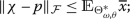
-
2:
In \(\mathscr{UHR}\) sense, concerning
 , if there is a real number
  such that for each \(\overline{x}>0\) and for each solution υ of inequality (9) there ∃ a solution υ̂ of q-
 (1) with
 such that there is a solution b of the q-
 (
(
 , if there is a real number
  such that for each
  (
(
Remark 2.1
A function \(\upsilon \in \mathcal{F}\) is considered a solution of inequality (8) iff ∃ another function  (which relies on υ) s.t. \(|\varrho (\chi )|\leqslant \overline{x}\) for every \(\chi \in \Lambda \) and
3 Existence and uniqueness results
In this section, we investigate the 1\(\mathfrak{EU}\) of solution of problem (1).
Lemma 3.1
Consider \(\phi \in \mathcal{C}(\Lambda )\). Thus, the solution of problem

for \(0<\max \{ \alpha ,\omega , \theta \} \leqslant 1\),  is given as

where \(\phi \in \mathcal{F}\) is given as
and  .
.
Proof
Now, let us consider
Applying the operator \(\mathcal{I}_{q}^{\alpha}\) on both sides of (12) and employing Lemma 2.6 with \(n=1\), we obtain

Now, using the operator \(\mathcal{I}_{q}^{\omega}\), (1) of Lemma 2.5, (a) of Lemma 2.7, and applying the same procedure on both sides of (13), we get

It follows that
where  , (\(j=0,1,2\)). Using boundary constraints

Now, using the L.H.S of (16) in (15), we obtain
Similarly, using the R.H.S of (16) in (15), we obtain

Thus (16) becomes

By the 2nd boundary condition,
Applying \({}^{\mathscr{C} }\mathbb{D}^{\theta}_{q}\), (3) of Lemma 2.5 and (b) of Lemma 2.7 on both sides of (15), we get
Now, applying \({}^{\mathscr{C} }\mathbb{D}^{\omega}_{q}\) and the same procedure on both sides of (18), we get
So, Eq. (19) becomes \({}^{\mathscr{C} }\mathbb{D}^{\omega}_{q} ({}^{\mathscr{C} } \mathbb{D}^{\theta}_{q} \upsilon (\chi ))|_{\chi =\delta}= \mathcal{I}_{q}^{\alpha}\phi (\delta )+c_{0}\). By Eq. (17), we get \(c_{0} = - \mathcal{I}_{q}^{\alpha} \phi (\delta )\). Using the 3rd boundary condition,

Now, using the L.H.S of (20) in (15), we get
So, at \({}^{\mathscr{C} }\mathbb{D}_{q}^{ \beta} \upsilon ( \chi )|_{ \chi =0}=c_{1}\), since \(\theta -\beta \leqslant 0\) by Eq. (2). Now, using the R.H.S of (20) in (15), we have

So, (20) becomes

Putting all values in (15), we obtain

and

□
We define an operator \(\rho :\mathcal{F}\rightarrow \mathcal{F}\) by applying Lemma 3.1 as follows:

The following assumptions will be used in our upcoming results:
- \(\mathrm{(H_{1})}\):
-
 ;
; - \(\mathrm{(H_{2})}\):
-
 are continuous;
 - \(\mathrm{(H_{3})}\):
-
∃ constant \(\overline{y}>0\) in such a way that ∀ \(\chi \in {\Lambda}\) and
 , \(m=\{1,2,3\}\), we get $$ \bigl\vert {\xi}(\chi , \upsilon _{1}, \upsilon _{2}, \upsilon _{3} )-{\xi}( \chi ,\hat{ \upsilon}_{1}, \hat{ \upsilon}_{2},\hat{ \upsilon}_{3}) \bigr\vert \leqslant \sum _{m=1}^{3}\overline{y}_{m} \vert \upsilon _{m}- \hat{ \upsilon}_{m} \vert ; $$
 - \(\mathrm{(H_{4})}\):
-
∃ constant \(\overline{z}>0\) in such a way that ∀ \(\chi \in {\Lambda}\) and
 , \(v=\{1,2,3\}\), we have $$ \bigl\vert {g}(\upsilon , \upsilon _{1}, \upsilon _{2}, \upsilon _{3})-{g}( \chi ,\hat{\upsilon}_{1}, \hat{ \upsilon}_{2},\hat{\upsilon}_{3}) \bigr\vert \leqslant \sum _{v=1}^{3}\overline{z}_{v} \vert \upsilon _{v}- \hat{\upsilon}_{v} \vert ; $$
 - \(\mathrm{(H_{5})}\):
-
∃ real constants \(\varphi _{m}\geq 0\) (\(m=1,2,3\)) and \(\varphi _{0}>0\) in such a way that for any
 (\(m=1,2,3\)) we have $$ \bigl\vert {\xi}(\chi , \upsilon _{1}, \upsilon _{2}, \upsilon _{3}) \bigr\vert \leqslant \varphi _{0}+\varphi _{1} \vert \upsilon _{1} \vert +\varphi _{2} \vert \upsilon _{2} \vert + \varphi _{3} \vert \upsilon _{3} \vert ; $$
 - \(\mathrm{(H_{6})}\):
-
∃ real constants \(\wp _{v}\geq 0\) \((v=1,2,3)\) and \(\wp _{0}>0\) in such a way that for any
 (\(v=1,2,3\)) we have $$ \bigl\vert {g}(\chi , \upsilon _{1}, \upsilon _{2}, \upsilon _{3}) \bigr\vert \leqslant \wp _{0}+\wp _{1} \vert \upsilon _{1} \vert +\wp _{2} \vert \upsilon _{2} \vert +\wp _{3} \vert \upsilon _{3} \vert ; $$
 - \(\mathrm{(H_{7})}\):
-
∃ an increasing
 and \(\vartheta _{h}>0\), then the following inequality $$ \mathcal{I}_{q }^{ \alpha + \omega +\theta} h(\chi ) \leqslant \vartheta _{h} {h(\chi )},\quad \chi \in \Lambda , $$
is satisfied.
 ;
; are continuous;
 ,
,  ,
,  (
( (
( and
and In the following sections, we will employ the fixed point theory to confirm \(\mathfrak{EU}\) of solution of q-fractional \(\mathcal{J}\) problem outlined in (1). For simplicity, the following notations will be used in our upcoming results:

Theorem 3.2
Suppose that assumptions \(\mathrm{(H_{2})}\), \(\mathrm{(H_{3}),}\) and \(\mathrm{(H_{4})}\) hold. Thus, q- (1) has a unique solution if
where \(\varpi _{i}\), \(i=1,2,3\), are given by (21).
Proof
First, we demonstrate that \(\rho{\mathcal{W}}_{\epsilon}\subset \mathcal{W}_{\epsilon} \), where \(\mathcal{W}_{\epsilon}= \{ \upsilon \in \mathcal{F}:\|\upsilon \|_{\mathcal{F}}\leqslant \epsilon \}\) with
s.t. \(\Pi = \sup_{ \chi \in \Lambda} | \xi (\chi ,0,0,0)|\), \(\psi = \sup_{\chi \in \Lambda}| g( \chi ,0,0,0)|\), and \(\varpi _{i}\), \(i=1,2,3\), are given by (21). Using \(\mathrm{(H_{3})}\) and \(\mathrm{(H_{4})}\), we get
Then we get

Now, using (23), we obtain

Also, we have

and

From the definition of \(\|\cdot \|_{ \mathcal{F}}\), we have
which means that \(\rho \mathcal{W}_{\epsilon}\subset \mathcal{W}_{\epsilon}\). We now demonstrate that the ρ is an operator for a contraction mapping. Now \(\upsilon , \hat{\upsilon}\in \mathcal{W}_{\epsilon}\) and \(\chi \in \Lambda \), we obtain

By \(\mathrm{(H_{3})}\) and \(\mathrm{(H_{4})}\), we obtain

Also, by using \(\mathrm{(H_{3})}\) and \(\mathrm{(H_{4})}\), we obtain

and

Thus, we get
We observe that ρ is a contraction operator by using (22). We infer that ρ has a unique fixed point that is a solution of (1) as a result of Lemma 2.9. □
By applying Lemma 2.8, we explore certain conditions where q- (1) has at least one solution in Theorem 3.2.
Theorem 3.3
Assume that hypotheses \(\mathrm{(H_{5})}\) and \(\mathrm{(H_{6})}\) hold. If
is satisfied, then the proposed problem described by (1) has at least one solution within the domain Λ.
Proof
Our initial goal is to investigate the complete continuity of an operator \(\rho : \mathcal{F} \rightarrow \mathcal{F}\). Considering function’s continuity Θ, we can also conclude that the operator ρ is also continuous. Assume that \(\kappa \subset \mathcal{F}\) is bounded. Then there exists a positive constant \(\mathfrak{P}\) s.t. \(| \Theta ^{*}_{\upsilon , \omega ,\theta}(s)|\leqslant \mathfrak{P}\) for each \(\upsilon \in \kappa \). Then, for any \(\upsilon \in \kappa \) and using (21), we can find that
The inequalities indicate that an operator ρ remains uniformly bounded. Furthermore, we will verify that ρ is equicontinuous. For \(\upsilon \in \Lambda \) and  , we get

Also, we obtain
and
The right-hand sides of (25), (26), (27) tend to zero independently of υ as \(\chi _{1}\rightarrow \chi _{2}\). Therefore, an operator \(\rho : \mathcal{F} \to \mathcal{F}\) is completely continuous by Arzelà–Ascoli theorem. Finally, we show that a set \(\Upsilon = \{ \upsilon \in \mathcal{F} : \upsilon = \varepsilon \rho (\upsilon ), 0 < \varepsilon <1 \}\) is bounded. Let \(\upsilon \in \Upsilon \), thus \(\upsilon = \varepsilon \rho ( \upsilon )\). For every \(\chi \in \Lambda \), we have \(\upsilon (\chi )=\varepsilon \rho \upsilon (\chi )\). Then
We also have
which implies that
Consequently,
where \(\varpi _{i}, i=1,2,3\), are given by (21). From (28), we see that \(\|\upsilon \|_{\mathcal{F}}\leqslant \infty \). As a result, ϒ is bounded. We deduce that an operator ρ has a fixed point, which is the solution of q- (1) as a result of Lemma 2.8. □
4 Stability results
We study the \(\mathscr{UH}\) and \(\mathscr{UHR}\) stability [46] of q- in this section.
Theorem 4.1
Assume that \(\mathrm{(H_{2})}\)–\(\mathrm{(H_{4})}\) and (22) hold. Then the q- (1) is \(\mathscr{UH}\) stable.
Proof
Consider \(\hat{\upsilon}\in \mathcal{F}\) to be the only solution to the problem

for \(\chi \in{ \Lambda}\), WHERE \(0 < \alpha , \omega ,\theta \leqslant \Lambda \). So that inequality (8) can be solved with υ in \(\mathcal{F}\). Utilizing Remark 2.1, we obtain
where  , \(j=\{0,1,2\}\), \(\phi _{\upsilon} ( \chi ) = \Theta ^{*}_{\upsilon ,\omega ,\theta}( \chi )\), and \(|\varrho (\chi )|\leqslant \overline{x}\), \(\chi \in \Lambda \). Thanks to Lemma 3.1,

Also, we have
\(\mathrm{(H_{3})}\) and \(\mathrm{(H_{4})}\) imply that

where Eq. (21) provides \(\varpi _{i}\), \(i=\{1,2,3\}\). Next

If we put

we obtain  . As a result, the q-
 (1) is \(\mathscr{UH}\) stable. □
Theorem 4.2
Suppose that \(\mathrm{(H_{2})}\)–\(\mathrm{(H_{4})}\), \(\mathrm{(H_{7}),}\) and (22) hold. Then q- (1) is \(\mathscr{UHR}\) stable in relation to h.
Proof
We have
where \(\chi \in \Lambda \),  , \(j=0,1,2\), and \(|\varrho (\chi )|\leqslant \overline{x} h(\chi )\), and inequality (9) can be solved by using \(\upsilon \in \mathcal{F}\). Taking \(\hat{\upsilon}\in \mathcal{F}\) as the singular solution of (29), by Lemma 3.1, we have
Also, we have
So, by \(\mathrm{(H_{3})}\), \(\mathrm{(H_{4})}\), and \(\mathrm{(H_{7})}\), we obtain
Then we get
If we take

we can obtain  considering \(\chi \in \Lambda \). Consequently, the \(\mathscr{UHR}\) stability is achieved by q-
 (1). □
5 Examples and illustrative results
In this section, we check the correctness of the results by showing several examples. In the first example, we test q-Caputo fractional  with \(\mathbb{ABC}\)s (1) for the changes of q in the range of zero and one according to the proposed theorems.
Example 5.1
Let
where \(q\in \{ \frac {1}{5},\frac {2}{5}, \frac {3}{5} \} \subseteq (0,1)\), \(\alpha = \frac {1}{3} \in (0,1] \), \(\omega =\frac {4}{5} \in (0,1]\), \(\nu = \zeta = \frac {3}{2}\), \(\theta = \frac {3}{4}\in (0,1]\),  , \(\beta = \frac {5}{9} \in (0,1]\),
  , and
, and
where \(\overline{x}>0\),  , and
, and
For \(\chi \in \Lambda \) and  , \(m=1,2,3\), we obtain
and similarly for  , \(v=1,2,3\), we get
Therefore, conditions \(\mathrm{(H_{3})}\) and \(\mathrm{(H_{4})}\) are satisfied with
Furthermore, thanks to Eq. (21), we get

and

The data in Table 1 show the values of \(\varpi _{i}\), \(i=1,2,3\), for three different values q. Because the relations of q-calculators depend on the number of repetitions n, after several steps, their value is fixed. This mathematical performance can be clearly seen in Tables 1 and 2. The approach is similar to each group of curves in Figs. 1a, 1b, and 1c, aligning with each other and reaching a stable value that precisely determines the correctness of the argument. By (22), we get
The numerical values of relation (33) are shown in Table 2. It can be seen that after stabilizing the data of each column, these results are less than one (see Fig. 2). Therefore, the given q- (30) is addressed in Theorem 3.2, asserting that it possesses a unique solution within the interval Λ. Additionally, Theorem 4.1 states that the same q-
 (30) is \(\mathscr{UH}\) stable having

In general, as q approaches 1, we will achieve stability of the results with a higher number of iterations. For \(h ( \chi ) = \chi ^{\frac{\ln (3)}{5}}\), we obtain
Table 3 shows these results. In addition, the curves drawn in Figs. 3a and 3b confirm the existence of \(\vartheta _{h}\) and Ineq. (34) variables. Therefore, condition \(\mathrm{(H_{7})}\) is fulfilled with \(h(\chi ) = \chi ^{\frac{\ln (3)}{5}}\) and \(\vartheta _{h}=0.0834, 0.1173, 0.1066\) whenever \(q= \frac {1}{5}, \frac {2}{5}, \frac {3}{5}\), respectively. Theorem 4.2 indicates that the q- is \(\mathscr{UHR}\) (30) stable s.t.

 (
(
 (
(
 (
(The next example shows the proven facts for changes in the order of the derivative α.
Example 5.2
We consider the q-Caputo fractional  with \(\mathbb{ABC}\)s (30) in Example 5.1
with the difference that \(q=\frac {3}{5}\) is fixed and α chooses \(\{ \frac {1}{8},\frac {1}{6}, \frac {1}{3} \} \subseteq (0,1)\), \(\omega =\frac {4}{5} \), \(\nu = \zeta = \frac {8}{5}\), \(\theta = \frac {3}{4}\), \(\delta = \frac {7}{11}\), \(\beta = \frac {5}{9} \),  , and
, and
where \(\overline{x}>0\),  , and \(\Theta ^{*}_{\upsilon , \frac{4}{5}, \frac{3}{4}}(\chi )\) is defined by (31). It was found that conditions \(\mathrm{(H_{3})}\) and \(\mathrm{(H_{4})}\) are satisfied with \(\overline{y}_{1} = \frac {\sqrt{15}}{123}\), \(\overline{y}_{2} = \frac {1}{333{\sqrt{ \ln 12}}}\), \(\overline{y}_{3} = \frac {1}{66}\), and \(\overline{z}_{1} = \frac { \sqrt{e^{2}}}{435}\), \(\overline{z}_{2} = \frac {1}{345{ \sqrt{e^{19}}}}\), \(\overline{z}_{3} = \frac {1}{137 \ln ( \sqrt{35}) }\). Thanks to Eq. (21), by using these data, we obtain
  and
and

The data in Table 4 show the values of \(\varpi _{i}\), \(i=1,2,3\), for three different values of derivative order α. The approach is similar to each group of curves in Figs. 4a, 4b, and 4c, aligning with each other and reaching a stable value that precisely determines the correctness of the argument. By (22), we get
The numerical values of relation (36) are shown in Table 5. It can be seen that after stabilizing the data of each column, these results are less than one (see Fig. 5). Therefore, the given q- (35) is addressed in Theorem 3.2, asserting that it possesses a unique solution within the interval Λ. Additionally, Theorem 4.1 states that the same q-
 (35) is \(\mathscr{UH}\) stable having

For \(h ( \chi ) = \chi ^{\frac{\ln (3)}{5}}\), we have
Table 5 shows these results. In addition, the curves drawn in Figs. 6a and 6b confirm the existence of \(\vartheta _{h}\) and Ineq. (37) variables. Therefore, condition \(\mathrm{(H_{7})}\) is fulfilled with \(h(\chi ) = \chi ^{\frac{\ln (3)}{5}}\) and \(\vartheta _{h}=0.097, 0.099, 0.107\) whenever \(\alpha = \frac {1}{5}, \frac {2}{5}, \frac {3}{5}\), respectively. Theorem 4.2 indicates that the q- is \(\mathscr{UHR}\) (35) stable s.t.

 (
(
 (
(
 (
(
MATLAB lines for calculation q-factorial function

MATLAB lines for q-gamma function

MATLAB lines to calculate q-integral
6 Conclusion
We analyzed the q- , involving both \(\mathbb{ABC}s\) and q-fractional \(\mathscr{CD}s\). Our main focus was on establishing certain conditions that guaranteed the \(\mathfrak{EU}\) of solution. For the validity of the suggested system, given in (1), we employed the Banach fixed point theorem and Leray-Schauder alternative. Additionally, we also explored the \(\mathscr{US}\) outcomes and examined the resolution of our model (1) in specific circumstances. Our primary theoretical findings are demonstrated by means of a few examples.
Data Availability
No datasets were generated or analysed during the current study.
References
Jackson, F.H.: On q-functions and certain difference operator. Trans. R. Soc. Edinb. 46(2), 253–281 (1909). https://doi.org/10.1017/S0080456800002751
Hajiseyedazizi, S.N., Samei, M.E., Alzabut, J., Chu, Y.: On multi-step methods for singular fractional q-integro-differential equations. Open Math. 9, 1378–1405 (2021). https://doi.org/10.1515/math-2021-0093
Houas, M., Samei, M.E.: Existence and stability of solutions for linear and nonlinear damping of q-fractional Duffing-Rayleigh problem. Math. Methods Appl. Sci. 20(7), 148 (2023). https://doi.org/10.1007/s00009-023-02355-9
Lachouri, A., Samei, M.E., Ardjouni, A.: Existence and stability analysis for a class of fractional pantograph q-difference equations with nonlocal boundary conditions. Bound. Value Probl. 2023, 2 (2023). https://doi.org/10.1186/s13661-022-01691-1
Samei, M.E., Fathipour, A.: Existence and stability results for a class of nonlinear fractional q-integro-differential equation. Int. J. Nonlinear Anal. Appl. 14(7), 143–158 (2023). https://doi.org/10.22075/ijnaa.2022.7128
Houas, M., González, F.M., Samei, M.E., Kaabar, M.K.A.: Uniqueness and Ulam-Hyers-Rassias stability results for sequential fractional pantograph q-differential equations. J. Inequal. Appl. 2022, 93 (2022). https://doi.org/10.1186/s13660-022-02828-7
Shabibi, M., Samei, M.E., Ghaderi, M., Rezapour, S.: Some analytical and numerical results for a fractional q-differential inclusion problem with double integral boundary conditions. Adv. Differ. Equ. 2021, 466 (2021). https://doi.org/10.1186/s13662-021-03623-2
Houas, M., Samei, M.E.: Existence and stability of solutions for linear and nonlinear damping of q-fractional Duffing-Rayleigh problem. Mediterr. J. Math. 20, 148 (2023). https://doi.org/10.1007/s00009-023-02355-9
Samei, M.E., Ahmadi, A., Selvam, A.G.M., Alzabut, J., Rezapour, S.: Well-posed conditions on a class of fractional q-differential equations by using the Schauder fixed point theorem. Adv. Differ. Equ. 2021, 482 (2021). https://doi.org/10.1186/s13662-021-03631-2
Abdi, W.H.: On q-Laplace transforms. Proc. Natl. Acad. Sci. India Sect. A Phys. Sci. 29(4), 89–408 (1960)
Agarwal, R.P.: Certain fractional q-integrals and q-derivatives. Math. Proc. Camb. Philos. Soc. 66, 365–370 (1969). https://doi.org/10.1017/S0305004100045060
Kac, V., Cheung, P.: Quantum Calculus. Springer, NewYork (2002)
Lachouri, A., Samei, M.E., Ardjouni, A.: Existence and stability analysis for a class of fractional pantograph q-difference equations with nonlocal boundary conditions. Bound. Value Probl. 2023, 2 (2023). https://doi.org/10.1186/s13661-022-01691-1
Ferreira, R.A.C.: Nontrivial solution for fractional q-difference boundary value problem. Electron. J. Qual. Theory Differ. Equ. 2010, 70 (2010). https://doi.org/10.14232/ejqtde.2010.1.70
Samei, M.E., Karimi, L., Kaabar, M.K.A.: To investigate a class of multi-singular pointwise defined fractional q-integro-differential equation with applications. AIMS Math. 7(5), 7781–7816 (2022). https://doi.org/10.3934/math.2022437
Gaulue, L.: Some results involving generalized Eedèlyi-Kober fractional q-integral operators. Rev. Tecnol. Cient. URU 6, 77–89 (2014)
Gottleib, H.P.W.: Simple nonlinear jerk functions with periodic solutions. Am. J. Phys. 66(10), 903–906 (1998). https://doi.org/10.1119/1.18980
Schot, S.H.: Jerk: the time rate of change of acceleration. Am. J. Phys. 46(11), 1090–1094 (1978). https://doi.org/10.1119/1.11504
Rothbart, H.A., Wahl, A.M.: Mechanical designs and systems handbook. J. Appl. Mech. 32, 478 (1965)
El-Nabulsi, R.A.: Jerk in planetary systems and rotational dynamics, nonlocal motion relative to Earth and nonlocal fluid dynamics in rotating Earth frame. Earth Moon Planets 122(3), 15–41 (2018). https://doi.org/10.1007/s11038-018-9519-z
Samei, M.E., Yang, W.: Existence of solutions for k-dimensional system of multi-term fractional q-integro-differential equations under anti-periodic boundary conditions via quantum calculus. Math. Methods Appl. Sci. 43(7), 4360–4382 (2020). https://doi.org/10.1002/mma.6198
Linz, S.J.: Nonlinear dynamical models and jerk motion. Am. J. Phys. 65(1), 523–526 (1997). https://doi.org/10.1119/1.18594
Wang, X., Berhail, A., Tabouche, N., Matar, M.M., Samei, M.E., Kaabar, M.K.A., Yue, X.G.: A novel investigation of non-periodic snap \(bvp\) in the \(\mathbb{G}\)-Caputo sense. Axioms 11, 390 (2022). https://doi.org/10.3390/axioms11080390
Abdeljawad, T., Samei, M.E.: Applying quantum calculus for the existence of solution of q-integro-differential equations with three criteria. Discrete Contin. Dyn. Syst., Ser. S 14(10), 3351–3386 (2021). https://doi.org/10.3934/dcdss.2020440
Rahman, M.S., Hassan, A.S.M.Z.: Modified harmonic balance method for the solution of nonlinear jerk equations. Results Phys. 8, 893–897 (2018). https://doi.org/10.1016/j.rinp.2018.01.030
Messias, M., Silva, R.P.: Determination of nonchaotic behavior for some classes of polynomial jerk equations. Int. J. Bifurc. Chaos 30, 1–12 (2020)
Ismail, G., Abu-zinadah, H.H.: Analytic approximations to non-linear third order jerk equations via modified global error minimization method. J. King Saud Univ., Sci. 33(1), 101219 (2021). https://doi.org/10.1016/j.jksus.2020.10.016
Rajković, P.M., Marinković, S.D., Stanković, M.S.: On q-analogue of Caputo derivatives and Mittag-Leffler function. Fract. Calc. Appl. Anal. 10, 359–373 (2007)
Sousa, J.V.d.C., Kucche, K.D., de Oliveira, E.C.: Stability of ψ-Hilfer impulsive fractional differential equations. Appl. Math. Lett. 88, 73–80 (2019). https://doi.org/10.1016/j.aml.2018.08.013
Wang, J.R., Zada, A., Waheed, H.: Stability analysis of a coupled system of nonlinear implicit fractional anti-periodic boundary value problem. Math. Methods Appl. Sci. 42(18), 6706–6732 (2019). https://doi.org/10.1002/mma.5773
Sousa, J.V.d.C., de Oliveira, E.C.: On the ψ-Hilfer fractional derivative. Commun. Nonlinear Sci. Numer. Simul. 60, 72–91 (2018). https://doi.org/10.1016/j.cnsns.2018.01.005
Sousa, J.V.d.C., Frederico, G.S.F., de Oliveira, E.C.: ψ-Hilfer pseudo-fractional operator: new results about fractional calculus. Comput. Appl. Math. 39, 254 (2020). https://doi.org/10.1007/s40314-020-01304-6
Thabet, S.T.M., Vivas-Cortez, M., Kedim, I., Samei, M.E., Ayari, M.I.: Solvability of ϱ-Hilfer fractional snap dynamic system on unbounded domains. Fractal Fract. 7(8), 607 (2023). https://doi.org/10.3390/fractalfract7080607
Sousa, J.V.d.C., Jarad, F., Abdeljawad, T.: Existence of mild solutions to Hilfer fractional evolution equations in Banach space. Ann. Funct. Anal. 12, 12 (2021). https://doi.org/10.1007/s43034-020-00095-5
Haddouchi, F., Samei, M.E., Rezapour, S.: Study of a sequential ψ-Hilfer fractional integro-differential equations with nonlocal BCs. J. Pseudo-Differ. Oper. Appl. 14, 61 (2023). https://doi.org/10.1007/s11868-023-00555-1
Sousa, J.V.d.C., de Oliveira, E.C.: Fractional order pseudoparabolic partial differential equation: Ulam-Hyers stability. Bull. Braz. Math. Soc. 50, 481–496 (2019). https://doi.org/10.1007/s00574-018-0112-x
Haddouchi, F., Samei, M.E.: Solvability of a φ-Riemann-Liouville fractional boundary value problem with nonlocal boundary conditions. Math. Comput. Simul. 219, 355–377 (2024). https://doi.org/10.1016/j.matcom.2023.12.029
Houas, M., Samei, M.E., Rezapour, S.: Solvability and stability for a fractional quantum jerk type problem including Riemann-Liouville-Caputo fractional q-derivatives. Partial Differ. Equ. Appl. Math. 7, 100514 (2023). https://doi.org/10.1016/j.padiff.2023.100514
Jackson, F.H.: q-Difference equations. Am. J. Math. 32(10), 305–314 (1910). https://doi.org/10.2307/2370183
Bohner, M., Peterson, A.: Dynamic Equations on Time Scales. Birkhäuser, Boston (2001)
Samei, M.E., Zanganeh, H., Aydogan, S.M.: Investigation of a class of the singular fractional integro-differential quantum equations with multi-step methods. J. Math. Ext. 15, 1–54 (2021). https://doi.org/10.30495/JME.SI.2021.2070
Adam, C.R.: The general theory of a class of linear partial q-difference equations. Trans. Am. Math. Soc. 26(3), 283–312 (1924)
Annaby, M., Mansour, Z.: q-Fractional Calculus and Equations. Springer, Heildberg (2012). https://doi.org/10.1007/978-3-642-30898-7
Granas, A., Dugundji, J.: Fixed Point Theory. Springer, New York (2003)
Smart, D.R.: Fixed Point Theorems. Cambridge University Press, Cambridge (1980)
Rus, I.A.: Ulam stabilities of ordinary differential equations in Banach space. Carpath. J. Math. 26(1), 103–107 (2010)
Acknowledgements
Not applicable.
Funding
Not applicable.
Author information
Authors and Affiliations
Contributions
KHK: Actualization, methodology, formal analysis, validation, investigation and initial draft. AZ: Formal analysis, methodology, validation, investigation and initial draft. ILP: Methodology, formal analysis, validation and investigation. MES: Methodology, formal analysis, validation, actualization, investigation, software, simulation, initial draft and was a major contributor in writing the manuscript. All authors read and approved the final manuscript.
Corresponding author
Ethics declarations
Ethics approval and consent to participate
Not applicable.
Consent for publication
Not applicable.
Competing interests
The authors declare no competing interests.
Additional information
Publisher’s Note
Springer Nature remains neutral with regard to jurisdictional claims in published maps and institutional affiliations.
Supplement
Supplement
Rights and permissions
Open Access This article is licensed under a Creative Commons Attribution 4.0 International License, which permits use, sharing, adaptation, distribution and reproduction in any medium or format, as long as you give appropriate credit to the original author(s) and the source, provide a link to the Creative Commons licence, and indicate if changes were made. The images or other third party material in this article are included in the article’s Creative Commons licence, unless indicated otherwise in a credit line to the material. If material is not included in the article’s Creative Commons licence and your intended use is not permitted by statutory regulation or exceeds the permitted use, you will need to obtain permission directly from the copyright holder. To view a copy of this licence, visit http://creativecommons.org/licenses/by/4.0/.
About this article

Cite this article
Khalid, K.H., Zada, A., Popa, IL. et al. Existence and stability of a q-Caputo fractional jerk differential equation having anti-periodic boundary conditions. Bound Value Probl 2024, 28 (2024). https://doi.org/10.1186/s13661-024-01834-6
Received:
Accepted:
Published:
DOI: https://doi.org/10.1186/s13661-024-01834-6