Group Actions on Twisted Sums of Banach Spaces

Abstract

We study bounded actions of groups and semigroups G on exact sequences of Banach spaces from the point of view of (generalized) quasilinear maps, characterize the actions on the twisted sum space by commutator estimates and introduce the associated notions of G-centralizer and G-equivariant map. We will show that when (A) G is an amenable group and (U) the target space is complemented in its bidual by a G-equivariant projection, then uniformly bounded compatible families of operators generate bounded actions on the twisted sum space; that compatible quasilinear maps are linear perturbations of G-centralizers; and that, under (A) and (U), G-centralizers are bounded perturbations of G-equivariant maps. The previous results are optimal. Several examples and counterexamples are presented involving the action of the isometry group of $L_p(0,1), p\ne 2$ on the Kalton–Peck space $Z_p$, certain non-unitarizable triangular representations of the free group ${\mathbb {F}}_\infty$ on the Hilbert space, the compatibility of complex structures on twisted sums, or bounded actions on the interpolation scale of $L_p$-spaces. In the penultimate section we consider the category of G-Banach spaces and study its exact sequences, showing that, under (A) and (U), G-splitting and usual splitting coincide. The purpose of the final section is to present some applications, showing that several previous result are optimal and to suggest further open lines of research.

1 Introduction

This paper emerges from the observation of similarities between different problems:

• (a) The construction of non-unitarizable, bounded, representations of the free group ${\mathbb {F}}_\infty$ on the Hilbert space.

• (b) The construction of operators on the Kalton–Peck space $Z_2$.

• (c) The differential process associated to a complex interpolation scheme.

• (d) Actions of groups on exact sequences of Banach spaces.

• (e) The existence of certain bounded groups of isomorphisms on the space $c_0$.

In all cases, certain non-linear maps (including sometimes linear unbounded maps) and their compatibility with the action of some groups of operators through commutator estimates are at the core of the problem. In (a), a linear unbounded map used to define a non-inner derivation and therefore a non-unitarizable representation [43]; in (b) the Kalton–Peck map $\textsf{KP}$ [37] (see also [7, Section 3.2]); in (c) is the “$\Omega$-operator" mentioned by several authors Cwikel et al. [23, Section I], Rochberg [44], Carro [14]... And in (d) we encounter the Banach version of the three-representation problem (see [38]). Another unexpected example (e) is a linear unbounded map used in [1] to define a non-trivial derivation in a study of bounded groups acting on $c_0$. Connections between some of those elements had been observed before: for instance, Kalton observed [34, 35] that while working on Köthe spaces, $\Omega$-operators are a special type of quasilinear map, that he called $L_\infty$-centralizers, intimately connected with the complex interpolation scale.

To obtain a unified point of view we consider a group or semigroup G, two bounded actions u, v on two Banach spaces X, Y and introduce the notion of G-centralizer $\Omega$, as well as the more general notion of a quasi-linear map $\Omega$ compatible with an u, v: this allows us to construct an exact sequence $0\longrightarrow X \rightarrow X\oplus _\Omega Y \longrightarrow Y \longrightarrow 0$ of Banach spaces and connect possible actions of G on the twisted sum space $X\oplus _\Omega Y$ with commutator estimates involving $\Omega$ and derivations of the group.

Our results move at two levels, the theoretical and the examples/counterexamples level. On the theoretical side, we present the following list of results (to simplify notation, let (A) be the condition “G is amenable" and let (U) be the condition “X is complemented in its bidual by a G-equivariant projection"):

• (1) Triangular representations of groups on the Hilbert space H may be interpreted as diagonal representations on H seen as a twisted Hilbert space.

• (2) Under (A) and (U), a uniformly bounded family $(T_g)_{g\in G}$ of operators yielding commutative diagrams

  

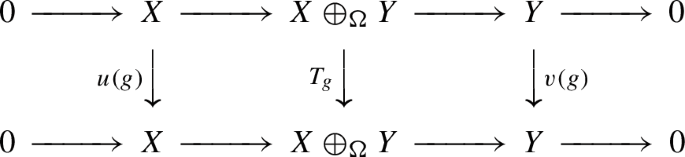
  provides a compatible action of G on $X\oplus _\Omega Y$.

• (3) Every $\Omega$ compatible with an action on $X\oplus _\Omega Y$ is a linear perturbation of a G-centralizer (possibly with values in a larger target space).

• (4) Under (A) and (U), every G-centralizer is a bounded perturbation of a G-equivariant map.

• (5) We introduce the category of G-Banach spaces and show that, under (A) and (U), a G-exact sequence of G-spaces G-splits if and only if it splits as an exact sequence of Banach spaces.

We also present the following counterexamples:

• We will use a construction of Pytlic and Szwarc [43] to show a centralizer (on $\ell _2$) that is not a bounded perturbation of an equivariant centralizer when G is non-amenable. We will provide another counterexample, inspired from [1] and defined on $c_0$, when X is not complemented in its bidual. These examples show that (4) above is optimal.

• We will show that the Kalton–Peck map is not a centralizer for the groups of isometries on $L_p, p \ne 2$ or isometries preserving disjointness on $L_2$. It is however compatible with the actions of those groups.

• In the case of the group of isometries of $L_2$, the Kalton–Peck map is not even compatible with the action of that group.

There are specific sections devoted to actions of groups on complex interpolation scales, on Kalton–Peck spaces and on higher order Rochberg spaces, as well as to the connections between G-centralizers and (almost) transitivity.

2 The Background

Let X, Y be Banach spaces. In what follows $\Delta \subset Y$ represents a dense subspace of Y (sometimes called the intersection space), while $\Sigma$ represents the ambient space. To work with quasilinear maps it would be enough that $\Sigma$ is a vector space containing X. To work in an interpolation context it is convenient asking $\Sigma$ to carry a vectorial topology making the containment map continuous; and to work with continuous actions it is better to ask that the continuous action can be extended to $\Sigma$. When necessary, we will specify the injective linear map $\jmath : X\rightarrow \Sigma$ and endow the subspace $\jmath [X]$ with the norm $\Vert \jmath (x)\Vert =\Vert x\Vert _X$. Most often than not there is a natural choice of $\Sigma$ that is already a Banach space and making $\jmath$ continuous. The section entitled “The issue of the ambient space" shows how to make, once these basic premises have been established, irrelevant the choice of the ambient space even in the most restrictive Banach setting. A homogeneous map $\Omega : \Delta \longrightarrow \Sigma$ is a z-linear map $\Delta \curvearrowright X$ if there is a constant C such that for all finite sequences of elements $y_1, \dots , y_N \in \Delta$

• (a) $\Omega (\sum _{n=1}^N y_n)- \sum _{n=1}^N \Omega (y_n)\in \jmath [X]$

• (b) $\Vert \Omega (\sum _{n=1}^N y_n)- \sum _{n=1}^N \Omega (y_n)\Vert _{\jmath [X]}\le C\sum _{n=1}^N \Vert y_n\Vert _Y$.

In this paper we mainly use the notation $\Omega : \Delta \curvearrowright X$, although $\Omega : Y \curvearrowright X$ can also be appear when the choice of $\Delta$ is clear from the context or irrelevant. When condition (b) holds only for pairs of points then $\Omega$ is called quasilinear. A quasilinear map $\Omega : \Delta \curvearrowright X$ with ambient space $\Sigma$ is said to be trivial if there is a linear (not necessarily continuous) map $L: \Delta \longrightarrow \Sigma$ such that $\Omega -L: \Delta \rightarrow \jmath [X]$ is bounded, in the sense that $\Vert \Omega (y)-L(y)\Vert _{\jmath [X]}\le M\Vert y\Vert _Y$ for some constant M and all $y\in \Delta$. Two quasilinear maps $\Phi , \Psi : \Delta \curvearrowright X$ with ambient space $\Sigma$ are said to be equivalent, and denoted $\Phi \sim \Psi$, (resp. boundedly equivalent and denoted $\Phi \sim _\flat \Psi$) if $\Phi - \Psi$ is trivial (resp. $\Phi - \Psi :\Delta \longrightarrow X$ is bounded). The twisted sum generated by a quasilinear map $\Omega$ is the completion $X \oplus _\Omega Y$ of the space $X \oplus _\Omega \Delta := \{(\omega , y) \in \Sigma \times \Delta : \omega - \Omega y \in \jmath [X]\}$ endowed with the quasi-norm $\Vert y\Vert _{Y}+\Vert \omega - \Omega y\Vert _{\jmath [X]}$. From now on, except when in need, we shall omit the embedding $\jmath$. If $\Omega$ is z-linear then $\Vert \cdot \Vert _\Omega$ is equivalent to a norm, and thus $X\oplus _\Omega Y$ is a Banach space. Kalton showed [31, Theorem 4.10] that quasilinear maps on B-convex Banach spaces (e.g. uniformly convex spaces) are z-linear; therefore, twisted sums in which the quotient space is B-convex are Banach spaces. The map $\imath :X\longrightarrow X\oplus _\Omega Y$ given by $\imath (x)=(x,0)$ is an into isomorphism and the map $\pi :X\oplus _\Omega Y\longrightarrow Y$ given by $\pi (\omega ,y)=y$ (for $y \in \Delta$, then extended by continuity) is onto. These spaces and operators form a short exact sequence that shall be referred to as the sequence generated by $\Omega$. Two exact sequences of Banach spaces are called equivalent when there is an operator T making the diagram

commute. When $Z=X\oplus _\Omega Y$ and $Z'=X\oplus _\Phi Y$ that happens if and only if $\Phi$ and $\Psi$ are equivalent maps.

Given two maps S, T, its commutator is defined as $[S,T]= ST - TS$ provided this makes sense. We will need to use a generalized commutator for three maps defined as $[u,\Omega , v] = u\Omega -\Omega v$, whenever this makes sense.

3 G-Centralizers

Definition 3.1

Let G be a semigroup. A G-space is a normed space X equipped with a bounded action $G\times X \rightarrow X$; namely, a morphism of semigroups $u: G\rightarrow {\mathfrak {L}}(X)$ such that $\gamma (u):= \sup \{\Vert u(g)\Vert : g\in G\}<\infty$.

Note that we do not require G to carry any topology and therefore there is no continuity involved with respect to G (alternatively we may think of G as discrete). Occasionally we will consider unbounded or even nonlinear actions, but that will be explicitly said. Paramount examples of bounded actions are (see the appropriate section in the paper for unexplained terms): (a) The action of the group of units ${\mathcal {U}}$ of $L_\infty (S, \mu )$ on either $L_\infty$-Banach modules or Köthe spaces. In particular, the action of the Cantor group $2^\omega =\{-1,+1\}^{\mathbb {N}}$ on spaces with unconditional basis or that of the group $2^{<\omega }$ of elements of $2^\omega$ that are eventually 1 on c. (b) The action of the group generated by measure preserving rearrangements of the base space and change of signs on rearrangement invariant Köthe spaces. (c) The action of the group $\textrm{Isom}(X)$ of isometries of X on X. (d) The action of the group $\mathrm{Isom_{disj}}(L_2)$ of isometries that preserve disjointness on $L_2$. (e) The natural left regular action of the free group ${\mathbb {F}}_\infty$ on the Hilbert space seen as $\ell _2({\mathbb {F}}_\infty )$. Note that in the above, example (a) satisfies (A) but, in the case of c, not (U); examples (d) and (e) satisfy (U) and not (A); and the case for (b)(c) depends on the choice of the space.

Given an exact sequence $0\rightarrow X\rightarrow Z\rightarrow Y\rightarrow 0$ of G-spaces, we will agree for the rest of this paper that the action of G on X will be denoted u, that on Y will be denoted v and that on Z will be denoted $\lambda$.

Definition 3.2

Let G be a semigroup.

• G-operator: An operator (resp. a linear map) $T: X\rightarrow Y$ between two G-spaces X and Y is a G-operator (resp. a G-linear map) if $v(g)T=Tu(g)$ for all $g \in G$.

• G-subspace: A G-subspace $Y'$ of Y is a subspace of Y such that the canonical inclusion $\imath : Y'\rightarrow Y$ is a G-operator; in which case we shall also occasionally say that Y is a G-superspace of $Y'$.

• G-centralizer: Let Y, X be G-spaces, let $\Delta \subset Y$ be a dense G-subspace of Y, and let $\Sigma \supset X$ be a G-superspace of X. A quasilinear map $\Omega : \Delta \curvearrowright X$ with ambient space $\Sigma$ is said to be a G-centralizer if the family of maps $[u(g),\Omega ,v(g)]$ takes values in X and is uniformly bounded, i.e., there exists a constant $G(\Omega )>0$ such that $\Vert u(g)\Omega y-\Omega v(g) y\Vert _X \le G(\Omega ) \Vert y\Vert _Y$ for all $g \in G$ and $y\in \Delta$.

We shall sometimes say that $\Omega$ is a centralizer compatible with G. To avoid confusion, let us make explicit that in the above we use the same letter for an action on a G-space and for the action by restriction on a G-subspace; for example for any $g \in G$, u(g) extends to a map on $\Sigma$ still denoted u(g).

It will spare us a few headaches to briefly discuss the roles of the “ambient" and “intersection" spaces $\Sigma$ and $\Delta$. Observe that $\Omega$ is in principle only defined on $\Delta$, not in Y. It is well known [37, Theorem 3.1] that every quasilinear map $\Omega : \Delta \curvearrowright X$ can be extended to a quasilinear map ${\widehat{\Omega }}: Y\longrightarrow X$, but replacing $\Omega$ by this “artificial" ${\widehat{\Omega }}$ may spoil the compatibility conditions with G, so this approach is not recommended for us.

The Issue of the Ambient Space. We need here the construction of the pushout space ${\text {PO}}$ of two operators $a: X\longrightarrow A$ and $b: X\longrightarrow B$ (the reader is referred to [7] for full details), which is the space ${\text {PO}}= (A\oplus _1 B)/ \overline{ \{(a x, -bx): x\in X\}}$ together with the operators $p_A: A\longrightarrow {\text {PO}}$ and $p_B: B \longrightarrow {\text {PO}}$ given by $p_A(x)= [(x, 0)]$ (the class of (x, 0)) and $p_B(y)=[(0,y)]$ so that one gets a commutative diagram

When one of the operators a, b is an isomorphic embedding then ${\text {PO}}= (A\oplus _1 B)/\{(a x, -bx): x\in X\}$. Assume now that one has two quasilinear maps $\Omega , \Phi : Y\curvearrowright X$, one taking values in the ambient space $\Sigma$ with embedding $\jmath : X \rightarrow \Sigma$ and the second in the ambient space $\Xi$ with embedding $\imath : X\rightarrow \Xi$. Form the pushout commutative diagram

and thus, replacing $\Omega$ by $\sigma \Omega : Y\curvearrowright \sigma \jmath [X]$ and $\Phi$ by $\xi \Phi : Y\curvearrowright \xi \imath [X]$, and calling ${\mathcal {X}}= \sigma \jmath [X]=\xi \imath [X]$, then $\sigma \Omega$ and $\xi \Phi$ are quasilinear maps $Y\curvearrowright {\mathcal {X}}$ with ambient space ${\text {PO}}$. We can extend the equivalence notion to quasilinear maps with different ambient spaces, maintaining the notation: $\Omega \sim \Phi$ means $\sigma \Omega \sim \xi \Phi$. The modification is acceptable since $\Omega \sim \Phi$ if and only if $\sigma \Omega$ and $\xi \Phi$ generate equivalent exact sequences: if $B= \sigma \Omega - \xi \Phi - L: Y\rightarrow {\mathcal {X}}$ is bounded for some linear map $L: Y\rightarrow {\text {PO}}$ then the following sequences are equivalent

(1)

via the operator $T(\sigma \jmath x, y)= (\sigma \jmath x - Ly, y)$: indeed, $(\sigma \jmath x - Ly, y)\in {\mathcal {X}}\oplus _{\xi \Phi } Y$ because $\sigma \jmath x - Ly - \xi \Phi y = \sigma \jmath x - \sigma \Omega y + By \in {\mathcal {X}}$ since $B: Y\rightarrow {\mathcal {X}}$. Since

$$\begin{aligned} \Vert T(\sigma \jmath x, y)\Vert _{\xi \Phi }= & {} \Vert (\sigma \jmath x - Ly, y)\Vert _{\xi \Phi } \\= & {} \Vert \sigma \jmath x - Ly - \xi \Phi y) \Vert + \Vert y\Vert \\= & {} \Vert \sigma \jmath x - \sigma \Omega y + By \Vert + \Vert y\Vert \\\le & {} (\Vert B\Vert +1) (\Vert \sigma \jmath x - \sigma \Omega y\Vert + \Vert y\Vert )\\\le & {} (\Vert B\Vert +1) \Vert (\sigma \jmath x, y\Vert _{\sigma \Omega } \end{aligned}$$

T is bounded, hence an isomorphism. When $B=0$, as in the situation we will describe next, T is an isometry.

Given $\Omega : Y\curvearrowright X$ with ambient space $\Sigma$ we can choose as ambient space $X\oplus _\Omega Y$ and replace $\Omega$ by $\Omega _0 y =(\Omega y, y)$ to get

Lemma 3.3

$\Omega \sim \Omega _0$. More precisely, there is a linear map ${\mathcal {L}}: \Delta \longrightarrow {\text {PO}}$ such that

$$\begin{aligned} \xi \Omega _0 = \sigma \Omega + {\mathcal {L}}. \end{aligned}$$

Proof

We just consider the commutative diagram

and keep track of what $\sigma ,\xi ,\imath$ do; namely, $\imath (x)=(x,0)$, $\sigma (\omega ) = [(0,0), \omega )]$ and $\xi (\omega , y) = [((\omega , y), 0)]$. Therefore $\sigma \Omega (y)=[((0,0), \Omega y)]$ and $\xi \Omega _0 (y)= [((\Omega y, y), 0)]$. A linear selection $\Delta \rightarrow X\oplus _\Omega \Delta$ for the natural quotient map has the form $y \rightarrow (\ell y, y)$ for some linear map $\ell : \Delta \rightarrow \Sigma$ such that $\Omega y - \ell y \in X$. If we define the linear map ${\mathcal {L}}: \Delta \rightarrow {\text {PO}}$ given by $\mathcal Ly= [(\ell y, y), -\ell y)]$ then we have

$$\begin{aligned} \xi \Omega _0 (y) - \sigma \Omega (y) - {\mathcal {L}}(y)= & {} [((\Omega y, y), 0) - ( (0,0), \Omega y) - (\ell y, y), -\ell y)]\\= & {} [((\Omega y - \ell y, 0), -( \Omega y - \ell y ) )]\\= & {} [0] \end{aligned}$$

since all elements $((x,0), -x)$ with $x\in X$ are 0 in ${\text {PO}}$.$\square$

When the spaces $\Sigma , \Xi$ are G-spaces under extensions of the action u that we will momentarily call $u^\Sigma , u^\Xi$ and both $\jmath : X\longrightarrow \Sigma$ and $\imath : X\longrightarrow \Xi$ are bounded G-linear maps then ${\text {PO}}$ is a G-superspace of X under the action ${{\overline{u}}}(g) [(s,r)] =[u^\Sigma (g)s,u^\Xi (g)r]$, which is well defined since

$$\begin{aligned} {{\overline{u}}}(g) [(\jmath x, - \imath x)] = [u^\Sigma (g)\jmath x, - u^\Xi (g)\imath x]= [\jmath u(g)x, - \imath u(g) x] =0. \end{aligned}$$

If, moreover, $\Omega$ (resp. $\Phi$) is a G-centralizer then so is $\sigma \Omega$ (resp. $\xi \Phi$) since

$$\begin{aligned} {{\overline{u}}}(g)\sigma \Omega - \sigma \Omega v(g)= \sigma u^\Sigma (g)\Omega - \sigma \Omega v(g)= \sigma \left( u^\Sigma (g)\Omega - \Omega v(g)\right) \end{aligned}$$

However, once actions are involved, a situation appears: given an operator $u: X\rightarrow X$ and a quasilinear map $\Omega : \Delta \rightarrow \Sigma$ the composition $u\Omega$ seems impossible. A way to overcome the difficulty is to assume that $u:X\rightarrow X$ is the (continuous) restriction of a linear map $\Sigma \rightarrow \Sigma$. This is reasonable and, in most occasions, feasible; therefore we usually assume that $\Sigma$ is a G-superspace of X, as in the definition of G-centralizer.

Thus, when $\Omega : Y\curvearrowright X$ is a G-centralizer with ambient space $\Sigma$, so that $X\oplus _\Omega Y$ is a G-space too under the diagonal action $g \mapsto \lambda (g) = \begin{pmatrix} u(g) &{}\quad 0 \\ 0 &{}\quad v(g) \end{pmatrix}$ on $X \oplus _\Omega Y$ which is compatible with the exact sequence generated by $\Omega$ (see Proposition 3.6), then $\Omega _0(y)=(\Omega y, y)$ with ambient space $\Sigma ^{\prime }:=X\oplus _\Omega Y$ is another G-centralizer equivalent to $\Omega$. Additionally, the G-centralizer $\Omega _0$ is continuous at 0 as a map from $(\Delta ,\Vert .\Vert _Y)$ into $(\Sigma ^{\prime },\Vert .\Vert _\Omega )$, since $\Vert (\Omega y, y)\Vert _\Omega = \Vert y\Vert$.

The Issue of the Dense Subspace. In classical interpolation theory one considers choices of $\Delta$ so that $\Omega : \Delta \rightarrow X$. Adapting their terminology, we can define the dominion of quasilinear map $\Omega : Y\curvearrowright X$ as the space $\textrm{Dom}\Omega = \{ y\in Y: \Omega y \in X\}$ endowed with the quasinorm $\Vert y\Vert _D = \Vert \Omega y \Vert _X + \Vert y\Vert _Y$. In this form $\textrm{Dom}\Omega$ is isometric to the closed subspace $\{(0,y)\in X\oplus _\Omega Y\}$ of $X\oplus _\Omega Y$. More often than not, $\textrm{Dom}\Omega$ is dense in Y, as it is the case in the complex interpolation context (that is one of the reasons why we impose the assumption on the interpolation couple $(X_0, X_1)$ of being regular, which means that $X_0\cap X_1$ is dense in both $X_0$ and $X_1$) and $\textrm{Dom}\Omega = Y$ if and only if $\Omega : Y \rightarrow X$ is bounded. On the other hand, it may well happen that $\textrm{Dom}\Omega =\{0\}$: see [6, Proposition 3.2 plus Remark 5.2], Proposition 8.3 plus Proposition 3.4, or the example of R after Proposition 3.10, for which $\textrm{Dom}R=\{0\}$ since R(x) is a bounded, non converging sequence for all non zero x. A simpler example valid for general G-centralizers acting between G-spaces will be exhibited now: Let $\Omega : Y \curvearrowright X$ be a G-centralizer with ambient space $\Sigma$. The equivalent G-centralizer $\Omega _0$ from Lemma 3.3, with ambient space $X\oplus _\Omega Y$ has $\textrm{Dom}\Omega _0 = \{y\in Y: (\Omega y, y) \in X\oplus 0 \} =\{0\}$. The clear conclusion of these two paragraphs and Lemma 3.3 is:

Proposition 3.4

Every G-centralizer $\Omega : \Delta \rightarrow \Sigma$ has a linear perturbation into a possibly larger ambient normed space $\Sigma '$ that is a G-centralizer, is $(\Delta ,\Vert .\Vert _Y)$ to $(\Sigma ',\Vert .\Vert _{\Sigma '})$-continuous at 0, and has null Domain.

There are natural examples of G-centralizers continuous at 0 and with dense domain such as $L_0$-valued $L_\infty$-centralizers acting on Köthe spaces (see [3, Theorem 1] and the proof of Proposition 8.2), as well as differentials of complex interpolation processes (see Sect. 4). We will study in Sect. 8 the connections between nontrivial domains and (almost) transitive actions. To conclude with these remarks, let us observe that when an action v of G on Y is involved, we need a sound meaning for $\Omega v(g)$, which is achieved by guaranteeing that v leaves $\Delta$ invariant. Still a problem appears when one has two quasilinear maps $\Omega : \Delta \curvearrowright X$ and $\Phi : \Delta '\curvearrowright X$ defined on different dense subspaces $\Delta , \Delta '\subset Y$. In this case we cannot consider them defined on the same dense subspace by making a simple intersection since it could well be that $\Delta \cap \Delta '=\{0\}$. In most cases the choice of a common $\Delta$ is natural, but, in general, one has to be careful with this point.

Our first objective is the three-representation problem that Kuchment considers in [38]: given an exact sequence $0 \rightarrow X \rightarrow Z \rightarrow Y \rightarrow 0$ and some group G acting on Y, Z and X in a compatible way, to what extent the action on Z can be recovered from the actions on X and Y. Or else: given u, v, how to obtain a compatible action $\lambda$ on $X\oplus _\Omega Y$?

Definition 3.5

Let $0\rightarrow X\rightarrow Z\rightarrow Y\rightarrow 0$ be an exact sequence. Assume that X, Y are G-spaces. A bounded action $\lambda$ of G on Z will be called compatible with the sequence if for each $g\in G$ there is a commutative diagram

Compatibility is a homological notion: G is compatible with a sequence if and only if its it compatible with any equivalent sequence. The existence of compatible actions and G-centralizers are connected:

Proposition 3.6

Let $0\rightarrow X\rightarrow Z\rightarrow Y\rightarrow 0$ be an exact sequence in which X, Y are G-spaces. $\Omega : \Delta \curvearrowright X$ is a G-centralizer if and only if the diagonal action $g \mapsto \lambda (g) = \begin{pmatrix} u(g) &{}\quad 0 \\ 0 &{}\quad v(g) \end{pmatrix}$ on $X \oplus _\Omega Y$ is compatible and bounded.

Proof

Observe that by $\lambda$ we mean the action defined first diagonally on $X \oplus _\Omega \Delta$ and then extended by density to $X \oplus _\Omega Y=\overline{X \oplus _\Omega \Delta }$. Now, if $\Omega$ is a G-centralizer and $\Vert (x,y)\Vert _\Omega \le 1$, then

$$\begin{aligned} \Vert \lambda (g)\Vert\le & {} \sup \Vert ( u(g)x,v(g)y) \Vert _{\Omega } \\= & {} \sup \Vert u(g)x - \Omega v(g)y \Vert _X + \Vert v(g)y \Vert _Y \\= & {} \sup \Vert u(g)x - u(g)\Omega y + u(g)\Omega y - \Omega v(g)y \Vert _X + \Vert v(g)y \Vert _Y \\\le & {} \sup \Vert u(g)\Vert \Vert x - \Omega y \Vert _X + \Vert u(g)\Omega y - \Omega v(g)y \Vert _X + \Vert v(g)\Vert \Vert y \Vert _Y\\\le & {} \max \{\gamma (u), \gamma (v) \} + \sup \Vert u(g)\Omega y - \Omega v(g)y \Vert _X\\\le & {} \max \{\gamma (u), \gamma (v) \} + G(\Omega ). \end{aligned}$$

On the other hand, the best possible value of $G(\Omega )$ is at most $\gamma (\lambda )$ since $\Vert u(g)\Omega y - \Omega v(g)y \Vert _X = \Vert \lambda (g)(\Omega y, y)\Vert _\Omega \le \Vert \lambda (g)\Vert \Vert y\Vert _Y$. $\square$

Recall that an exact sequence $0\rightarrow X\rightarrow X\oplus _\Omega Y \rightarrow Y\rightarrow 0$ is an exact sequence in which X, Y are G-spaces, and $\Omega : \Delta \curvearrowright X$ means for us that the map v(g) leaves $\Delta$ invariant for all $g \in G$ (and $X \oplus _\Omega Y$ is defined as the completion of $X \oplus _\Omega \Delta$).

Lemma 3.7

Let $0\rightarrow X\rightarrow X\oplus _\Omega Y \rightarrow Y\rightarrow 0$ be an exact sequence in which X, Y are G-spaces, $\Omega : \Delta \curvearrowright X$ with ambient space $\Sigma$, and let $\lambda$ be compatible and bounded on $X \oplus _\Omega Y$. If $\lambda (g) = \begin{pmatrix} u(g) &{}\quad 0 \\ 0 &{}\quad v(g) \end{pmatrix}$ then TFAE:

• (a) The quotient map admits a G-linear section ${\mathcal {L}}: \Delta \longrightarrow X\oplus _\Omega Y$.

• (b) There is a G-linear map $\ell : \Delta \longrightarrow \Sigma$ such that $\Omega - \ell : \Delta \longrightarrow X$.

If, moreover, $\Delta \subset \textrm{Dom}\; \Omega$ then

• (c) $y \rightarrow (0, y)$ is a G-linear section $\Delta \longrightarrow X\oplus _\Omega Y$ for the quotient map.

Proof

It is an easy exercise that (a) implies that ${\mathcal {L}}$ takes values in $X \oplus _\Omega \Delta$, and therefore ${\mathcal {L}} y= (\ell y, y)$ for some linear $\ell$. It is then immediate that $\ell$ satisfies (b). The converse is similar and easier, and (c) is immediate. $\square$

We have already shown that “$\Omega$ is a G-centralizer" corresponds to “$\lambda (g) = \begin{pmatrix} u(g) &{}\quad 0 \\ 0 &{}\quad v(g) \end{pmatrix}$ is a compatible bounded action on $X\oplus _\Omega Y$". To describe the general situation and to allow triangular actions, we first need to develop a few ideas. The general version of Proposition 3.6 will be presented in Proposition 3.13 and that of Lemma 3.7 in Lemma 3.14. The fact that G-centralizers are quasilinear maps having uniformly bounded commutators $[u(g), \Omega , v(g) ]$ suggests to consider with special attention the case $[u, \Omega , v] = 0$:

Definition 3.8

A quasilinear map $\Omega : \Delta \curvearrowright X$ will be called G-equivariant if $[u(g),\Omega ,v(g)]=0$ for every $g\in G$.

In particular, G-equivariant linear maps (operators) are the G-linear maps (operators) of Definition 3.2. Since G-equivariant maps, as well as their bounded perturbations, are G-centralizers, it is natural to ask about the converse: Is a G-centralizer always a bounded perturbation of a G-equivariant map? And its “linear" version: is a linear G-centralizer always a bounded perturbation of a G-linear map? We can provide an optimal answer: yes when G is an amenable group and X is adequately complemented in its bidual. Kalton defines in [33, p. 79] an ultrasummand as a quasi-Banach space X that is complemented in all its ultrapowers $X_{\mathscr {U}}$. It turns out that for Banach spaces this is equivalent to being complemented in its bidual (of course that not true for quasi-Banach spaces since $\ell _p$, $0<p<1$ are ultrasummands [7, 1.4.14]). So the reader will forgive us if we transplant this notion to G-Banach spaces in the form:

Definition 3.9

A G-Banach space X is a G-ultrasummand if there exists a G-projection $P:X^{**}\rightarrow X$.

where a G-projection is a G-operator which is a projection. Let us say that a G-subspace of a G-space is G-complemented when it is complemented by a G-projection. Observe that even if when X is a G-space then also $X^{**}$ and $X_{\mathscr {U}}$ are G-spaces, so that X is a G-subspace of both $X^{**}$ and $X_{\mathscr {U}}$, we are not claiming that a G-ultrasummand is a G-complemented subspace of every ultrapower since one would need to obtain a “G-Principle of Local Reflexivity" first. One has:

Proposition 3.10

Let G be an amenable group and let X, Y be G-spaces with X a G-ultrasummand. (a) Any (linear) G-centralizer $\Omega : Y \curvearrowright X$ is a bounded perturbation of a G-equivariant (linear) map. (b) A trivial G-centralizer $\Omega : Y \curvearrowright X$ is boundedly equivalent to a G-linear map.

Proof

Proof of (a): since G is amenable, there is a left invariant measure $\mu$ on it, and since X is a G-ultrasummand there is a G-projection $P:X^{**}\rightarrow X$. We define the bounded map $B: Y \rightarrow X$

$$\begin{aligned} B y=P\left( \int _G (u(g^{-1})\Omega v(g)y -\Omega y)d\mu \right) \end{aligned}$$

where we integrate in the weak* sense. If $h \in G$ then

$$\begin{aligned} B (v(h)y)= & {} P\int _G \left( u(g^{-1})\Omega v(g)(v(h)y) -\Omega (v(h)y)\right) d\mu \\= & {} P\int _G (u(h)u(h^{-1}g^{-1}) \Omega v(gh)y -\Omega (v(h)y) ) d\mu \\= & {} P\int _G (u(h)u(h^{-1}g^{-1}) \Omega v(gh)y -u(h)\Omega y + u(h)\Omega y- \Omega (v(h)y) ) d\mu \\= & {} P\left( u(h) \int _G (u(h^{-1}g^{-1}) \Omega v(gh)y -\Omega y)d\mu + \int _G (u(h)\Omega y- \Omega (v(h)y) ) d\mu \right) \\= & {} u(h) By + u(h)\Omega y -\Omega v(h)y \end{aligned}$$

and therefore $[u(h),B,v(h)] = -[u(h),\Omega ,v(h)]$, from where $[u(g), B+\Omega , v(g)]=0$ for all $g \in G$. Namely, $B+\Omega$ is G-equivariant. The second part is clear: when $\Omega$ is linear, B is also linear. Proof of (b): if $\Omega = B +L$ with B bounded and L linear, L must also be a G-centralizer. Then apply (a). $\square$

Part (b) complements [10, Lemma 1]: a trivial $L_\infty$-centralizer is a bounded perturbation of a linear $L_\infty$-centralizer. As announced, the previous solution is optimal since the amenability condition is necessary. Let us put the counterexample in the proper context. As was proved by Day [25, Corollary 6 and Corollary 11] and Dixmier [26, Théorème 6], a bounded representation of a countable amenable group on the Hilbert space is unitarizable, meaning that it is a unitary representation in some equivalent Hilbert norm (the word “countable" does not appear in those papers: the authors obtain the result imposing some conditions to the group, conditions that countable groups satisfy). Ehrenpreis and Mautner [27] provide a non-unitarizable bounded representation of a countable group on the Hilbert space. The nowadays known as the Dixmier problem asks whether unitarizability of all bounded representations of a countable group characterizes amenability. Regarding the non-amenable free group ${\mathbb {F}}_\infty$ with countably infinitely many generators, Pytlic and Szwarc [43], see also [40, 42], showed the existence of a bounded, non-unitarizable representation of ${\mathbb {F}}_\infty$ on the sum $H \oplus H$ of two copies of the Hilbert space. The authors of [28] used this example to investigate transitivity properties of bounded actions on the Hilbert space, and we now follow their lines with another perspective in mind. As in [28] we extend the action of ${\mathbb {F}}_\infty$ to $\textrm{Aut}(T)$, where T denotes the Cayley graph of ${\mathbb {F}}_\infty$ with respect to its free generating set. Indeed, $\textrm{Aut}(T)$ acts in a natural way on $\ell _2(T)$ as well as on $\ell _\infty (T)$ or $\ell _1(T)$, by the left regular unitary representation u: $u(g)(x_t)_{t \in T}=(x(g^{-1} t))_{t \in T}$. Let $R:\ell _\infty (T) \rightarrow \ell _\infty (T)$ be

$$\begin{aligned} R(e_t)= \sum _{ s \in {\mathbb {F}}_\infty , \quad t<s, \quad |s|=|t|+1} e_s. \end{aligned}$$

Note that this sum is infinite, so has to be taken in the weak-star instead as in the norm sense; alternatively, one can see $R(e_t)$ as the element of $\ell _\infty (T)$ with value 1 in all coordinates of index s with $t<s$ and $|s|=|t|+1$, and values 0 elsewhere. Since $[u(g),R]: \ell _2(T) \rightarrow \ell _2(T)$ has norm at most 2 for all $g \in \textrm{Aut}(T)$ ( [28] p 439), R is an $\textrm{Aut}(T)$-centralizer $\ell _2(T) \curvearrowright \ell _2(T)$, which is moreover trivial since it is linear (note that we have chosen $\Delta =\ell _2(T)$ and $\Sigma =\ell _\infty (T)$ here). We may obtain another $\textrm{Aut}(T)$-centralizer through the predual situation of the “left shift" operator $L: \ell _1(T) \rightarrow \ell _1(T)$ defined as $L(e_t)=e_{{\hat{t}}}$ where ${\hat{t}}$ is the predecessor of t along T, and $L(e_\emptyset )=0$ (here we have chosen $\Delta =\ell _1(T)$ and $\Sigma =\ell _2(T)$). The operator R is actually the dual $L^*$ of the operator L and is studied in [28] under that name, together with the operator L.

Note that both R and L could also be defined as from $\ell _1(T)$ to $\ell _\infty (T)$, in which setting $L+R$ makes sense. Since $L+R$ commutes with every $g \in \textrm{Aut}(T)$, we have $[u(g),L] = -[u(g),R]$ (see [28] p. 439) and so L is also an $\textrm{Aut}(T)$-centralizer $L: \ell _2(T) \curvearrowright \ell _2(T)$. One has:

Proposition 3.11

The linear $\textrm{Aut}(T)$-centralizer R is not boundedly equivalent to a linear $\textrm{Aut}(T)$-equivariant map defined on the whole $\ell _2(T)$. The linear $\mathrm{Aut(T)}$-centralizer L is not boundedly equivalent to a linear $\textrm{Aut}(T)$-equivariant map defined on $\Delta =\ell _1(T)$.

Proof

Since $R(e_{\emptyset })$ belongs to $\ell _\infty (T) \setminus \ell _2(T)$, any linear $\textrm{Aut}(T)$-equivariant map r boundedly equivalent to R would satisfy that $r(e_{\emptyset })$ belongs to $\ell _\infty (T) \setminus \ell _2(T)$ as well. On the other hand, since R takes values in $\ell _\infty (T)$, then r would also take values in $\ell _\infty (T)$. So r would be a linear (unbounded) map $\textrm{Aut}(T)$-equivariant map from $\ell _2(T)$ to $\ell _\infty (T)$; by [28] Theorem 4, it would then be homothetic, and in particular it would take value in $\ell _2(T)$. This contradicts the fact that $r(e_\emptyset ) \notin \ell _2(T)$, and proves that r cannot exist.

For the second part, assume a linear $\textrm{Aut}(T)$-equivariant map $\ell$ is boundedly equivalent to L. Then $\ell$ would have to be continuous from $\ell _1(T)$ to $\ell _2(T)$. The dual map $\ell ^*$ would then be $\textrm{Aut}(T)$-equivariant and continuous from $\ell _2(T)$ to $\ell _\infty (T)$, and therefore would be homothetic by [28] Theorem 4, so $\ell$ itself would be homothetic. In particular $\ell$, and therefore L, would be $\Vert .\Vert _{\ell _2(T)}-\Vert .\Vert _{\ell _2(T)}$ bounded. This is a contradiction, since for $x=\sum _{t \in N} e_t$, where N is a family of n elements of ${\mathbb {F}}_\infty$ of length 1, we have $\Vert L(x)\Vert _2=\Vert n e_{\emptyset }\Vert _2=n$ while $\Vert x\Vert _2=\sqrt{n}.$ $\square$

We now study the general case, namely, sequences $0\rightarrow X \rightarrow X\oplus _\Omega Y \rightarrow Y\rightarrow 0$ in which there is a compatible action $\lambda$ on $X\oplus _\Omega Y$ but it is not necessarily “diagonal". The first observation is that a compatible action $\lambda$ has necessarily the form

$$\begin{aligned} \left( \begin{array}{cc} u(g) &{}\quad d(g) \\ 0 &{}\quad v(g) \\ \end{array} \right) \end{aligned}$$

with d(g) a linear (not necessarily bounded, even when $\lambda (g)$ is: the most natural example to be studied later, that of the action $\left( \begin{array}{cc} u &{}\quad \textsf{KP}u \\ 0 &{}\quad u \\ \end{array} \right)$ on the Kalton–Peck space $Z_2$ is an example since $x\rightarrow x\textsf{KP}u$ is unbounded) map from $\Delta$ to $\Sigma$. Observe that a compatible bounded nonlinear action on $X\oplus _\Omega Y$ always exists, and it is given by

$$\begin{aligned} \left( \begin{array}{cc} u(g) &{}\quad -[u(g), \Omega , v(g)] \\ 0 &{}\quad v(g) \\ \end{array} \right) . \end{aligned}$$

This sets the key idea of how d could be found: the map $g\rightarrow [u(g), \Omega , v(g)]$, that we will denote $[u, \Omega , v]$, is a (nonlinear) derivation of $g \mapsto (u(g),v(g))$, in the sense that it is a map $d: G \rightarrow \Sigma ^\Delta$ such that $d(gh)= u(g)d(h) + d(g)v(h)$. Of course that if L is linear, then [u(g), L, v(g)] is linear for each $g \in G$. It could also occur that $\Omega$ and the actions u, v are so well coordinated as to make $[u(g), \Omega , v(g)]$ linear for each $g \in G$: such is the case when $\Omega$ is the Kalton–Peck map, see Sect. 6. Derivations are of course fundamental for the study of unitarizability of bounded representations on the Hilbert space, such as the above representation of $\textrm{Aut}(T)$; we address the reader to Pisier’s book [42] for additional information. They also have been studied on direct sums of Banach spaces [28] but, as far as we know, not on twisted sums. To perform such an study we must begin relaxing the requirement that $[u(g),\Omega ,v(g)]$ is linear to “being at uniform distance to a linear map", in the sense of the next definition:

Definition 3.12

Let X, Y be G-spaces with respective actions u and v. We say that $g \mapsto d(g)$ is a linear derivation of (u, v) if for all $g \in G$, $d(g): \Delta \longrightarrow \Sigma$ is a (possibly unbounded) linear map, and $d(gh)=u(g)d(h)+d(g)v(h)$ for all $g,h \in G$. If, moreover, $\sup _{g \in G}\Vert [u(g),\Omega ,v(g)]+d(g)\Vert <\infty$ then we will say that d is an $\Omega$-derivation (of (u, v)) on G –or that it is a derivation (of (u, v)) associated to $\Omega$.

We are ready to obtain the general version of Proposition 3.6:

Proposition 3.13

Let $\Omega : \Delta \curvearrowright X$ be a quasi-linear map between two G-spaces. TFAE:

• (a) $\lambda (g) = \begin{pmatrix} u(g) &{}\quad d(g) \\ 0 &{}\quad v(g) \end{pmatrix}$ is a compatible bounded action of G on $X \oplus _\Omega Y$.

• (b) $g\rightarrow d(g)$ is a linear $\Omega$-derivation of (u, v) on G.

Proof

The equality $\lambda (gh)=\lambda (g)\lambda (h)$ means

$$\begin{aligned} \begin{pmatrix} u(gh) &{}\quad d(gh) \\ 0 &{}\quad v(gh) \end{pmatrix}= & {} \begin{pmatrix} u(g) &{}\quad d(g) \\ 0 &{} \quad v(g) \end{pmatrix} \begin{pmatrix} u(h) &{}\quad d(h) \\ 0 &{}\quad v(h) \end{pmatrix}\\ {}= & {} \begin{pmatrix} u(g)u(h) &{}\quad u(g)d(h) + d(g)v(h) \\ 0 &{}\quad v(g)v(h) \end{pmatrix}. \end{aligned}$$

The boundedness condition is a straightforward computation. $\square$

And, as promised, the general version of Lemma 3.7.

Lemma 3.14

Let $\Omega , \Omega ': \Delta \curvearrowright X$ be quasilinear maps between G-spaces Y and X, with ambient space $\Sigma$, and let $L:\Delta \longrightarrow \Sigma$ be a linear map. Then

• (a) $d(g)= - [u(g), L, v(g)]$ is an L-derivation.

• (b) $\Omega$ is a G-centralizer if and only if $d=0$ is an $\Omega$-derivation. In particular, homogeneous bounded maps admit associated derivation $d=0$.

• (c) If d is an $\Omega$-derivation and $d\, '$ is an $\Omega '$-derivation then $d + d\,'$ is an $(\Omega + \Omega ')$-derivation. In particular, $\Omega +L$ is a G-centralizer if and only if [u, L, v] is an $\Omega$-derivation.

If, moreover, $\Delta \subset \textrm{Dom}(\Omega + L)$, and $0\rightarrow X\rightarrow X\oplus _\Omega Y \rightarrow Y\rightarrow 0$ is an exact sequence of G-spaces, then:

• (d) $d(g)=[u(g),L,v(g)]$ for all $g \in G$ if and only if ${\mathcal {L}}: \Delta \longrightarrow X \oplus _\Omega Y$ given by ${\mathcal {L}}(y)= (- Ly, y)$ is a G-linear section for the quotient map $X \oplus _\Omega Y \rightarrow Y$.

To avoid confusion let us make clear that all derivations in this lemma are meant to be derivations of the given pair of representations (u, v).

Proof

(a) and (b) are clear. (c) is a simple consequence of the fact that $d + d\,'$ is linear and $[u,\Omega + \Omega ',v]= [u,\Omega , v] + [u,\Omega ',v]$. (d) is clearly the general version of Lemma 3.7 (c) with a couple of delicate points to check: that $(- Ly, y)\in X \oplus _\Omega Y$, which is true when $y\in \textrm{Dom}(\Omega + L)$, and the G-linear condition on ${\mathcal {L}}$. To this end, observe simply that

$$\begin{aligned} \begin{pmatrix} u(g) &{}\quad d(g) \\ 0 &{}\quad v(g) \end{pmatrix} \begin{pmatrix} -Ly \\ y \end{pmatrix}= \begin{pmatrix} -Lv(g)y \\ v(g)y \end{pmatrix} \end{aligned}$$

is equivalent to $d(g) = [u(g), L, v(g)]$. $\square$

The example around Proposition 3.11 shows two essentially different bounded actions of $\textrm{Aut}(T)$ on $\ell _2(T)\oplus \ell _2(T)$: one is the unitary action $\begin{pmatrix} u(g) &{}\quad 0 \\ 0 &{}\quad u(g) \end{pmatrix}$ and the other is $\begin{pmatrix} u(g) &{}\quad [u(g),L] \\ 0 &{}\quad u(g) \end{pmatrix}$. By the above discussion, this triangular action on $\ell _2(T) \oplus \ell _2(T)$ and the diagonal one on $\ell _2(T)\oplus _L \ell _2(T)$ are “the same". Shifting the classical perspective, we can therefore reformulate this construction as the remarkable fact that $\textrm{Aut}(T)$ with its diagonal action, is “centralized" by two essentially different quasilinear maps: 0 and L.

Thus, all pieces are on the board, except one: how to obtain a linear derivation of a quasilinear G-compatible map (assuming it exists)? The context of interpolation will provide some answers, and this is the content of the next section.

4 Actions on Interpolation Scales

We now consider exact sequences of G-spaces generated by complex interpolation of a scale on which G acts, in a way to be described. We refer to [2, 13] (see also [36] or [16] for specific details) for sounder information about the complex interpolation method for pairs and their associated differentials. An interpolation pair $(X_0, X_1)$ is a pair of Banach spaces, both of them linearly and continuously contained in a larger Hausdorff topological vector space $\Sigma$, which can be assumed to be $\Sigma = X_0+X_1$ endowed with the norm $\Vert x\Vert = \inf \{\Vert x_0\Vert _0 + \Vert x_1\Vert _1: x= x_0 + x_1\; x_j\in X_j \; \textrm{for}\; j=0,1\}$. The pair will be called regular if, additionally, the intersection space $X_0\cap X_1$ is dense in both $X_0$ and $X_1$. We denote by ${\mathbb {S}}$ the complex strip defined by $0<Re(z)<1$. According to [8, 36], a Kalton space ${\mathscr {F}}$ is a certain Banach space of holomorphic functions $F:{\overline{{\mathbb {S}}}} \rightarrow X_0+X_1$ for which the evaluation maps $\delta _z:{\mathscr {F}}\rightarrow \Sigma$ are continuous. This forces the evaluation of the derivatives $\delta _z': {\mathscr {F}}\rightarrow \Sigma$ to be continuous too by the Uniform Boundedness Principle (see [8, Lemma 2.4]). The interpolation spaces are defined to be $X_z=\{x\in {\Sigma }: x = f(z) \text { for some } f\in {\mathscr {F}}\}$ endowed with natural quotient norm. There are various possible choices for ${\mathscr {F}}$. Except for what occurs in Sect. 9 we will consider as ${\mathcal {F}}$ the classical Calderón space (see [2]) ${\mathcal {C}}(X_0,X_1)$ of continuous bounded functions $f:\overline{ {\mathbb {S}} }\longrightarrow \Sigma$ that are holomorphic on ${\mathbb {S}}$ and satisfy the boundary condition that for $k=0,1$, $f(k+it)\in X_k$ for each $t\in {\mathbb {R}}$ and $\sup _t\Vert f(k+it)\Vert _{X_k}<\infty .$ The Calderón space $\mathcal C(X_0,X_1)$ is complete under the norm $\Vert f\Vert = \sup \{\Vert f(k+it)\Vert _{X_k}: k=0,1; t\in {\mathbb {R}}\}$. There are other choices imposing growth conditions on the functions (all of them generating the same interpolation spaces), but we will stick to the previous one. In Sect. 9 we will however use Daher’s space ${{\mathcal {F}}}_2$ from [24] as in [16, Section 5]. The choice of ${{\mathcal {F}}}_2$ generates the same interpolation spaces, something implicit in [24] and explicit in [30, Propositions 3.2.1 and 3.2.2]; see also [21]. If $B_z: X_z\rightarrow {\mathscr {C}}$ is a homogeneous bounded selection for the evaluation map, the differential map of the process is $\Omega _z = \delta _z' B_z: X_z \rightarrow \Sigma$. This is a quasilinear map $\Omega _z: X_z\curvearrowright X_z$ that therefore defines an exact sequence

Since, more often than not, the interpolation spaces $X_z$ are superreflexive, $X_z \oplus _{\Omega _z}X_z$ can be renormed to be a Banach space. The choice of the selection $B_z$ is not relevant since other choices lead to boundedly equivalent differentials $\Omega _z$.

An operator $\tau :\Sigma \rightarrow \Sigma$ is said to act on the scale defined by the interpolation pair $(X_0,X_1)$ if it is a bounded operator $X_i \rightarrow X_i$, $i=0,1$ [16]. Fixing the Calderón space ${\mathcal {C}}(X_0, X_1)$, the generalized Riesz-Thorin theorem [2, Theorem 4.1.2] yields that $\tau$ is automatically bounded from $X_\theta \rightarrow X_\theta$ for all $0<\theta <1$, with an estimate $\Vert \tau \Vert _{{{\mathcal {L}}}(X_\theta )} \le \Vert \tau \Vert _{{{\mathcal {L}}}(X_0)}^{1-\theta } \Vert \tau \Vert _{{\mathcal L}(X_1)}^\theta .$

Definition 4.1

Let $(X_0,X_1)$ be a complex interpolation pair. A semigroup G acting on $\Sigma$ is said to act on the scale if G acts boundedly on $X_i$ for $i=0,1$.

The actions in this setting will be simply noted g (instead of u(g), v(g),...). The interpolation estimate above implies that G also acts on $X_\theta$ for all $0<\theta <1$ and that if G acts as an isometry group on the scale then it also acts as an isometry group on $X_\theta$, $0<\theta <1$, as well as on $\Sigma$ and $X_0 \cap X_1$. The same holds for semigroups of contractions. Moreover, ${\mathcal {C}}(X_0,X_1)$ is a G-Banach space defined by the action $g^{{\mathscr {C}}} (f)(z) = g (f(z))$ with estimate $\Vert g^{{\mathscr {C}}}\Vert \le \max \{\Vert g: X_0\rightarrow X_0\Vert , \Vert g: X_1\rightarrow X_1\Vert \}$. The same is true when one interpolates using Daher’s space ${\mathcal {F}}_2$.

Where is our promised derivation? Here: 0. And thus the action of G on the spaces $X_z$ generates the action $\lambda (g)= \left( \begin{array}{cc} g &{}\quad 0 \\ 0 &{}\quad g \\ \end{array} \right)$ on $X_z\oplus _{\Omega _z} X_z$ yielding commutative diagrams

We need the following classical and crucial fact that we prove for the sake of completeness:

Proposition 4.2

$\delta '_\theta : \ker \delta _\theta \longrightarrow X_\theta$ is bounded and onto for $0<\theta <1$.

Proof

Let $\varphi :{\mathbb {S}}\longrightarrow {\mathbb {D}}$ be a conformal equivalence vanishing at $\theta$. Every $f\in {\mathscr {C}} (X_0, X_1)$ vanishing at $\theta$ has a factorization $f=\varphi \; h$, with $h\in {\mathscr {C}} (X_0, X_1)$ and $\Vert h\Vert =\Vert f\Vert$. If $f\in \ker \delta _\theta$ and we write $f=\varphi \; h$ then $f'=\varphi 'h + \varphi h'$ and therefore $\delta '_\theta (f)= \varphi '(\theta )\delta _\theta (h)$, hence $\Vert \delta _\theta ':\ker \delta _\theta \longrightarrow X_\theta \Vert \le |\varphi '(\theta )|$. That $\delta '_\theta$ maps $\ker \delta _\theta$ onto $X_\theta$ is also clear: if $x\in X_\theta$, then $x=h(\theta )$ for some $f\in {\mathscr {C}} (X_0, X_1)$ and x is then the derivative of $\varphi '(\theta )^{-1}\varphi \; f$ at $\theta$. $\square$

Proposition 4.3

If G is a semigroup acting on the scale $(X_0, X_1)$ then $\Omega _\theta$ is a G-centralizer on $X_\theta$.

Proof

For $x \in X_\theta$ one has $g^{{\mathscr {C}}} \left( B_\theta x\right) -B_\theta (gx)\in \ker \delta _\theta$. Therefore

$$\begin{aligned} \left\| (g\Omega _\theta -\Omega _\theta g)x\right\| _\theta= & {} \Vert g\delta _\theta ' B_\theta x - \delta _\theta ' B_\theta (g x)\Vert _\theta \\= & {} \Vert \delta _\theta ' \left( g^{{\mathscr {C}}}(B_\theta x) - B_\theta (g x)\right) \Vert _\theta \\\le & {} \Vert \delta _\theta ': \ker \delta _\theta \rightarrow X_\theta \Vert \Vert g^{{\mathscr {C}}}(B_\theta x) - B_\theta (g x) \Vert _{{\mathscr {C}}} \\\le & {} \Vert \delta _\theta ': \ker \delta _\theta \rightarrow X_\theta \Vert \left( \Vert g^{{\mathscr {C}}}(B_\theta x)\Vert _{{\mathscr {C}}}+\Vert B_\theta (g x) \Vert _{{\mathscr {C}}}\right) \\\le & {} \Vert \delta _\theta ': \ker \delta _\theta \rightarrow X_\theta \Vert 2\Vert B_\theta \Vert \Vert g\Vert \; \Vert x\Vert _\theta .\end{aligned}$$

$\square$

Proposition 4.3 admits an isometric version that we formulate now. A regular interpolation pair with Kalton space ${\mathscr {F}}$ is said to be optimal if for every $0<\theta <1$, every point in $X_\theta$ admits a unique 1-extremal function in ${\mathscr {F}}$; i.e., there is just one function f such that $\Vert f\Vert =\Vert x\Vert$ and $f(\theta )=x$, see [16, Def. 5.7]. Daher proved in [24, Prop. 3] that a regular pair of reflexive spaces with Kalton space ${\mathcal {F}}_2$ is optimal when $X_0$ is strictly convex.

Corollary 4.4

Let $(X_0,X_1)$ be an optimal interpolation pair with Kalton space either $C(X_0, X_1)$ or ${\mathcal {F}}_2$. Then $\Omega _\theta$ is equivariant with respect to the semigroup of contractions on the scale which act as isometric embeddings on $X_\theta$. In particular, $\Omega _\theta$ is equivariant with respect to the group of isometries acting on the scale.

Proof

The map $\Omega _\theta$ is uniquely defined now since $(B_\theta x)(\theta )=x$ and $\Vert B_\theta x\Vert = \Vert x\Vert _\theta$. If g is a contraction on the scale, then $g^{{\mathscr {C}}}$ also acts as a contraction on the chosen Kalton space. Since $\Vert g^{{\mathscr {C}}}B_\theta x\Vert \le \Vert B_\theta x\Vert =\Vert x\Vert _\theta =\Vert gx\Vert _\theta$ if g is also an isometric embedding on $X_\theta$, and since $g^{{\mathscr {C}}}(B_\theta x)(\theta )=gx$, we deduce that $g^{{\mathscr {C}}}(B_\theta ) x = B_\theta ( gx).$ Derivating in $\theta$ implies that $\Omega _\theta g=g\Omega _\theta$. $\square$

It is a bit disappointing that a zero derivative is all we got. There is a reason for that: the action of G on the scale $(X_z)$ is constant: $u_z(g)=g, \forall z$. To amend this, consider for each z a bounded action $u_z: G \rightarrow {\mathfrak {L}}(\Sigma )$ such that $u_z(g)|_{X_z}: X_z\rightarrow X_z$. Recall that a function $f: {\mathbb {S}}\rightarrow {\mathfrak {L}}(X^*, {\mathbb {C}})$ is analytic if for every $x\in X$ the function $z\rightarrow f(z)(y)$ is analytic; and the same for $f: \mathbb S\rightarrow X$ understanding X as a part of ${\mathfrak {L}}(X^*, \mathbb C)$).

Definition 4.5

The family of actions ${\mathfrak {u}} = (u_z)$ is analytic if for each $g\in G$ the function $z\rightarrow u_z(g) \in {\mathfrak {L}}(\Sigma , \Sigma )$ is analytic.

Assume one has a semigroup G and an action u on $X_\theta$. The compatible action of G on $X_\theta \oplus _{\Omega _\theta } X_\theta$ will no longer necessarily be $\left( \begin{array}{cc} u(g) &{}\quad 0 \\ 0 &{}\quad u(g) \\ \end{array} \right)$. But assume that $u=u_\theta$ for some analytic family $(u_z)$ of actions. Since $\left( \begin{array}{cc} u(g) &{}\quad -[u(g), \Omega _\theta ] \\ 0 &{}\quad u(g) \\ \end{array} \right)$ is a compatible, but nonlinear, bounded action, what we need is to find linear bounded perturbations of $[u(g), \Omega _\theta ]$. We use here some ideas of Carro [14]:

Lemma 4.6

Let ${\mathfrak {u}}= (u_z)_{z\in {\mathbb {S}}}$ be an analytic family of actions of G on the spaces of the scale $(X_z)_{z\in {\mathbb {S}}}$ generated by a regular pair $(X_0, X_1)$ and the Calderón space ${\mathscr {C}}(X_0, X_1)$. Assume that $\gamma ({\mathfrak {u}}):= \sup _{g\in G}\sup _{t\in {\mathbb {R}}} \{ \Vert u_{it}(g)\Vert _{X_{0}}, \Vert u_{1+it}(g)\Vert _{X_{1}} \}<\infty$. Then the map

$$\begin{aligned} \left[ u_\theta (g), \Omega _\theta \right] + \frac{d u_z (g)}{dz}|_\theta : X_\theta \longrightarrow X_\theta \end{aligned}$$

is bounded.

Proof

The key observation is that for $x\in X_\theta$ the function $u_z(g)\left( B_\theta x\right) (z) - B_\theta (u_\theta (g) x) (z)\in \ker \delta _\theta$ which implies that its derivative at $\theta$ must be in $X_\theta$. It only remains to compute

$$\begin{aligned} \left( u_z(g)B_\theta x(z) - B_\theta (u_\theta (g) x) (z)\right) '(\theta )= & {} u_\theta (g) \Omega _\theta (x) + \frac{d u_z(g)(x)}{dz} |_\theta - \Omega _\theta (u_\theta (g)x)\\ {}= & {} [u_\theta (g), \Omega _\theta ](x) + \frac{d u_z(g)(x)}{dz} |_\theta . \end{aligned}$$

$\square$

This means that $\lambda (g) = \left( \begin{array}{cc} u_\theta (g) &{} \quad \frac{d u_z(g)}{dz}|_\theta \\ 0 &{}\quad u_\theta (g) \\ \end{array} \right) : X_\theta \oplus _{\Omega _\theta } X_\theta \longrightarrow X_\theta \oplus _{\Omega _\theta } X_\theta$ is a bounded operator. To obtain a bounded action we need that $\sup _g \Vert \lambda (g)\Vert <+\infty$. Since

$$\begin{aligned} \left\| \left( \begin{array}{cc}u_\theta (g) &{} \quad -[u_\theta (g), \Omega _\theta ] \\ 0 &{}\quad u_\theta (g) \\ \end{array} \right) - \left( \begin{array}{cc} u_\theta (g) &{}\quad \frac{d u_z(g)}{dz}|_\theta \\ 0 &{}\quad u_\theta (g) \\ \end{array} \right) \right\|= & {} \left\| \left( \begin{array}{cc} 0 &{}\quad [u_\theta (g), \Omega _\theta ]+ \frac{d u_z(g)}{dz}|_\theta \\ 0 &{}\quad 0 \\ \end{array} \right) \right\| \\= & {} \Vert [u_\theta (g), \Omega _\theta ] + \frac{d u_z(g)}{dz}|_\theta \Vert \end{aligned}$$

and $\left( \begin{array}{cc} u_\theta (g) &{}\quad -[u_\theta (g), \Omega _\theta ] \\ 0 &{}\quad u_\theta (g) \\ \end{array} \right)$ is uniformly bounded, what we need is

$$\begin{aligned} \sup _{g\in G}\Vert [u_\theta (g), \Omega _\theta ] + \frac{d{\mathfrak {u}}(g)}{dz}|_\theta \Vert <\infty . \end{aligned}$$

We have:

$$\begin{aligned} \Vert u_z(g)\left( B_\theta x) (z) \right) \Vert _{{\mathscr {C}}}= & {} \sup _{t\in {\mathbb {R}}} \{ \Vert u_{it}(g)B_\theta x (it)\Vert _{X_{0}}, \Vert u_{1+it}(g) B_\theta x (1+it)\Vert _{X_{1}}\}\\\le & {} \gamma ({\mathfrak {u}}) \Vert B_\theta \Vert \Vert x\Vert , \end{aligned}$$

and therefore $\Vert u_\theta (g)\Vert \le \gamma ({\mathfrak {u}})$ and thus one has

$$\begin{aligned}{} & {} \left\| \left( [u_\theta (g), \Omega _\theta ] + \frac{d u_z(g)}{dz}\right) (x) |_\theta \right\| _\theta \\ {}{} & {} \quad = \Vert \left( u_z(g)B_\theta x(z) - B_\theta (u_\theta (g) x) (z)\right) '(\theta )\Vert _\theta \\ {}{} & {} \quad \le \Vert \delta _\theta ': \ker \delta _\theta \rightarrow X_\theta \Vert \Vert u_z(g)B_\theta x - B_\theta (u_\theta (g) x)\Vert _{{\mathscr {C}}}\\ {}{} & {} \quad \le \Vert \delta _\theta ': \ker \delta _\theta \rightarrow X_\theta \Vert \left( \Vert u_z(g)B_\theta x\Vert _{{\mathscr {C}}} + \Vert B_\theta \Vert \Vert u_\theta (g)\Vert \Vert x\Vert _\theta \right) \\ {}{} & {} \quad \le 2\Vert \delta _\theta ': \ker \delta _\theta \rightarrow X_\theta \Vert \gamma ({\mathfrak {u}})\Vert B_\theta \Vert \Vert x\Vert _\theta . \end{aligned}$$

All this yields,

Theorem 4.7

Let ${\mathfrak {u}}$ be an analytic family of actions of G on the scale $(X_z)_{z\in {\mathbb {S}}}$ generated by a regular pair $(X_0, X_1)$ and the Calderón space ${\mathscr {C}}(X_0, X_1)$ and such that $\gamma ({\mathfrak {u}})<\infty$. Then

$$\begin{aligned} \left( \begin{array}{cc} u_\theta (g) &{}\quad \frac{d{\mathfrak {u}}_z(g)}{dz}|_\theta \\ 0 &{}\quad u_\theta (g) \\ \end{array} \right) \end{aligned}$$

is a compatible action of G on $X_\theta \oplus _{\Omega _\theta } X_\theta$ or, equivalently, $g \mapsto \frac{d{\mathfrak {u}}_z(g)}{dz}|_\theta$ is an $\Omega _\theta$-derivation of $(u_\theta ,u_\theta )$.

It is certainly satisfying that the term “derivation" agrees here both with the classical meaning and with Definition 3.12! Using another Kalton space instead of $\mathcal C(X_0, X_1)$ may require the corresponding variation of the parameter $\gamma$.

The forthcoming Sects. 6 and 7 provide a series of natural applications of these results. A simple one follows:

Proposition 4.8

Let $(X_0,X_1)$ be an optimal interpolation pair with Calderón space ${\mathscr {C}}(X_0, X_1)$, with $X_0$ and $X_1$ uniformly convex and uniformly smooth. Let $0<\theta <1$. Then the semigroup of contractions of rank 1 on $X_\theta =(X_0, X_1)_\theta$ is compatible with $\Omega _\theta$.

Proof

Let $g= \phi \otimes x$ be a contraction of rank 1 on $X_\theta$ with $\phi \in X_\theta ^*$ and $x\in X_\theta$. Pick $B_\theta (x)$ an optimal element of the Calderón space ${\mathscr {C}}(X_0, X_1)$ and let $\Omega _\theta (x)=B_\theta (x)'(\theta )$ the associated differential. Since $X_\theta ^* = (X_0^*, X_1^*)_\theta$ pick $V_\theta (\phi )$ an optimal element of the Calderón space ${\mathscr {C}}(X_0^*, X_1^*)$ and let $\mho _\theta (\phi )=V_\theta (\phi )'(\theta )$ be the associated differential. We define an analytic family $(g_z)_z$ of contractions of rank 1 on the scale $(X_z)_z$ in the form

$$\begin{aligned} g_z = V_\theta (\phi )(z) \otimes B_\theta (x)(z). \end{aligned}$$

It is clear that $g_\theta =g$ and one just needs to apply Lemma 4.6 after calculating

$$\begin{aligned} \frac{d g_z}{dz}|_\theta (y)= & {} \langle V_\theta (\phi )(\theta ), y\rangle B_\theta (x)'(\theta ) + \langle V_\theta (\phi )'(\theta ), y\rangle B_\theta (x)(\theta )\\= & {} \langle \phi , y\rangle \Omega _\theta (x) + \langle \mho _\theta (\phi ), y\rangle x \end{aligned}$$

Therefore, if we set $d(\phi \otimes x) = \phi \otimes \Omega _\theta (x) + \mho _\theta (\phi )\otimes x$ then $\left( \begin{array}{cc} g &{}\quad d(g) \\ 0 &{}\quad g \\ \end{array} \right)$ defines a bounded compatible action on $X_\theta \oplus _{\Omega _\theta } X_\theta$. $\square$

5 Actions on Köthe Spaces

When working with Köthe spaces with base measure space S, the ambient $\Sigma$ is usually chosen as the space $L_0(S)$ of measurable functions on S, and $\Delta$ as Y itself. A Köthe space is a vector subspace ${\mathcal {K}}$ of $L_0(S)$ endowed with a norm such that if $f\in {\mathcal {K}}$ and $|g|\le |f|$ then $g\in {\mathcal {K}}$ and $\Vert g\Vert \le \Vert f\Vert$; and containing the characteristic functions of measurable sets. A r.i. Köthe space over [0, 1] is a Köthe space ${\mathcal {K}}$ such that $f\in {\mathcal {K}} \Rightarrow f\sigma \in {\mathcal {K}}$ for every measure preserving map $\sigma : [0,1]\rightarrow [0,1]$. Köthe spaces are usually considered in their $L_\infty$-module and $L_\infty$-centralizer structures. The notion of $L_\infty$-centralizer can be subsumed in our notion of G-centralizer. Indeed, if ${\mathcal {U}}$ denotes the group of units of $L_\infty (\mu )$, i.e. of unimodular functions in $L_0(S)$ then

Proposition 5.1

Let $\Omega : Y \curvearrowright X$ be a quasilinear map. Then $\Omega$ is an ${\mathcal {U}}$-centralizer if and only if it is a $L_\infty$-centralizer.

Proof

In the complex case, every element of the ball of $L_\infty$ is a mean of four unitaries. Thus ${\mathcal {U}}$-centralizers and $L_\infty$-centralizers coincide. Adapt now the argument for the real case.$\square$

${\mathcal {U}}$-actions on Köthe spaces have a somehow “rigid" nature, whose paradigm is Kalton’s stability theorem [35, Theorems 7.6 and 7.9]: the “endpoint spaces" of an interpolation scale of uniformly convex Köthe spaces $X_0, X_1$ are uniquely determined, up to equivalence of norms, by the pair formed by the space $X_\theta$ and the differential $\Omega _\theta$, $0<\theta <1$. We additionally have:

Theorem 5.2

Let $(X_0, X_1)$ be an interpolation pair of superreflexive Köthe spaces on a measure space S. Let G be a group containing the group of units ${\mathcal {U}}(S)$, acting boundedly on $X_\theta$ and acting on $\Sigma$. TFAE:

• (a) $\Omega _\theta$ is a G-centralizer.

• (b) G acts on the scale.

Proof

One implication is Proposition 4.3. Assume that $\Omega _\theta$ is a G-centralizer. For $g \in G$ and $i=0,1$ let $g^{-1}X_i \subset \Sigma$ be endowed with the complete norm $\Vert x\Vert ^{g}_i=\Vert gx\Vert _i$. Form the new Calderón space ${\mathscr {C}}( g^{-1}X_0, g^{-1}X_1)$ and define an isomorphism $g^{{\mathscr {C}}}: {\mathscr {C}}(g^{-1}X_0, g^{-1}X_1)\rightarrow {\mathscr {C}}(X_0, X_1)$ in the form $g^{{\mathscr {C}}}(h)(z)= gh(z)$. This yields $(g^{-1}X_0, g^{-1}X_1)_\theta = g^{-1}X_\theta =X_\theta$, with norm $\Vert x\Vert _\theta ^{g}=\Vert gx\Vert _{X_\theta }$, which is equivalent to $\Vert .\Vert _\theta$ with a uniform constant independent of g. If $B_\theta$ is a C-extremal on $X_\theta$ then the map $G: (g^{-1}X_0, g^{-1}X_1)_\theta \longrightarrow {\mathscr {C}}(g^{-1}X_0, g^{-1}X_1)$ given by $G(x) = g^{-1}B_\theta (gx)$ is a $(C\sup _{g \in G}\Vert g\Vert _\theta ^2)$-extremal since $\Vert Gx\Vert =\Vert g^{-1}B_\theta (gx)\Vert \le C\Vert g^{-1}\Vert \Vert g\Vert \Vert x\Vert$. We thus get the differential

$$\begin{aligned} \mho _\theta (x) =\frac{d}{dz}G(x)|_{\theta }= \frac{d}{dz} g^{-1}(B_\theta (gx))|_{\theta }=g^{-1}\Omega _\theta (gx). \end{aligned}$$

Since $\Omega _\theta$ is a G-centralizer, $\mho _\theta$ is boundedly equivalent to $\Omega _\theta$, with a constant uniform on g. Since G contains the group ${\mathcal {U}}$ of units, $\Omega _\theta$ and $\mho _\theta$ are $L_\infty$-centralizers. Kalton’s stability theorem will ensure, as soon as we amend in the next Lemma the required amalgamation, that the norms $\Vert .\Vert _i$ and $\Vert .\Vert _i^{g}$ are equivalent, with a constant independent of $g \in G$, In conclusion, that G acts on the scale. $\square$

We will need to simultaneously consider differentials in various scales, so we will denote $\Omega ^W$ the differential generated by $W=(W_0, W_1)$.

Lemma 5.3

There exists a function $K(\cdot )$ such that whenever $(X_0, X_1)$ and $(Y_0, Y_1)$ are interpolation pairs of superreflexive Köthe spaces on the same measure space, with respective associated differentials $\Omega _\theta ^X$ and $\Omega _\theta ^Y$ at $\theta$, one has:

• If $(Y_0, Y_1)_\theta =(X_0, X_1)_\theta$, with C-equivalence of norms;

• and $\Omega _\theta ^X$ and $\Omega _\theta ^Y$ are C-boundedly equivalent,

then the norms $\Vert \cdot \Vert _{X_i}$ and $\Vert \cdot \Vert _{Y_i}$ are K(C)-equivalent for $i=0,1$.

Proof

Otherwise, pick C and couples $(X_0^n,Y_0^n)$, $(Y_0^n,Y_1^n)$ for which the conclusion of the theorem does not hold for C and $K(n)=n$. The pairs $\ell _2({\mathbb {N}}, X_i^n)$ and $\ell _2({\mathbb {N}}, Y_i^n)$ generate C-equivalent interpolation spaces with C-boundedly equivalent differentials while their norms are are not equivalent, in contradiction with Kalton’s theorem [35] (in the version presented in [16, Thm. 3.4]).$\square$

6 Actions on Kalton–Peck Spaces

Differentials obtained from complex interpolation of pairs $(X_0, X_1)$ of two Köthe spaces on the same base measure space are $L_\infty$-centralizers. The differential generated by the interpolation pair $(L_\infty (\mu ), L_1(\mu ))$ deserves special attention. As it is well-known $(L_\infty (\mu ), L_1(\mu ))_{1/p} = L_p(\mu )$; and if one picks positive normalized f then $B(f)(z)=f^{pz}$ is an extremal and thus for $\theta =1/p$ one gets $\Omega _\theta (f)= B(f)^{\prime }(\theta )= p f \log (f)$. In what follows, the map $\textsf{KP}: L_p \curvearrowright L_p$ defined by $\textsf{KP}(f) = p f \log \frac{f}{\Vert f\Vert }$ will be called the Kalton–Peck map on $L_p$ (instead of the former $\textsf{KP}(f) = f \log \frac{f}{\Vert f\Vert }$ since that p is important for duality issues). Of course that $\textsf{KP}$ is an $L_\infty$-centralizer. The twisted sum space $Z_p(\mu ) =L_p(\mu ) \oplus _{\textsf{KP}} L_p(\mu )$ will be called the Kalton–Peck space. Especially interesting is the case $L_\infty (\mu )= \ell _\infty$ since Banach spaces with unconditional basis are $\ell _\infty$-modules.

Fix $1<p<\infty$ and let us think now about compatible $\ell _\infty$-actions on the Kalton–Peck space $Z_p$. Observe that if $w = (w_n)$ is an infinite sequence of successive normalized blocks in $\ell _p$ then $\tau _w:\ell _p\rightarrow \ell _p$ given by $\tau _w(x) = \sum x_nw_n = x \cdot w$ is is an operator. If the blocks of w are not normalized then $\tau _w: \ell _p\rightarrow {\mathbb {R}}^{\mathbb N}$ is just a linear map. The Kalton–Peck map has the peculiarity that the commutator $[\tau _w, \textsf{KP}]$ is linear:

$$\begin{aligned} p^{-1}[\tau _w, \textsf{KP}](x)= & {} ( x \log x )\cdot w - (x \log (x\cdot w)) \cdot w\\ {}= & {} (x\log x)\cdot w - ( x (\log w + \log x)) \cdot w = - x \cdot w \log w \end{aligned}$$

Therefore, if we consider the semigroup $\texttt {BC}_p$ of the block contractions above on $\ell _p$ then we get:

Lemma 6.1

There is a compatible bounded action of $\texttt {BC}_p$ on $Z_p$ given by

$$\begin{aligned} \left( \begin{array}{cc} \tau _w &{}\quad \tau _{\textsf{KP}w} \\ 0 &{}\quad \tau _w \\ \end{array} \right) \end{aligned}$$

These operators were introduced by Kalton [32] in the case $p=2$ to obtain isometric complemented copies of $Z_2$ inside $Z_2$. In the next section we will generalize these results.

7 Actions on Rochberg Spaces

We refer to [8, 9] for possible unexplained definitions or facts. Given an interpolation pair $(X_0, X_1)$, with Calderón space ${\mathscr {C}}(X_0, X_1)$ and $z\in {\mathbb {S}}$, the $n^{th}$ Rochberg space ${\mathfrak {R}}^n_z$ is defined to be the space

$$\begin{aligned} {\mathfrak {R}}^n_z = \left\{ (\frac{f^{(n-1)}(z)}{(n-1)!}, \dots , f'(z), f(z)): f\in {\mathscr {C}}(X_0, X_1)\right\} \end{aligned}$$

endowed with its natural quotient norm. Fix from now on the value $z=\theta$. It is clear that ${\mathfrak {R}}^1_\theta = X_\theta = (X_0, X_1)_\theta$ and ${\mathfrak {R}}^2_\theta$ is isomorphic to $X_\theta \oplus _{\Omega _\theta } X_\theta$. It was shown in [9] that Rochberg spaces are connected forming natural exact sequences

(2)

which are generated by the quasilinear maps $\Omega _\theta ^{n,m}:{\mathfrak {R}}_\theta ^n \curvearrowright {\mathfrak {R}}_\theta ^m$ with ambient space $\Sigma ^m$ defined as follows: Let $\Delta _\theta ^k: {\mathscr {C}}(X_0, X_1)\longrightarrow \Sigma$ be the operator $\Delta _\theta ^k(f)= \frac{1}{k!}\frac{d^k}{dz^k} f|_{\theta }$ for $k=0,1,2, \dots$ so that $\delta _\theta ^k = k! \Delta _\theta ^{(k)}$ (the evaluation of the $k^{th}$-derivative at $\theta$). Let $\langle \Delta _\theta ^{n-1}, \dots , \Delta _\theta ^0\rangle : {\mathscr {C}}(X_0, X_1) \longrightarrow \Sigma ^n$ be the operator $\langle \Delta _\theta ^{n-1}, \dots , \Delta _\theta ^0\rangle (f) = \left( \Delta _\theta ^{n-1}(f), \dots , \Delta _\theta ^0(f) \right)$. One has ${\mathfrak {R}}_\theta ^n = \langle \Delta _\theta ^{n-1}, \dots , \Delta _\theta ^0\rangle [\;{\mathscr {C}}(X_0, X_1)]$. We will also be especially interested in the maps $\Omega _\theta ^{(k)} = \Delta _\theta ^k B_\theta$, where $B_\theta$ is a homogeneous bounded selector for $\Delta _\theta ^0$; i.e.,

$$\begin{aligned} \Omega _\theta ^{(k)}(x) = \frac{1}{k!}\frac{d^k}{dz^k}B_\theta (x)|_{\theta } \end{aligned}$$

In [8] it was shown that starting with a regular pair $(X_0, X_1)$ and the family $(X_z)$ generated from the Calderón space ${\mathcal {C}}(X_0, X_1)$, the Rochberg spaces obtained form themselves interpolation scales, namely $({\mathfrak {R}}_{\theta _0}^m, \mathfrak R_{\theta _1}^m)_\theta = {\mathfrak {R}}_\eta ^m$ for $0<\theta _0<\theta _1<1$, $0<\theta <1$ and $\eta ^{-1} = (1-\theta )\theta _0^{-1} + \theta \theta _1^{-1}$. However, the associated differential $\Phi _\theta ^m$ is not, necessarily, $\Omega _\theta ^{m,m}$ and the new Rochberg space $\mathfrak R_\theta ^{m,2} = {\mathfrak {R}}_{\theta }^m \oplus _{\Phi _\theta ^m }{\mathfrak {R}}_{\theta }^m$ is not necessarily the Rochberg space ${\mathfrak {R}}_{\theta }^{2m}$. Theorem 4.7 applies to the newly obtained scale of Rochberg spaces as well: let $\mathfrak u = (u_z)_z$ be an analytic family of actions on the scale generated by the complex interpolation pair $(X_0, X_1)$ such that $\gamma ({\mathfrak {u}})<\infty$. Theorem 4.7 shows the existence of an analytic family of actions $u_{2,z} = \left( \begin{array}{cc} u_z &{}\quad u_z' \\ 0 &{}\quad u_z \\ \end{array} \right)$ on ${\mathfrak {R}}_z^2$ given by $u_{2,z}(y, x)= (u_z \omega + u'_z x, u_z x)$. Working now on the band $\{z\in {\mathbb {C}}: \theta _0<\textrm{Re} z<\theta _1\}$ with the corresponding Calderón space ${\mathcal {C}}({\mathfrak {R}}_{\theta _0}^2, {\mathcal {R}}_{\theta _1}^2)$ we get that the analytic family of actions ${\mathfrak {u}}_2 = (u_{2, z})_{\{\theta _0<\textrm{Re} z<\theta _1\}}$ on the newly obtained scale $(\mathfrak R_z^2)_{\{\theta _0<\textrm{Re} z<\theta _1\}}$ satisfies

$$\begin{aligned} \gamma ({\mathfrak {u}}_2)\le 2\frac{2}{\theta _1-\theta _0} \gamma ({\mathfrak {u}})(1+\varepsilon )<\infty \end{aligned}$$

as a combination of the estimate $\left\| [u_\theta (g), \Omega _\theta ] + \frac{d u_z(g)}{dz} |_\theta \right\| _\theta \le 2\Vert \delta _\theta ': \ker \delta _\theta \rightarrow X_\theta \Vert \gamma ({\mathfrak {u}})\Vert B_\theta \Vert$ in Lemma 4.6 with the estimate $\Vert \delta _\theta ': \ker \delta _\theta \rightarrow X_\theta \Vert \le \frac{1}{\min \{\theta , 1-\theta \}}$ in [16, Lemma 3.5] and the fact that it is always possible to obtain bounded homogeneous selections $B_\theta$ with $\Vert B_\theta \Vert \le 1+\varepsilon$. By iteration, one thus obtains a new analytic family of actions ${\mathfrak {u}}_3 = (u_{3,z})_{\{\theta _0<\textrm{Re} z<\theta _1\}}$ on the scale of Rochberg spaces ${\mathfrak {R}}^{2,2}_z$ corresponding to the family $({\mathfrak {R}}_z^2)_{\{\theta _0<\textrm{Re} z<\theta _1\}}$, which now satisfies

$$\begin{aligned} \gamma ({\mathfrak {u}}_{4})\le 2\frac{2}{\theta _1-\theta _0} \gamma ({\mathfrak {u}}_2)(1+\varepsilon )<\infty \end{aligned}$$

In general, let $({\mathfrak {R}}_z^{m_1,m_2,\ldots , m_n})_z$ denote the family formed by the $m_n^{th}$-Rochberg spaces obtained from the family of $m_{n-1}^{th}$-Rochberg spaces obtained from the family.... of $m_1^{th}$-Rochberg spaces obtained from the original scale $(X_z)$.

Theorem 7.1

Let ${\mathfrak {u}} = (u_z)$ be an analytic family of actions on the scale $(X_z)_{\{0 \le \textrm{Re} z\le 1\}}$ such that $\gamma ({\mathfrak {u}})<\infty$. Then, given $0<\theta _0<\theta _1<1$ and given $\varepsilon >0$ one has:

• $u_{2,z}= \left( \begin{array}{cc}u_z &{}\quad u_z' \\ 0 &{}\quad u_z \\ \end{array} \right)$ defines an analytic family ${\mathfrak {u}}_{2}$ of actions on the scale $({\mathfrak {R}}_z^2)_{\{\theta _0<\textrm{Re} z<\theta _1\}}$ such that $\gamma ({\mathfrak {u}}_2)\le \frac{2^2}{\theta _1-\theta _0} \gamma ({\mathfrak {u}})(1+\varepsilon )$.

• $u_{3,z} = \left( \begin{array}{cccc} u_z &{}\quad u_z' &{}\quad u_z' &{}\quad u_z'' \\ 0 &{}\quad u_z &{}\quad 0 &{}\quad u_z' \\ 0 &{}\quad 0 &{}\quad u_z &{}\quad u_z' \\ 0 &{}\quad 0 &{}\quad 0 &{}\quad u_z \\ \end{array} \right)$ defines an analytic family of actions ${\mathfrak {u}}_3$ on the scale $({\mathfrak {R}}_z^{2,2})_{\{\theta _0<\textrm{Re} z<\theta _1\}}$ such that $\gamma ({\mathfrak {u}}_3)\le \frac{2^3}{(\theta _1-\theta _0)^2} \gamma ({\mathfrak {u}})(1+\varepsilon )^2$.

• $u_{4,z} = \left( \begin{array}{cccccccc} u_z &{}\quad u_z' &{}\quad u_z' &{}\quad u_z''&{}\quad u_z' &{}\quad u_z''&{}\quad u_z''&{}\quad u_z''' \\ 0 &{}\quad u_z &{}\quad 0 &{}\quad u_z' &{}\quad 0 &{}\quad u_z'&{}\quad 0&{}\quad u_z'' \\ 0 &{}\quad 0 &{}\quad u_z &{}\quad u_z'&{}\quad 0 &{}\quad 0 &{}\quad u_z'&{}\quad u_z'' \\ \dots &{}\quad 0 &{}\quad 0&{}\quad u_z&{}\quad 0 &{}\quad 0&{}\quad 0&{}\quad u_z' \\ 0 &{}\quad \dots &{}\quad &{}\quad 0 &{}\quad u_z &{}\quad u_z'&{}\quad u_z'&{}\quad u_z'' \\ 0 &{}\quad \dots &{}\quad &{}\quad 0 &{}\quad 0 &{}\quad u_z&{}\quad 0&{}\quad u_z' \\ 0 &{}\quad \dots &{}\quad &{}\quad 0 &{}\quad 0 &{}\quad 0&{}\quad u_z&{}\quad u_z' \\ 0 &{}\quad \dots &{}\quad &{}\quad 0 &{}\quad 0 &{}\quad 0&{}\quad 0&{}\quad u_z \\ \end{array} \right)$ defines an analytic family of actions ${\mathfrak {u}}_4$ on the scale $({\mathfrak {R}}_z^{2,2,2})_{\{\theta _0<\textrm{Re} z<\theta _1\}}$ such that $\gamma ({\mathfrak {u}}_4)\le \frac{2^4}{(\theta _1-\theta _0)^3} \gamma ({\mathfrak {u}})(1+\varepsilon )^3$.

• In general, the $2^m\times 2^m$ matrix $u_{m,z}= \left( \begin{array}{cc}u_{m-1,z} &{}\quad u_{m-1,z}' \\ 0 &{}\quad u_{m-1,z} \\ \end{array} \right)$ defines an analytic family of actions ${\mathfrak {u}}_m$ on the scale $({\mathfrak {R}}_z^{\overbrace{2,\cdots , 2}^{m\, times}})_{\{\theta _0<\textrm{Re} z<\theta _1\}}$ such that $\gamma ({\mathfrak {u}}_m)\le 2^m\left( \frac{1+\varepsilon }{\theta _1-\theta _0}\right) ^{m-1} \gamma ({\mathfrak {u}})$.

If, however, we want to derive actions on the family of higher order Rochberg spaces generated by the family $(X_z)$ we need a different approach.

Theorem 7.2

Let ${\mathfrak {u}} = (u_z)$ be an analytic family of actions on the scale $(X_z)$ such that $\gamma ({\mathfrak {u}})<\infty$. Given $0<\theta _0<\theta _1<1$, the upper triangular matrix

$$\begin{aligned} A_{n+1}^z = \left( \begin{array}{ccccccc} u_z &{} u_z' &{} \frac{1}{2!}u_z'' &{} \frac{1}{3!}u_z^{(3)} &{}\cdots &{}\frac{1}{n-1!}u_z^{(n-1)} &{}\frac{1}{n!}u_z^{(n)} \\ 0 &{} u_z &{} u_z' &{} \frac{1}{2!}u_z'' &{}\cdots &{}\frac{1}{n-2!}u_z^{(n-2)} &{}\frac{1}{n-1!}u_z^{(n-1)}\\ 0 &{} 0 &{} u_z &{} u_z' &{}\cdots &{} \frac{1}{n-3!}u_z^{(n-3)} &{}\frac{1}{n-2!}u_z^{(n-2)} \\ \dots &{}\dots &{}\dots &{} \dots &{}\dots &{}\dots &{}\dots \\ 0&{} 0 &{} 0 &{} \cdots &{}u_z&{} u_z' &{}\frac{1}{2!} u_z''\\ 0&{} 0 &{} 0 &{} \cdots &{}0&{}u_z&{}u_z' \\ 0 &{} 0 &{} 0 &{} 0 &{}\cdots &{}0&{} u_z \\ \end{array} \right) .\end{aligned}$$

(3)

defines a bounded analytic family $\mathfrak u^{n+1}$ of actions on the scale $({\mathfrak {R}}_z^{n+1})_{\{\theta _0< Re z<\theta _1\}}$.

Proof

The Rochberg sequences (2) can be derived [9, Theorem 4] from diagrams

We will focus on the diagram

(4)

whose lower sequence is defined by the quasilinear map $\Omega _\theta ^{1,n}:{\mathfrak {R}}_\theta \curvearrowright {\mathfrak {R}}_\theta ^n$ with ambient space $\Sigma ^n$ defined as

$$\begin{aligned} \Omega _\theta ^{1,n} = \left( \Omega _\theta ^{(n)}, \cdots , \Omega _\theta ^{(1)}\right) = \left\langle \Delta _\theta ^n B_\theta , \cdots , \Delta _\theta ^1 B_\theta \right\rangle . \end{aligned}$$

Since the function $z\rightarrow u_z(g)\left( B_\theta x\right) (z) - B_\theta (u_\theta (g) x) (z)$ is in $\ker \Delta _\theta ^0$ diagram (4) yields

$$\begin{aligned} \left( \Delta _\theta ^n, \cdots , \Delta _\theta ^1 \right) ( u_z(g)\left( B_\theta x\right) (z) - B_\theta (u_\theta (g) x) (z))\in {\mathfrak {R}}_\theta ^{(n)}. \end{aligned}$$

(5)

Observe moreover that $\left\| \left( \Delta _\theta ^n, \cdots , \Delta _\theta ^1 \right) ( u_z(g)\left( B_\theta x\right) (z) - B_\theta (u_\theta (g) x) (z))\right\|$ can be bounded by $\Vert \left( \Delta _\theta ^n, \cdots , \Delta _\theta ^1 \right) :\ker \Delta _\theta ^0 \longrightarrow {\mathfrak {R}}_\theta ^n\Vert 2\Vert B_\theta \Vert \Vert x\Vert \gamma ({\mathfrak {u}})$. Let u denote the action $u(g)(f)(z)= u_z(g)(f(z))$ on the Calderón space. One has

$$\begin{aligned}{} & {} \Delta _\theta ^n\left( u_z(g)B_\theta x - B_\theta u_\theta (g) x\right) \\ {}{} & {} \quad = \frac{1}{n!}\sum _{k=0}^{k=n} \left( \begin{array}{c} n \\ k \\ \end{array}\right) \frac{d^k u_z(g)}{dz^k}|_{\theta }B_\theta ^{(n-k)}x(\theta ) - \Delta _\theta ^n (B_\theta u_\theta (g)x)\\{} & {} \quad = \sum _{k=0}^{k=n} \frac{1}{k!} \frac{d^k u_z(g)}{dz^k}|_{\theta } \Delta _\theta ^{(n-k)}B_\theta x - \Delta _\theta ^n(B_\theta u_\theta (g)x)\\{} & {} \quad = \sum _{k=0}^{k=n} \frac{1}{k!} \frac{d^k u_z(g)}{dz^k}|_{\theta } \Omega _\theta ^{(n-k)}x - \Omega _\theta ^{(n)} (u_\theta (g) x)\\{} & {} \quad = \sum _{k=0}^{k=n-1}\frac{1}{k!} \frac{d^k u_z(g)}{dz^k}|_{\theta } \Omega _\theta ^{(n-k)}x - \Omega _\theta ^{(n)} (u_\theta (g)x) + \frac{1}{n!} \frac{d^n u_z(g)}{dz^n}|_{\theta }x \\ \end{aligned}$$

and therefore (5) implies that the linear map $L_\theta (g) = \left( \frac{1}{n!} \frac{d^n u_z(g)}{dz^n}|_{\theta }, \cdots , \frac{1}{1!} \frac{d u_z(g)}{dz}|_{\theta }\right)$ is such that

$$\begin{aligned} A_n^\theta (g) \Omega ^{1,n}_\theta - \Omega ^{1,n}_\theta u_\theta (g) + L_\theta (g): X_\theta \longrightarrow {\mathfrak {R}}_\theta ^n \end{aligned}$$

is a bounded map. One therefore has a commutative diagram

And this means that $A_{n+1}^\theta (g): {\mathfrak {R}}_\theta ^{n+1}\longrightarrow {\mathfrak {R}}_\theta ^{n+1}$ is bounded. Actually, observe that

$$\begin{aligned} A_{n+1}^\theta (g) = \left( \begin{array}{cc} A_{n}^\theta (g) &{}\quad L_\theta (g) \\ 0 &{}\quad u_\theta (g) \\ \end{array} \right) \end{aligned}$$

with the meaning $A_{n+1}^\theta (g)(\omega , x) = (A_{n}^\theta (g)(\omega ) + L_\theta (g)(x), u_\theta (g)(x))$ so that

$$\begin{aligned}{} & {} \Vert A_{n+1}^\theta (g)(\omega , x)\Vert = \Vert (A_{n}^\theta (g)(\omega ) + L_\theta (g)(x), u_\theta (g)(x))\Vert \\{} & {} \quad = \Vert (A_{n}^\theta (g)\left( \omega - \Omega _\theta ^{1,n}x + \Omega _\theta ^{1,n}x\right) + L_\theta (g)(x) -\Omega _\theta ^{1,n} u_\theta (g)(x))\Vert + \Vert u_\theta (g)(x))\Vert \\{} & {} \quad \le \Vert (A_{n}^\theta (g)\Omega _\theta ^{1,n}x + L_\theta (g)(x) -\Omega _\theta ^{1,n} u_\theta (g)(x))\Vert \\ {}{} & {} \quad + \Vert (A_{n}^\theta (g)\left( \omega - \Omega _\theta ^{1,n}x \right) \Vert + \gamma ({\mathfrak {u}})\Vert x\Vert \\{} & {} \quad \le \max \{\Vert A_{n}^\theta (g)\Vert , \Vert (A_{n}^\theta (g)\Omega _\theta ^{1,n} -\Omega _\theta ^{1,n} u_\theta (g) + L_\theta (g)\Vert + \gamma ({\mathfrak {u}})\} \Vert (\omega , x)\Vert \end{aligned}$$

Hence

$$\begin{aligned} \Vert A_{n+1}^\theta (g)\Vert\le & {} \max \{\Vert A_{n}^\theta (g)\Vert , \Vert (A_{n}^\theta (g)\Omega _\theta ^{1,n} -\Omega _\theta ^{1,n} u_\theta (g) + L_\theta (g)\Vert + \gamma ({\mathfrak {u}})\} \nonumber \\\le & {} \Vert \left( \Delta _\theta ^n, \cdots , \Delta _\theta ^1 \right) :\ker \Delta _\theta ^0 \longrightarrow {\mathfrak {R}}_\theta ^n\Vert 3(1+\varepsilon ) \gamma (\mathfrak u)\Vert A_{n}^\theta (g)\Vert .\end{aligned}$$

(6)

To say that it is an action is equivalent to saying that $L_\theta$ is a derivation, i.e. $A_n^\theta (g)L_\theta (h)+L_\theta (g)u_\theta (h)=L_\theta (gh)$; for this we compare the k-th element of $L_\theta (gh)$ with the k-th element of $A_n^\theta (g)L_\theta (h)+L_\theta (g)u_\theta (h)$ for $k=1,\ldots ,n$, i.e.

$$\begin{aligned} \frac{1}{(n-k+1)!}u_\theta ^{(n-k+1)}(gh)=\frac{1}{(n-k+1)!} (u_\theta (g)u_\theta (h))^{(n-k+1)} \end{aligned}$$

with

$$\begin{aligned}&\sum _{i=k}^n \frac{1}{(i-k)!} u_\theta (g)^{(i-k)} \frac{1}{(n+1-i)!} u_\theta (h)^{(n+1-i)} + \frac{1}{(n-k+1)!} u_\theta (g)^{(n-k+1)} u_\theta (h) \\&\quad =\sum _{i=k}^{n+1} \frac{1}{(i-k)!(n+1-i)!}u_\theta (g)^{(i-k)}u_\theta (h)^{(n+1-i)}. \end{aligned}$$

The two terms coincide by the Leibniz rule applied to the $n-k+1$-th derivative of $u_\theta (g)u_\theta (h)$, so $L_\theta$ is indeed a derivation. $\square$

Observe that we could be content just knowing that $A_n^\theta (g)$ is an operator on ${\mathfrak {R}}_\theta ^n$, and for most Banach space applications this is enough. We have moreover shown that $(A_n^\theta (g))_{g\in G}$ is a bounded action and then that ${\mathfrak {U}}_n = (A_n^z(g))_{g\in G, z}$ defines an analytic action on the scale $({\mathfrak {R}}^n_z)_{\{\theta _0<Re z<\theta _1\}}$. Moreover, $\gamma ({\mathfrak {A}}_n)<\infty$ for all n: the case $n=2$ is the first point in Theorem 7.1 and the rest follow from the estimate (6). This would allow us to iterate the process starting at any “point" ${\mathfrak {R}}^n$ and obtaining this way new actions on the corresponding scale of derived spaces. These actions are not necessarily those appearing in Theorem 7.1, though (see [8] for additional information): pick, say, $n=4$; the derived scale ${\mathfrak {R}}^{4,2}_z$ of the scale ${\mathfrak {R}}^4_z$, which is certainly not necessarily ${\mathfrak {R}}^8_z$, could also be well different from the second derived scale ${\mathfrak {R}}^{2,2,2}_z$ of ${\mathfrak {R}}^2_z$.

What follows is a specially interesting case because it covers the situation for the scale of $\ell _p$-spaces. Let us focus on an interpolation pair $X_0, X_1$ having a common unconditional basis $(e_n)$ (which we can assume to be 1-unconditional after renorming), plus an additional property. For X with basis $(e_n)$ we will call property (W) the fact that for each normalized block sequence $w= (w_n)$ of X, the map $\tau _w: x\longrightarrow w\cdot x$ is an operator of norm at most 1 (equivalently, $\Vert \sum \lambda _n w_n\Vert \le \Vert \sum \lambda _n e_n\Vert$); and that the maps $\tau _w$ form a semigroup for composition. Identifying w with $\tau _w$, this allows us to see the set of normalized block sequences $w=(w_n)$ on X as a semigroup $\texttt {Block}_X$ acting on X. Assume that the spaces of the scale have property (W). For given $\theta$, an analytic family of actions of $\texttt {Block}_{X_\theta }$ can be defined as follows: let $B_\theta$ be a homogeneous 1-extremal for the evaluation map $\delta _\theta : {\mathcal {F}} \rightarrow X_\theta$ with the property that ${\text {supp}}B_\theta (x)(z)\subset {\text {supp}}x$ for each finitely supported x. It follows that for $w\in \texttt {Block}_{X_\theta }$ and all z one has $B_\theta (w)(z)\in \texttt {Block}_{X_z}$. We define the following analytic family of actions: ${\mathfrak {u}} = (w_z)_z$ with $w_z(x)= x\cdot B_\theta (w)(z)$ so that $w_\theta (x)=x\cdot w$ as before. Therefore $\frac{dw_z(x)}{dz}|_\theta = \frac{d}{dz} (x\cdot B_\theta (w)(z))|_\theta = x\cdot \Omega _\theta (w)$ and thus, by Theorem 4.7, there is an action $w_{2,\theta } = \left( \begin{array}{cc} w &{} \quad \Omega _\theta (w) \\ 0 &{}\quad w \\ \end{array} \right)$ on ${\mathfrak {R}}_\theta ^2$ given by $w_{2, \theta }(\omega , x)= \left( \begin{array}{cc} w &{} \quad \Omega _\theta (w) \\ 0 &{}\quad w \\ \end{array} \right) \left( \begin{array}{c} \omega \\ x\\ \end{array} \right) = (\omega \cdot w + x\cdot \Omega _\theta (w), x\cdot w)$ in accordance with Lemma 6.1. In this case $\gamma (\mathfrak u) \le 1$ because $B_\theta (w)(j+it) \in \texttt {Block}_{X_j}$ for $j=0,1$. Therefore, Theorem 7.2 yields:

Theorem 7.3

Let $(X_0, X_1)$ be an optimal interpolation pair of spaces such that $X_z$ has property (W) for each z. For fixed $\theta$ there is a bounded action of the semigroup $\texttt {Block}_{X_\theta }$ of normalized block sequences of $X_\theta$ on ${\mathfrak {R}}_z^{n}$ given by

$$\begin{aligned} \left( \begin{array}{ccccc} {\mathfrak {u}} &{}\quad \Omega _{\theta }^{(1)}({\mathfrak {u}}) &{}\quad \Omega _\theta ^{(2)}({\mathfrak {u}}) &{}\quad \dots &{}\quad \Omega _\theta ^{(n-1)}({\mathfrak {u}}) \\ 0 &{}\quad {\mathfrak {u}} &{}\quad \Omega _\theta ^{(1)}({\mathfrak {u}}) &{}\quad \Omega _\theta ^{(2)}({\mathfrak {u}}) &{}\quad \dots \\ 0 &{}\quad 0 &{}\quad {\mathfrak {u}} &{}\quad \Omega _\theta ^{(1)}({\mathfrak {u}}) &{}\quad \Omega _\theta ^{(2)}({\mathfrak {u}}) \\ \dots &{}\quad 0 &{}\quad 0 &{}\quad {\mathfrak {u}} &{}\quad \Omega _\theta ^{(1)}({\mathfrak {u}}) \\ 0 &{}\quad \dots &{}\quad 0 &{}\quad 0 &{}\quad {\mathfrak {u}} \\ \end{array} \right) \end{aligned}$$

(7)

In the particular case of the scale $(\ell _\infty , \ell _1)$ of $\ell _p$ spaces with first associated differential the Kalton–Peck map $\textsf{KP}$ the action is

$$\begin{aligned} \begin{pmatrix} {\mathfrak {u}} &{}\quad 2{\mathfrak {u}}\log {\mathfrak {u}} &{}\quad 2{\mathfrak {u}}\log ^2{\mathfrak {u}} &{}\quad \cdots &{} \frac{2^{n-1}}{(n-1)!}{\mathfrak {u}}\log ^{n-1}{\mathfrak {u}}\\ 0 &{}\quad {\mathfrak {u}} &{}\quad 2{\mathfrak {u}}\log {\mathfrak {u}} &{}\quad 2{\mathfrak {u}}\log ^2{\mathfrak {u}} &{}\quad \cdots \\ 0 &{}\quad 0 &{}\quad {\mathfrak {u}} &{}\quad 2{\mathfrak {u}}\log {\mathfrak {u}} &{}\quad 2{\mathfrak {u}}\log ^2{\mathfrak {u}}\\ 0 &{}\quad 0 &{}\quad 0 &{}\quad {\mathfrak {u}} &{}\quad 2{\mathfrak {u}}\log {\mathfrak {u}}\\ 0 &{}\quad 0 &{}\quad 0 &{}\quad 0 &{}\quad {\mathfrak {u}} &{}\\ \end{pmatrix} \end{aligned}$$

8 Actions and (Almost) Transitivity

An isometric action u of a group G on a space X is said to be (almost) transitive if the orbit $u(G)\cdot x$ is (dense in) $S_X$ for some (and therefore for all) $x \in S_X$, [41]. A bounded action u of G on X is said to be (almost) transitive if there is some u(G)-invariant renorming of X for which the isometric action u is (almost) transitive. The definition is independent of the choice of the u(G)-invariant renorming—such renormings exist, and $|x| = \sup _{g\in G} \Vert u(g)x\Vert$ is the typical example–. All u(G)-invariant renormings are multiple one of each other by [22].

Proposition 8.1

Assume $\Omega : Y \curvearrowright X$ is a G-centralizer. If $y \in \textrm{Dom}\Omega$, then $\Omega$ is bounded on the G-orbit of y. In particular, if $\textrm{Dom}\Omega \ne 0$ and G acts transitively on Y then $\Omega$ is bounded.

Proof

Since $\Vert \Omega (v(g)y) -u(g)\Omega y\Vert _X=\Vert [u(g),\Omega ,v(g)]y \Vert _X \le C$, it follows that $\Vert \Omega v(g)y\Vert _X \le C+\Vert u(g)(\Omega y)\Vert _X \le C+K\Vert \Omega y\Vert _X$. So $\Omega$ is bounded on the G-orbit $\{v(g)y, g \in G\}$.$\square$

Köthe spaces over a measure space $(S, \mu )$ admit a $L_\infty (\mu )$-module structure and one can set $L_0(\mu )$ as the ambient space. In these conditions one has:

Proposition 8.2

Let $(X_0,X_1)$ be an interpolation pair with a common Köthe space structure and let $0<\theta <1$. If $\Omega _\theta$ is unbounded then no group G acting boundedly on the scale can act transitively on $X_\theta$.

Proof

Since the characteristic functions of measurable subsets do always belong to Köthe spaces and the Domain is an $L_\infty$-submodule [3, p.67 before Proposition 1], $\textrm{Dom}\Omega$ is not empty. Thus, if a group G acts boundedly and transitively on the scale then $\Omega _\theta$ would be a G-centralizer by Proposition 4.3 and thus $\Omega _\theta$ should be bounded by Proposition 8.1. $\square$

Recall from [45] (see also [19, Propositions 6.1 and 6.2]) that if X is a space with a shrinking basis then $(X, {\overline{X}}^*)_{1/2}$ is a Hilbert space. Thus, if X is either (a) a supereflexive Köthe space on a measure space S (in which case $(X, {\overline{X}}^*)_{1/2}$ is also a Hilbert space, by standard factorization) different from $L_2(S)$, or (b) a space with a shrinking basis such that the differential $\Omega _{1/2}$ generated at $(X,{\overline{X}}^*)_{1/2}$ is unbounded then no bounded group of automorphisms on the Hilbert space H can act transitively on the scale, i.e. it cannot induce a bounded transitive action on both X and ${\overline{X}}^*$.

The connection between nontrivial domain and transitive action has been observed in noncommutative contexts by Cabello in [6, 5.2]). We quote [6, p.140]: “One may wonder if [...] there is a “real" obstruction to have bicentralizers with nontrivial domain". Cabello yields then Example 5.2, in which the transitivity of the action implies that centralizers with nonzero domain are bounded.

Transitivity also explains why singular centralizers on $L_p$ do not exist, as we explain next. Recall that a singular quasilinear map is one whose restrictions to infinite dimensional subspaces are never trivial. The paramount example is the Kalton–Peck map on $\ell _p$ spaces (but not the Kalton–Peck map on $L_p$ spaces). The key result [5] is that no singular $L_\infty$-centralizer exists on $L_p$, a result generalized in [18, Proposition 2.3] to superreflexive Köthe space over a non-atomic base and the proof consists in showing that there is a copy of $\ell _2$ contained in the domain of the centralizer: the one generated by the standard Gaussian variables, which are all in the domain of $\textsf{KP}$ [7, Proposition 9.3.12]. Now, since all Gaussian variables have the same distribution and $L_p$ is rearrangement invariant, there is an isometry induced by a measure preserving Borel isomorphism of [0, 1] sending one to another so that the action of the group is transitive on the subspace generated by the Gaussians and Proposition 8.1 yields that $\textsf{KP}$ is not singular on $L_p$.

8.1 The Case of the Group $\textrm{Isom}(L_p)$ of Isometries of $L_p(0,1)$, $p \ne 2$

Proposition 8.3

• $\textsf{KP}$ is compatible with the natural action of $\textrm{Isom}(L_p)$ on $L_p$.

• $\textsf{KP}$ is not an $\textrm{Isom}(L_p)$-centralizer.

Proof

To show that $\textsf{KP}$ is compatible with the action of $\textrm{Isom}(L_p)$, observe that the elements of $\textrm{Isom}(L_p)$ have the form $T(f)(s)=\varepsilon (s) w(s)^{1/p} (f \circ \phi )(s),$ where $\varepsilon$ is a unimodular map, $\phi$ a Borel isomorphism of [0, 1] and w the Radon-Nikodym derivative of $\phi$ (by the Banach-Lamperti’s formula [29, Chapter 3]). It follows in particular that $T(hf)=(h \circ \phi )\cdot Tf$ whenever $h\in L_\infty (0,1)$. We show that, once again, $[\textsf{KP},T]$ is linear: if f is a simple function of norm 1, we have

$$\begin{aligned} \frac{1}{p}[\textsf{KP},T]f= & {} (Tf) \log |Tf| -T(f \log f)=(Tf) \log |Tf| -(Tf)\log (|f \circ \phi |)\\= & {} (Tf) \log \frac{|Tf|}{|f \circ \phi |} =\frac{1}{p}\log (w) (Tf). \end{aligned}$$

An alternative form of finding this compatible action is considering the analytic family of actions $T_z(f)(t)=\varepsilon (t) w(t)^{z} (f \circ \phi )(t)$ to get $\begin{pmatrix} T_\theta &{}\quad \frac{dT_z}{dz}(\theta ) \\ 0 &{}\quad T_\theta \end{pmatrix}.$

To prove the second part, one can note that the group $\textrm{Isom}(L_p)$ contains the units of $L_\infty$ and acts, linearly, on $L_0$. Thus, we get from Theorem 5.2 that $\textsf{KP}$ is an $\textrm{Isom}(L_p)$-centralizer if and only if $\textrm{Isom}(L_p)$ acts boundedly on the scale of $L_p$-spaces. The dependence on p in the Banach-Lamperti’s formula easily shows this last assertion to be false. We can also obtain the same result as a consequence of Proposition 8.1: The group $\textrm{Isom}(L_p)$ acts almost transitively on $L_p$, and actually admits two orbits, generated for example by $1_{[0,1]}$ and $1_{[0,\frac{1}{2}]}$, see [11] first point of Example 1.5.2. Both these functions belong to $\textrm{Dom}\textsf{KP}$, therefore from Proposition 8.1, $\textsf{KP}$ would be bounded on each of these two orbits. Then $\textsf{KP}$ must be bounded on $L_p$, something it is not.$\square$

Of course (Proposition 3.4) that $\textsf{KP}$ is a linear perturbation of an $\textrm{Isom}(L_p)$ centralizer with trivial domain. We can provide additional information about this strange phenomenon; to ease notation we will call $G=\textrm{Isom}(L_p)$.

Lemma 8.4

Let $L: \Delta \longrightarrow \Sigma$ be a linear map such that $\textsf{KP}+ L$ is a G-centralizer. If $\Delta$ is a dense G-invariant subspace of $\textrm{Dom}(\textsf{KP})$ then $\Delta \cap \textrm{Dom}(L)=\{0\}$.

Proof

If $y \in \Delta \cap \textrm{Dom}(L)$ is a normalized element then $(\textsf{KP}+ L)y \in L_p$. Since $g(\textsf{KP}+L)-(\textsf{KP}+ L)g$ is bounded, then $(\textsf{KP}+L)z$ belongs to $L_p$ for all z in the G-orbit of y; and since $\textsf{KP}z \in L_p$ because $\Delta$ is G-invariant, we deduce that $Lz \in L_p$ on the G-orbit of y. Let $\Delta ' = \textrm{span} (Gy) \subset \textrm{Dom}\textsf{KP}\cap \textrm{Dom}L$. One has:

• $\textrm{Isom}(L_p)$ acts almost transitively on $L_p$,

• Gy is dense on the unit sphere;

• $z\rightarrow (-Lz, z)$ is a G-linear lifting for the quotient map $L_p\oplus _{\textsf{KP}} L_p$ on $\Delta '$ as a consequence of Lemma 3.14 (d), for which we just need to check that $d(g) = [g, L, g]$, namely, that $\lambda (g) = \left( \begin{array}{cc} g &{} \quad gL - Lg \\ 0 &{}\quad g \\ \end{array} \right)$ is a bounded action on $L_p\oplus _{\textsf{KP}} L_p$ (use that $\textsf{KP}+ L$ is a G-centralizer).

We obtain, for every $z\in Gy$ that $\Vert (-Lz,z)\Vert =\Vert (-L g y, gy)\Vert = \Vert \lambda (g) (-Ly,y)\Vert \le C\Vert y\Vert$ since $y\in \textrm{Dom}(\textsf{KP}+L)$. It follows that $\Vert (Lz, z)\Vert \le C\Vert g^{-1}g y\Vert \le C'\Vert z\Vert$, and we actually obtain a linear bounded lifting on a dense subspace, so that $\textsf{KP}$ should be trivial, which it is not.$\square$

In the particular case above, the result follows from $\textrm{Dom}(\textsf{KP}) \cap \textrm{Dom}({\mathcal {L}}) \subset \textrm{Dom}(\textsf{KP}+ \mathcal L)=\{0\}$.

8.2 The Case of the Group $\textrm{Isom}_{\textrm{disj}}(L_2)$ of Isometries of $L_2$ Preserving Disjointness

This is quite analogous: $\textsf{KP}$ is compatible with the action of $\textrm{Isom}_{\textrm{disj}}(L_2)$, it is not an $\textrm{Isom}_{\textrm{disj}}(L_2)$-centralizer but it is a linear perturbation of an $\textrm{Isom}_{\textrm{disj}}(L_2)$-centralizer.

8.3 The Case of the Unitary Group $\textrm{Isom}(L_2)$

This case yields a stunning situation.

Proposition 8.5

$\textsf{KP}$ is not compatible with the natural action of $\textrm{Isom}(L_2)$ on $L_2$.

Proof

Our starting point is the fact proved in [17, Lemma 3] that some complex structure (i.e. an operator $\sigma$ such that $\sigma ^2 = -{Id}$) on $\ell _2$ does not extend to a complex structure on $Z_2$. Everything consists in proving that such pathological complex structure may be chosen to be a unitary map. Let $\Psi$ be a quasilinear map on $\ell _2$ and let $[x_i]$ be a finite sequence of n normalized vectors. Following [17] we set

$$\begin{aligned} \nabla _{[x_i]} \Psi =\textrm{Ave}_{\pm } \left\| \Psi \left( \sum _{k=1}^n\pm x_i\right) - \sum _{k=1}^n\pm \Psi (x_i)\right\| , \end{aligned}$$

where the average is taken over all the signs $\pm 1$. Assume that $\textrm{Isom}(L_2)$ is compatible with $\textsf{KP}$ and let $g \mapsto d(g)$ be the associated derivation. The linearity of d(g) plus the triangle inequality for $\nabla _{[b]} \Psi$ [17, p.795] yield that if $D(g) = [g, \textsf{KP}, g] + d(g)$ then $g\textsf{KP}= \textsf{KP}g + D(g) - d(g)$ and thus

$$\begin{aligned} \nabla _{[x_i]} g\textsf{KP}\le \nabla _{[x_i]}\textsf{KP}g + \nabla _{[x_i]} D(g) = \nabla _{[gx_i]}\textsf{KP}+ \nabla _{[x_i]} D(g). \end{aligned}$$

The quantity $\nabla _{[x_i]} D(g)$ is bounded by $C\sqrt{n}$ since Hilbert spaces have Rademacher type 2 [7, Definition 1.4.3]. It is proved in [17, Subsection 3.2 page 800] that there exist two orthonormal sequences of n vectors $[x_i], [y_i]$ such that $\nabla _{[x_i]}\textsf{KP}=\frac{1}{2}\sqrt{n}\log n$ and $\nabla _{[y_i]} \textsf{KP}\le M\sqrt{n}$ for some uniform constant M. Let g be some unitary operator such that $g(x_i)= y_i$, $i=1,\ldots ,n$, we get a contradiction for large n. The result translates to any infinite dimensional $L_2$ through the fact that the restriction of $\textsf{KP}$ to an $\ell _2$-subspace generated by disjoint characteristic functions of intervals coincides, up to a linear term, with the own $\textsf{KP}$ map on $\ell _2$ [7, Lemma 9.3.10].$\square$

9 G-Equivariant Maps

As we warned in Sect. 4, we will use here Daher’s space ${\mathcal {F}}_2$ as Kalton or “Calderón" space to obtain (the same) interpolation spaces. Recall, as we have already mentioned, that in this context, a regular pair of reflexive spaces is optimal when $X_0$ is strictly convex. The purpose of this section is showing that if G-centralizers are connected with interpolation scales of G-spaces, G-equivariant maps are connected with rigid interpolation scales. Let us give a precise meaning to that word:

Definition 9.1

A regular interpolation pair $(X_0, X_1)$ will be called $\theta$-rigid if whenever $Y_0,Y_1 \subset X_0+X_1$ defines another regular pair of interpolation such that $X_\theta =Y_\theta$ isometrically and $\Omega _\theta ^X=\Omega _\theta ^Y$, it follows that $X_t=Y_t$ isometrically, for all $0<t<1$. The pair is said to be rigid, if it is $\theta$-rigid for all $0<\theta <1$.

Typical examples of rigid scales are provided by p-convexifications of r.i. Köthe spaces, which is a corollary of our next proposition. A rigid pair is such that $X_i=Y_i$ isometrically, $i=0,1$, as soon as $\Vert x\Vert _i=\lim _{t \rightarrow i} \Vert x\Vert _t, i=0,1$ for $x \in X_{0} \cap X_1$, a condition satisfied for most examples (see [39]). It is an open question of [16] whether optimal pairs of interpolation are rigid, even in the special case in which $\Omega _\theta ^X$ is bounded. A positive answer was presented in [16, Proposition 5.10 and Theorem 5.11] under the assumption $\Omega _\theta ^X=0$, or even when $\Omega _\theta ^X$ is linear (under technical restrictions). We present a few additional partial answers:

Proposition 9.2

Assume $(X_0,X_1)$ is a regular pair of reflexive spaces with $X_0$ or $X_1$ uniformly convex and such that either

• (a) $X_0$ and $X_1$ have a common monotone basis $(e_n)$. In this case we set $E_n=[e_1,\ldots ,e_n]$; or

• (b) $X_0$ and $X_1$ are r.i. Köthe spaces on [0, 1]. In this case we let $E_n$ be the subspace generated by the characteristic functions of the intervals $\big [(k-1)/2^n,k/2^n\big ]$, $k=1,\ldots ,2^n.$

Assume that for each $n\in {\mathbb {N}}$ the restriction of $\Omega _\theta$ to $S_{X_\theta } \cap E_n$ is locally Lipschitz on a dense open subset $D_n$. Then the pair $(X_0,X_1)$ is rigid.

Proof

Pick a normalized $x \in X_0 \cap X_1$. By [16, Proposition 5.3.], $\Omega _\theta [E_n] \subset E_n$ for each n. According to [16, Theorem 5.11], the 1-extremal analytic function $B_\theta (x)(\theta + it)$ satisfies the differential equation $F'(t) =i\Omega _\theta (F(t))$ with initial condition $F(0)=x$. Moreover, $B_\theta (x)(\theta + it) \in S_{X_\theta }$.

Claim

The equation has a unique holomorphic solution with values in $S_{X_\theta }$ in each of the cases (a) and (b) for x in the corresponding dense open subset.

Proof of the Claim

Since $\Omega _\theta$ is locally Lipschitz, if F and G satisfy the differential equation for x in the dense open subset of $S_{X_\theta } \cap E_n$, then

$$\begin{aligned} \Vert F(t)-G(t)\Vert= & {} \Vert \int _0^t F'(s) - G'(s) ds\Vert \\= & {} \Vert i\int _0^t \Omega _\theta (F(s))-\Omega _\theta (G(s))ds \Vert \\\le & {} K \int _0^t \Vert F(s)-G(s)\Vert ds \end{aligned}$$

for some K and t close enough to 0. So $\max _{0 \le s \le t} \Vert F(s)-G(s)\Vert \le Kt \max _{0 \le s \le t}\Vert F(s)-G(s)\Vert$ and thus $F(s)=G(s)$ on some small enough interval [0, t]. By analyticity, $F=G$. $\square$

This means that if we have another regular pair $Y_0,Y_1 \subset X_0+X_1$ such that $X_\theta =Y_\theta$ isometrically and $\Omega _\theta ^X=\Omega _\theta ^Y$ then the optimal selectors $B_\theta ^X(x) = B_\theta ^Y(x)$ coincide and therefore, using [16, Proposition 5.10],

$$\begin{aligned} \Vert B_\theta ^X(x)(t)\Vert _{X_t}=\Vert x\Vert _{X_\theta }=\Vert x\Vert _{Y_\theta }=\Vert B_\theta ^Y(x)(t)\Vert _{Y_t}=\Vert B_\theta ^X(x)(t)\Vert _{Y_t} \end{aligned}$$

for $0<t<1$ and $x\in D_n$. This yields the equality of the norms of $X_t$ and $Y_t$ for $y\in B_\theta ^X(\cdot )(t) [D_n]$. Since $x \rightarrow B_\theta ^X(x)(t)$ is a uniform homeomorphism between the unit spheres of $X_\theta$ and $X_t$, we obtain the previous equality on dense parts of the unit spheres of $X_t$ and $Y_t$, hence $X_t=Y_t$.$\square$

Corollary 9.3

When X is an r.i. Köthe space the pair $(X, L_\infty )$ is rigid.

Proof

In the case of discrete spaces we apply the previous proposition to the open set $U=\{x=(x_i)_i \in {\mathbb {C}}^n: x_i \ne 0\ \forall i=1,\ldots ,n\}$. It is clear that $x \mapsto x \log |x|$ is of class $C^1$ on some neighborhood of any $y \in U$, so the local Lipschitz property will be satisfied. The same idea applies to the case of r.i. spaces on [0, 1].$\square$

Theorem 5.2 admits a version for rigid pairs:

Theorem 9.4

Let $(X_0,X_1)$ be a rigid interpolation pair, and let G be a group of isometries on $X_\theta$ (that we assume also acting on $\Sigma$). Then the following are equivalent:

• (a) $\Omega _\theta$ defined on $X_\theta$ is G-equivariant.

• (b) G acts as an isometry group on the interior of the scale.

Proof

$(b) \Rightarrow (a)$ is Proposition 4.4. The prof of $(a) \Rightarrow (b)$ goes as that of Theorem 5.2 until getting $\mho _\theta (x) = \Omega _\theta (x)$, where the rigidity hypothesis applies to conclude that $\Vert gx\Vert _t=\Vert x\Vert ^g_t=\Vert x\Vert _t$ for $0<t<1$ and all $g \in G$. $\square$

Let us give some example: the Kalton–Peck map $\textsf{KP}$ defined on a p-convex Köthe space is ${{\mathcal {U}}}$-equivariant (${\mathcal {U}}$ being as always the group of units of $L_\infty (S, \mu )$) even if it is not equivariant in the associated $L_\infty$-structure. Equivariant quasi-linear maps with respect the the module structure seem only to be possible in trivial cases, but things are different for linear maps: an ${\mathcal {U}}$- linear map $L: Y\rightarrow X$ on a space with unconditional basis is obviously diagonal since $ge_n=\pm e_n$ are the only options; if the bases are symmetric and G is the group of operators acting by change of signs and permutations of the vectors of a symmetric basis, G-linear maps are homotheties. A combination of Proposition 3.10 and Proposition 4.3 however yields:

Proposition 9.5

Let $(X_0,X_1)$ be an interpolation pair. Assume $X_\theta$ is reflexive and that G is an amenable group acting on the scale. Then

• (a) $\Omega _\theta$ is boundedly equivalent to a G-equivariant map.

• (b) If $\Omega _\theta$ is trivial then it is boundedly equivalent to a G-linear map.

10 The Category of G-Banach Spaces and Its Exact Sequences

We shift now our point of view from “compatibility of group actions on twisted sums" to “equivalence of exact sequences of G-spaces". We thus introduce the category GBan whose objects are Banach G-spaces, and whose arrows are G-operators. An exact sequence in GBan is obviously an exact sequence formed by G-Banach spaces and G-operators. An exact sequence of G-Banach spaces can be described by a pair $(\Omega , d)$, where $\Omega : Y\curvearrowright X$ is quasi-linear and d is an associated derivation that determines the bounded action $\lambda (g)=\left( \begin{array}{cc} u(g) &{}\quad d(g) \\ 0 &{}\quad v(g) \\ \end{array} \right)$ on the twisted sum space $X\oplus _\Omega Y$. Let us transplant Lemma 3.14 to this language: The following elements define exact sequences in GBan:

• $(L, -[u,L,v])$ when L is linear.

• (B, 0) when B is bounded.

• $(\Omega , 0)$ if and only if $\Omega$ is a G-centralizer.

In order to consider maps $\Omega$ defined on a fixed dense G-subspace $\Delta \subset Y$ (in particular, $\Delta$ must be G-invariant), the role of this $\Delta$ must be remembered, since an exact sequence of G-spaces does not in general depend on $\Delta$ while the representation $(\Omega , d)$ does. On the other hand, we can assume that all the maps involved have a common ambient space $\Sigma$ by the observations we made in ‘The ambient issue’ section. Observe the following definitions:

Definition 10.1

• Equivalence of maps: Consider $(\Omega _1, d_1)$ and $(\Omega _2, d_2)$ with $\Omega _1, \Omega _2: \Delta \curvearrowright X$ quasi-linear and $d_1,d_2$ their associated derivations. They are G-equivalent, something we write $(\Omega _1, d_1) \simeq (\Omega _2, d_2)$ if there is a linear map $L: \Delta \curvearrowright X$ such that $\Omega _1 - \Omega _2 - L$ is bounded and $d_1 - d_2 = -[u, L, v]$.

• Equivalence of sequences: The sequences generated by $\Omega _1:\Delta \curvearrowright X$ and $\Omega _2:\Delta \curvearrowright X$ are said to be G-equivalent if there is a G-operator T making the following diagram commute

  

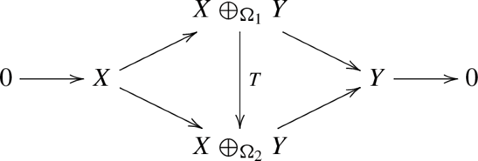
Let us check that the two definitions are equivalent.

The operator $\tau =\begin{pmatrix} Id &{}\quad -L \\ 0 &{}\quad Id \end{pmatrix}$ makes the diagram

commute and is a G-operator since

$$\begin{aligned} \begin{pmatrix} u(g) &{}\quad d_2(g) \\ 0 &{}\quad v(g) \end{pmatrix} \begin{pmatrix} Id &{}\quad -L \\ 0 &{}\quad Id \end{pmatrix} = \begin{pmatrix} Id &{}\quad -L \\ 0 &{}\quad Id \end{pmatrix} \begin{pmatrix} u(g) &{}\quad d_1(g) \\ 0 &{}\quad v(g) \end{pmatrix} \end{aligned}$$

because $d_2 - d_1 = [u, L, v]$. Finally, $\tau$ can be extended to a G-operator $T: X\oplus _{\Omega _1} Y \longrightarrow X\oplus _{\Omega _2} Y$ by density: set $(\omega , y) = \lim (\omega _n, \delta _n)$ and define $T(\omega , y)= \lim \tau (\omega _n, \delta _n)$. Since both actions are continuous, $\lambda _2 T(\omega , y)= \lambda _2 \lim \tau (\omega _n,\delta _n) = \lim \lambda _2 \tau (\omega _n,\delta _n) = \lim \tau \lambda _1 (\omega _n,\delta _n)= T\lambda _1 \lim (\omega _n,\delta _n) = T \lambda _1 (\omega , y)$. The other implication is easy: the existence of T implies the equivalence of the exact sequences in the category of Banach spaces, so that $\Omega _1-\Omega _2$ is boundedly equivalent to some L. Furthermore $T(X \oplus _{\Omega _1} \Delta ) \subseteq X \oplus _{\Omega _2} \Delta$, defining by restriction a G-operator $\tau$ as above, which is equivalent to saying that $d_2-d_1=[u,L,v]$.

Thus, there is a vector space structure on the set of pairs $(\Omega , d)$ (defined on the same $\Delta )$ given by $(\Omega _1, d_1) + (\Omega _2, d_2) = (\Omega _1+ \Omega _2, d_1 + d_2)$ and $\lambda (\Omega , d) = (\lambda \Omega , \lambda d_1)$. The zero element is the class of trivial sequences:

Definition 10.2

We will say that $(\Omega , d)$ is G-trivial, or that it G-splits, if $(\Omega , d)\simeq (0,0)$. This occurs if and only if there is a linear map L such that $\Omega - L$ is bounded and $d = -[u,L,v]$.

Proposition 10.3

Every quasilinear map $\Omega : \Delta \curvearrowright X$ defining a G-sequence $0\rightarrow X \rightarrow X\oplus _\Omega Y \rightarrow Y \rightarrow 0$ of G-spaces, is a linear perturbation of a G-centralizer (possibly with a larger target space). Furthermore the G-centralizer may be chosen so that its associated G-sequence with diagonal action is G-equivalent to the original G-sequence associated to $\Omega$.

Proof

Let $0\rightarrow X\rightarrow Z\rightarrow Y\rightarrow 0$ be an exact sequence of G-spaces. Set $\Sigma = Z$ as the ambient space equipped with $\lambda (g)$ as the extension of u(g). Any homogeneous bounded selection B for the quotient map: $B: Y\rightarrow Z$ is a G-centralizer generating the same sequence; in particular, writing $Z=X\oplus _\Omega Y$ so that $\lambda (g)= \left( \begin{array}{cc} u(g) &{}\quad d(g) \\ 0 &{}\quad v(g) \\ \end{array} \right)$ and then setting $\Omega _0 y= (\Omega y, y)$, then $\Omega _0$ is a G-centralizer, since the associated bounded action given by the diagonal maps $\lambda _0(g)= \left( \begin{array}{cc} \lambda (g) &{}\quad 0 \\ 0 &{}\quad v(g) \\ \end{array} \right)$ are uniformly bounded on $X \oplus _{\Omega _0} Y$: observe that $((\omega , y), y')\in X \oplus _{\Omega _0} Y$ exactly occurs when $(\omega , y) - \Omega _0 y' = (\omega - \Omega y', y - y') \in X$, which yields $y=y'$. Now:

$$\begin{aligned} \Vert \lambda _0(g)((\omega ,y), y)\Vert _{\Omega _0}= & {} \Vert (\lambda (g)(\omega , y), v(g)y)\Vert _{\Omega _0}\\= & {} \Vert (u(g)\omega + d(g) y, v(g) y)- (\Omega v(g)y, v(g)y)\Vert _\Omega + \Vert v(g)y\Vert _Y\\= & {} \Vert (u(g)\omega + d(g) y - \Omega v(g)y, 0)\Vert _\Omega + \Vert v(g)y\Vert _Y\\= & {} \Vert u(g)\omega + d(g) y - \Omega v(g)y\Vert _X + \Vert v(g)y\Vert _Y\\= & {} \Vert \lambda (g)(\omega , y)\Vert _\Omega \\\le & {} \Vert \lambda (g)\Vert \Vert (\omega , y)\Vert _\Omega \\= & {} \Vert \lambda (g)\Vert \Vert ((\omega , y), y)\Vert _{\Omega _0}. \end{aligned}$$

We perform the standard pushout from Lemma 3.3 to get $\xi \Omega _0 = \sigma \Omega + {\mathcal {L}}$. Note that by the comments after Lemma 3.3, $\xi \Omega _0$ is also a G-centralizer, with values in Z, defining the same exact sequence, and therefore $\sigma \Omega$ is a linear perturbation of a G-centralizer possibly with a larger target space. Finally, we note that $\sigma \Omega$ defines the same exact sequence of G-spaces as $\Omega$ (although formally one would have to replace d(g) by $\sigma d(g)$ to take values in the larger target space).

Now we show G-equivalence. Just to avoid misunderstandings: observe that when we combine the equality $\xi \Omega _0 = \sigma \Omega + {\mathcal {L}}$ of Lemma 3.3 with Definition 10.1, one has to set ${\mathcal {L}}= -L$ to get $T = \left( \begin{array}{cc} Id &{}\quad - L \\ 0 &{}\quad Id \\ \end{array} \right)$ as in the commuting diagram appearing in the description of Definition 10.1:

It only remains to see that T is a G-operator, i.e. to show that in $X\oplus _{\xi \Omega _0} Y$ the following holds:

$$\begin{aligned} (u(g)\omega -u(g) Ly, v(g) y)= & {} \left( \begin{array}{cc} u(g) &{}\quad 0 \\ 0 &{}\quad v(g) \\ \end{array} \right) \left( \begin{array}{cc} Id &{}\quad -L \\ 0 &{} \quad Id \\ \end{array} \right) \left( \begin{array}{c} \omega \\ y \\ \end{array} \right) \\= & {} \left( \begin{array}{cc} Id &{}\quad -L \\ 0 &{}\quad Id \\ \end{array} \right) \left( \begin{array}{cc} u(g) &{}\quad \sigma d(g) \\ 0 &{}\quad v(g) \\ \end{array} \right) \left( \begin{array}{c} \omega \\ y \\ \end{array} \right) \\= & {} (u(g)\omega + \sigma d(g)y - Lv(g)y, v(g) y)\end{aligned}$$

namely, $u(g)Ly = -\sigma d(g)y + Lv(g)y$ or, which is the same, $\sigma d(g)= -[u(g),L,v(g)]$.

To prove this equality, recall from the proof of Lemma 3.3 that $L(y)=-{\mathcal {L}}(y)=[-(\ell y,y), \ell y]$, where $\ell$ is linear so that $\Omega -\ell$ takes values in X. Therefore, and using the notation of Lemma 3.3,

$$\begin{aligned}{}[u(g),L,v(g)]y= & {} {\overline{u}}(g)\big (-(\ell y,y),\ell y\big ) -\big (-(\ell v(g)y, v(g)y),\ell v(g)y\big ) \\= & {} \big (-\lambda (g)(\ell y,y),u(g)\ell y\big ) -\big (-(\ell v(g)y, v(g)y),\ell v(g)y\big ) \\= & {} \big (-(u(g)\ell y+d(g)y,v(g)y),u(g)\ell y\big ) \\ {}{} & {} +\big ((\ell v(g)y, v(g)y),-\ell v(g)y\big ) \\= & {} \big ((-[u(g),\ell ,v(g)]-d(g))(y),0), [u(g),\ell ,v(g)](y)\big ) \\= & {} \big ( 0, -d(g)y \big ) \end{aligned}$$

The last line is due to the definition of the pushout ${\text {PO}}$ (where the computation takes place) as a quotient by a diagonal subspace of the form $\{([x,0],-x), x \in X\}$, together with the fact that the quantity $([u(g),\ell ,v(g)]+d(g))y$ belongs to X (because both $\Omega -\ell$ and $[u(g),\Omega ,v(g)]+d(g)$ take values in X). To conclude it is enough to remember from the definition of the embedding of $\Sigma$ in ${\text {PO}}$ that $\sigma d(g)y=(0,d(g)y)$. $\square$

We now give two easy lemmas that will help us simplify some proofs later on.

Lemma 10.4

Let $0\rightarrow X \rightarrow X\oplus _\Omega Y \rightarrow Y \rightarrow 0$ be a trivial exact sequence $(\Omega , d)$ of G-spaces. If $L: \Delta \curvearrowright X$ is any linear map for which $\Omega - L: \Delta \rightarrow X$ is bounded, then $d(g) + [u(g), L, v(g)]$ is a uniformly bounded family of operators.

Proof

$d(g)+[u(g),L,v(g)]= (d(g)+[u(g),\Omega ,v(g)]) + [u(g),L-\Omega , v(g)]$ and both terms of the sum are uniformly bounded. $\square$

Lemma 10.5

If $B:Y\rightarrow X$ is a bounded map with associated derivation d then $(B, d)\simeq (0,d)$

Proof

It is clear that the formal identity map $X\oplus _B Y \rightarrow X\oplus Y$ is a G-operator.$\square$

A warning is perhaps judicious here: sometimes, quasilinear maps $\Omega : Y\curvearrowright X$ are bounded maps $Y\rightarrow \Sigma$ but that does not imply that $\Omega$ is equivalent to 0, let alone $(\Omega , d)\simeq (0,d)$: beware that if $\Omega$ is not bounded with respect to the $\Vert .\Vert _X$-norm, no identity map $X\oplus _\Omega Y\rightarrow X\oplus Y$ exists. G-splitting admits natural characterizations, similar to those in the Banach space category.

Proposition 10.6

Consider an exact sequence $(\Omega , d)$ of G-spaces $0 \rightarrow X \rightarrow Z \rightarrow Y \rightarrow 0$. The following assertions are equivalent:

• (i) The sequence G-splits.

• (ii) The quotient map admits a linear continuous G-lifting.

• (iii) X admits a G-invariant complement.

• (iv) X is G-complemented in Z.

Proof

A few hints will suffice: If L is a G-lifting then L[Y] is a G-complement of X; $L(y)=(\ell y, y)$ with $\ell -\Omega$ bounded and $d = -[u, \ell , v]$ is a derivation.$\square$

In complete analogy with classical Banach space homology, we can define now the vector space ${\text {Ext}}_G(Y,X)$ of G-equivalence classes of pairs $(\Omega , d)$. Our next result presents “group" versions of two theorems of Cabello: the first one [3, Cor. 2] asserts that an exact sequence of $L_\infty$-modules that algebraically splits also splits topologically; the second and [4, Theorem 1] says that when $p\ne q$ the only exact sequence of quasi-Banach $L_\infty$-modules $0\rightarrow L_q\rightarrow Z\rightarrow L_p\rightarrow 0$ is the trivial one while, as it is well known [7, Proposition 5.2.20], ${\text {Ext}}(L_p, L_q)\ne 0$ as Banach spaces.

Theorem 10.7

Let G be a group and let $0\rightarrow X \rightarrow X\oplus _\Omega Y \rightarrow Y \rightarrow 0$ be a trivial exact sequence of G-spaces. If G is amenable and X is a G-ultrasummand then the sequence G-splits.

Proof

Let $(\Omega , d)$ describe the exact sequence above and assume that $\Omega$ is trivial. We use Proposition 10.3 to obtain a G-centralizer $\Omega _0$ so that $(\Omega , d) \simeq (\Omega _0, 0)$. Since we are told that $(\Omega _0, 0)$ splits, Lemma 10.4 yields a linear map $\tau :\Delta \rightarrow \Sigma$ for which $\Omega _0 - \tau : \Delta \rightarrow X$ is bounded and $(\Omega _0, 0)\simeq (\Omega _0 - \tau , [u,\tau , v]) \simeq (0, [u, \tau , v])$ by Lemma 10.5. Thus, the proof can be reduced to proving that, under the hypothesis of the theorem, if $B:\Delta \rightarrow X$ is a bounded map then $(B, d)\simeq (B, 0)$ for whatever d. Let us call $X\oplus _B^d Y$ and $X\oplus _B^0 Y$ the spaces endowed with the actions induced by, respectively, the derivations d and 0. Recall from Lemma 10.4 that $\{d(g)\}_{g\in G}$ is a uniformly bounded family of operators, and therefore we can form the operator

$$\begin{aligned} My =P\left( \int _{g \in G} u(g^{-1})d(g)y\; d\mu (g)\right) \end{aligned}$$

where $P: X^{**} \rightarrow X$ is a G-projection. Let us show that the map $R=\begin{pmatrix} Id &{}\quad M\\ 0 &{}\quad Id \end{pmatrix}$ is a G-operator making the diagram

commute. The only part that is not evident, that R is a G-operator, means

$$\begin{aligned} \left( \begin{array}{cc} u &{}\quad 0 \\ 0 &{}\quad v \\ \end{array} \right) R = R \left( \begin{array}{cc} u &{}\quad d \\ 0 &{}\quad v\\ \end{array} \right) \end{aligned}$$

namely $u(g)M = d(g)+ Mv(g)$, i.e., $d=[u,M,v]$. We show this:

$$\begin{aligned} u(g')My= & {} u(g')P\left( \int _{g \in G} u(g^{-1})d(g)y\; d\mu (g)\right) \\= & {} P\left( \int _{g \in G} u(g'g^{-1})d(g)y \; d\mu (g)\right) \\ \end{aligned}$$

Call $g'g^{-1} = h^{-1}$ so that $g=hg'$ and thus

$$\begin{aligned}= & {} P\left( \int _{h \in G} u(h^{-1})d(hg') y\; d\mu (h)\right) \\= & {} P\left( \int _{h \in G} u(h^{-1})(u(h)d(g') + d(h)v(g')) y\; d\mu (h)\right) \\= & {} d(g')y + P\left( \int _{h \in G}u(h^{-1})d(h)v(g')) y\; d\mu (h)\right) \\= & {} d(g')y + Mv(g')y. \end{aligned}$$

$\square$

Corollary 10.8

Let G be a group. Let $0\rightarrow X \rightarrow X\oplus _\Omega Y \rightarrow Y \rightarrow 0$ and $0\rightarrow X \rightarrow X\oplus _\Phi Y \rightarrow Y \rightarrow 0$ be exact sequences $(\Omega , d)$, $(\Phi , d')$ of G-spaces. If G is amenable and X is a G-ultrasummand then

$$\begin{aligned} (\Omega , d) \simeq (\Phi , d') \Longleftrightarrow \Omega \sim \Phi . \end{aligned}$$

It will help us at this point to use the classical terminology, and call inner a derivation for which there exists a bounded linear map $A: Y \rightarrow X$ such that $d = [u,A,v]$.

Remark 10.9

Note that $(\Omega , d_1) \simeq (\Omega , d_2)$ if and only if $d_1 -d_2$ is inner.

To see this, just apply Definition 10.1 with $\Omega _1=\Omega _2=\Omega$ to obtain a linear map $A: \Delta \curvearrowright X$ such that $d_1(g)-d_2(g)=[u(g),A,v(g)]$, and $\Omega -\Omega +A$ bounded, i.e. A is a bounded operator, which by extension may be assumed to be defined on the whole of Y.

Both hypotheses in Corollary 10.8 are necessary. (a) The amenability of G is necessary, because while ${\text {Ext}}(\ell _2(T), \ell _2(T))=0$, we have that ${\text {Ext}}_{\textrm{Aut}(T)}(\ell _2(T), \ell _2(T))\ne 0$. Indeed, see the end of Section 3: the sequence

$$\begin{aligned} 0\rightarrow \ell _2(T)\rightarrow \ell _2(T) \oplus _L \ell _2(T)\rightarrow \ell _2(T)\rightarrow 0, \end{aligned}$$

where $\ell _2(T)$ is equipped with the action u and $\ell _2(T) \oplus _L \ell _2(T)$ is equipped with the diagonal action, does not $\textrm{Aut}(T)$-splits. Otherwise we would have $(L,0) \simeq (0,0)$, which means by definition that $L-\ell$ is bounded and $[u,\ell ,u]=0$ for some linear map $\ell$. In other words, L would be boundedly equivalent to an $\textrm{Aut}(T)$-equivariant map $\ell$, a contradiction with the second part of Proposition 3.11. (b) The G-ultrasummand character of X is necessary, because ${\text {Ext}}({\mathbb {R}}, c_0)=0$ but we will show in Sect. 11.3 that ${\text {Ext}}_{2^{<\omega }}({\mathbb {R}}, c_0)\ne 0$.

If we put together Theorem 10.7 and the result of Cabello mentioned before it we almost get a contradiction: after all, the group ${\mathcal {U}}$ of units of the $L_\infty$-module structure is Abelian (hence amenable) and (for $1<p<\infty$) $L_p$ spaces are reflexive. Let us however carefully spell what these two results together actually imply: no non-trivial element of $\textrm{Ext}(L_p,L_q)$ can be compatible with the canonical actions of ${\mathcal {U}}$ on these two spaces.

A significant consequence of Theorem 10.7 is the following kind of uniqueness result for the possible derivation associated to fixed actions u and v.

Corollary 10.10

Assume that G is an amenable group, Y and X are G-spaces with X a G-ultrasummand and $\Omega : Y\curvearrowright X$ is a quasilinear map. All compatible actions of G on $X \oplus _\Omega Y$ are conjugate; namely, given two such actions $\lambda _1, \lambda _2$ there is $A \in {\mathfrak {L}}(Y,X)$ such that for all $g \in G$,

$$\begin{aligned} \lambda _2(g)=\begin{pmatrix} Id &{}\quad A \\ 0 &{}\quad Id \end{pmatrix} \lambda _1(g) \begin{pmatrix} Id &{}\quad -A \\ 0 &{}\quad Id \end{pmatrix}. \end{aligned}$$

Proof

Since the two exact sequences of Banach spaces are equivalent, Theorem 10.7 implies that they are equivalent in the G-space setting, i.e. $(\Omega ,d_1) \simeq (\Omega ,d_2)$. By Remark 10.9, $d_1-d_2$ is therefore inner, so pick A such that $d_1(g)-d_2(g)=[u(g),A,v(g)]$. $\square$

In the particular case of a direct sum of two copies of a Hilbert space H on which $u=v$ is a unitary representation, note that compatible actions of G are represented by triangular matrices of the form $\lambda (g)=\begin{pmatrix} u(g) &{}\quad d(g) \\ 0 &{}\quad u(g) \end{pmatrix}$, where d(g) is uniformly bounded. If G is amenable then Corollary 10.10 implies that such an action is conjugate to the diagonal action associated to u, i.e.

$$\begin{aligned} \lambda (g)=\begin{pmatrix} u(g) &{}\quad d(g) \\ 0 &{}\quad u(g) \end{pmatrix}=\begin{pmatrix} Id &{}\quad A \\ 0 &{}\quad Id \end{pmatrix} \begin{pmatrix} u(g) &{}\quad 0 \\ 0 &{}\quad u(g) \end{pmatrix} \begin{pmatrix} Id &{}\quad -A \\ 0 &{}\quad Id \end{pmatrix}. \end{aligned}$$

Unravelling this expression, we obtain that $d(g)=[A,u(g)]$ is inner.

It is a well known fact that a bounded triangular representation is unitarizable (i.e. similar to a unitary representation) if and only if the corresponding derivation is inner (see the beginning of [28] Section 3 for a full statement and a proof). We previously recalled that bounded representations of amenable groups are unitarizable [25, 26]. So, under amenability of G, Corollary 10.10 may be seen as a generalization, to the context of general twisted sums of G-spaces, of the characterization of unitarizability by inner derivations in the context of direct sums of two Hilbert spaces.

11 Variations and Comments

This final section contains a miscellanea of results and problems connected with the ideas in this paper.

11.1 From Uniformly Bounded Extensions to Actions

The following situation was mentioned in the abstract: to which extent the existence of a uniformly bounded family of operators on a twisted sum space compatible with a couple of actions on the subspace and the quotient space induces an action on the twisted sum. We have:

Proposition 11.1

Let $\Omega : Y\curvearrowright X$ be quasi-linear between two G-spaces. Assume that there is a uniformly bounded family of operators $(T_g)_{g\in G}$ such that each $T_g: X \oplus _\Omega Y\rightarrow X \oplus _\Omega Y$ forms a commutative diagram

If G is an amenable group and X is a G-ultrasummand then there is a compatible action of G on $X\oplus _\Omega Y$.

Proof

Each operator $T_g$ has the form $T_g = \left( \begin{array}{cc} u(g) &{}\quad \tau _g \\ 0 &{}\quad v(g) \\ \end{array} \right) .$ We may assume wlog that $\tau _{e}=0$ by simply replacing the family $(T_g)_g$ by $(S_g)_g$ with $S_g= T_g + Id - T_e$. Since $T_{g}^{-1}$ has to have the form $\left( \begin{array}{cc} u(g)^{-1} &{}\quad b(g) \\ 0 &{}\quad v(g)^{-1} \\ \end{array} \right)$, from $T_{g}^{-1} T_g = Id$ and $\tau _e=0$ we obtain $b(g)= - u(g^{-1})\tau _g v(g^{-1})$, so that $T_{g}^{-1} = \left( \begin{array}{cc} u(g^{-1}) &{}\quad - u(g^{-1})\tau _g v(g^{-1} ) \\ 0 &{}\quad v(g^{-1}) \\ \end{array} \right)$. Now, it may well happen that $T_g^{-1}$ is not $T_{g^{-1}}$. To amend this, what we claim is that $\sup _g \Vert (T_g)^{-1}\Vert < \infty$: this is consequence of $\Vert (T_g)^{-1}(x,0)\Vert \le \Vert u(g^{-1})x\Vert$ and

$$\begin{aligned}{} & {} \sup _{\Vert x\Vert \le 1} \Vert (T_g)^{-1}(\Omega x, x)\Vert \\{} & {} \quad = \sup _{\Vert x\Vert \le 1} \Vert u(g^{-1})\Omega x - u(g^{-1})\tau _g v(g^{-1}) x - \Omega v(g^{-1})x\Vert +\Vert v(g^{-1})x\Vert \\{} & {} \quad \le \Vert u(g^{-1})\Vert \sup _{\Vert x\Vert \le 1} \Vert \Omega x - \tau _g v(g^{-1}) x - u(g)\Omega v(g^{-1})x\Vert +\Vert v(g^{-1})\\{} & {} \quad \le \Vert u(g^{-1})\Vert \sup _{\Vert y\Vert \le \Vert v(g^{-1})\Vert } \Vert \Omega v(g)y - \tau _g y - u(g)\Omega y\Vert +\Vert v(g^{-1})\Vert \\{} & {} \quad \le \Vert u(g^{-1})\Vert \sup _{\Vert y\Vert \le \Vert v(g^{-1})\Vert } \Vert T_g( \Omega y, y)) \Vert +\Vert v(g^{-1})\Vert \\{} & {} \quad \le \Vert u(g^{-1})\Vert (\Vert T_g\Vert +1) \Vert v(g^{-1})\Vert \end{aligned}$$

This is enough: for any pair $g, g^{-1}\in G$, pick one of them to remain $T_g$ and replace $T_{g^{-1}}$ by $T_g^{-1}$. Thus, from now on we assume that $(T_g)^{-1}=T_{g^{-1}}$ and thus, what is more important to us, that

$$\begin{aligned} \tau _{g^{-1}} = - u(g^{-1}) \tau _g v(g^{-1}). \end{aligned}$$

The family $\{ [u(g),\Omega , v(g)] + \tau _g\}_{g\in G}$ is uniformly bounded since

$$\begin{aligned} \left( \begin{array}{cc} u(g) &{}\quad \tau _g \\ 0 &{}\quad v(g) \\ \end{array} \right) \left( \begin{array}{c} \Omega y \\ y \\ \end{array} \right) = (u(g)\Omega y + \tau _g y, v(g)) \end{aligned}$$

is a uniformly bounded family and $\Vert (u(g)\Omega y + \tau _g y, v(g))\Vert = \Vert u(g)\Omega y + \tau _g y - \Omega v(g)\Vert + \Vert v(g)\Vert$. Thus, both

• $\left( \begin{array}{cc} u(gh) &{} \quad \tau _{gh} \\ 0 &{} \quad v(gh) \\ \end{array} \right) _{g,h}$

• $\left( \begin{array}{cc} u(g) &{}\quad \tau _{g} \\ 0 &{} \quad v(g) \\ \end{array} \right) _g\left( \begin{array}{cc} u(h) &{}\quad \tau _{h} \\ 0 &{}\quad v(h) \\ \end{array} \right) _h = \left( \begin{array}{cc} u(gh) &{}\quad u(g)\tau _h + \tau _g v(h)\\ 0 &{}\quad v(gh) \\ \end{array} \right) _{g,h}$

define uniformly bounded families of operators, hence $\left( \begin{array}{cc} 0 &{}\quad u(g)\tau _h + \tau _g v(h) - \tau _{gh} \\ 0 &{}\quad 0 \\ \end{array} \right) _{g,h}$ is also a uniformly bounded family. Since

$$\begin{aligned} \left( \begin{array}{cc} 0&{} \quad u(g)\tau _h + \tau _g v(h) - \tau _{gh}\\ 0 &{}\quad 0 \\ \end{array} \right) \left( \begin{array}{c} \Omega y \\ y \\ \end{array} \right) = ((u(g)\tau _h + \tau _g v(h) - \tau _{gh}) y, 0) \end{aligned}$$

and $\Vert (u(g)\tau _h + \tau _g v(h) - \tau _{gh}) y, 0)\Vert _{X\oplus _\Omega Y}= \Vert (u(g)\tau _h + \tau _g v(h) - \tau _{gh}) y\Vert _X$ it turns out that the family $\{u(g)\tau _h + \tau _g v(h) - \tau _{gh}\}_{g,h\in G}$ is uniformly bounded. Set gh instead of g and $h^{-1}$ instead of h and get that also $\{u(gh)\tau _{h^{-1}} + \tau _{gh} v(h^{-1}) - \tau _{g}\}_{g,h\in G}$ is uniformly bounded. Hence,

$$\begin{aligned} \{u(gh)\tau _{h^-1} + \tau _{gh} v(h^{-1})\}_{h\in G} \end{aligned}$$

is a uniformly bounded family and we can therefore define

$$\begin{aligned} d(g)=P\left( \int _{h \in G} (u(gh)\tau _{h^{-1}}+ \tau _{gh}v(h^{-1}) )d\mu \right) , \end{aligned}$$

where P is a G-operator $X^{**} \rightarrow X$. Let us check that d is a derivation: given g, k in G, since

$$\begin{aligned} u(gkh)\tau _{h^{-1}k^{-1}}v(k) + u(g)\tau _{kh} v(h^{-1})= & {} u(g)\left( u(kh)\tau _{h^{-1}k^{-1}} + \tau _{kh} v(h^{-1}k^{-1}) \right) v(k)\\ {}= & {} 0 \end{aligned}$$

we have

$$\begin{aligned} d(gk)= & {} P\left( \int _{h \in G} u(gkh)\tau _{h^{-1}}+ \tau _{gkh}v(h^{-1}) d\mu \right) \\= & {} P\left( \int _{h \in G} u(gkh) \tau _{h^{-1}} + \tau _{gkh} v(h^{-1}) + u(gkh)\tau _{h^{-1}k^{-1}}v(k) + u(g)\tau _{kh} v(h^{-1}) d\mu \right) \\= & {} P\left( \int _{h \in G} u(gkh) \tau _{h^{-1}} + u(g)\tau _{kh} v(h^{-1}) d\mu + \int _{h \in G} \tau _{gkh} v(h^{-1})\right. \\{} & {} +\left. u(gkh)\tau _{h^{-1}k^{-1}}v(k) d\mu \right) \\= & {} u(g)P\left( \int _{h \in G} u(kh) \tau _{h^{-1}} + \tau _{kh} v(h^{-1}) d\mu \right) \\{} & {} + \left( \int _{h \in G} u(gkh)\tau _{h^{-1}k^{-1}} + \tau _{gkh} v(h^{-1}k^{-1}) d\mu \right) v(k) \\= & {} u(g) d(k) + \left( \int _{h \in G} u(gh)\tau _{h^{-1}} + \tau _{gh} v(h^{-1}) d\mu \right) v(k) \\= & {} u(g)d(k) + d(g) v(k).\end{aligned}$$

Finally, d is an $\Omega$-derivation, i.e., $\{[u(g), \Omega , v(g)] + d(g)\}_g$ is uniformly bounded: on one hand, the family $[u(g), \Omega , v(g)] + \tau _g$ is uniformly bounded and on the other $(d(g) - \tau _g )$ too because $\{u(gh)\tau _{h^{-1}} + \tau _{gh} v(h^{-1}) - \tau _{g}\}_{g,h\in G}$ is uniformly bounded and P is a G-operator. Thus $[u(g), \Omega , v(g)] + d(g) = [u(g), \Omega , v(g)] + \tau _g - \tau _g + d(g)$ defines a uniformly bounded family.$\square$

Let us conclude with a comment about the hypothesis of Proposition 11.1. Observe that the existence of an operator T making a commutative diagram

is equivalent to the existence of a linear map $L:\Delta \rightarrow \Sigma$ such that $u\Omega - \Omega v - L: \Delta \longrightarrow X$ and $\Vert u\Omega - \Omega v - L\Vert <\infty$. In this way, if we denote $\texttt {Lin}(\Delta ,\Sigma )$ the space of all linear maps (continuous or not) between $\Delta$ and $\Sigma$, the hypothesis of Proposition 11.1 can be reformulated as $\sup _{g\in G} \text {dist}\left( u(g)\Omega - \Omega v(g), \texttt {Lin}(\Delta ,\Sigma )\right) <\infty$. The proof could have been plotted this way showing how to replace the original family $(T_g)_g$ by a new family $(s_g)_g$ such that $\sup _{g\in G} \Vert s_g\Vert \sim \sup _{g\in G} \Vert u(g)\Vert ,\Vert v(g)\Vert$. A simple example in [15] shows that in a general commutative diagram formed by two exact sequences and three operators u, T, v the norm of T is not necessarily bounded by those of u and v.

11.2 Complex Structures

We now answer a question about complex structures on real twisted sum spaces posed in [17, around Corollary 2.2].

Proposition 11.2

Let X, Y be Banach spaces admitting complex structures u, v and let $\Omega : Y\curvearrowright X$ be a quasilinear map. If there exists a bounded operator T on $X \oplus _\Omega Y$ yielding a commutative diagram

then $X\oplus _\Omega Y$ admits a complex structure.

Proof

We use the abelian, hence amenable, group $G=\{i,-1,-i,1\}$ through the action $i\rightarrow u, 1\rightarrow id, -i\rightarrow -u, -1 \rightarrow -id$ on X and $i\rightarrow v, 1\rightarrow id, -i\rightarrow -v, -1 \rightarrow -id$ on Y. With this we may apply a simple version of Proposition 11.1, for which no G-complementation is required since one performs just a finite average (i.e. P is removed in the definition of d(g)). Then $J=\begin{pmatrix} u &{}\quad d(i) \\ 0 &{}\quad v\end{pmatrix}$ is a complex structure. The value of d(i), which is $\frac{1}{2}(\tau + u \tau v)$, may be computed unravelling the formula in Proposition 11.1. More directly: it is an immediate computation that the associated $J=\begin{pmatrix} u &{}\quad \frac{1}{2}(\tau +u\tau v) \\ 0 &{}\quad v\end{pmatrix}$ has square $-Id$, and the boundedness of J may be checked as follows. By boundedness of T, $[u,\Omega ,v]+\tau =u\Omega -\Omega v+\tau$ is bounded. Composing on the left by u and on the right by v, we obtain that $-\Omega v +u\Omega +u\tau v=[u,\Omega ,v]+u\tau v$ is bounded, which means that $R:=\begin{pmatrix} u &{}\quad u \tau v \\ 0 &{}\quad v \end{pmatrix}$ is bounded as well. Finally $J=\frac{1}{2}(T+R)$ is bounded. $\square$

This proof shows that complex structures exist in $X\oplus _\Omega Y$ as long as $[u, \Omega , v]$ is the sum of a bounded and of a linear map. The result had been proved in [17, Corollary 2.2] assuming that $[u,\Omega , v]$ was either bounded or linear.

11.3 Actions of the Cantor Group $2^\omega$ and of $2^{<\omega }$

The goal of this Section is to provide new natural examples and showing that the G-ultrasummand character of X is necessary in Theorem 10.7. The Cantor group is the group of units of $\ell _\infty$ and thus $2^\omega$-centralizers are just $\ell _\infty$-centralizers. Its diagonal action on $\ell _\infty$ restricted to $c_0$ is again the diagonal action, and thus it generates an action on $\ell _\infty /c_0$. We do not have any reasonable idea about a linear derivation $d: \ell _\infty /c_0\rightarrow c_0$ of the Cantor group. The subgroup $2^{<\omega }$ of elements of $2^\omega$ that are eventually 1 is much more manageable. The space c is the living example that $2^{<\omega }$-groups are not $2^{\omega }$-groups. The natural diagonal action of $2^{<\omega }$ on c and $c_0$, who is therefore a $2^{<\omega }$-subspace, induces the identity action on the quotient ${\mathbb {R}}$. This implies that the exact sequence $0\rightarrow c_0 \rightarrow c \rightarrow {\mathbb {R}}\rightarrow 0$ of $2^{<\omega }$-spaces, which splits as a Banach space sequence, does not split as a $2^{<\omega }$-sequence since no $2^{<\omega }$-lifting ${\mathbb {R}}\rightarrow c$ is possible. Thus, ${\text {Ext}}_{2^{<\omega }}({\mathbb {R}}, c_0)\ne 0$, which shows that G-complementation is necessary in Theorem 10.7. Observe that Corollary 10.10 does not apply and therefore we do not know the general form of an action of $2^{<\omega }$ on c. The map $d(g): {\mathbb {R}}\rightarrow c_0$ is $d(g)(r) = -2r \sum _{g_i = - 1} e_i$ is a linear derivation on $2^{<\omega }$ and the triangular action on c has the form $\lambda (g)= \begin{pmatrix} u(g) &{}\quad d(g) \\ 0 &{}\quad Id_{\mathbb {R}}\end{pmatrix}$ with u the diagonal. In the spirit of Definition 10.1, note that d can also be written as $d=[u,L,v]$ where $L: {\mathbb {R}}\rightarrow c$ is defined by $L(r)=(r,r,\ldots )$, so we can also write equivalently that $c_0 \oplus _L {\mathbb {R}}$ equipped with the diagonal action is not $2^{<\omega }$-trivial. Each element x of ${\mathfrak {L}}({\mathbb {R}}, c)=c$ defines an $2^{<\omega }$-centralizer in the form $\Omega (1)=x$ but none defines an equivariant $2^{<\omega }$-centralizer since $u(g)x - x =0$ for all $g\in G$ is impossible. All this was based on some ideas of [1], where an example of an SOT-discrete bounded group of operators on $c_0$ without discrete orbits was provided; the relation with twisted sums was not observed there.

There is a general formulation for this situation: let X be a separable Banach space that we write as $X=\overline{\bigcup _n F_n}$ for an increasing sequence of finite dimensional spaces $F_n$. The space $c_0({\mathbb {N}}, F_n)$ admits a natural “diagonal" action $g(f_n)= (g(n)f_n)$ that naturally extends to the space $c_X(F_n)= \{(f_n): \exists \lim f_n\}$. What is interesting here is that the exact sequence $0 \rightarrow c_0({\mathbb {N}}, F_n) \rightarrow c_X({\mathbb {N}}, F_n) {\mathop {\rightarrow }\limits ^{\lim }}X \rightarrow 0$ splits if and only if X has the Bounded Approximation Property [7, Chapter 5] although it never $2^{<\omega }$-splits since the action induced on X is the identity.

The difficulty of obtaining derivations $\ell _\infty /c_0\rightarrow c_0$ for $2^\omega$ can be confronted with how easily one obtains derivations for $2^{<\omega }$ on the subspace $c_0({\mathfrak {c}})$ of $\ell _\infty /c_0$ (here ${\mathfrak {c}}$ is the cardinal of the continuum). Consider to this end that the Nakamura-Kakutani (see [7, 2.2.10]) sequences $0 \longrightarrow c_0 \longrightarrow C(\Delta _{{\mathcal {A}}} ) \longrightarrow c_0(|{\mathcal {A}}|) \longrightarrow 0$ also provide natural examples of $2^{<\omega }$-centralizers: pick ${\mathcal {A}}$ an almost disjoint family of subsets of ${\mathbb {N}}$ (i.e., $|A\cap B|<\infty$ for all $A, B \in {\mathcal {A}}$) containing the singletons. The cardinal of the family must be $\aleph _1 \le |{\mathcal {A}}|\le {\mathfrak {c}}$ since when $|{\mathcal {A}}|=\aleph _0$ the sequence splits by Sobczyk’s theorem. We will assume without loss of generality that it is the continuum. Let $\Delta _{{\mathcal {A}}}$ be the one-point compactification of the locally compact space having ${\mathbb {N}}$ as isolated points and $A\in {\mathcal {A}}$ as the only accumulation point of $\{n: n\in A\}$. There is a natural action of $2^{<\omega }$ on $C(\Delta _{{\mathcal {A}}})$: $(gf)(n)= g(n)f(n)$ that yields the diagonal action on $c_0$ and induces the identity action on $c_{0}({\mathfrak {c}})$. Let $c_{00}({\mathfrak {c}})$ be the dense subspace of all finitely supported sequences. A quasilinear map $\Omega : c_{00}({\mathfrak {c}})\curvearrowright c_0$ corresponding to this sequence can be easily described: fix a well-order on ${\mathfrak {c}}$ and then for $x\in c_{00}({\mathfrak {c}})$ write it as $x=\sum \lambda _i e_i$ with the $e_i$ well ordered and define $\Omega ( \sum \lambda _i e_i) = \lambda _1 1_{A_1} + \lambda _2 1_{A_2 {\setminus } A_1} + \cdots + \lambda _n 1_{A_n {\setminus } (A_1\cup \dots A_{n-1})}$. This is a bounded map $c_{00}({\mathfrak {c}})\rightarrow \ell _\infty$ and therefore a $2^{<\omega }$-centralizer (with derivation 0). On the other hand, $C(\Delta _{{\mathcal {A}}})$ is a subspace of $\ell _\infty$ but the natural action of $2^\omega$ does not respect $C(\Delta _{{\mathcal {A}}})$.

11.4 Groups and Symmetries

To fix ideas, let us focus on ${\mathbb {N}}$ and $\ell _\infty$-centralizers (namely, $2^\omega$-centralizers) on Banach spaces with symmetric basis. A centralizer is symmetric if $\Vert (\Omega x)\sigma - \Omega (x\sigma )\Vert \le C \Vert x\Vert$ for every permutation $\sigma$ of ${\mathbb {N}}$. For instance $\textsf{KP}$ maps are symmetric. Symmetric centralizers live their own lives (see [4, 35]) and there is a great difference between working with symmetric and non-symmetric centralizers. But the ideas in the present paper allow us to explore the intermediate terrain between “centralizer" and “symmetric centralizer". Let Sym$({\mathbb {N}})$ be the group of permutations of ${\mathbb {N}}$ and let $\Theta$ be a subgroup. Consider the set $2^{\omega }_\Theta = 2^{\omega } \times \Theta$ with the group structure corresponding to the action $(g,\theta )(x) = g(x\theta )$ where $(x\theta )(n)= x(\theta (n))$. Symmetric centralizers correspond to $2^{\omega }_{ \texttt {Sym}({\mathbb {N}})}$-centralizers. Let now $(A_n)$ be a partition ${\mathbb {N}}=\cup A_n$ of ${\mathbb {N}}$ into finite sets, $A_n<A_{n+1}$, and let $\Theta$ be the group of permutations $\sigma$ of ${\mathbb {N}}$ such that $\sigma A_n = A_n$ for all n. It turns out that $2^{\omega }_{\Theta }$-centralizers can be useful too: as the authors of [12] dismayingly recall, the first author has frequently asked about “how many different" exact sequences $0\rightarrow \ell _1\rightarrow Z \rightarrow c_0\rightarrow 0$ exist. The same problem is addressed in [7]. Let us lodge the problem in the theory developed in this paper.

Proposition 11.3

Every non $2^{\omega }_{\Theta }$-trivial $2^{\omega }_{\Theta }$-centralizer $\ell _2\curvearrowright \ell _2$ generates a nontrivial exact sequence $0\rightarrow \ell _1\rightarrow X \rightarrow c_0\rightarrow 0$.

Proof

Let $\Omega : \ell _2\curvearrowright \ell _2$ be a $2^{\omega }_{\Theta }$-centralizer. This means that for the partition $(A_n)$ of ${\mathbb {N}}$ and every permutation $\sigma$ of ${\mathbb {N}}$ such that $\sigma A_n = A_n$ one has for every $x\in \ell _2$ that $(\Omega x)\sigma - \Omega (x\sigma )\in \ell _2$ and this family is uniformly bounded. In particular, if we decompose $\ell _2= \ell _2({\mathbb {N}}, \ell _2(A_n))$ then $\Omega |_{\ell _2(A_n)}\subset \ell _2(A_n)$. Being $2^{\omega }_{\Theta }$-trivial means that there is a linear map $L: \ell _2({\mathbb {N}}, \ell _2(A_n))\rightarrow \Sigma$ such that $\Omega - L: \ell _2({\mathbb {N}}, \ell _2(A_n))\longrightarrow \ell _2({\mathbb {N}}, \ell _2(A_n))$ and $(\Omega - L)|_{\ell _2(A_n)}$ is uniformly bounded. Thus, if $\Omega$ is not $2^{\omega }_{\Theta }$-trivial, the sequence

splits, but if $\sigma _n^{-1}$ denotes its splitting constant (namely, the infimum of those constants C for which there is a linear map $\ell _n: \ell _2(A_n)\rightarrow \ell _2(A_n)$ such that $\Vert \Omega |_{\ell _2(A_n)} - \ell _n\Vert \le C$) then $\lim \sigma _n =0$ since otherwise $\Omega$ would be $2^{\omega }_{\Theta }$-trivial. Some subsequence $(\sigma _{k(n)})_n\in \ell _{1/2}$, and we will shamelessly assume that it is $\sigma$. Let $D: c_0({\mathbb {N}}, \ell _2(A_n)) \rightarrow \ell _2({\mathbb {N}}, \ell _2(A_n))$ be the “diagonal" map $D((x_n))=(\sigma _n^{1/4} x_n)$. Form the commutative diagram

The lower sequence has $D \Omega D$ as associated quasilinear map and this it cannot split since otherwise the upper sequence would be $2^{\omega }_{\Theta }$-trivial: after all, since $(D \Omega D)|_{\ell _2(A_n)} (x) = \sigma _n^{1/2} \Omega x$ and thus if there is a sequence of linear maps $\ell _n: \ell _2(A_n)\rightarrow \ell _2(A_n)$ such that $\Vert D\Omega D|_{\ell _2(A_n) } - \ell _n\Vert \le M$ then the splitting constant of of $\Omega |_{\ell _2(A_n)}$ would be at most $M\sigma _n^{-1/2}$. To conclude, if $\jmath _n: \ell _2(A_n)\rightarrow \ell _1^{2^n}$ is a sequence of C-isomorphic embeddings then $(\jmath _n) D \Omega D (\jmath _n^*)$ is nontrivial by the local version of [7, Claim p.268]), and this produces a nontrivial sequence

$\square$

Even if $D\Omega D$ is a $2^\omega$-centralizer, $(\jmath _n) D \Omega D (\jmath _n^*)$ is not, and can never be, a $2^\omega$-centralizer: otherwise there would be a compatible action of $2^\omega$ on X and picking any extension $T: X\rightarrow {\mathbb {R}}$ of the sum functional $\ell _1\rightarrow {\mathbb {R}}$ we can form the $2^\omega$-invariant functional $\Lambda (x) = \int _{2^\omega } \varepsilon ^{-1}T(\varepsilon x) d\mu$. The road is now paved to define $Q: X\rightarrow \ell _1^{**}$ in the form $Q(x)(\varepsilon ) = \Lambda (\varepsilon x)$ for $\varepsilon$ an unit of $\ell _\infty$ and extend it linearly to a functional on $\ell _\infty$. Finally, compose with a $2^\omega$-projection $\ell _1^{**}\rightarrow \ell _1$. It is however perfectly reasonable to have a G-centralizer $\Omega$ and two operators $\alpha , \gamma$ so that $\alpha \Omega \gamma$ is a $G'$-centralizer for two different groups $G,G'$. Researchers willing to travel this road are advised to do so crossing through the horn gate of [12].

11.5 Additional Structures

Additional structures other than group structures may be considered on Banach spaces. See for example the work of Corrêa [20] on exact sequences of operator spaces and a solution to 3-space problem for OH spaces. It seems to be unknown whether a relevant theory of groups acting completely boundedly on extension sequences of operator spaces may be developed.

References

Antunes, L., Ferenczi, V., Grivaux, S., Rosendal, Ch.: Light groups of isomorphisms of Banach spaces and invariant LUR renormings. Pac. J. Math. 301(1), 31–54 (2019)
Bergh, J., Löfström, J.: Interpolation Spaces. An Introduction. Springer (1976)
Cabello Sánchez, F.: Nonlinear centralizers with values in \(L_0\). Nonlinear Anal. 88, 42–50 (2013)
Cabello Sánchez, F.: Nonlinear centralizers in homology. Math. Ann. 358, 779–798 (2014)
Cabello Sánchez, F.: There is no strictly singular centralizer on \(L_p\). Proc. Am. Math. Soc. 142, 949–955 (2014)
Cabello Sánchez, F.: The noncommutative Kalton–Peck spaces. J. Noncommun. Geom. 11, 1395–1412 (2017)
Cabello Sánchez, F., Castillo, J.M.F.: Homological Methods in Banach Space Theory. Cambridge Studies in Advanced Mathematics, vol. 203 (2023)
Cabello Sánchez, F., Castillo, J.M.F., Correa, W.H.G.: Higher order derivatives of analytic families of Banach spaces. Studia Math. (to appear). arXiv:1906.06677v2
Cabello Sánchez, F., Castillo, J.M.F., Kalton, N.J.: Complex interpolation and twisted twisted Hilbert spaces. Pac. J. Math. 276, 287–307 (2015)
Cabello Sánchez, F., Castillo, J.M.F., Suárez, J.: On strictly singular nonlinear centralizers. Nonlinear Anal. TMA 75, 3313–3321 (2012)
Cabello Sánchez, F., Ferenczi, V., Randrianantoanina, B.: On Mazur rotations problem and its multidimensional versions. Sâo Paulo J. Math. Sci. 16(1), 406–458 (2022)
Cabello Sánchez, F., Salguero, A.: When Kalton and Peck met Fourier. Ann. Inst. Fourier (to appear). arXiv: 2101.11561
Calderón, A.P.: Intermediate spaces and interpolation, the complex method. Studia Math. 24, 113–190 (1964)
Carro, M.: Commutators and analytic families of operators. Proc. Roy. Soc. Edinb. 129(4), 685–696 (1999)
Castillo, J.M.F., Cho, M., González, M.: Three-operator problems in Banach spaces. Extracta Math. 33, 149–165 (2018)
Castillo, J.M.F., Corrêa, W.H.G., Ferenczi, V., González, M.: On the stability of the differential process generated by complex interpolation. J. Inst. Math. Jussieu 21, 303–334 (2022)
Castillo, J.M.F., Cuellar, W., Ferenczi, V., Moreno, Y.: Complex structures on twisted Hilbert spaces. Israel J. Math. 222, 787–814 (2017)
Castillo, J.M.F., Cuellar, W., Ferenczi, V., Moreno, Y.: On disjointly singular centralizers. Israel J. Math. 252, 215–241 (2022)
Castillo, J.M.F., Ferenczi, V., González, M.: Singular twisted sums generated by complex interpolation. Trans. Am. Math. Soc. 369, 4671–4708 (2017)
Corrêa, H.W.G.: Twisting operator spaces. Trans. Am. Math. Soc. 370, 8921–8957 (2018)
Corrêa, H.W.G.: Uniform homeomorphisms between spheres induced by interpolation methods. arXiv:2211.15996v1 (2022)
Cowie, E.: A note on uniquely maximal Banach spaces. Proc. Am. Math. Soc. 26, 85–87 (1983)
Cwikel, M., Jawerth, B., Milman, M., Rochberg, R.: Differential estimates and commutators in interpolation theory. In: Berkson, E.R., TenneyPeck, N., JerryUhl, J. (eds.) Analysis at Urbana, vol. 2, pp. 170–220. Cambridge University Press (1989)
Daher, M.: Homéomorphismes uniformes entre les sphères unité des espaces d’interpolation. Can. Math. Bull. 38, 286–294 (1995)
Day, M.: Means for the bounded functions and ergodicity of the bounded representations of semi-groups. Trans. Am. Math. Soc. 69, 276–291 (1950)
Dixmier, J.: Les moyennes invariantes dans les semi-groupes et leurs applications. Acta Sci. Math. (Szeged) 12, 213–227 (1950)
Ehrenpreis, L., Mautner, F.I.: Uniformly bounded representations of groups. Proc. Nat. Acad. Sci. U. S. A. 41, 231–233 (1955)
Ferenczi, V., Rosendal, Ch.: Non-unitarisable representations and maximal symmetry. J. Inst. Math. Jussieu 16, 421–445 (2017)
Fleming, R., Jamison, J.: Isometries on Banach Spaces. Function Spaces, Monographs and Surveys in Pure and Application and Mathematics, vol. 1, p. 129. Chapman and Hall, Boca Raton (2003)
Gesing, R.: Uniform homeomorphisms between unit spheres of interpolation spaces, Dissertation Master Science Degree, Univ. Sâo Paulo (2020)
Kalton, N.J.: The three-space problem for locally bounded F-spaces. Compositio Math. 37, 243–276 (1978)
Kalton, N.J.: The space \(Z_2\) viewed as a symplectic Banach space. In: Bohr-Luh Lin (ed) Proceedings of Research Workshop on Banach Space Theory (1981), pp. 97–111. Univ. of Iowa (1982)
Kalton, N.J.: Locally complemented subspaces and \({\cal{L} }_p\) spaces for \(p<1\). Math. Nachr. 115, 71–97 (1984)
Kalton, N.J.: Nonlinear Commutators in Interpolation Theory, vol. 385. Amer. Math. Soc., London (1988)
Kalton, N.J.: Differentials of complex interpolation processes for Köthe function spaces. Trans. Am. Math. Soc. 333, 479–529 (1992)
Kalton, N.J., Montgomery-Smith, S.: Interpolation of Banach Spaces. Handbook of the Geometry of Banach Spaces, vol. 2, pp. 1131–1175. Elsevier (2003)
Kalton, N.J., Peck, N.T.: Twisted sums of sequence spaces and the three-space problem. Trans. Am. Math. Soc. 255, 1–30 (1979)
Kuchment, P.: Three-representation problem in Banach spaces. In: Complex Analysis and Operator Theory (2021). https://doi.org/10.1007/s11785-021-01079-6
Milman, M.: Notes on limits of Sobolev spaces and the continuity of interpolation spaces. Trans. Am. Math. Soc. 357(9), 3425–3442 (2005)
Ozawa, N.: An invitation to the similarity problems (after Pisier). Surikaisekikenkyusho Kokyuroku 1486, 27–40 (2006)
Pełczyński, A., Rolewicz, S.: Best norms with respect to isometry groups in normed linear spaces. In: Short Communication on International Mathematical Congress in Stockholm, p. 104 (1964)
Pisier, G.: Similarity Problems and Completely Bounded Maps, 2nd edn. Includes the Solution to “The Halmos Problem”. Lecture Notes in Mathematics, vol. 1618. Springer, Berlin (2001)
Pytlic, T., Szwarc, R.: An analytic family of uniformly bounded representations of free groups. Acta Math. 157, 287–309 (1986)
Rochberg, R.: Higher order estimates in complex interpolation theory. Pac. J. Math. 174(1), 247–267 (1996)
Watbled, F.: Complex interpolation of a Banach space with its dual. Math. Scand. 87, 200–210 (2000)
Acknowledgements
The authors feel indebted to the very fine work of three anonymous referees, and also wish to thank Denis A.P. García for useful comments. They also want to acknowledge the comments and suggestions of Pierre Menard.
Funding
Open Access funding provided thanks to the CRUE-CSIC agreement with Springer Nature.
Author information
Authors and Affiliations
Corresponding author
Ethics declarations
Conflict of interest
There is no conflict of interests regarding this publication.
Additional information
Communicated by Mohammad Sal Moslehian.
Publisher's Note
Springer Nature remains neutral with regard to jurisdictional claims in published maps and institutional affiliations.
The research of the first author was supported in part by MINCIN Project PID2019-103961GB-C21, Spain, and Project IB20038 de la Junta de Extremadura. The research of the second author was was supported by São Paulo Research Fundation (FAPESP) Grants 2013/11390-4, 2015/17216-1, 2016/25574-8 and by CNPq, Grants 303034/2015-7 and 303731/2019-2.
Rights and permissions
Open Access This article is licensed under a Creative Commons Attribution 4.0 International License, which permits use, sharing, adaptation, distribution and reproduction in any medium or format, as long as you give appropriate credit to the original author(s) and the source, provide a link to the Creative Commons licence, and indicate if changes were made. The images or other third party material in this article are included in the article’s Creative Commons licence, unless indicated otherwise in a credit line to the material. If material is not included in the article’s Creative Commons licence and your intended use is not permitted by statutory regulation or exceeds the permitted use, you will need to obtain permission directly from the copyright holder. To view a copy of this licence, visit http://creativecommons.org/licenses/by/4.0/.
About this article
Cite this article
Castillo, J.M.F., Ferenczi, V. Group Actions on Twisted Sums of Banach Spaces. Bull. Malays. Math. Sci. Soc. 46, 135 (2023). https://doi.org/10.1007/s40840-023-01531-0
Received:
Revised:
Accepted:
Published:
DOI: https://doi.org/10.1007/s40840-023-01531-0