
Abstract
In a previous work, the third named author found a combinatorics of line arrangements whose realizations live in the cyclotomic group of the fifth roots of unity and such that their non-complex-conjugate embedding are not topologically equivalent in the sense that they are not embedded in the same way in the complex projective plane. That work does not imply that the complements of the arrangements are not homeomorphic. In this work we prove that the fundamental groups of the complements are not isomorphic. It provides the first example of a pair of Galois-conjugate plane curves such that the fundamental groups of their complements are not isomorphic (despite the fact that they have isomorphic profinite completions).


References
Abelson, H.: Topologically distinct conjugate varieties with finite fundamental group. Topology 13, 161–176 (1974)
Artal, E.: Sur les couples de Zariski. J. Algebraic Geom. 3(2), 223–247 (1994)
Artal, E.: Topology of arrangements and position of singularities. Ann. Fac. Sci. Toulouse Math. (6) 23 (2014) (no. 2, 223–265)
Artal, E., Carmona, J., Cogolludo-Agustín, J.I.: Braid monodromy and topology of plane curves. Duke Math. J. 118(2), 261–278 (2003)
Artal, E., Carmona, J., Cogolludo-Agustín, J.I.: Effective invariants of braid monodromy. Trans. Am. Math. Soc. 359(1), 165–183 (2007)
Artal, E., Carmona, J., Cogolludo-Agustín, J.I., Marco, M.Á.: Topology and combinatorics of real line arrangements. Compos. Math. 141(6), 1578–1588 (2005)
Artal, E., Carmona, J., Cogolludo-Agustín, J.I., Marco, M.Á.: Invariants of combinatorial line arrangements and Rybnikov’s example, Singularity theory and its applications. In: Izumiya, S., Ishikawa, G., Tokunaga, H., Shimada, I., Sano, T. (eds.) Advanced Studies in Pure Mathematics, vol. 43. Mathematical Society of Japan, Tokyo (2007)
Artal, E., Cogolludo-Agustín, J.I., Tokunaga, H., A survey on Zariski pairs, Algebraic geometry in East Asia-Hanoi, Advanced Studies in Pure Mathematics, vol. 50, Mathematical Society of Japan, Tokyo 2008, 1–100 (2005)
Artal, E., Florens, V., Guerville-Ballé, B.: A topological invariant of line arrangements. Preprint available at arXiv:1407.3387 [math.GT] (2014) (Submitted)
Charles, F.: Conjugate varieties with distinct real cohomology algebras. J. Reine Angew. Math. 630, 125–139 (2009)
Cohen, D.C., Suciu, A.I.: The braid monodromy of plane algebraic curves and hyperplane arrangements. Comment. Math. Helv. 72(2), 285–315 (1997)
Degtyarëv, A.I.: On deformations of singular plane sextics. J. Algebraic Geom. 17(1), 101–135 (2008)
Falk, M., Yuzvinsky, S.: Multinets, resonance varieties, and pencils of plane curves. Compos. Math. 143(4), 1069–1088 (2007)
Florens, V., Guerville-Ballé, B., Marco, M.Á.: On complex line arrangements and their boundary manifolds. Math. Proc. Cambridge Philos. Soc. 159(2), 189–205 (2015)
González-Diez, G., Torres-Teigell, D.: Non-homeomorphic Galois conjugate Beauville structures on \({{\rm PSL}}(2, p)\). Adv. Math. 229(6), 3096–3122 (2012)
Guerville-Ballé, B.: Zariski pairs of line arrangements with twelve lines. Geom. Topol. 20, 537–553 (2016)
Marco, M.Á.: A description of the resonance variety of a line combinatorics via combinatorial pencils. Graphs Combin. 25(4), 469–488 (2009)
Orlik, P., Solomon, L.: Combinatorics and topology of complements of hyperplanes. Invent. Math. 56(2), 167–189 (1980)
Rajan, C.S.: An example of non-homeomorphic conjugate varieties. Math. Res. Lett. 18(5), 937–942 (2011)
Rybnikov, G.: On the fundamental group of the complement of a complex hyperplane arrangement. Funct. Anal. Appl. 45, 137–148. Preprint available at arXiv:math.AG/9805056 (2011)
Serre, J.-P.: Exemples de variétés projectives conjuguées non homéomorphes. C. R. Acad. Sci. Paris Sér. I Math. 258, 4194–4196 (1964)
Shimada, I.: On arithmetic Zariski pairs in degree 6. Adv. Geom. 8(2), 205–225 (2008)
Shimada, I.: Non-homeomorphic conjugate complex varieties, Singularities–Niigata-Toyama, Advanced Studies in Pure Mathematics, vol. 56, Mathematical Society of Japan, Tokyo 2009, 285–301 (2007)
Stein, W.A., et al.: Sage Mathematics Software (Version 6.7), The Sage Development Team. http://www.sagemath.org (2015)
Yuzvinsky, S.: A new bound on the number of special fibers in a pencil of curves. Proc. Am. Math. Soc. 137(5), 1641–1648 (2009)
Acknowledgements
The authors want to thank the anonymous referees for their suggestions that have helped in the exposition of this paper.
Author information
Authors and Affiliations
Corresponding author
Additional information
E. Artal Bartolo, J. I. Cogolludo-Agustín and M. Marco-Buzunáriz are partially supported by MTM2013-45710-C2-1-P. E. Artal Bartolo and J. I. Cogolludo-Agustín are also partially supported by Grupo Geometría of Gobierno de Aragón/Fondo Social Europeo. B. Guerville-Ballé is supported by JSPS postdoctoral Grant.
Appendix: Sagemath code
Appendix: Sagemath code
1.1 Coding the wiring diagrams
The following code presents the two wiring diagrams, and the groups \(\mathbb {B}_n,\mathbb {F}_n\), for \(n=11\). The lines and their meridians are labelled as k for \(\mu _k\) and \(L_k\) (\(k\ne 5\) since no meridian of \(L_5\) is needed) and \(k=5\) refers to \(\mu _5\), the meridian of \(L'_5\equiv L_{12}\). For further use, we introduce the permutations orden± relating the order at the base vertical line of the wiring diagram, e.g. the sequence [1, 4, 9, 5, 10, 11, 2, 7, 8, 6, 3] reflects the order of the lines in the wiring diagram shown in Fig. 2 from top to bottom. Since we are interested in a generic wiring diagram, this will be obtained by slightly rotating the vertical lines in the counterclockwise direction.
The lists wiring± have as many entries as singular crossings \(c_n\) of the wiring diagram. Each entry contains two lists: the first one encodes the braid –if any– described by the wiring diagram from the previous singular crossing \(c_{n-1}\) to \(c_n\) and the second list enumerates the lines involved in the crossing. For the lines involved in each crossing, the labels k refer to the line \(L_k\) (for \(k\ne 5\) and \(L'_{5}=L_{12}\) for \(k=5\)). As for the braid, the numbers refer to the generators of the braid group counting the strings from top to bottom, and the sign refers to the sign of the crossing.

1.2 Core of the computation
Step 1. We start constructing the presentations of the groups using the function in (S3). We construct the list inc representing a family \(\mathcal {B}\subset \{(i,j)\mid 1\le i<n, i< j\le n\}\) such that \(\{x_{i,j}\mid (i,j)\in \mathcal {B}\}\) is a basis of the truncated Alexander invariant \(M_1\).

Step 2. We construct several rings. We start with \(S:=\mathbb {Z}[x_{k,i,j}\mid 1\le k\le n,(i,j)\in \mathcal {B}]\). The variables of this ring are the unknowns of the final linear system. We define a dictionnary YY to track the variables of S using the the triples (k, i, j). The ring LR is the Laurent polynomial ring \(\mathbb {Z}[t_1^{\pm 1},\dots ,t_n^{\pm 1}]=\mathbb {Z}[H]\) and LRv is \(S[t_1^{\pm 1}\dots ,t_n^{\pm 1}]=S[H]\) while \(R:=\mathbb {Z}[t_1,\dots ,t_n]\), \(T:=S[[s_1,\dots ,s_n]]\) and \(T_0:=\mathbb {Z}[[s_1,\dots ,s_n]]\). The dictionnaries dic and dicv realize the substitution \(t_i\mapsto 1+s_i\) in each ring.

Step 3. We create the free module M with basis \(x_{i,j}\) and base ring LR. The dictionnary XX expresses any \([x_i^{\pm 1},x_j^{\pm 1}]\) in the module.

Step 4. We translate the relations of both groups as elements of the module M. We write down both sets of relations as matrices (the number of rows is the number of relations and columns related to all the \(x_{i,j}\) and we translate them into the series ring. The matrix SustNeg expresses all the \(x_{i,j}\) in terms of those such that \((i,j)\in \mathcal {B}\).

Step 5. The main point is to test if there is a homomorphism \(\varphi :G_1\rightarrow G_2\) such that \(x_k\in G_1\) is sent to \(x_k\prod _{(i,j)\in \mathcal {B}}[x_i,x_j]^{x_{k,i,j}}\bmod \tilde{\gamma }_4(G)\). We express the image of \([x_i,x_j]\) as an element in \(M\otimes T\) (this is by far the most long computation!). With this data, we compute the image of the relations of \(G_1\), which will be now words in the truncated Alexander invariant \(M_2\otimes T\).
We write these elements only in terms of \(x_{i,j}\), \((i,j)\in \mathcal {B}\). The next step is express the relations as linear combination of \(s_k x_{i,j}\), \(1\le k\le n\) and \((i,j)\in \mathcal {B}\), with coefficients in S.

Step 6. In order to compute \(M_2\) we need to add the relations given by Jacobi identities as \(\mathbb {Z}\)-linear combinations in \(\{s_k x_{i,j}\mid 1\le k\le n,(i,j)\in \mathcal {B}\}\). We quotient the previous free module by this relation. In this case we obtain a free abelian module; we pass from \(23\times 11=253\) relations to 91.

Step 7. We write down the relations taking into account Jacobi relations. The equations are all the coefficients in the basis. We solve the linear system of 930 equations and 253 unknowns. The system has relations over \(\mathbb {Q}\) but not over \(\mathbb {Z}\) (the smallest ring is \(\mathbb {Z}\left[ \frac{1}{5}\right] \)).

1.3 Some auxiliary functions
-
(S1)
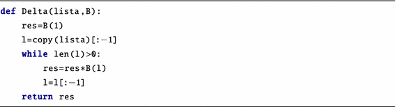
Delta
-
Input:
A list of consecutive numbers \([i,\dots ,j]\) and a braid group.
-
Output:
The half-twist braid involving the strands \(i,\dots ,j\).
-
Input:
-
(S2)
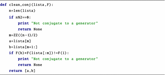
clean_conj
-
Input:
A list of numbers \([i,\dots ,j]\) and a free group. The list of numbers represents the Tietze representation of an element x in the free group (with generators \(g_j\)).
-
Output:
It returns None if x is not conjugate to a generator. If it is, it returns a list \([[i],[j_1,\dots ,j_r]]\) such that \(x=x_i^{x_{j_1}\cdot \ldots \cdot x_{j_r}}\).
-
Input:
-
(S3)
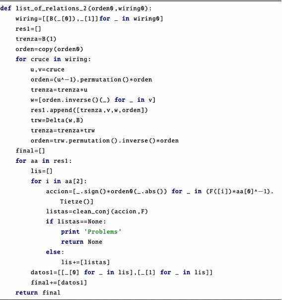
list_of_relations_2
-
Input:
A permutation to indicate the order of the lines in the beginning and a wiring diagram, see “Coding the wiring diagrams ” in Appendix. For each crossing we give a list with two members: the braid from the previous crossing, and the lines in the crossing. We assume a generic wiring diagram.
-
Output:
It returns the presentation of the group, as a list of elements with two entries; the first one is a list \([i_1,\dots ,i_r]\), \(r\ge 2\); the second one is a list of r lists, which represent the Tietze representation of words \(w_1,\dots ,w_r\). This element means that \(x_{i_1}^{w_1}\cdot \ldots \cdot x_{i_r}^{w_r}\) commutes with \(x_{i_1}^{w_1},\ldots , x_{i_r}^{w_r}\) (note that in other papers the reversed product is used).
-
Input:
-
(S4)
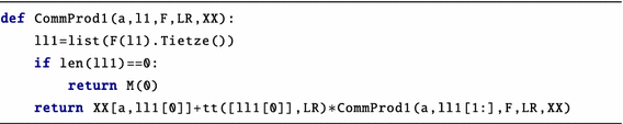
CommProd1
-
Input:
A number \(a\in \{1,\dots ,n\}\), a list representing a element x in the free group, the free group \(\mathbb {F}_n\) and the ring of Laurent polynomials in n variables and a dictionnary X associating to each [i, j] an element in the free module over the Laurent ring polynomial.
-
Output:
The element \([g_a,x]\) written as an element of the Alexander invariant M.
-
Input:
-
(S5)
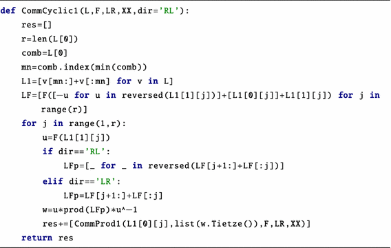
CommCyclic1
-
Input:
A list L, like the output of list_of_relations_2, the free group \(\mathbb {F}_n\) and the ring of Laurent polynomials in n variables, a dictionnary X associating to each [i, j] an element in the free module over the Laurent ring polynomial and a variable indicating the direction of the product yielding the local central element (set by default to RightLeft).
-
Output:
The list of elements in the Alexander invariant induced by the relations given by L.
-
Input:
-
(S6)
tt
-
Input:
A list of non-zero integers and a ring of Laurent polynomials in n variables.
-
Output:
The monomial defined by the list.

-
Input:
-
(S7)
MatTrunc
-
Input:
A matrix with coefficient in a power series ring.
-
Output:
The matrix where each entry has been truncated to level 2.
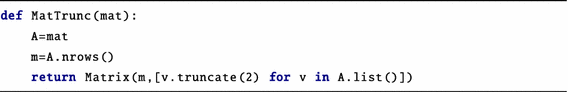
-
Input:
-
(S8)
EscalonarM2
-
Input:
A matrix over the power series ring representing a list of homogeneous linear equations with unknowns \(x_{i,j}\) and the number of lines n.
-
Output:
Let \(\mathcal {B}\) as in Step 1; each column of this matrix is the expression of the corresponding \(x_{i,j}\) in terms of the elements \(x_{k,l}\), \((k,l)\in \mathcal {B}\) in the Alexander invariant over the power series ring.
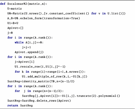
-
Input:
-
(S9)
ImagenMorfismo
-
Input:
A list [i, j] representing the commutator \(x_{i,j}\), a dictionnary XX associating to each [i, j] an element in the free module over the Laurent ring polynomial, a dictionnary YY associating to each [k, i, j] the unknown \(x_{k,i,j}\), representing \([x_k,[x_i,x_j]]\equiv (t_k-1)x_{i,j}\equiv s_kx_{i,j}\), S is a polynomial ring, LRv is the Laurent Ring with coefficients in the unknowns, dicv is the evaluation \(t_i\mapsto 1+s_i\) and inc is as in Step 1.
-
Output:
We consider the group of Step 5. This function uses it to express the image of \(x_{i,j}\).
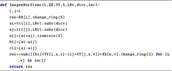
-
Input:


Rights and permissions
About this article

Cite this article
Artal Bartolo, E., Cogolludo-Agustín, J.I., Guerville-Ballé, B. et al. An arithmetic Zariski pair of line arrangements with non-isomorphic fundamental group. RACSAM 111, 377–402 (2017). https://doi.org/10.1007/s13398-016-0298-y
Received:
Accepted:
Published:
Issue Date:
DOI: https://doi.org/10.1007/s13398-016-0298-y