Joint delay and direction of arrivals estimation in mobile communications

Abstract

In this paper, we present a novel and precise way of estimating the direction and delay of arrivals in multipath environment for channel estimation purposes. Recently, super-resolution methods have been widely used for high-resolution direction of arrival (DOA) or time difference of arrival (TDOA) estimation. The proposed algorithm, called JDTDOA, is applicable to space–time channel estimation for space–time processing systems that employ hybrid DOA/TDOA technology. The estimator is based on conventional MUSIC algorithm to find the DOA and uses a standard correlator along with spline interpolation to find the TDOA of each arrival. In the interest of estimating the channel’s characteristics, each direction must be associated with its proper delay of arrival. To achieve this, we suggest a very simple and optimum beamforming by performing maximum variance distortionless response applied to each DOA found. The output at each DOA beamforming process gives the recovered signal from the relevant direction. A correlation is then made between each recovered signals which can be interpolated by cubic spline. The peak in correlation figure indicates the specific delay between the signal arrivals coming from the two considered direction.

1 Introduction

Nowadays, the increasing need in high-speed and high-quality wireless communications makes rigorous channel estimation critical in mobile terminals and networks. Improvements of the performance regarding bit error rate (BER) by more precise channel characteristics estimation is therefore an ongoing topic in mobile radio research and development as recent publications like [1, 2] and many more suggest.

In space–time processing systems, channel characteristics such as direction and time difference of arrival (DOA and TDOA respectively) are required to enhance the reception of the transmitted signal. That capability is especially beneficial in multipath environments, where multiple delayed and faded reflections are combined to one direct signal. By estimating direction and time delay of arrival, the received signals from different paths (direct signal and multiple reflected signals) can be weighted and shifted to get the stronger signal. This principle is used in many algorithms like the one proposed in [3] or the algorithm which we use in Rake receivers [4].

With this in mind, it is clear that the accuracy of DOA and TDOA measurements as well as a proper match between the delays and directions is important. It is therefore desirable to seek a procedure that automatically yields and sorts the delay-angle pairs in a straightforward and highly precise way.

For that matter, some algorithms were suggested such as the one proposed in [5]. However, those algorithms require a known sequence of symbols, a preamble, to retrieve the time delays between each arrival. Other joint DOA and TDOA estimation algorithms are proposed in [6] and [7]. Since their models for time delays are taken from the known modulation pulse shape of one symbol, those algorithms do not need any preamble. On the other hand, they are limited to delays smaller than the symbol duration. In mobile communication, time delays between different paths are most likely to be longer than the symbol rate. In [8] and [9], algorithms are proposed to estimate time delays and directions of arrivals without the use of any preamble. Nonetheless, those algorithms only work for ultra-wide band systems.

In this work, a practical method to estimate TDOA associated with DOA information in the presence of multipath without any preamble sequence is proposed. By using high resolution, we focus on estimating the DOA and TDOA of each narrowband arrival signal, which are two closely related aspects of array processing.

To do so, we propose to use the conventional MUSIC algorithm [10] and the Capon beamforming [11] in conjunction with the correlation function. The new proposed numerical method is able to associate correctly the DOA from the MUSIC algorithm and TDOA from the correlator. To our knowledge, no other existing algorithm is able to jointly estimate of TDOA/DOA without preamble, considering also intersymbol interference (ISI) within symbol and between symbols.

2 System model

The system model considered in this work consists of a linear uniform array antenna of $N$ identical elements, on which we have the impinging arrivals for one user. The $M$ signals consist of one direct signal and $M-1$ reflected ones. Since the MUSIC algorithm is used to estimate the direction of arrivals (DOAs), the number of wavefront arrivals, or signals, must be smaller than the number of elements in the array antenna, as suggested in [10].

Figure 1 illustrates the narrowband signal from one user considered as a source. Only the signal $s_m(t)$ from this user is shown. We can also extend the proposed algorithm to consider several users with different signals and more reflections. The analytic received signal is composed of the sum of $M$ source signals arriving from different angles and at different times. Each reflection signal is in fact a delayed and weighted copy of the direct signal. The signal received from the array is the $N\times 1$ complex vector ${\varvec{x}}(t)$. We can express the output vector ${\varvec{x}}(t)$ by defining at first ${s}_m(t)$ as

$$\begin{aligned} s_m(t)=\alpha _m s_d(t-T_m) \end{aligned}$$

(1)

where $\alpha _m$ and $T_m$ are the (arbitrary) amplitude and time delay of each signal path, respectively. In our assumption, $s_d(t)$ is the direct signal received at the first element with $\alpha _d=1$ and $T_d=0$; $d$ is the index of the direct signal.

Fig. 1

Uniform array antenna with two impinging signals

Then, we define ${\varvec{x}}(t)$ as the snapshot signal at the output of the $N$ antennas of the array at the time $t$ and express it as

$$\begin{aligned} {\varvec{x}}(t)=\sum _{m=1}^M {\varvec{s}}_m(t)+{\varvec{n}}(t) \end{aligned}$$

(2)

where

$$\begin{aligned} {\varvec{s}}_m(t)=\left[ \begin{array}{l} s_m (t) \\ s_m (t - \tau _m ) \\ \vdots \\ s_m (t - (N-1)\tau _m ) \\ \end{array} \right] . \end{aligned}$$

(3)

Since the delay of the wavefront arrival between the first element and the element $m, \tau _m$, is small with respect to the inverse of the signal bandwidth, we can replace this delay by a phase shift in an analytic signal representation. So we can rewrite (3) as

$$\begin{aligned} {\varvec{s}}_m(t)= \left[ \begin{array}{l} 1 \\ e^{ - j2\pi f_c \tau _m } \\ \vdots \\ e^{ - j2\pi f_c (N-1)\tau _m } \\ \end{array} \right] s_m (t). \end{aligned}$$

(4)

The vector in (4) is a $N \times 1$ vector which is known as direction vector or steering vector and expressed as

$$\begin{aligned} {\varvec{a}}(\theta _m )= \left[ 1,\,e^{ - j2\pi f_c \tau _m } ,\,\ldots , e^{ - j2\pi f_c (N-1)\tau _m} \right] ^\top . \end{aligned}$$

(5)

We can also define the phase shift of each narrowband arrival signal as:

$$\begin{aligned} \varphi _m=2 \pi f_c\tau _m=\frac{2\pi f_c D}{c}\, \sin (\theta _m). \end{aligned}$$

(6)

The symbol $\top$ denotes transpose, $f_c$ is the carrier frequency of the incident signals, and $\tau _m$ is the delay taken by the $m$-th signal path between two adjacent elements; $D$ is the interelement spacing and ${\varvec{n}}(t)$ is the $N\times 1$ complex additive noise vector. The noise at different elements of the array antenna can be considered as zero-mean Gaussian stationary random processes and independent from each element. So the noise at the antenna elements is mutually uncorrelated and also it is uncorrelated with the signals.

The delay from one component of the arrival signal impinging between adjacent elements of the array antenna ($\tau _m$) is caused by the path length difference $\Delta _m$ as seen in Fig. 1. This delay is comparable to the period of the carrier $f_c$, and much smaller than the duration of autocorrelation of emitted signal (or just the direct signal). So, it can be related to a phase shift. On the other hand, the delays ($T_m$) between the components are larger than the duration of autocorrelation of emitted signal. Therefore, these components are non correlated between themselves and we can consider them as independents sources. If correlation occurs, it is possible to use a spatial smoothing technique to make some decorrelation.

The $N\times N$ autocorrelation matrix of the array output vector ${\varvec{x}}(t)$, is expressed by ${\varvec{R}}_{xx}$ and written as

$$\begin{aligned} {\varvec{R}}_{xx}&= E\left\{ {\varvec{x}}(t){\varvec{x}}^H (t) \right\} \nonumber \\&= {\varvec{A}}{\varvec{R}}_{ss}{\varvec{ A}}^H + \sigma ^2 {\varvec{I}}_N \end{aligned}$$

(7)

where ${\varvec{A}}$ is the steering matrix:

$$\begin{aligned} {\varvec{A}}=\left[ {\varvec{a}}(\theta _1),\,{\varvec{a}}(\theta _2),\,\ldots ,\,{\varvec{a}}(\theta _M)\right] . \end{aligned}$$

(8)

The symbol $H$ denotes the Hermitian transpose. The variables $\sigma ^2$ and ${\varvec{I}}_N$ are the variance of the additive noise and identity matrix, respectively, because the noises are independent from one element to the others; ${\varvec{R}}_{ss}$ denotes the $M\times M$ autocorrelation matrix for source signals:

$$\begin{aligned} {\varvec{R}}_{ss}&= E\left\{ {\varvec{s}}(t){\varvec{s}}^H (t) \right\} = \text{ diag }\{\mu _1,\,\mu _2,\,\ldots ,\,\mu _M\} \end{aligned}$$

(9)

$$\begin{aligned} {\varvec{s}} (t)&= \left[ \begin{array}{l} s_1 (t) \\ s_2 (t) \\ \vdots \\ s_M (t) \\ \end{array} \right] . \end{aligned}$$

(10)

The matrix ${\varvec{R}}_{ss}$ is a diagonal matrix since the arrivals are considered as independent sources, as stated in [10]. The variable $\mu _m$ then corresponds to the power of the $m$-th arrivals.

3 Review of algorithms

The proposed algorithm is based on the fusion of MUSIC algorithm and beamforming. We will make a short review of these two.

3.1 MUSIC algorithm

The original or conventional MUSIC algorithm [10] was proposed to estimate the directions of arrival of the uncorrelated or partially correlated signals. Since this algorithm exceeds the Rayleigh resolution criterion, it is classified as high-resolution algorithm. There are $N-M$ eigenvectors associated with the kernel (null space) of the ${\varvec{R}}_{xx}$ in a case without noise. That is valid only when source signals are independent or not completely correlated. To be sure that we have independent $s_m(t)$, the delay $T_m$ should be greater than the autocorrelation of $s_d(t)$. The matrix ${\varvec{V}}_n$ is made from the eigenvectors ${\varvec{v}}_i$ associated with the $N-M$ smaller eigenvalues of ${\varvec{R}}_{xx}$ as

$$\begin{aligned} {\varvec{V}}_n=\left[ {\varvec{v}}_{M+1},\,{\varvec{v}}_{M+2},\,\ldots ,\,{\varvec{v}}_{N}\right] . \end{aligned}$$

(11)

Due to ${\varvec{R}}_{xx}$ matrix properties, all steering vectors, ${\varvec{a}}(\theta _m)$ are orthogonal to all vectors in ${\varvec{V}}_n$. Conventional MUSIC is based on this fact and we can write:

$$\begin{aligned} {\varvec{a}}^H (\theta _m ){\varvec{V}}_n {\varvec{V}}_n^H {\varvec{a}}(\theta _m ) = 0 \quad (m = 1,2,\ldots ,M) \end{aligned}$$

(12)

where index $m$ indicate the signal index ($m=d$ for direct signal, $m=1\ldots M\ne d$ for reflected ones).

Therefore, by exploiting the orthogonality between the steering vector and the null space in (12), we can express the MUSIC spectrum for spatial estimation as

$$\begin{aligned} P(\theta ) = \frac{1}{{\varvec{a}}^H (\theta ){\varvec{V}}_n {\varvec{V}}_n^H {\varvec{a}}(\theta )} \end{aligned}$$

(13)

where ${\varvec{a}}^H (\theta )$ is constructed as in (5) with different values of $\theta$. Peaks of the MUSIC spectrum correspond to the direction of arrival of the signals impinging on the array antenna.

3.2 MVDR beamforming

Performing optimum beamforming maximum variance distortion response (MVDR) [11] (also called Capon beamforming) for array antenna involves maximization of the signal-to-interference ratio (SIR) in a given direction. The signals coming from other directions are then considered as interference.

We have to estimate the complex $N\times 1$ weight vector ${\varvec{w}}$, for conventional Capon Beamforming by maximizing the SIR. The input vector is written as

$$\begin{aligned} {\varvec{x}}=\alpha _{\theta }{\varvec{a}}(\theta )+{\varvec{b}}_{\theta } \end{aligned}$$

(14)

where $\alpha _{\theta }$ is the amplitude of the signal coming from direction $\theta$ (if no signal is coming from this direction, then $\alpha _\theta =0$), ${\varvec{b}}_{\theta }$ is the sum of all vector components not colinear with ${\varvec{a}}(\theta )$, i.e., all signals coming from others directions than $\theta$. The SIR is now expressed by:

$$\begin{aligned} \text{ SIR } = \frac{\left| \alpha _\theta {\varvec{w}}^H (\theta ){\varvec{a}}(\theta ) \right| ^2 }{ {\varvec{a}}^H (\theta ){\varvec{R}}_{bb} {\varvec{a}}(\theta )} \end{aligned}$$

(15)

where:

$$\begin{aligned} {\varvec{R}}_{bb}= {\varvec{R}}_{xx} - \mu _\theta {\varvec{a}}(\theta ){\varvec{a}}^H (\theta ) \end{aligned}$$

(16)

and

$$\begin{aligned} \mu _\theta = \text{ var }\{ \alpha _\theta \}. \end{aligned}$$

(17)

Applying the Schwarz inequality to (15) yields:

$$\begin{aligned} \text{ SIR } \le \left| {\alpha _\theta } \right| ^2 {\varvec{a}}^H (\theta ){\varvec{R}}_{bb} ^{-1} {\varvec{a}}(\theta ). \end{aligned}$$

(18)

The maximum of this ratio is obtained for:

$$\begin{aligned} {\varvec{w}}_{\theta }=\beta {\varvec{R}}_{bb} ^{-1} {\varvec{a}}(\theta ) \end{aligned}$$

(19)

where $\beta$ is a proportionality constant. By using the matrix inversion lemma and Eq. (16), we can write:

$$\begin{aligned} {\varvec{R}}_{bb} ^{-1} = {\varvec{R}}_{xx} ^{-1} + \mu _\theta \frac{{\varvec{R}}_{xx} {\varvec{a}}(\theta ){\varvec{a}}^H (\theta ){\varvec{R}}_{xx} ^{-1}}{1 - \mu _\theta {\varvec{a}}^H (\theta ){\varvec{R}}_{bb} ^{-1} {\varvec{a}}(\theta )}. \end{aligned}$$

(20)

Applying (20) in (19), we retrieve the well-known expression of the MVDR beamforming as

$$\begin{aligned} {\varvec{w}}_\theta = \frac{{\varvec{R}}_{xx}^{-1} {\varvec{a}}(\theta )}{{\varvec{a}}^H (\theta ){\varvec{R}}_{xx}^{-1} {\varvec{a}}(\theta )} \end{aligned}$$

(21)

4 Proposed algorithm

Determining the time delays of the arrival signals in a multipath environment without knowledge about the emitter signal is one objective of this paper. To estimate adequately the propagation channel, we must find the delays of different impinging signals in each element of antenna. To do this, we can use correlation function as it is done in numerous papers. In most proposed algorithms, the delay can be found using correlation function of the received signal and the transmitted one. The disadvantage of the conventional approach is that a known transmitted signal to which the received signal can be correlated is needed. Another problem is that these delays cannot be associated with their respective DOA. In other words, by using directly the correlation function, we can find different peaks which are related to the delays of arrival, but we can not associate each delay with its proper DOA.

Two main ways can be taken. It is possible to deal with these problems by obtaining jointly the direction and the delay by a two parameters directional vector to create ${\varvec{a}}(\theta ,t)$. However, even 2D MUSIC algorithm [12] cannot be used without any knowledge of the signal in time to create a model. Also, 2D MUSIC requires a search in a two-dimensional space of the pseudospectrum $P(\theta ,t)$ as described in (13). A peak must appear at each $(\theta _m,T_m)$ so the association between direction and delay is made directly. The complexity of the search is problematic: scanning the entire space can take a very long time. We recall that 2D MUSIC always requires a preamble to treat ISI between symbols, or a pulse shape model for ISI within symbol only.

The other possible process is to consider the direction and delay separately by applying a conventional cross-correlator between the signal at one receiving element and a copy of the direct signal to estimate all delays of arrival signals. The MUSIC algorithm can also be applied to estimate all directions of arrival. Two limitations appear with this approach. Firstly, it is still necessary to include a preamble signal to create the copy of the direct signal alone. Without an idea of the direct signal, the autocorrelation can be used instead but many peaks will appear at all positions $T_p-T_q$ ($p\ne q$) and not just at positions $T_m-T_d$ (where the index $m=d$ corresponds to the direct signal). Secondly, the delays and directions are estimated separately. Another step is needed to match or associate each estimated delay with one direction among those estimated.

So, we propose to proceed in an intermediate way. Rather than making completely independent searches of directions and delays, we suggest to perform the second search (in $t$) considering the result of the first search (in $\theta$). The proposed algorithm has many advantages: No known signal is needed anymore; and in addition, not only the association is made directly, but also the two searches are performed in a simple way.

The steps are as follows:

• (a) MUSIC algorithm shown in Sect. 3.1 is applied to find all directions of arrival $\theta _m$. The $\theta _m$ are the $M$ maximas of the function $P(\theta )$ of Eq. (13). We can also use Root-MUSIC [13] to estimate directly all directions of arrival without plotting the pseudospectrum.

• (b) A new signal is generated at the output of the array antenna by applying a beamforming in one of the directions determined in the previous step. This beamformer tries to eliminate all arrival signals except one having the index $m$ in the direction $\theta _m$. The simple beam steering can be made by phasing the array to steer the main lobe in the direction $\theta _m$. This step, which is fairly simple, is the main contribution of this paper. The idea is important because at the end of this step, we now have a pseudocopy of $s_m(t)$, named $y_m(t)$, defined in (1) by summing the signals from all elements as in a phased array antenna:

  $$\begin{aligned} y_m(t) = {\varvec{w}}^H(\theta _m) {\varvec{x}}(t)\approx \beta s_m(t). \end{aligned}$$

  (22)

  For the case of simple beam steering on a linear uniform array, we have ${\varvec{w}}={\varvec{w}}_a$ so that:

  $$\begin{aligned} {\varvec{w}}_a(\theta _m) \,=\, [1,\,e^{-j\varphi _m},\,e^{-j2\varphi _m},\,\ldots ,\,e^{-j(N-1)\varphi _m}]^\top \qquad \end{aligned}$$

  (23)

  where $\beta$ in a proportionality constant, $\varphi _m$ is calculated as in Eq. (6), ${\varvec{x}}(t)$ is the snapshot vector defined in (2). The simple beamsteering works well to retrieve the pseudocopies $y_m(t)$ but the signals coming from directions close to $\theta _m$ are just slightly attenuated, not enough for impressive results. That is why we suggest using the MVDR beamforming shown in Sect. 3.2 instead. With MVDR, ${\varvec{w}}={\varvec{w}}_b$ is calculated as in (21):

  $$\begin{aligned} {\varvec{w}}_b(\theta _m) \,=\, \frac{{\varvec{R}}_{xx}^{-1}{\varvec{a}}(\theta _m)}{{\varvec{a}}^H(\theta _m){\varvec{R}}_{xx}^{-1}{\varvec{a}}(\theta _m)} \end{aligned}$$

  (24)

  which gives an $y_m(t)$ much more closely proportional to $s_m(t)$ since all contributions from others directions than $\theta _m$ are completely removed.

• (c) A conventional cross-correlation is now made between $y_m(t)$ from $m=1\ldots M$ (which contains in theory only the signal of the $m$-th arrival) and any other arrival signal among the $(M-1)$ ones, called $y_p(t)$ (the $p$-th arrival), where $p$ can be taken in $1\ldots M$. That gives the output $u_{m_p}$ such that:

  $$\begin{aligned} u_{m_p}(\tau ) \,=\, y_m(t)\circ y_p(t) \end{aligned}$$

  (25)

  where $\circ$ is the correlation function. Since time $t$ is discrete, we can add spline or even linear interpolation on $y_m(t)$ and $y_p(t)$ in order to perform correlation for $\tau$ within a fraction of the sampling time $T_s$ ($\tau = k \times T_s/q$ where $k$ and $q$, the interpolation factor, are integers). We could therefore achieve better time delay estimations than with $\tau$ as a multiple of $T_s$ ($\tau = k \times T_s$). The correlation function is maximum when $\tau$ corresponds as closely as possible to the delay between $y_m$(t) and $y_p(t)$. Since $y_m(t)$ is the pseudocopy of $s_m(t), y_m(t)$ is proportional to $s_d(t-T_m)$ according to Eq. (1). The same reasoning is applied to $y_p(t)$ with $s_d(t-T_p)$. Then the peak of $u_{m_p}(\tau )$ gives the delay difference between the $m$-th and the $p$-th arrivals:

  $$\begin{aligned} T_m-T_p=T_{m,p} = \arg \mathop {\max }\limits _\tau \left( u_{m_p} (\tau )\right) . \end{aligned}$$

  (26)

  After obtaining all $T_m-T_p$ for $m=1\ldots M$ for a given $p$, we can find the index $d$ of the direct signal. In fact, the value of $m$ giving the most negative $T_{m,p}$ (which may be 0, if we select by chance $p=d$) corresponds to the index $d$ of the direct signal since the direct signal is always the first arrival. Thus, we have:

  $$\begin{aligned} d=\arg \min _{m} \left( T_m-T_p\right) . \end{aligned}$$

  (27)

  Consequently, the delay for each arrival compared to the direct signal can be obtained as

  $$\begin{aligned} T_m&= \left( T_m-T_p\right) -\left( T_d-T_p\right) \nonumber \\&= \arg \max _{\tau } \left( u_{m_p}(\tau )\right) - \arg \max _{\tau } \left( u_{d_p }(\tau )\right) \end{aligned}$$

  (28)

  since $T_d$ is assumed to be 0.

To associate each DOA with the correct TDOA, the algorithm considers one DOA at a time from those provided by the MUSIC spectrum and calculates the beamformer output signal $y_m(t)$ from each of them. The advance ($T_{m,p}<0$ ) or the delay ($T_{m,p}>0$) of the $m$-th arrival compared to a given $p$-th arrival in (26) is extracted by the peak location in $\tau$ of the correlation function (25).

5 Numerical examples

The modulation used in the subsequent examples is QPSK at the symbol rate of 1 MHz with one sample per symbol (sampling rate of 1 MHz); however, it can be easily replaced by any other kind of modulation.

The array is made with $N=8$ elements having an interelement spacing of $d=\lambda /2$. An estimation of the covariance matrix is computed from $K=500$ snapshots so that ${\varvec{R}}_{xx}\approx \frac{1}{K}\sum _k {\varvec{x}}(t=kT_s){\varvec{x}}(t=kT_s)^H$. A snapshot is taken at an interval corresponding to the symbol duration $T_s=1.0\,\upmu$s. When cross-correlation is made between signals, the resolution is then $1\,\upmu$s. Those parameters are used in the two following numerical examples.

• (a) To show that the algorithm is able to associate adequately direction and delay of arrivals, we consider direct signal coming from the source at $\theta _2=30^\circ$ with a signal-to-noise ratio $\text{ SNR }_m=\frac{\mu _m}{\sigma ^2}$ of $\text{ SNR }_2=14$ dB. The index for the direct signal is then $d=2$ ($T_2=0$). Three reflected signals are impinging on the array from $\theta _1=-10^\circ , \theta _3=40^\circ$ and $\theta _4=70^\circ$ with delay from the direct signal equal to $T_1=11.5, T_3=2.8$ and $T_4=18.4\,\upmu$s and $\text{ SNR }_1=20, \text{ SNR }_3=6$ and $\text{ SNR }_4=17$ dB. So, we have $M=4$ and:

  $$\begin{aligned} \varvec{\theta }&= [-10^\circ ,\,30^\circ ,\,40^\circ ,\,70^\circ ] \\ {\varvec{T}}&= [11.5,\,0,\,2.8,\,18.4]\,\upmu \hbox {s}. \end{aligned}$$

  The MUSIC algorithm using Eq. (13) is now applied and the pseudospectrum is plotted in Fig. 2. From this figure, the $M=4$ peaks give the directions of arrival. We found, for this example, an estimated vector of DOAs

  $$\begin{aligned} \hat{\varvec{\theta }}=[-9.92^\circ ,\,30.12^\circ ,\,39.86^\circ ,\,70.18^\circ ]. \end{aligned}$$

  However, at this step, we are not able to determine which one of the $M$ direct and reflected paths corresponds to each of those angles. If we apply autocorrelation directly on $x_n(t)$ (we recall that $x_n(t)$ is the signal received at the $n$-th element), we obtain a lot of peaks (more than 4) at all positions $T_p-T_q$, where $1\le p, q\le M$. Applying rather cross-correlation between $x_n(t)$ and $s_d(t)$ ($s_d(t)$ with $d=2$ is the direct signal alone), we obtain four peaks at positions $T_{m^\prime }-T_d$ in a different order $m^\prime$ as seen on Fig. 3. Consequently, the four peaks are badly indexed but closely estimated at $\breve{{\varvec{T}}}\approx [0,\,2,\,11,\,18]\,\upmu$s; vector $\breve{{\varvec{T}}}$ contains an estimation of TDOAs in increasing order which is not the right order considering the signal order in the vector of estimated directions of arrival $\hat{\varvec{\theta }}$. We recall that the exact TDOA vector is ${\varvec{T}}=[11.5,\,0,\,2.8,\,18.4]\,\upmu$s. The problem now is to associate each TDOA to each DOA obtained in the previous step. Moreover, we need to know the content of the emitted signal (or at least just have the direct signal) when proceeding in this manner. That is why step (b) in the proposed algorithm is so important. For each $\theta$ in vector $\hat{\varvec{\theta }}$, we must obtain the pseudocopy $y_m(t)$. Beginning with $\theta =-9.92^\circ$ ($m=1$, the order is not important), we compute the corresponding weight vector ${\varvec{w}}_a$ or preferably ${\varvec{w}}_b$ following (23) or (24) taking $\theta _m=-9.92^\circ$ (the weight vector ${\varvec{w}}_a$ gives inferior performances, but it is easier and faster to obtain since it does not require the covariance matrix inversion). We retrieve $y_1(t)$ by applying the weight vector ${\varvec{w}}_b$ instead to the received signal as in (22). The signal $y_1(t)$ should be close to $s_1(t)=\alpha _1s_d(t-T_1)$. And so on for $\theta =30.12^\circ ,\, 39.86^\circ$ and $70.18^\circ$ in this example. Figure 4 shows the $M=4$ cross-correlations between $y_1(t)$ and $y_m(t)$ giving the functions $u_{m_1}(\tau )$ ($p=1$) according to (25). From these curves, we see that $d=2$, since the peak appears at the $-11\,\upmu$s (we recall that the resolution of cross-correlation is $T_s=1\,\upmu$s) in the upper-right graph $m=2$, which is the most negative peak location in $\tau$ for the 4 correlation functions. We can also observe that the DOA corresponding to $\theta =-9.92^\circ$ has index $m=1$ since the peak is at $\tau =0$ as for the autocorrelation function. Then the arrival coming from $\theta _1=-9.92^\circ$ is $11\,\upmu$s behind the arrival coming from $\theta _2=30.12^\circ$. The peak of the correlation function $u_{3_1}(\tau )$ ($\theta _3=39.86^\circ$) is approximately at $\tau =-9\,\upmu$s then the arrival coming from $\theta _1=-9.92^\circ$ is $9\,\upmu$s behind the arrival coming from $\theta _3=39.86^\circ$. From correlation function $u_{4_1}(\tau )$, the arrival coming from $\theta _4=70.18^\circ$ is in advance by close to $7\,\upmu$s from the arrival coming from $\theta _1=-9.92^\circ$. The estimated time delays from these graphs (with $p=1$) following (28) are now in the right order:

  $$\begin{aligned} \hat{{\varvec{T}}}_1&= ([0,\,-11,\,-9,\,7]-[-11,\,-11,\,-11,\,-11])\,\upmu \hbox {s}\\&= [11,\,0,\,2,\,18]\,\upmu \hbox {s}. \end{aligned}$$

  In our simulation, we made the first reflection (arrival #3) very weak and very near in time (just $2.8\,\upmu$s late) compared to the direct signal (#2). So, the signal from this reflection is drowned out by the direct signal. We observe on Fig. 3 small peaks at the right of the first peak for all correlation curves. However, the proposed algorithm performs very well to extract the delay $T_3$ even if this weak signal is very close to the strongest one. That explains why the algorithm succeeds in associating the delays and directions. Figure 5 shows the results when we repeat the same process but taking DOA at $39.86^\circ$ (arrival #3), the corresponding weight vector ${\varvec{w}}_b$, to compute $y(t)$ from which are found the 4 cross-correlation functions $u_{m_p}(\tau )$. Again, from graph at lower-left, we see that $p=3$ since the peak is at $\tau =0$ in this graph. The figure indicates that

  $$\begin{aligned} \hat{{\varvec{T}}}_3&= ([9,\,-3,0,\,16]-[-3,\,-3,\,-3,\,-3])\,\upmu \hbox {s}\\&= [12,\,0,\,3,\,19]\,\upmu \hbox {s}. \end{aligned}$$

  This new vector of estimated delays of arrival obtained with $p=3$ is slightly different from this with $p=1$, but it is still in right order. If we repeat the process with $p=2$ and $p=4$, we find 2 others vectors of estimated delays $\hat{{\varvec{T}}}_2$ and $\hat{{\varvec{T}}}_4$. The means of these $M=4$ vectors gives:

  $$\begin{aligned} \bar{\hat{{\varvec{T}}}} \,=\, \frac{1}{4}\sum _{p=1}^4 \hat{{\varvec{T}}}_p \,=\, [11.25,\,0,\,2.5,\,18.75]\,\upmu \hbox {s} \end{aligned}$$

  which is very close to the vector of exact delays. If a cubic spline interpolation is applied before the cross-correlation (with an interpolation period of $T_s/10$, therefore $q = 10$), we can retrieve even more closely the time delays:

  $$\begin{aligned} \bar{\hat{{\varvec{T}}}}_{spline} \,=\, [11.43,\,0,\,2.75,\,18.32]\,\upmu \hbox {s}. \end{aligned}$$

  Fig. 2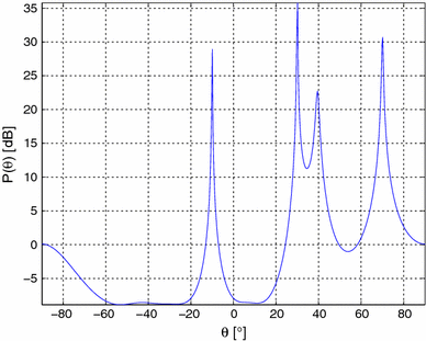

  

  MUSIC pseudospectrum from simulation of the numerical example

  Fig. 3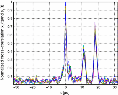

  

  Correlation function curves between $x_n(t)$ ($n=1,2,\ldots 8$) and the direct signal $s_d(t)$ (used to find the delays)

  Fig. 4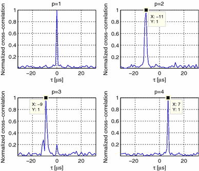

  

  Correlation functions curves $u_{m_1}(\tau )$ for each value of $m$ from 1 to $M=4$ (taking $\theta _1=-9.92^\circ$, $\theta _2=30.12^\circ$, $\theta _3=39.86^\circ$ and $\theta _4=70.18^\circ$) (used to find the associated delay)

  Fig. 5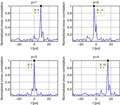

  

  Correlation function curves $u_{m_3}(\tau )$ for each value of $m$ from 1 to $M=4$ ($\theta _1=-9.92^\circ$, $\theta _2=30.12^\circ$, $\theta _3=39.86^\circ$ and $\theta _4=70.18^\circ$) (used to find the associated delay)

• (b) In order to show the accuracy and precision of the JDTDOA algorithm, we consider two signal arrivals: a direct signal at $\theta _2 = 30^\circ$ and $T_2 = 0\,\upmu$s and its reflection at $\theta _1 = -10^\circ$ and $T_1 = 11.6\,\upmu$s (unless otherwise specified). The two signals have the same SNR, which is described along Figs. 6, 7 and 8. Since the MUSIC algorithm’s performance is already studied in [14, 15] and [16], this example focuses more specifically on time delay estimation. The MVDR beamforming is applied on the observed signals to create the two pseudocopies of the direct signal $s_2(t)$ and the reflected one $s_1(t)$. This beamforming is done using the estimated DOAs and using the exact DOAs. The correlation function is then performed on the pseudocopies ($y_1(t)$ and $y_2(t)$) which are interpolated with cubic spline at each $T_s/10$ s. To obtain Fig. 6, those steps were repeated for different SNR. As seen in this figure, the root-mean-squared (RMS) error on the time delays with estimated DOA remains very low until a SNR of $-$5 dB. Under $-$5 dB, JDTDOA reach a limit where time delays cannot be estimated accurately. This limit is lower for time delays estimated with exact DOA. In Fig. 7, error is added on the estimated $\theta _1$ and the resulting inaccurate DOA is used in the MVDR beamforming. This figure shows that an error as great as $7.5^\circ$ is acceptable on $\theta _1$ in order to properly estimate and associate both delays. For Fig. 8, the MVDR beamforming is performed using the exact DOA and the correlation function estimate the delays for different time delays $T_1$. This figure illustrates the precision reached by the correlation with cubic spline interpolation. For ISI between symbols, the correlation (with cubic spline interpolation of $T_s/10$) can estimate each TDOA within a $T_s/10$ error. Nonetheless, for ISI within symbols, the delays cannot be estimated with high accuracy: For delays lower than $T_s$, the time delay $T_1$ is estimated to the nearest value (either 0 or $T_s$) leading to a higher RMS error. Also, it is expected that the RMS error on the time delay is lower for delays that are multiples of the sampling period $T_s$, since the correlation is then maximal on non-interpolated samples. Likewise, the RMS error is inferior for uneven multiples of $T_s/2$ because the correlation is then maximal halfway between non-interpolated samples. However, since the cubic spline interpolation does not follow the pulse shape model, other time delays lead to greater RMS error (near $T_s/10$).

  Fig. 6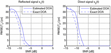

  

  Root-mean-squared error on the time delays $T_1$ and $T_2$ estimation in function of SNR. The time delays are estimated with pseudocopies formed by MVDR beamforming on the exact DOA and on the estimated DOA using MUSIC. Each RMSE value is calculated for 1,000 Monte Carlo simulations

  Fig. 7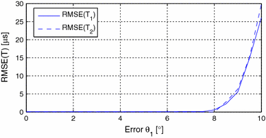

  

  Root-mean-squared error on the time delays $T_1$ and $T_2$ estimation for SNR of 5 dB in function of error on $\theta _1$. The time delays are estimated with pseudocopies formed by MVDR beamforming on the estimated DOA with the added error. Each RMSE value is calculated for 1,000 Monte Carlo simulations

  Fig. 8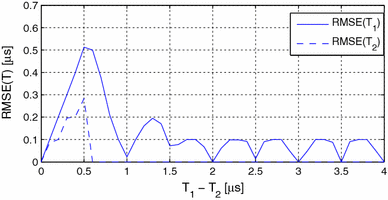

  

  Root-mean-squared error on the time delays $T_1$ and $T_2$ estimation for SNR of 5 dB in function of delay $T_1$ ($T_2$ always kept equal to 0 since $d=2$). The time delays are estimated with pseudocopies formed by MVDR beamforming on the exact DOA. Each RMSE value is calculated for 1,000 Monte Carlo simulations

6 Computational complexity

The 2D MUSIC [12] algorithm is selected as basis to compare the computational complexity even with the preamble requirement. The 2D MUSIC is able to find with high resolution and to associate appropriately DOA and TDOA of direct and reflected signals in multipath environment. The complexity is evaluated in terms of complex multiplications. Either 2D MUSIC or JDTDOA, the first steps are then same: form the covariance matrix ${\varvec{R}}_{{\varvec{xx}}}$ from the $K$ snapshots and make the eigen-decomposition of ${\varvec{R}}_{{\varvec{xx}}}$. The principle of 2D MUSIC is to search in a 2D plane using $\theta$ and $\tau$ as two distinct scanning parameters. As MUSIC, the steering vector ${\varvec{a}}(\theta , \tau )$ is projected in the noise subspace as in (13) whose eigenvector matrix ${\varvec{V}}_{\varvec{n}}$ form the basis. Each projection needs $(N\times (N-M) + (N-M))$ multiplications and one division (or one multiplication by the inverse). The pseudospectrum is then plotted in 3D for a grid having $n_\theta$ points in $\theta$ and $n_\tau$ points in $\tau$. Therefore, a total of $(N \times (N - M) + N - M + 1) \times n_\theta \times n_\tau$ multiplications is required for all combination of $\theta$ and $\tau$, besides the eigen-decomposition. After that, a procedure must be added to localize the $M$ peaks of the 2D pseudospectrum. Root-MUSIC could have been more interesting to reduce calculations and to avoid peaks retrieving in the pseudospectrum. Unfortunately, a version of Root-MUSIC having two scanning parameters does not exist until now. On the other hand, the proposed algorithm JDTDOA takes the following steps:

• The DOAs are found from 1D MUSIC requiring $(N \times (N - M) + N - M + 1) \times n_\theta$ multiplications. A procedure must be added to localize the $M$ peaks but in a 1D pseudospectrum which is simpler than 2D search. At this step however, the proposed algorithm can profit of Root-MUSIC to calculate the DOAs without peaks search and with a less computational complexity than 1D standard MUSIC pseudospectrum alone.

• To retrieve the ${\varvec{R}}_{{\varvec{xx}}}^{-1}$, we can use eigen-decomposition found previously. Moreover, ${\varvec{R}}_{{\varvec{xx}}}^{-1}$ can be approximated by a Moore–Penrose pseudoinverse using only the $M$ greater eigenvalues and the $M$ eigenvectors associated with those eigenvalues. After inverting all $M$ eigenvalues ($1/\lambda _m$), we need to achieve multiplications by the eigenvectors matrix on each side: ${\varvec{R}}_{{\varvec{xx}}}^{-1} = {\varvec{V}}_{\varvec{s}} \varvec{\Lambda }_{\varvec{s}}^{-1} {\varvec{V}}_{\varvec{s}}^H$ where ${\varvec{V}}_{\varvec{s}}$ corresponds to the $M$ eigenvectors and $\varvec{\Lambda }_{\varvec{s}}^{-1} = \text{ diag }\{ 1/\lambda _1, 1/\lambda _2,\ldots , 1/\lambda _M\}$. Therefore, $N \times M \times (N+1)$ multiplications must be done to retrieve ${\varvec{R}}_{{\varvec{xx}}}^{-1}$.

• For the next step, the weight vector ${\varvec{w}}_b(\theta _m)$ of MVDR is calculated as in (21). As part of the denominator and the numerator, ${\varvec{R}}_{{\varvec{xx}}^{-1}}{\varvec{a}}(\theta _m)$ can be computed once: $N\times N$ multiplications are needed for this operation. Then, $N$ multiplications are still needed for the denominator, and lastly, $N$ divisions are required. The weight vector is calculated for each $M$ directions. So, MVDR requires a total of $M \times (N^2 + 2N)$ multiplications.

• In this step, the pseudocopy of $s_m(t)$, corresponding to $y_m(t)$ is obtained from (22). The weight vector ${\varvec{w}}_b(\theta _m)$ is multiplied by the received signal vector $x(t)$ for each value of $t$ and for each $\theta = \theta _m$. This step takes a total of $K \times M \times N$ multiplications.

• Finally, the correlation (without interpolation) must be made $M$ times (for each source) following (25); each one needs $n_\tau$ multiplications for a total of $M \times n_\tau$.

Consequently, the JDTDOA takes $N^2 \times (n_\theta +2M)+N \times (n_\theta \times (1-M)+M \times (K+3))+n_\theta \times (1-M)+M \times n_\tau$ multiplications. Considering a system with $M = 4$ sources (one direct signal and three reflected ones) where the received signal on the $N = 8$ elements of an antenna array is sampled $K = 500$ times, as in our example. Considering also a realistic pseudospectrum where $n_\tau = 50$ (maximum delay of 25 symbols; a longer delay in unnecessary since the reflection arriving far away from the direct signal is insignificant in practice), $n_\theta = 180$ (a resolution of 1$^{\circ }$ is typical to separate each component of the received signal). In this condition, the 2D MUSIC algorithm needs up to 333,000 multiplications whether JDTDOA requires only 23,532 multiplications. Also, for 2D MUSIC, the extraction of peaks from the 2D pseudospectrum must be made to retrieve the direction and time delay of arrivals. For a human with his eyes and his brain, this process is easy, but it is very complex for a computer machine when some peaks are very smooth (not sharp). For JDTDOA, the DOAs can be extracted easily using Root-MUSIC at the first step of JDTDOA and the unique peak of the cross-correlation functions $u_{m_p}(\tau )$ is found taking $\tau$ giving the maximum value. Consequently, as mentioned in [17], the 2D MUSIC needs more calculus in spit of the good results achieved; these latter are however comparable to the ones from JDTDOA.

7 Conclusion

We have proposed a simple and precise method to estimate channel characteristics. The proposed method called JDTDOA is able to associate the directions and the delays of any arriving signal on an array antenna in a multipath environment, without any knowledge of an emitted data sequence (preamble). JDTDOA is based on a mixture of MUSIC estimation and MVDR beamforming. In fact, MUSIC is a high- resolution estimator for DOAs, while MVDR is optimal in the sense of SIR to eliminate undesired signal coming from others directions. The delays are extracted by using a simple correlator between the recovered copy of the different signals $y_m(t)$ with a reference one ($y_p(t)$).

The complexity of the JDTDOA is less than that 2D MUSIC algorithm working jointly in space and time to find the directions and the delays of arrival signals and this latter needs a preamble. Until today, JDTDOA is the only algorithm that can be applied to narrow band mobile communications while retrieving jointly DOA and TDOA without the use of any preamble for delay greater than one symbol (ISI between symbols). Although some algorithms use the pulse shape model instead of preamble, those are only able to consider ISI within symbol.

The resolution in direction depends on MUSIC estimation, which is known as a high-resolution algorithm. However, the resolution in delay is given by standard cross-correlations only. The resolution achieved in delay is, however, sufficient since it is less than a fraction of the sampling period. Because no second-order statistics are involved, high resolution is not reached. To increase this resolution, cubic spline interpolation can be used on the retrieved signals before the correlation. Again, we can use the means of TDOAs found using each of the $M$ recovered copies as the reference, one at a time. It is also possible to take more samples per symbol (oversampling), decreasing $T_s$. Another possibility is to adapt the algorithm in [18] for the cross-correlation profile.

References

Suryani, T., Hendrantoro, G.: Improvement in channel estimation and error rate performance in mobile cooperative ofdm systems with intercarrier interference. Int. J. Distrib. Sens. Netw. 2014 (2014). doi:10.1155/2014/509896
Yang, J., Lin, K., Zhao, X.: An improved channel estimation method based on jointly preprocessing of time-frequency domain in td-lte system. J. Netw. 9(4), 1047–1054 (2014)
Hew, N., Zein, N.: Space-time estimation techniques for utra system. In: First International Conference on 3G Mobile Communication Technologies, ser., no. 471. IET, pp. 281–287 (2000)
Chen, Y.F., Zoltowski, M.D.: Joint angle and delay estimation for ds-cdma with application to reduced dimension space-time rake receivers. In: Acoustics, Speech, and Signal Process, ser. ICASSP, vol. 5, pp. 2933–2936. IEEE (1999)
Singh, P., Sircar, P.: Time delays and angles of arrival estimation using known signals. Signal Image Video Process. 6(2), 171–178 (2012)
Wang, Y.-Y., Chen, J.-T., Fang, W.-H.: Tst-music for joint doa-delay estimation. IEEE Trans. Signal Process. 49(4), 721–729 (2001)
Zhang, X., Feng, G., Xu, D.: Blind direction of angle and time delay estimation algorithm for uniform linear array employing multi-invariance music. Prog. Electromagn. Res. Lett. 13, 11–20 (2010)
Navarro, M., Najar, M.: Frequency domain joint toa and doa estimation in ir-uwb. IEEE Trans. Wirel. Commun. 10(10), 1–11 (2011)
Lagunas, E., Nájar, M., Navarro, M.: Joint toa and doa estimation compliant with ieee 802.15. 4a standard. In: 2010 5th IEEE International Symposium on Wireless Pervasive Computing (ISWPC), pp. 157–162. IEEE (2010)
Schmidt, R.O.: Multiple emitter location and signal parameter estimation. IEEE Trans. Antennas Propag. 34(3), 276–280 (1986)
Schreiber, R.: Implementation of adaptive array algorithms. IEEE Trans. Acoust. Speech Signal Process. 34, 1038–1045 (1986)
Laghmardi, N., Harabi, F., Meknessi, H., Gharsallah, A.: A space-time extended music estimation algorithm for wide band signals. Arab. J. Sci. Eng. 38(3), 661–667 (2013)
Barabell, A.: Improving the resolution performance of eigenstructure-based direction-finding algorithms. In: Acoustics, Speech, and Signal Processing, ser. ICASSP’83, vol. 8, pp. 336–339. IEEE (1983)
Kaveh, M., Barabell, A.J.: The statistical performance of the music and minimum-nom algorithms in resolving plane waves in noise. IEEE Trans. Acoust. Speech Signal Process. 34, 331–341 (1986)
Stoica, P., Nehorai, A.: Music, maximum likelihood, and cramer-rao bound: further results and comparisons. IEEE Trans. Acoust. Speech Signal Process. 38, 2140–2150 (1990)
Xu, X.-L., Buckley, K.M.: Bias analysis of the music location estimator. IEEE Trans. Signal Process. 40, 2559–2569 (1992)
Lee, J.-H., Cho, S.-W., Moon, H.-J.: Application of the alternating projection strategy to the capon beamforming and the music algorithm for azimuth/elevation aoa estimation. J. Electromagn. Waves Appl. 27(12), 1439–1454 (2013)
Sattarzadeh, S., Abolhassani, B.: Toa extraction in multipath fading channels for location estimation. In: IEEE Symposium on Personal, Indoor and Mobile Radio Comm., ser. PIMRC’06, pp. 1–4. IEEE, Helsinki (Finland) (2006)
Author information
Authors and Affiliations
Corresponding author
Rights and permissions
Open Access This article is distributed under the terms of the Creative Commons Attribution License which permits any use, distribution, and reproduction in any medium, provided the original author(s) and the source are credited.
About this article
Cite this article
Grenier, D., Elahian, B. & Blanchard-Lapierre, A. Joint delay and direction of arrivals estimation in mobile communications. SIViP 10, 45–54 (2016). https://doi.org/10.1007/s11760-014-0700-1
Received:
Revised:
Accepted:
Published:
Issue Date:
DOI: https://doi.org/10.1007/s11760-014-0700-1