
Abstract
Rossby waves are a pervasive feature of the large-scale motions of the Earth’s atmosphere and oceans. These waves (also known as planetary waves and r-modes) also play an important role in the large-scale dynamics of different astrophysical objects such as the solar atmosphere and interior, astrophysical discs, rapidly rotating stars, planetary and exoplanetary atmospheres. This paper provides a review of theoretical and observational aspects of Rossby waves on different spatial and temporal scales in various astrophysical settings. The physical role played by Rossby-type waves and associated instabilities is discussed in the context of solar and stellar magnetic activity, angular momentum transport in astrophysical discs, planet formation, and other astrophysical processes. Possible directions of future research in theoretical and observational aspects of astrophysical Rossby waves are outlined.
1 Introduction
Rossby waves (also known as planetary waves and r-modes) are pervasive part of the global weather system at different latitudes of the Earth. Theoretical background for Rossby waves has been developing over centuries starting from Hadley (1735) that studied deflection of horizontal motion by the Earth’s rotation. Laplace made a significant contribution with his tidal equation describing tidal influence of the Moon on the Earth (Laplace 1893). Hough (1897, 1898) solved the Laplace equation in terms of Associated Legendre functions and separated the solutions into two classes: “the oscillation of the first class” corresponding to high-frequency gravity waves and “the solution of the second class” corresponding to the low-frequency rotational waves (in principle, to Rossby waves). Rossby (1939) based on the Kelvin circulation theorem (Thomson 1868), which implies the conservation of a vorticity during fluid motions under certain conditions, realised that the conservation of the total (planetary plus relative) vorticity on a rotating sphere allows the oscillations which propagate in the opposite direction of the rotation. Rossby waves have been frequently observed in the atmosphere of the Earth and giant planets of the solar system (Jupiter, Saturn). Interested reader can find detailed information on Rossby wave dynamics in the Earth’s atmosphere and oceans in books (e.g., Gill 1982; Pedlosky 1987, 2003) and reviews (Lindzen 1967; Platzman 1968; Salby 1984).
It has been shown in recent years that the Rossby waves are also of significant importance in different astrophysical situations like Sun, stars, astrophysical discs, etc. The growing interest towards astrophysical Rossby waves already led to new knowledge in this field. Here we review recent observational and theoretical achievements in the study of Rossby waves with astrophysical applications.
Outline of this review. Section 2 contains a short historical introduction of the genesis of research into Rossby waves on the Earth and in laboratory experiments. The theory of both hydrodynamic and magnetohydrodynamic Rossby waves is presented in Sect. 3, which also contains a description of their instabilities and the main features of non-linear Rossby waves. The evidence of these waves in various astrophysical environments is discussed in Sect. 4: solar system planets, the Sun, main-sequence and compact stars and astrophysical disks. Finally, possible future advances in this research area are examined in Sect. 5.
2 Rossby Waves on the Earth
Before starting to review astrophysical Rossby waves, we first summarise key observations of the waves in the atmospheres of the Earth and laboratory experiments.
2.1 The Earth’s Atmosphere and Oceans
In 1935 Carl-Gustav Rossby started a project on long-range weather forecasting at the Massachusetts Institute of Technology in cooperation with the US Weather Bureau. Seven-day and later five-day mean charts were created weekly for sea-level pressure and for isentropic contours (i.e. contours of constant potential temperature) over the Northern Hemisphere. Additionally, the five-day mean charts have been constructed weekly for the three kilometer level over North America. These charts inspired Rossby to discover a simple formula describing large-scale atmospheric dynamics as a conservation of total vorticity, which consists in the sum of Earth and atmospheric vorticity with regards to the rotating planet (relative vorticity). The divergence-free formulas for phase and group speeds of the planetary waves in the case of a uniform jet with the velocity \(U\) (in the direction of the Earth rotation) are written as (Rossby 1939, 1945) (see details in the Sect. 3)
and
where \(c_{ph}\) and \(c_{g}\) are the phase and group velocities, \(L\) is the wavelength and
is the parameter characterising the latitudinal variation of the Coriolis acceleration (\(\vartheta \) is a latitude). Here \(\Omega _{\oplus }\) and \(R_{\oplus }\) are the Earth angular velocity and radius, respectively. The phase velocity of the waves is directed opposite to the direction of rotation, while the group velocity is directed towards the rotation. For the wavelength of \(L=2\pi \sqrt{U/\beta }\), the waves become stationary, i.e., the wave crests do not move with respect to the Earth.
To determine whether Rossby’s concept was applicable, Hovmöller (1949) constructed a time-longitude diagram with the mean 500-hPa geopotential (pressure) between \(35^{\circ }\) and \(60~^{\circ }\text{N}\) latitudes depicted for every tenth longitude (Fig. 1). This time-longitude or trough-ridge diagram (now called a Hovmöller diagram) clearly showed the large-scale upper-air wave pattern with quasi-stationary planetary waves slowly moving in westward (retrograde) direction with the phase velocity as predicted and successive amplifications of the pressure systems moving rapidly with the speed of \(25^{\circ }\)–\(30^{\circ }~\text{day}^{-1}\) eastward (prograde) with the group velocity in agreement with predicted value (see also Namias and Clapp 1944; Parry and Roe 1952 and Platzman 1968).

The trough-ridge diagram based on the mean 500-hPa geopotential for November 1945 averaged between latitudes \(35^{\circ }\) and \(60~^{ \circ }\text{N}\). Horizontal axis shows longitudes (in every 10 degree) from \(0^{ \circ }\) to \(180~^{\circ }\text{E}\) and \(0^{\circ }\) to \(180~^{\circ }\text{W}\). The vertical axis shows time (days) during the whole month. Areas of high pressure values (i.e., ridges) are shown with horizontal hatching and areas of low values (troughs) with vertical hatching. The slanting straight lines indicate a succession of maximum development of troughs and ridges from the central Pacific to the western Atlantic. Adapted from Hovmöller (1949)
Rossby considered a plane approximation and hence the Rossby wave emerged as a homogeneous plane harmonic wave unaffected on a finite domain such as the sphere. Haurwitz (1940) showed that the conservation of total vorticity over a two-dimensional spherical surface with non-divergent character leads to the solution for the stream function in terms of associated Legendre polynomials with the dispersion relation (see details in the Sect. 3)
where \(\sigma \) is the wave frequency, \(m\) and \(n\) are angular order and degree of associated Legendre polynomials, respectively. \(m\) and \(n>1\) are integers with \({\lvert m \rvert }\leq n\). Here, \(m\) plays the role of zonal wavenumber. The difference, \(n-{\lvert m \rvert }\), determines the number of zeroes between the North and South poles. Spherical harmonics with \(n={\lvert m \rvert }\) are zonal harmonics and those with \(n\neq {\lvert m \rvert }\) are tesseral harmonics. Note that the non-divergent planetary waves are often called Rossby-Haurwitz waves.
Global observations of the Earth atmosphere confirm qualitative agreement between Haurwitz formula and real measurements (Eliasen and Machenhauer 1965). Figure 2 shows that in the 90-day interval the transient parts of tesseral harmonics (\(1, 2\)), (\(2, 3\)) and (\(3, 4\)) exhibited remarkably uniform westward drifts. For the most large-scale component, \((m,n)=(1,2)\), it is seen that the 24 hour tendency field is moving towards the west with a rather constant speed of propagation equal to about 70 degrees of longitude per day, corresponding to a period of 5 days. For the components \((m,n) =(2,3)\) and (\(3,4\)) one can find a motion of the same character with a mean speed of the westward propagation amounting to about 40 and 20 degrees of longitude per day, respectively, and the corresponding periods of 4.5 and 6 days. As predicted by the theory, the fastest drift is for the largest scale (smallest \(n\)). The corresponding numbers computed from the theory for a prototype atmosphere are 115, 53 and 28 degrees per day. The difference between theoretically predicted and observed phase speeds is related with the non-divergent approach of Haurwitz (1940).

Successive daily values of the phase angle for the 24 hour tendency field of tesseral harmonics \((m,n) = (1,2)\), \((2,3)\), and \((3,4)\), of 500 mb stream function during the 90 days period, beginning 1 December 1956. Horizontal axis shows the number of westward circulations round the earth after the first passage of the Greenwich meridian. Adapted from Eliasen and Machenhauer (1965)
Westward propagating global Rossby waves have been detected in oceans using satellite observations of see levels (Chelton and Schlax 1996), in sea surface temperature (Hill et al. 2000) and in maps of chlorophyll (Killworth et al. 2004). The propagation speeds agreed to those predicted by linear theory around tropics, but were few times faster at higher latitudes.
On the other hand, consideration of shallow water model (Longuet-Higgins 1968), which incorporates horizontal divergence due to the variation of atmospheric height, results in much closer values to the observations. Solutions of shallow water system greatly depend on the Lamb parameter
where \(g\) is the gravitational acceleration and \(H\) is the layer thickness. Note that the Lamb parameter is the inverse of reduced or effective gravity, Eq. (106), which is also used in shallow water models.
When \(\epsilon \ll 1\), then the dynamics of Rossby waves is governed by spherical harmonics in terms of Legendre polynomials. All spherical harmonics with \(m\leq 4\) and \(n-m \leq 4\) have been observed over several decades in the Earth’s atmosphere (Ahlquist 1982; Lindzen et al. 1984; Hirooka and Hirota 1989; Venne 1989; Elbern and Speth 1993; Weber and Madden 1993; Madden 2007). Figure 3 illustrates the meridional structure and time evolution of the planetary wave mode with \(m=1\) and \(n=4\) at 100 mb over April 1981 (Hirooka and Hirota 1989). From the figure, one can clearly see the almost antisymmetric structure with three nodes between the two poles during the first half of the month.

Three-dimensional plot of the 100 mb \((m,n) = (1,4)\) mode amplitude versus latitude and time for April 1981. Adapted from Hirooka and Hirota (1989)
When \(\epsilon \gg 1\), the Rossby waves are trapped near the equator and become equatorial waves (Matsuno 1966; Longuet-Higgins 1968). The equatorial Rossby waves have been observed in the Earth’s atmosphere near the equatorial regions (Yanai and Lu 1983; Kiladis and Wheeler 1995). Wheeler and Kiladis (1999) used 18 year (from January 1979 to August 1996) observations of outgoing longwave radiation, a proxy for cloudiness, and constructed wavenumber-frequency spectral maps, where some peaks show nice correspondence to the theoretical dispersion curves of equatorial shallow water waves including Rossby modes.
It must be noted that the Rossby waves may explain the observation of outward-propagating spiral bands in hurricanes (Montgomery and Kallenbach 1997). But the waves are associated with the radial gradient of hurricane vorticity rather than the latitudinal gradient of Earth vorticity.
2.2 Laboratory Experiments
In this section we summarise the main experimental work done in laboratory on Rossby waves and baroclinic instabilities. More details on this topic can be found in previous reviews such as e.g. Platzman (1968), Maxworthy and Browand (1975) and Read et al. (2015b). The general circulation of the atmosphere is a single example (of many) concerning thermal convection generated by heat sources and sinks displaced in both the vertical and horizontal in a rotating fluid having low (i) viscosity and (ii) thermal conductivity. For this reason the minimal laboratory experiments of atmospheric flows must (i) contain at least these features (thermal convection and sinks) and (ii) be capable of satisfying some scaling laws to obtain dynamic similarity to the analysed phenomena in the atmospheric/oceanic system. The experiments reviewed in this section can be regarded as representing the key requirements of the circulation in absence of more complex phenomena (Read 1988). Examples of these additional complexities we are not considering in this review are radiative transfer, boundary layer turbulence, water, atmospheric chemistry, water vapor, etc.
2.2.1 Apparatus
The goal of laboratory experiments on Rossby waves is to reproduce a flow circulating at low Rossby numbers (the ratio of the inertial to Coriolis accelerations, see in the Sect. 3). For this reason, this kind of experiments are usually conducted in a sort of rotating tanks. For instance, a typical apparatus is represented in Fig. 4. The set-up consists in two coaxial circular, thermally conducting cylinders, that can rotate around their common vertical axis. The two cylinders are kept at constant (but different) temperatures. The lower and upper boundaries are both thermally insulated. The lower boundary is generally horizontal (it can be sloped to simulate the effect of the \(\beta \)-plane in the experiments, see e.g. Mason 1975), while the upper one can be either rigid or free (i.e. without a lid). The working fluid is in general a viscous liquid, such as water or silicone oil, however some other fluids such as air (Maubert and Randriamampianina 2002; Castrejón-Pita and Read 2007) or liquid metals (Fein and Pfeffer 1976) have been also used.

(a) Schematic diagram of a rotating annulus; (b) schematic equivalent configuration in a spherical fluid shell. Adapted from Read et al. (2015b)
To generate Rossby waves in the previously described apparatus and study their features, one can use several techniques which are summarised below.
-
Moving an obstacle with respect to fluid in solid body rotation. This is the most traditional method since it was used first by Taylor (1923) in his original experiments on rotating fluids. It was used later by several researchers with extending Taylor’s results, see e.g. Fultz and Long (1951), Hide and Ibbetson (1966) and Davies (1972). For instance, Rossby waves were generated by Fultz and Long (1951) by means of a circular obstacle inserted between two concentric hemispheres. One example of Rossby wave created by this technique can be seen in Fig. 5.
Fig. 5 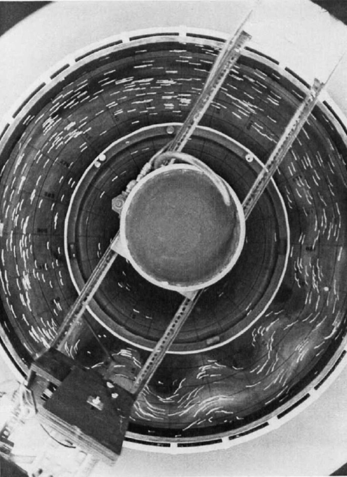
Stationary Rossby waves generated by an obstacle in a rotating annulus of liquid with a free surface. Adapted from Platzman (1968)
-
Moving some portion of the surface of the fluid container. This is commonly obtained by moving steadily or unsteadily one of the end walls of the annulus to produce an interior flow intermediate in velocity between the velocity of the two cylinders. One can create various inertial wave motions by either oscillating one of the cylinders (Firing and Beardsley 1976), or the whole container (Aldridge and Toomre 1969) or paddles inside the annulus (Ibbetson and Phillips 1967; Caldwell and Longuet-Higgins 1971).
-
Changing the speed of the tank rotation. Bringing the fluid in the rotating tank to a state of solid-body rotation, any small changes in the angular velocity of the tank can be seen as motion of the fluid with respect to the tank. However, this method is not very useful to obtain quantitative results since the basic flow is unsteady, it is a good technique for classroom demonstration.
-
Pumping fluid in/out of the interior. This is one of the oldest methods since it was used first by Stommel et al. (1958). Kuo and Veronis (1971) showed how disposing sources and sinks distributed along the sidewall and the Ekman layers produce a uniformly rising surface and a non-negligible solid-body azimuthal velocity. Later Baker (1971) simulated the small Ekman layer suction by pumping and sucking fluid through several holes drilled into one end plate of the rotating annulus.
-
Moving the whole fluid container. One can move the spin axis of the rapidly rotating container in some prearranged manner to study the fluid flow in precessing/nutating cavities. This technique can be used to explain some features of the geomagnetism of our planet (Malkus 1968).
-
Applying wind stress to the fluid surface. One can place fans and blowers to apply a stress to the free surface of a fluid as done by Von Arx (1952) to study the ocean circulation. This is another method that gives mainly qualitative results since we do not know neither the airspeed nor the value and distribution of the stress applied to the surface.
-
Deforming a part of the container. This technique can be applied to special situations such as studying tidal motions for instance (Suess 1970). Forced Rossby waves propagation can be studied also combining this technique with a rotating source-sink (Holton 1971).

2.2.2 Experiments: History
Experiments trying to reproduce at the laboratory scale the circulation in the atmosphere have been attempted long ago. The first ever examples were published in the nineteenth century by Vettin (1857, 1884). Vettin’s experiments only explored the regime that now we call the axisymmetric or “Hadley” regime since he did not observe clearly any instabilities such as the baroclinic instability (Hide and Mason 1975). Vettin’s experiments were followed some decades later by Exner (1923) in which it seems that the baroclinic instability was present. Exner observed clearly disordered and irregular flows due to the parameters range of this work but unfortunately also due to a lack of control of the key parameters. For more details about these pioneering works the reader is referred to the review by Fultz (1951).
In a similar period, Fultz at University of Chicago and Hide in Cambridge started independently a systematic series of experiments on rotating tanks (Fultz 1949; Hide 1958). Fultz’s set-up was constituted by the so-called “dishpan experiment”, i.e. a rotating fluid subject to horizontal differential heating in an open cylinder, see Fultz et al. (1959) for more details on his experiment series. Hide conversely worked with a heated rotating annulus focusing initially on the fluid motion in Earth’s liquid core (Hide 1969). Both researchers explored a vast parameter range elucidating the nature of several circulation regimes and laying the bases for successive research. Particularly they have unveiled the bifurcation and the paths to chaos in rotating flows and measured them using sophisticated non-invasive methods, such as using arrays of in-situ probes and optical techniques. It should be noted that their works show an overall agreement in identifying most of the features of circulation regimes and associating them to the correct dimensionless parameters space. The main discrepancy between them was the lack of a regular wave regime in Fultz’s open cylinder experiments, while in Hide’s annulus this regime was clearly visible. Despite some speculations that this regular wave regime could exist just in presence of an inner cylinder bounding the flow (Davies 1959), it was later shown that such a regime does exist also in flows rotating in open cylinder (Hide and Mason 1970; Spence and Fultz 1977). Furthermore, a remarkably accurate theory of the nonlinear behavior, e.g. mode selection, switching, vacillations, etc., observed in Fultz and Hide’s experiments was formulated by Lorenz (1962). The reader is referred to the detailed review written by Hide and Mason (1975) on the work conducted during this period.
The presence of persistent baroclinic wave flows is also a characteristic of another class of rotating stratified flows in which a two-layer stratification and a mechanically-imposed shear are present (Hart 1972). This experimental setup was introduced by Hart (1972) finding inspiration from the theoretical works of Phillips (1954) and Pedlosky (1970, 1971) on the stability of two-layer rotating flows. Hart’s configuration can be more easily compared to the theory than the thermally driven systems due to (i) the more straightforward way of introducing forcing and (ii) the absence of boundary layers which significantly reduce the flow complexity. Further extensive research on the two-layer setup have identified several forms of vacillation and chaotic behaviour (Hart 1979, 1985; Ohlsen and Hart 1989b,a) and how short-scale interfacial gravity waves can be excited through interactions with the quasi-geostrophic Rossby waves (Lovegrove et al. 2000; Williams et al. 2005, 2008).
In the last decades, very significant advances have been made by different groups around the globe on the experiments about (i) the classical axisymmetric instabilities of synoptic variability, (ii) vacillations, and (iii) the transition to turbulence. For example, the reader is referred to the works by the groups at Florida State University (Pfeffer et al. 1980; Buzyna et al. 1984), at Japanese universities (Ukaji and Tamaki 1989; Tajima and Kawahira 1993; Sugata and Yoden 1994; Tajima and Nakamura 2000; Tamaki and Ukaji 2003), at Oxford (Read et al. 1992; Bastin and Read 1997, 1998; Wordsworth et al. 2008), in Bremen/Cottbus (von Larcher and Egbers 2005; Harlander et al. 2011) and in Budapest (Jánosi et al. 2010). Furthermore, researchers have introduced the \(\beta \)-effect in rotating tank experiments through modifying the configuration to mimic the planetary curvature (Mason 1975; Bastin and Read 1997; von Larcher et al. 2013; Read et al. 2015a; Yadav et al. 2016) and zonally asymmetric topography (Leach 1981; Li et al. 1986; Bernardet et al. 1990; Risch and Read 2015). Very recently, Scolan and Read (2017) proposed a new experimental configuration to add the forcing thermal convection in the cylindrical rotating annulus through heating the bottom near the external wall and cooling the circular disk near the axis at the top surface of the annulus.
3 Theory of Rossby Waves
Theoretical background for Rossby waves has been developing over centuries (Hadley 1735; Laplace 1893; Hough 1897, 1898), however, clear physical sense of the waves was described by Rossby in his series of papers as a result of conservation of absolute vorticity (Rossby 1939, 1945).
In this section we will briefly review the basic theory of Rossby waves starting from simplest two-dimensional description.
General equations governing the adiabatic dynamics of a fluid in the rotating frame are the equations of momentum, mass continuity and energy
where \({\mathbf{v}}\) is the fluid velocity, \(\boldsymbol{\Omega }\) is the angular velocity of the rotating system, \(p\) is the fluid pressure, \(\rho \) is the fluid density, \(\gamma \) is the ratio of specific heats. Here \(\Phi =V_{1}+\Omega ^{2} r^{2}_{\perp }/2\), where \(V_{1}\) is the gravitational potential and \(r_{\perp }\) is the perpendicular distance from the axis of rotation. \(\nabla V_{1}\) can be also written as the gravitational acceleration, \({\mathbf{g}}\). Note that nonconservative forces are not taken into account in these equations. In the atmospheric science, the energy equation is often written for a temperature or an entropy, along with an equation of state.
The last term in the left-hand side of Eq. (6), \(2{\rho }\boldsymbol{\Omega }{\times }{\mathbf{v}}\), is the Coriolis force, a centrifugal force due to rotation, which plays a central role in rotating fluid dynamics. The force is named after G.G. Coriolis, who wrote the correct expression for this force for the first time and described it as a compound centrifugal force (Coriolis 1835). The force appears only in rotating systems and has three main properties: acts only on moving bodies, deflects the motion at right angles and does no work.
The ratio of the inertial to Coriolis accelerations given by
where \(U\) and \(L\) are characteristic velocity and length scales, is called the Rossby number (note that the Rossby number sometimes is also designated by \(\varepsilon \)). The Rossby number describes the importance of the rotation in the fluid dynamics: smaller Rossby numbers means that the dynamics is mostly determined by the rotational effects. Large-scale flows (with large \(L\)) lead to small Rossby number, therefore they are more significantly affected by the rotation.
3.1 Absolute and Potential Vorticity
The preeminent dynamic variable in fluid dynamics is the vorticity vector, \(\boldsymbol{\omega}\), defined as the curl of the fluid velocity
For uniformly rotating fluid the vorticity is \(\boldsymbol{\omega}= 2\boldsymbol{\Omega }\), which can be also called planetary vorticity. If we consider a rotating planet like the Earth, then the vertical component of the planetary vorticity is just Coriolis parameter
where \(\vartheta \) is the latitude. If we consider the fluid motion relative to the rotating system then the sum of planetary, \(2\boldsymbol{\Omega}\), and relative, \(\boldsymbol{\omega}\), vorticity is defined as an absolute (or total) vorticity
which is just the vorticity in an inertial frame.
Very important variable for the dynamics of Rossby waves is the potential vorticity
where \(\lambda \) is some quantity which is conserved during the fluid motion, i.e. \(d\lambda /dt=0\) (for two-dimensional barotropic flows \(\lambda \) is the \(z\) coordinate, while in the shallow water systems \(\lambda \) is the relative height with regards to the bottom). Taking the curl of Eq. (6) and using the continuity equation, Eq. (7), leads to the conservation of potential vorticity (Ertel 1942; Pedlosky 1987)
for barotropic fluids, \(\nabla \rho \times \nabla p=0\) or when \(\lambda \) is only the function of \(p\) and \(\rho \).
The conservation of potential vorticity leads to the appearance of Rossby waves. In dynamic shallow water systems, the potential vorticity can be rewritten as \(\Pi =(2\boldsymbol{\Omega}+\boldsymbol{\omega}_{0}+\boldsymbol{\omega})/H\), where \(\boldsymbol{\omega}_{0}\) is the vorticity related with background flows and \(H\) is the layer thickness. Spatial variations of each background vorticity i.e. planetary, \(2\boldsymbol{\Omega}\), and flow, \(\boldsymbol{\omega}_{0}\), vorticity as well as \(H\), may drive the Rossby-type waves. Latitudinal variation of the planetary vorticity is the historical prototype, therefore we will mainly concern with the planetary waves. However, the waves connected with the gradients of background flow vorticity and the layer thickness, will be also discussed in the section of astrophysical disks.
3.2 Hydrodynamic Rossby Waves
If the perturbation of gravitational potential is neglected, then Eqs. (6)–(8) are written after linearisation as
where \({\mathbf{v}}\), \(p^{\prime }\) and \(\rho ^{\prime }\) are small perturbations of velocity, pressure and density, respectively. \({\mathbf{U}}\), \(p_{0}\) and \(\rho _{0} \) are unperturbed values satisfying corresponding pressure balance. Here \(d/dt={\partial }/{\partial t}+({\mathbf{U}}{\cdot }{\nabla })\) is a material derivative.
Equations (15)–(17) are linear, but their solution is still complicated due to the vertical stratification of the real atmospheres and hence one can use some approximations. The simplest approximation is to consider homogeneous, incompressible purely horizontal motion (the “barotropic non-divergent” model). This is a model of prototype atmosphere and it provides the basic properties of the Rossby waves (Platzman 1968). The next step is to consider an incompressible fluid layer of uniform density, which is described by the shallow water approximation. The final step is to study the influence of stratification on the dynamics of the waves.
3.2.1 Two-Dimensional Rossby Waves
On two-dimensional isobaric (constant pressure) and isopycnic (constant density) surfaces the absolute vorticity, Eq. (12), is conserved by each fluid element i.e. \(d \boldsymbol{\omega}_{a}/d t=0\) leading to the appearance of two-dimensional Rossby waves.
We first consider that the spatial scales of perturbations are much smaller than the radius of the sphere. Then, the curvature is neglected and one can use the Cartesian coordinates \(x\) (directed prograde) and \(y\) (directed northward). Then the conservation of the absolute vorticity in incompressible fluids leads to the single equation
where \(U\) is the velocity of a homogeneous (generally prograde) jet, \(\psi \) is the velocity stream function (\(u_{x}=-\partial \psi / \partial y\), \(u_{y}=\partial \psi /\partial x\)). Expanding the Coriolis parameter, \(f\), at the given latitude \(\vartheta _{0}\) and retaining the lowest order latitudinal variation gives (Rossby 1939)
where
where \(R\) is the planetary radius. This is so-called \(\beta \)-plane approximation, which is widely used to describe the large-scale dynamics of the Earth’s atmosphere/oceans (Lindzen 1967; Gill 1982; Pedlosky 1987). The harmonic solution of Eq. (18) can be easily found as
where \(\sigma \) is the frequency and \(k_{x}, k_{y}\) are the wave numbers, which satisfy the dispersion relation
The zonal phase speed of the Rossby waves is (see Eq. (1))
where \(L\) is the wavelength. It is readily seen from Eqs. (22)–(23) that the frequency and longitudinal phase speed, \(c_{ph}=\sqrt{c^{2}_{phx}+c^{2}_{phy}}\), depend upon direction of phase propagation and wavelength. But the zonal phase velocity, \(c_{phx}\), is independent of the direction of the phase gradient and in absence of the jet (\(U=0\)) it is always directed to the west (retrograde), i.e., opposite to the rotation (note that the waves do not propagate strictly along latitudes, i.e., for \(k_{x}=0\)). This “retrograde drift” is the most charachteristic property of Rossby waves and it is related to the latitudinal variation of the Coriolis force. Figure 6 shows five patterns of plasma vorticity, initially at the same latitude in the northern hemisphere. If, randomly, two of them are moved poleward and one equatorward, then the two poleward-moved patterns will have increased relative vorticity and the equatorward-moved one will have decreased vorticity, due to the conservation of total vorticity. Thus, the poleward (equatorward) patterns will get an anticyclonic (cyclonic) relative vorticity. These anticyclonic/cyclonic motions will tend to move the other two undisturbed patterns and will change their vorticity. This vorticity will tend to restore the three patterns (first, third, and fifth patterns) back to their original position. Thus, a wave pattern will be formed and will move westward.

Illustration of retrograde drift of Rossby waves due to the conservation of absolute vorticity. Starting from five plasma flow patterns, initially at the same latitude, the first and the fifth patterns are moved poleward and the third equatorward (panel (a)). Due to conservation of vorticity, the first and the fifth patterns will have an anticyclonic (clockwise in northern hemisphere) and the third pattern a cyclonic relative vorticity (panel (b)). As a result, all five patterns will move in the direction shown by vertical arrows in panel (c), forming a westward-moving wave pattern. The figure is reproduced from Dikpati et al. (2018b) by permission of the AAS
Existence of the jet (\(U\neq 0\)) crucially affects the phase propagation of Rossby waves. There is a critical wavelength for each value of jet defined as
When the wavelength is larger (shorter) than the critical value then the waves propagate in retrograde (prograde) direction of rotation, respectively. When the wavelength equals to \(L_{c}\) then the waves become stationary, i.e., they do not propagate with regards to the Earth.
The components of the group speed of Rossby waves are
It is evident that the zonal group speed is prograde for \(k_{x}>k_{y}\) and retrograde for \(k_{x}< k_{y}\) in the absence of the jet. Therefore, for purely zonal propagation, the energy of wave packet propagates exactly opposite to the phase speed i.e. in the direction of rotation.
For sufficiently large-scale perturbations the Earth’s curvature should be taken into account. Haurwitz (1940) considered the conservation of absolute vorticity in spherical coordinates \(\theta , \phi \), where \(\theta \) is the colatitude increasing southward and \(\phi \) is the longitude increasing eastward. Using the stream function \(\chi \) defined as
the absolute vorticity conservation leads to the single equation for \({\mathbf{U}}=0\) (note that Haurwitz (1940) additionally considered homogeneous zonal flow)
One can assume that
which allows to obtain the associated Legendre equation (see also Longuet-Higgins 1964)
When \(2m\Omega /\sigma =-n(n+1)\), then this equation has bounded non-singular (at poles i.e. \(\theta =0, \pi \)) solutions in terms of associated Legendre functions, \(P^{m}_{n}(\cos \theta )\), \(Q^{m}_{n}(\cos \theta )\), where \(n=1, 2, 3. \dots\). This condition leads to the dispersion relation of Rossby waves (see Eq. (4))
Each solution with fixed \(n\) and \(m \neq 0\) (\({\lvert m \rvert }< n\)) has \(n-{\lvert m \rvert }\) zeros between the poles. They are called tesseral harmonics. If \(m=0\) then there is no nodal meridians and the solutions are zonal harmonics (or ordinary Legendre polynomials). When \(n={\lvert m \rvert }\) then there are no nodal parallels and solutions are sectoral harmonics.
3.2.2 Rossby Waves in Shallow Water Approximation
Two dimensional horizontal dynamics generally catches most properties of planetary waves, therefore these waves are sometimes called Rossby-Haurwitz waves. However, consideration of vertical density stratification is necessary for the complete description of wave dynamics. For small Rossby number, the vertical distribution of pressure will be only slightly disturbed from its static form which leads to vertically hydrostatic assumption for geophysical and astrophysical flows. The next approximation to take into account the vertical motion is shallow water theory. Shallow water model has been used to study the atmospheric and ocean dynamics on the Earth starting from tidal theory of Laplace (1893).
The shallow water approximation considers a shallow fluid layer of uniform density. This approximation can be safely used if the thickness of the layer is smaller than the density scale height. Laplace tidal equations for small perturbations can be written in the spherical coordinates (see previous subsection) as (Love 1913)
where \(H\) is the equilibrium thickness of the layer (which in principle can be nonuniform) and \(\eta (t, \theta , \phi )\) is the elevation. Here the perturbation of gravitational potential and external forces are neglected. The fluid is considered to be incompressible and inviscid. The scaling of the equations implies that the horizontal velocities remain independent on radial coordinate if they are initially. Divergent-free condition means that the radial velocity is linear function of radial coordinate inside this shallow layer. Pressure at any point is equal to the weight of the unit fluid column above that point at this instant. Fundamental parametric condition of shallow water approximation is
where \(L\) is the horizontal scale of perturbations.
To study the general properties of Rossby waves in shallow water approximation it is useful to consider first the Cartesian coordinates. In this case, Eqs. (31)–(33) can be rewritten as (e.g. Longuet-Higgins 1965)
where \(x\) and \(y\) are directed prograde and northward, respectively and \(f=2\Omega \sin \vartheta \). \(\theta \) and \(y\) are directed in opposite directions, which results in opposite signs in front of the Coriolis terms in Eqs. (31)–(32) and Eqs. (35)–(36).
These equations can be easily cast into the single equation
where
is the surface gravity speed. This equation has high-frequency and low-frequency solutions. High-frequency solutions are surface gravity waves and the low-frequency solutions are Rossby waves. In order to exclude the high-frequency waves from consideration, one has to neglect the term with third derivative of time, retaining only the Rossby waves. Then the solution of Eq. (38) depends on considered latitudes.
Away from the equator, \(\beta y \ll f_{0}\) in the Eq. (19), therefore, \(f^{2} \approx f^{2}_{0}\) and the plane wave analysis on \(\beta \)-plane leads to the dispersion relation (for \(\sigma/f_{0} \ll 1\))
The dispersion relation is very similar to the two-dimensional case – Eq. (22). The only difference is the last term in denominator, \(f^{2}_{0}/c^{2}\). This term is related with the Rossby radius of deformation
which describes relative importance of rotation with regards to the buoyancy effects. Note that \(R_{D}\) is an external radius of deformation, while for stratified fluids an internal radius of deformations is used (see the Sect. 3.2.3). When horizontal scale of perturbations is much smaller than the Rossby radius of deformation (\(k_{x} , k_{y} \gg R^{-1}_{D}\)), then Eq. (40) is completely transformed into Eq. (22).
The zonal phase speed of shallow water Rossby waves is
The frequency and longitudinal phase speed depend upon direction of phase propagation and wavelength, but the zonal phase velocity is independent of the direction of the phase gradient and it is always prograde i.e. opposite to the rotation.
Near the equator, \(f \approx \beta y\) and after Fourier analysis with \(\exp (-i\sigma t + i k_{x} x)\) Eq. (38) is transformed into the equation (Matsuno 1966)
This is the equation of parabolic cylinder (also known as the equation of quantum harmonic oscillator) and it has the bounded solutions
where \(H_{\nu }\) is a Hermite polynomial of order \({\nu }\) and \(C\) is a constant, which implies the dispersion relation (Matsuno 1966)
Polynomial order \(\nu \) corresponds to the poloidal wavenumber and defines the number of zeroes from north to south. The solutions are oscillatory inside the interval
where \(L_{e}=\sqrt{{{c}/{\beta }}}\) is the equatorial deformation scale, and exponentially tend to zero outside. The turning points or critical latitudes are defined by \(y/R=\sqrt{{{(2{\nu }+1)}/{\sqrt{\epsilon }}}}\), therefore when the Lamb parameter is large (\(\epsilon \gg 1\)), then the solutions are confined near the equator. The dispersion relation Eq. (45) describes several different wave modes. For \(\nu \geq 1\) there are low and high frequency waves. For the lower frequency waves the dispersion relation can be approximated as
These are equatorially trapped or equatorial Rossby waves as discussed at the end of the Sect. 2.1. The higher frequency waves are inertia-gravity waves, which are beyond the scope of the current review. When the wavelength of the equatorial waves is sufficiently large, so that \(k^{2}_{x} \ll (2{\nu }+1) \sqrt{\epsilon }/R^{2}\), then the dispersion relation of equatorial Rossby waves can be approximated by
so that the wave frequency depends on the surface gravity speed. For \(\nu =0\) Eq. (45) describes mixed Rossby-gravity waves (sometimes called the Yanai modes), which include westward propagating Rossby-gravity mode and eastward propagating inertia-gravity mode (Matsuno 1966). Note that the equatorial treatment also includes Kelvin waves, which have zero poleward velocities and formally described with \(\nu =-1\) in Eq. (45).
Now we turn back to the spherical coordinates. Considering the plane wave solution in the form of \(\exp (-i \sigma t+i m\phi )\), the Eqs. (31)–(33) lead to the single equation (Longuet-Higgins 1968)
where \(\mu =\cos \theta \), \(\lambda ={\sigma }/{2\Omega }\), \(u^{*}_{\theta }=i \sqrt{1-\mu ^{2}}u_{\theta }\) and
is the horizontal Laplace operator in spherical coordinates. This equation can be solved analytically by expansion in Legendre functions and using corresponding recurrent relations (Hough 1897, 1898). Particularly easy solutions can be found in the case of two extreme cases of the Lamb parameter, \(\epsilon \).
When the Lamb parameter is small, \(\epsilon \ll 1\), then for the Rossby waves (i.e. \(\lambda \ll 1\)) Eq. (49) is transformed into the equation (Longuet-Higgins 1965)
This is the spheroidal wave equation, those finite solutions over the whole range \(-1\leq \mu \leq 1\) are spheroidal wave functions, \(S^{m}_{n}(\sqrt{\epsilon }, \mu )\). The functions have \(n-m\) zeros over the interval \(-1< \mu < 1\) and tend to associated Legendre functions for \(\epsilon =0\). The tables of spheroidal wave functions and associated eigenvalues \(A^{m}_{n}=-m/\lambda \) can be found elsewhere (e.g. Stratton et al. 1956). Spheroidal wave functions and eigenvalues can be expanded as series of associated Legendre polynomials and power of \(\epsilon \), respectively. Then the dispersion relation for the Rossby waves for the lowest order of \(\epsilon \) can be obtained as (Longuet-Higgins 1965)
For \(\epsilon =0\) it is transformed into the dispersion relation of 2D Rossby waves (Eq. (30)) as expected.
When the Lamb parameter is large so that \(\epsilon \lambda \gg 1\), then for the Rossby waves (\(\lambda \ll 1\)) Eq. (49) leads to (Longuet-Higgins 1968)
where \(\xi =\epsilon ^{1/4}\mu \). This is the same equation as Eq. (43) and therefore leads to the equatorially trapped Rossby waves with the dispersion relation
The dispersion relation is identical with the dispersion relation in equatorial beta-plane, Eq. (48), where \(k_{x}\) is replaced by \(m/R\). Hence, spherical and rectangular geometries give the same dispersion relations for equatorially trapped Rossby waves.
3.2.3 Rossby Waves in a Stratified Fluid
In real situations fluids are stratified due to the gravity i.e. the density is vertically inhomogeneous. For complete description of Rossby waves, one should take into account the density stratification, which for small Rossby number is nearly hydrostatic. To uncover the properties of Rossby waves in stratified fluids, it is much easier to consider the beta-plane approximation. Linearised equation governing the dynamics of Rossby waves can be written as follows (Pedlosky 1987)
where \(S=N^{2}D^{2}/f^{2}_{0}L^{2}\) is the stratification parameter and \(\psi \) is the stream function. Here \(N=\sqrt{-g\rho '/\rho }\) is the buoyancy or Brunt-Väisälä frequency (′ sign means the derivative by \(z\)) and \(D\) is the vertical scale of motion. Stratification parameter can be also rewritten as \(S=L^{2}_{D}/L^{2}\), where \(L_{D}=N D/f_{0}\) is the internal deformation radius.
One can search the solution of this equation in the form of \(\psi (x,y,z,t)= \exp {i(-\sigma t +k_{x} x +k_{y} y)}{\tilde{\psi }}(z)\), where \({\tilde{\psi }}(z)\) is vertical structure function satisfying the equation
and corresponding boundary conditions. When \(l=l_{0}=0\) then the solution does not depend on vertical coordinate, which means that the horizontal velocities also do not depend on \(z\), while vertical velocity and density perturbations are zero. For nonzero \(l\) Eq. (55) is eigenvalue problem and may have infinite number of solutions, each associated with a real, discrete eigenvalue \(l_{j}\) (\(j=1,2,3,\dots\)). Inserting Eq. (56) into Eq. (55) the dispersion relation of Rossby waves can be obtained in the form of
Each \(\sigma _{j}\) is the frequency of the Rossby mode with corresponding \(l_{j}\). \(l_{0}=0\) solution corresponds to the barotropic mode, while \(l_{j} \neq 0\) solutions correspond to baroclinic modes. In all cases, this dispersion relation is identical to the dispersion relation of shallow water Rossby waves with homogeneous density Eq. (40) when \(l^{2}_{j}=f_{0}^{2}/c^{2}\), which can be also written as
where \(h_{j}\) is called the equivalent depth. Then, one can formulate a statement that the dynamics of \(j\)th Rossby-wave mode in a stratified fluid is identical with the dynamics of Rossby waves in a homogeneous layer, which has a depth \(h_{j}\). This theorem was derived by Taylor (1936) and it is valid for all wave modes in stratified and compressible atmosphere. Therefore, Rossby waves in stratified atmospheres can be modelled with shallow water equations with corresponding parameters. However, this statement is valid in completely spherical geometry. When the geometry differs from sphericity, then new properties of Rossby waves may arise and the corresponding modes are called quasi-toroidal modes or r-modes.
3.2.4 R-Modes in Stellar Interiors
Oscillation of a rotating fluid spheroid of finite ellipticity was first studied by Bryan (1889) considering incompressible Maclaurin’s spheroid which arises when a self-gravitating fluid body of uniform density rotates with a constant angular velocity. Bryan (1889) found the solution to this problem in terms of spheroidal harmonics and calculated oscillation periods of several harmonics with fixed wave numbers. Then Dahlen (1968) computed the normal mode eigenfrequencies of any Earth model which is slowly rotating, slightly aspherical and anisotropic.
To our knowledge the term r-mode for Rossby waves first was used by Papaloizou and Pringle (1978) in studying the non-radial oscillations of rotating stars and their relevance to the short-period oscillations of cataclysmic variables (binary stars, which consist of a white dwarf primary and mass transferring secondary, with irregular large variations of brightness). They estimated the correction to the Rossby waves dispersion relation, Eq. (30), due to the aspherical stellar form for high degree modes (in our notations \(n \gg 1\) modes). The authors found that the correction to the dispersion relation is small for the modes. Provost et al. (1981) studied the same problem in the approximation of slow rotation, \((\Omega /\Omega _{g})^{2} \ll 1\), where \(\Omega _{g}=\sqrt{GM/R^{3}}\) is the characteristic frequency of the star. Then the speed \(\Omega _{g} R=\sqrt{g R}\) is the surface gravity speed for the complete sphere and the parameter \(4(\Omega /\Omega _{g})^{2}\) is just Lamb parameter if one replaces \(H\) with the stellar radius, \(R\), in Eq. (5). They expanded the oscillation frequency
and all eigenfunctions in terms of small parameter \((\Omega /\Omega _{g})^{2} \ll 1\) and solved the basic HD equations for zero and first order approximations. In the zero order approximation, they obtained the Rossby waves dispersion relation (the authors used the term quasi-toroidal mode), Eq. (30) as expected and zero order eigenfunctions. Then they used these values to solve the equations in the first order approximation for the model of polytropic star (i.e. the star with polytropic pressure law). The eigenvalues (\(\sigma _{1}\)) and radial eigenfunctions have been calculated numerically for convective and radiative polytropes for first several lower order spherical harmonics. Resulted corrections due to the deviation from spherical symmetry were found to be significant, especially for the convective polytrope (\(\sigma _{1}\) reaching the value of 21.5 for the wavenumber of \(n=3\) and \(m=1\) in our notations, see the Table 2 in Provost et al. 1981). However, the correction to the Rossby wave dispersion relation, Eq. (30), is still negligible due to the smallness of expansion parameter, which for the Sun is estimated as \((\Omega /\Omega _{g})^{2} \approx 3 \cdot 10^{-6}\). Note that the perturbation of the gravitational potential is not considered neither by Papaloizou and Pringle (1978) nor by Provost et al. (1981). It has been shown, however, that taking the perturbations of the gravitational potential into account does not significantly affect the r-mode frequency (Smeyers et al. 1981; Saio 1982).
It is clear from the discussion that neither perturbations in gravitational potential nor the deviation from the spherical symmetry have significant influence on the properties of r-modes, therefore standard Rossby wave theory in stratified rotating fluids considered in the previous subsection is a quite good approximation for, at least, slowly rotating stars.
3.3 Magnetohydrodynamic Rossby Waves
Hydrodynamic description of Rossby waves is valid in the neutral atmospheres like on the Earth. However, astrophysical objects usually contain magnetic fields, which have important influence on the dynamics of Rossby waves. The magnetic Rossby waves were first studied in the context of the Earth liquid core (Hide 1966). Acheson and Hide (1973) wrote an excellent review about dynamics of rotating fluids with the presence of magnetic fields, where the influence of magnetic fields on Rossby waves have been intensively discussed. Gilman (2000) transformed Laplace tidal equations into magnetohydrodynamics (MHD) shallow water system for nearly horizontal magnetic fields, which are typical for the solar tachocline (a thin layer below the solar convection zone (Spiegel and Zahn 1992), where the solar dynamo magnetic field is presumably amplified).
In MHD, Eqs. (7)–(8) remain unchanged, while Lorentz force is added to Eq. (7), which now becomes
where \({\mathbf{B}}\) is the magnetic field strength and \(\mu _{0}\) is the magnetic permeability. The induction equation
which governs the dynamics of magnetic field strength, closes the system of equations (note that magnetic diffusion is neglected in the equation). Taking the curl of Eq. (60) shows that the absolute vorticity is no longer conserved owing to the presence of the Lorentz force.
3.3.1 Two-Dimensional Magnetic Rossby Waves
As in the hydrodynamic case, we start with the simplest two-dimensional problem on \(\beta \)-plane using the Cartesian coordinates \(x\) (directed towards rotation) and \(y\) (directed northward). Consideration of a uniform unperturbed magnetic field, \({\mathbf{B}}=(B_{x}, B_{y}, 0)\), and using the Fourier transform \(\exp (i k_{x} x +i k_{y} y-i\sigma t)\) leads to the following dispersion relation (Hide 1966; Gilman 1969c; Acheson and Hide 1973; Zaqarashvili et al. 2007)
where \({\mathbf{V}_{A}}={\mathbf{B}}/\sqrt{{\mu _{0}\rho }}\) is the Alfvén speed (the propagation speed of transverse displacements along magnetic field lines). For zero magnetic field, the dispersion relation transforms into the dispersion relation of \(\beta \)-plane Rossby waves, Eq. (22).
This equation has two solutions, therefore the magnetic field splits the ordinary Rossby mode into two different modes. The physical properties of the modes depend on the dimensionless parameter \(\gamma =2k^{2}({\mathbf{k}}{\cdot }{\mathbf{V}_{A}})/k_{x} \beta \) (Acheson and Hide 1973), where \(k^{2}=k_{x}^{2}+k_{y}^{2}\), which is the twice the ratio of Alfvén (\(\sigma _{A}={\mathbf{k}}{\cdot }{\mathbf{V}_{A}}\)) to Rossby (\(\sigma _{R}=k_{x} \beta /k^{2}\)) wave frequencies. When \(\gamma \gg 1\), i.e., strong magnetic field limit, then the two solutions transform into the solutions of Alfvén modes
which are slightly modified by the rotation. The waves propagating in the opposite direction of rotation have slightly higher phase speed than those propagating in the direction of rotation.
When \(\gamma \ll 1\), i.e., weak magnetic field limit, then the two solutions can be approximated as (Acheson and Hide 1973; Zaqarashvili et al. 2007)
The first solution is the HD Rossby wave dispersion relation, while the second solution corresponds to the dispersion relation of a new wave mode, which depends on both, the rotation and magnetic field strength. The second mode is called “hydromagnetic-planetary mode” (Acheson and Hide 1973) or “slow magnetic Rossby mode” (Zaqarashvili et al. 2007). Hence, the weak magnetic field splits the ordinary Rossby waves into fast (propagating opposite to the rotation) and slow (propagating towards the rotation) magnetic Rossby waves. We note that the frequency ratio \(\gamma \) can be very small for \(({\mathbf{k}}{\cdot }{\mathbf{V}_{A}})\rightarrow 0\), which does not necessarily require the weak field limit. Even small magnetic field component perpendicular to the rotation (in our case \(B_{y}\)) allows wave modes satisfying \(({\mathbf{k}}{\cdot }{\mathbf{V}_{A}})\approx 0\) condition to exist (the modes propagate almost perpendicular to the magnetic field). For these modes, the dispersion relation Eq. (62) governs HD Rossby waves while the slow magnetic Rossby waves are absent. The velocity perturbations for the modes with \(({\mathbf{k}}{\cdot }{\mathbf{V}_{A}})\approx 0\) are almost parallel to the magnetic field (because of their transverse nature), therefore the action of the Lorentz force is negligible. The solutions of Eq. (62) for different magnetic field strengths are plotted in Fig. 7. Left panels show the dispersion diagram of fast and slow magnetic Rossby waves for different magnetic field strengths when the poloidal magnetic field component is zero (\(B_{y}=0\)). Upper left panel corresponds to the weak magnetic field, which shows that fast magnetic Rossby waves follow the HD Rossby waves dispersion curves for small wavenumber, \(k_{x} R \leq 1\). At the same time slow magnetic Rossby waves differ from the corresponding Alfvén wave dispersion curve. For larger wavenumber, both magnetic Rossby waves tend to Alfvén wave dispersion curves as the increased magnetic tension suppresses the Coriolis force. For stronger magnetic fields (left middle and bottom panels), the magnetic Rossby waves tend to Alfvén wave solutions almost on all wavenumber range. Right panels show the dispersion diagram of fast and slow magnetic Rossby waves for same magnetic field strength, but now the poloidal magnetic field component equals the toroidal field so that \(B_{y}=-B_{x}\). It is clearly seen that when \(k_{x}=k_{y}\), which happens at \(k_{x} R=1\) (as we consider \(k_{y}R=1\)), the fast magnetic Rossby wave dispersion curve crosses the HD Rossby wave dispersion curve, while slow magnetic Rossby wave disappears. Hence \(({\mathbf{k}}{\cdot }{\mathbf{V}_{A}})= 0\) condition corresponds to the purely hydrodynamic case as was discussed above.

Dispersion diagram of fast and slow magnetic Rossby waves for different magnetic field strengths and directions for \(k_{y} R=1\). Left panels show the case of purely toroidal magnetic field \((B_{x} \neq 0, B_{y}=0)\), while the right panels show the case when the magnetic field has the angle of \(\sim45\) degree with the toroidal direction (\(B_{y}=-B_{x}\)). The upper, middle and lower panels correspond to the normalised Alfvén speed of \(V_{A}/2\Omega R=0.2\), 1 and 5, respectively. Red solid lines correspond to the fast magnetic Rossby waves. The Blue solid lines correspond to the slow magnetic Rossby waves. Red dashed lines correspond to the solutions of HD Rossby waves, while blue dashed lines correspond to pure Alfvén wave dispersion curves
Zonal phase speeds of fast and slow magnetic Rossby waves have simple expressions for the weak magnetic field approximation
respectively. The fast magnetic Rossby waves are always retrograde (i.e., they propagate in the opposite direction of rotation), while the slow magnetic Rossby waves are prograde (propagating in the direction of rotation). The zonal group speed has particularly interesting expression, which is obtained after differentiating Eq. (62) with respect to \(k_{x}\) (Hide 1966)
It is seen that \(({\mathbf{k}}{\cdot }{\mathbf{V}_{A}})= 0\) condition again leads to the HD zonal group speed. Additionally, if \(B_{y}=-B_{x}\) then the zonal group speed tends to zero for \(k_{x}=k_{y}\) harmonics. The poloidal group speed can be also readily obtained as
More of the physics of HD and magnetic Rossby waves can be demonstrated by computing fluid particle trajectories contained within a propagating wave. This involves integrating in time the solutions for horizontal velocities \(u_{x}, u_{y}\) for a given wave solution (Dikpati et al. 2020)
where \(A\) is an amplitude and \(n\) plays the role of wavenumber along \(y\) direction. These are coupled nonlinear equations in time, which are solved using an implicit method for calculating the fluid particle trajectory (see Dikpati et al. (2020) for details). The resulting trajectories for an HD Rossby wave and a fast magnetic Rossby wave of the same longitudinal wave length are shown in upper panel of Fig. 8. Both of these waves propagate to the left in the figure, that is, opposite to the sense of rotation of the system (retrograde). Figure 8 also illustrates that there can be both anti-clockwise and clockwise spirals in the trajectory of a fluid particle, depending on their starting point. Since the fast magnetic Rossby mode propagates retrograde faster than the HD wave, its spiral is more spread out. The latitude range of the spiral and the degree of overlap between adjacent spirals depends on whether the particle starts to move in a clockwise or anticlockwise part of the Eulerian streamline pattern. Lower panel of Fig. 8 shows a particle trajectory for the slow magnetic Rossby wave (prograde), for a disturbance of the same wavelength as in the previous figure. Being slow, the prograde spiralling trajectories of adjacent spirals strongly overlap. The same fluid particle traverses its trajectory before the wave pattern has moved very much, in contrast to what we see in the previous figure. Despite the differences just described, it is remarkable that qualitatively the particle trajectories in all these waves are quite similar.

Upper panel: particle trajectories in fast magnetic (solid curve) and HD (dashed curves) Rossby waves of same wavelength in \(x\) and same stream function amplitude, for both clockwise and anticlockwise flow starting points. If a particle starts from a point in the clockwise (or anticlockwise) flow, then it moves in a clockwise (or anticlockwise) spiral, represented in blue (or red) curves. Lower panel: particle trajectories in slow magnetic Rossby waves for strong toroidal magnetic field of 100 kGauss (\(a=1\) in nondimensional unit). Trajectories for two particles, the starting points of which are spaced a half wavelength apart (namely 0 and \(\pi \) in \(x\)), show clockwise (blue) and anticlockwise (red) spiralling prograde propagations. The figures are reproduced from Dikpati et al. (2020) by permission of the AAS
To study the magnetic Rossby waves in spherical coordinates is obviously more complicated even in the two-dimensional case. However, one gets easy solution for the toroidal magnetic field
where
This profile was first used by Malkus (1967) in studying the hydromagnetic planetary waves in rotating and stratified sphere. Using the Fourier analysis with \(\exp (-i\sigma t+im\phi )\) one can get the exact solution in terms of associated Legendre polynomials with the dispersion equation (Zaqarashvili et al. 2007)
As in the Cartesian geometry, there are two solutions of the dispersion equation corresponding to the fast and slow magnetic Rossby waves. The parameter \(\gamma \) now is proportional to \(\sim 2 n(n+1) V_{A}/(2\Omega R)\). For the strong magnetic field case, i.e. \(\gamma \gg 1\), there are two Alfvén-like modes propagating both in the direction of and opposite to the rotation with the same speeds.
When \(\gamma \ll 1\), i.e., weak magnetic field limit, then the two solutions can be approximated as
The higher-frequency solution, \(\sigma _{+}\), corresponds to the fast magnetic Rossby waves, which propagates opposite to the rotation and completely transforms into the HD Rossby waves for the zero magnetic field, Eq. (30). Therefore, this is the HD Rossby-Haurwitz mode modified by the magnetic field. The lower frequency solution, \(\sigma _{-}\), propagates in the direction of rotation and corresponds to the slow magnetic Rossby mode. The two solutions are exact spherical counterparts of rectangular magnetic Rossby waves, Eqs. (65)–(66). The zonal phase speed \(\sigma R/m\) does not explicitly depend on the toroidal wave number \(m\), which might suggest that the spherical Rossby waves are non-dispersive in the toroidal direction unlike to the Cartesian case. However, angular degree \(n\) is defined as the total number of zeroes on spherical surface, hence it automatically includes the variation along toroidal direction. Therefore, spherical Rossby waves are also dispersive as in the rectangular case.
To find the dispersion relations of magnetic Rossby waves is more complicated for other magnetic field profiles. Recently, Gachechiladze et al. (2019) found the dispersion relation of fast magnetic Rossby waves for the magnetic field profile
in the weak field approximation asFootnote 1
The field profile, Eq. (78), was first used by Gilman and Fox (1997) and it generally resembles the solar magnetic field having maximum at mid-latitudes and changing the sign at the equator. The dispersion relation is transformed into Rossby-Haurwitz formula, Eq. (30), in the nonmagnetic case. The dispersion relation of slow magnetic Rossby waves was not discussed in Gachechiladze et al. (2019), therefore it is an interesting problem in the future.
3.3.2 Rossby Waves in Shallow Water Magnetohydrodynamics
The next obvious step is to consider a shallow magnetised fluid layer with uniform density. The MHD shallow water equations for almost horizontal magnetic field were written by Gilman (2000) for the solar tachocline
where \({\mathbf{B}}\) and \({\mathbf{v}}\) are horizontal magnetic field and velocity, \(\nabla \) is the horizontal gradient, and \(H\) is the layer thickness.
The \(\beta \)-plane analysis away from equator leads to the dispersion equation for magnetic Rossby waves in the case of zonal uniform magnetic field, \(B_{x}=B_{0}\) (Zaqarashvili et al. 2007)
For zero magnetic field, the dispersion relation is transformed into the dispersion relation of the \(\beta \)-plane Rossby waves, Eq. (40). When \(k^{2} c^{2} \gg f_{0}^{2}, k_{x}^{2}V^{2}_{A}\), then the dispersion equation is transformed into the dispersion relation of two-dimensional magnetic Rossby waves, Eq. (62). The parameter \(\gamma \) is now written as
For the strong magnetic field (or \(\gamma \gg 1\)), the dispersion equation corresponds to the two Alfvén-like waves propagating in and opposite the rotation. For the weaker magnetic field (or \(\gamma \ll 1\)), the dispersion relations for the fast and slow magnetic Rossby waves can be approximated as
Fast magnetic Rossby waves propagate westward (opposite to the rotation), while the slow waves propagate eastward. Magnetic Rossby waves in the rotating channel of nonuniform height with horizontal magnetic field are also governed by similar equations (Zaqarashvili 2009). Vertical uniform magnetic field, \(B_{z}=B_{0}\), also leads to the same equation, Eq. (84), if one replaces \(k_{x}^{2}V_{A}^{2}\) by \(V^{2}_{A}/H^{2}\) (Heng and Spitkovsky 2009; Heng and Workman 2014). The influence of geomagnetic field on the dynamics of planetary waves in the Earth’s ionosphere has been also intensively studied (Khantadze et al. 2010).
Equatorial \(\beta \)-plane approximation for zonal uniform magnetic field results in the dispersion equation (Zaqarashvili 2018)
When the magnetic field is zero, the dispersion relation in the low frequency limit transforms into that of equatorial HD Rossby waves, Eq. (47). The remarkable difference with regard to the HD case is that the uniform toroidal magnetic field creates low frequency cut-off areas in the dispersion relation caused by the existence of \(k_{x}^{2}V_{A}^{2}\) term in the square root on the right hand-side. Hence the low-frequency magnetic Rossby wave, \(\sigma ^{2}< k_{x}^{2}V_{A}^{2}\), is no longer a solution of the dispersion relation: it is prohibited by the horizontal magnetic field through the action of the Lorentz force. The strong magnetic field opposes the vortex motion and prohibits the Rossby waves. Inhomogeneous magnetic field with the profile of Eq. (78), which can be approximated near the equator as \(B_{x} \sim B_{0} y/R\), produces interesting behaviour of equatorial magnetic Rossby waves. The dispersion relations for equatorial fast and slow magnetic Rossby waves can be approximated for small wavenumber as (Zaqarashvili 2018)
The equatorial fast magnetic Rossby waves have a similar dispersion relation to the HD equatorial Rossby waves for smaller wavenumber (because the magnetic field becomes very small in neighbourhood of the equator) and they propagate westward. Equatorial slow magnetic Rossby waves also propagate westward, which is opposite to the higher latitudes, where the slow waves propagate eastward (see Eq. 86). This point needs further detailed study. Dispersion diagrams of fast and slow magnetic Rossby modes from full dispersion equation with \({\nu }=1\) from Zaqarashvili (2018) are shown on Fig. 9. There is a cut-off region of fast magnetic Rossby waves for \(k_{x} R > 16.5\). The physical reason of the cut-off is not yet explained.

Dispersion diagram of equatorial fast and slow magnetic Rossby modes with \({\nu }=1\) vs normalised zonal wavenumber \(k_{x} R\). Here the Lamb parameter of \(\epsilon =4 \cdot 10^{3}\) and the magnetic field strength of \(B_{0}=10^{4}~\text{G}\) are used
Shallow water magnetic Rossby waves in the spherical geometry are more difficult to analyse. Márquez-Artavia et al. (2017) performed detailed analysis of the shallow water waves in the case of magnetic field profile Eq. (74). They found that the fast magnetic Rossby waves for the weak magnetic field and large Lamb parameter are equatorially trapped and can be expressed as
Hence the waves propagate westward similar to the HD case, but the slow magnetic Rossby waves propagate eastward (except anomalous \(m=1\) mode, which propagates westward). Márquez-Artavia et al. (2017) found that the fast and slow magnetic Rossby waves are trapped near the poles for the stronger magnetic field. The polar trapping of magnetic Rossby waves can also happen in the case of rapid rotation and/or reduced gravity (Zaqarashvili et al. 2009, 2011).
Density stratification due to the gravity may influence the dynamics of magnetic Rossby waves causing vertical structuring of the waves. Unfortunately, not much is currently known about the influence. Recently, Zeitlin (2013) showed that the shallow-water MHD model may be systematically derived by vertical averaging of the full MHD equations for the rotating fluid under the influence of gravity. Utilising similar scaling techniques and building on Gilman’s earlier pioneering work on magnetohydrodynamic modified quasigeostrophic flow (MQG, Gilman 1967a,c,b), Umurhan (2013) derived a set of model equations that is intermediate between MQG and shallow water MHD in a stably stratified atmosphere, arguing that this intermediate set of equations provide a conceptual framework to link MQG to MHD shallow water equations. In both instances, the procedures employed highlight the main approximations and the domain of validity of the two models, and allows for multi-layer generalisations and, hence, inclusion of baroclinic effects. This statement is similar to the theorem derived by Taylor (1936) for HD rotating systems (see Sect. 3.2.3). Certainly, much more can be done in exploring these directions in future. Furthermore, these equations may quite possibly be applied to the atmospheres of hot exoplanets, where the upper layers may be both sufficiently dense to be a fluid and ionised to be described by MHD processes.
3.4 Instability of Rossby Waves
Shear flow or differential rotation could lead to the destabilisation of Rossby waves in certain conditions. The instability conditions are similar to Rayleigh (Rayleigh 1880) and Fjørtoft (Fjørtoft 1953) conditions and/or to Howard semi-circle theorem (Howard 1961). In this subsection we review the basic properties of Rossby wave instability in plane-parallel shear flows. The instability of magnetic Rossby waves on differentially rotating spherical surface is briefly reviewed in Sect. 4.2.5.
3.4.1 A Minimal Model for Rossby Wave Instability
In this section we would like to provide a minimal model for the essence of the mechanism by which Rossby waves interact in a distance to perform instability. For clarity we then demonstrate the mechanism on the simple configuration of the Rayleigh model, where the Rossby waves are concentrated into two delta functions and then compare it with a more realistic scaled hyperbolic tangent shear layer. The two Rossby wave interaction paradigm was shown to be applicable for baroclinic instability (Heifetz et al. 2004) and to MHD shear flow dynamics (Heifetz et al. 2015), hence relevant to astrophysical setups.
In their seminal paper, Hoskins et al. (1985) presented a heuristic minimal model for barotropic shear instability based on the interaction at a distance between two counter-propagating Rossby waves. This model has been formulated mathematically by Heifetz et al. (1999) for the simple barotropic model of Rayleigh (1880) and by Davies and Bishop (1994) for the simple baroclinic model of Eady (1949). Later on, Methven et al. (2005) showed that this minimal model catches, surprisingly well, the essence of the instability of realistic atmospheric jets with complex baroclinic-barotropic structures. Heifetz et al. (2015) generalised then this model for magnetohydrodynamic shear flows to include the instability mechanism of mixed Rossby-Alfvén waves. Here we review this minimal model in a simple generalised from, based on the recent paper by Heifetz and Guha (2019).
The schematic picture of the interaction in its simplest form can be drawn as follows. Consider a 2D shear flow profile, plotted in Fig. 10, in the \((x,y)\) plane. The mean flow \(U(y)\) is pointing only in the \(x\) direction but the speed varies with \(y\). Furthermore, \(U(y)\) is positive in region I and negative in II. The vorticity, \(\Omega \), for a 2D flow is a scalar and for this shear flow profile, \(\Omega (y) = -dU/dy\) is non-positive everywhere. Its cross-stream derivative however, \(d\Omega /dy = -d^{2}U/dy^{2}\), is positive in region I and negative in II. Such flow satisfies the two celebrated necessary conditions for shear instability Rayleigh (1880) and Fjørtoft (1953). The Rayleigh inflection point criterion requires that the mean vorticity’s cross-stream derivative changes sign within the shear region, whereas the Fjørtoft condition has an additional requirement – the signs of the cross-stream vorticity derivative and the mean flow should be positively correlated. In our case, both fields are positive in region I and negative in region II, thereby satisfying Fjørtoft’s criterion in addition to Rayleigh’s criterion.

Schematic of interacting vorticity waves in a shear flow. A hyperbolic tangent shear layer, and the corresponding vorticity gradient profile are shown on the left-hand side. On the right-hand side, the cross-stream displacement, the associated cross-stream velocity and the associated sign of vorticity for each wave are shown, and represented by the same colour. Position of each undulating material line after a short time interval is shown by dashed line. Interaction leads to an additional cross-stream velocity (shown by a different colour). Note that cross-steam velocities due to undulations of the other material line are weaker (represented by shorter arrows) than those due to the self-induced vorticity anomalies. The horizontal arrow associated with a wave indicates the intrinsic wave propagation direction. Both waves are counter-propagating, i.e. moving opposite to the background velocity at that location. Adapted from Heifetz and Guha (2019)
The Rayleigh and Fjørtoft conditions were derived originally for normal mode instability and only in 1985 (Hoskins et al. 1985) were related to the more general constants of motion in linearised dynamics of pseudo-momentum (or equivalently wave-action, for monochromatic waves) and pseudo-energy, respectively. In that seminal paper, the authors provided a minimal model as well to rationalise these conditions, as is illustrated below. In a 2D inviscid, incompressible flow, a fluid element with the velocity field \({\mathbf{u}} = (u,v)\) materially conserves its vorticity, \(\tilde{q} = \partial v/\partial x - \partial u/\partial y\), as it moves. Since in region I the cross-stream derivative of the mean vorticity is positive, a fluid element that is displaced southward (in the negative \(y\) direction) conserves its relatively high vorticity and consequently develops a positive vorticity anomaly, \(q\), which induces a counter-clockwise circulation. Similarly, a fluid element that is displaced northward develops a negative vorticity anomaly with clockwise circulation. Thus, an undulated sinusoidal material line in region I (indicated by the grey solid line in Fig. 10) will tend to propagate to the west (in the negative \(x\) direction, the dashed grey line), counter to the mean flow \(U\), because the induced cross-stream velocity will shift fresh vorticity anomalies to the left of the existing ones.
Applying the same logic to region II, an undulated sinusoidal material line here will propagate to the east (black solid and dashed lines in Fig. 10), counter as well to the mean flow there. These shear Rossby waves are the building blocks of the minimal model. The sign of the cross-stream mean vorticity gradient determines the direction of their intrinsic phase speed. Therefore, when the Rayleigh’s criterion is satisfied, the waves propagate counter to each other, and when the Fjørtoft condition is satisfied as well, the waves also propagate counter to their local mean flow. Consequently, despite the mean shear, and even in the absence of interaction between the waves, the difference between the waves’ phase speeds is relatively small.
The second essential ingredient in this minimal model is the interaction at a distance between those building blocks. While the waves’ vorticity fields are localised, the velocity field attributed to each vorticity field is non-local by nature and decays away from each vorticity wave. Consequently, the two waves can interact at a distance by inducing on each other their individual cross-stream velocities. If the two waves’ vorticity fields are in phase (Fig. 11(a)), their cross-stream velocity will be in phase as well. Therefore, the induced velocity of one wave on the other will “help” the latter to translate its displacement faster and as a result, each wave will be propagating faster counter to its mean flow. In contrast, if the vorticity of the waves is in anti-phase (Fig. 11(b)), the waves will hinder each other’s counter-propagation rate. If the upper wave’s vorticity lags the lower one by a quarter of a wavelength (so that the waves are \(\pi /2\) out of phase), the far field velocity induced by each wave will not affect the propagation rate but will amplify the waves’ displacements. As each wave’s displacement amplitude is tied to its vorticity, increase in the vorticity amplitude of one wave will lead to an amplification of the vorticity amplitude of the other wave. Therefore, this scenario describes a mutual instantaneous amplification at a distance (Fig. 11(c)). In contrast, if it is the lower wave’s vorticity which is lagging the upper one by a quarter of a wavelength, the waves will mutually decay each other’s amplitudes (Fig. 11(d)). Generally, any setup of phase difference between the two waves yields mutual interactions that affect both on the waves’ amplitudes and the waves’ propagation rates (Fig. 11(e)). Figure 10 demonstrates a configuration where the waves amplify each other’s amplitude but hinder each other’s counter-propagation rate.

Schematic description of the linear interactions between counter-propagating vorticity waves. The waves depict interfacial displacement, while the horizontal and vertical arrows respectively denote stream-wise (background) and cross-stream velocities. Note that cross-steam velocities due to undulations of the other material line are weaker (represented by shorter arrows) than those due to the self-induced vorticity anomalies. (a) Fully helping, (b) fully hindering, (c) fully growing and (d) fully decaying configurations. (e) Depending on the phase difference \(\epsilon \) between the vorticity perturbations at the upper and lower undulating material lines, different kind of linear interactions can be expected, as shown by the “concentric circles”. The locations where the configurations (a)–(d) occur have been marked. The configuration given in Fig. 10 lies in the second quadrant (shaded in gray), which is the “growing-hindering configuration”. Adapted from Heifetz and Guha (2019)
The wave interaction picture described above can be translated into a generic set of equations constructing the minimal model. Denote the vorticity waves’ anomaly in the two regions as \(q_{1,2}(t)\) (indices 1 and 2 correspond to the two regions), and writing them in terms of their amplitudes and phases \(q_{1,2} = Q_{1,2}e^{i \epsilon _{1,2}}\), we obtain (Heifetz et al. 2004):
Consider first Eq. (91), which relates to the inner circle of Fig. 11(e) and describe the instantaneous growth or decay of the wave amplitudes due to the interaction at a distance. The relative phase of the waves is \(\epsilon \equiv \epsilon _{1} - \epsilon _{2}\), while the interaction at a distance coefficients, \(\sigma _{1,2}\) depend on the details of the problem. Note that \(\sigma _{1}\) is determined by the evanescent structure of the cross-stream velocity of wave 2, the effective distance between the two waves and the cross-stream mean vorticity gradient in region I (where equivalent arguments are implied for \(\sigma _{2}\)). It indeed indicates that \(\epsilon = \pi /2\) (Fig. 11(c)) is the optimal phase for mutual instantaneous amplification. Equation (92) relates to the outer circle of Fig. 11(e). The frequencies of the waves, \({\hat{\omega }}_{1,2}\), in the absence of interaction include both the effects of advection by the mean flow, \(U_{1,2}\) (which provides the Doppler shift) and the counter-propagation rate (which is the intrinsic frequency). The frequency of each wave can be either positive or negative. Positive values of \({\hat{\omega }}_{1,2}> 0\), indicate eastward wave propagation (in the positive \(x\) direction) in the absence of interaction, where the minus sign in front of them, at the RHS of Eq. (92), is because the waves’ phases increase when they propagate westward. Thus, when the waves’ vorticity fields are in phase (\(\cos {\epsilon }=1\), see Fig. 11(a)), the waves help each other to counter-propagate in agreement with the plus and minus signs in the last terms of Eq. (92) (Note that in Fig. 11, the displacement fields have been plotted. In Fig. 11(a) the displacement fields are anti-phased however the vorticity fields are in phase). The same logic can be applied for \(\epsilon = \pi \), Fig. 11(b), where the waves hinder each other’s propagation rate. The detailed dynamical properties of the Rossby wave interaction system can be found elsewhere (Heifetz et al. 2004; Heifetz and Guha 2018; Guha and Lawrence 2014; Pikovsky et al. 2001). Recently, the effect of finite Rossby radius of deformation on the Rossby wave interaction was analysed by Biancofiore and Umurhan (2019). They found that the two Rossby waves lose their counter-propagative character for small values of the Rossby radius of deformation. Thus, a less hindering, or eventually helping, configuration is needed to phase lock.
3.4.2 Application to the Rayleigh Model of Shear Instability
We wish to provide a concrete example for the wave interaction mechanism. One of the simplest setups for shear instability has been suggested by Lord Rayleigh in 1880 (Drazin and Reid 2004) for a piecewise version of the shear profile in Fig. 10:
Detailed analysis of the problem in terms of wave interaction can be found in Heifetz et al. (1999) for modal instability, and in Heifetz and Methven (2005) for non-modal growth. Here we note that for this piecewise version of shear profile the mean vorticity gradient is concentrated in \(y = \pm 1\):
Thus, the two vorticity waves are interfacial so that the perturbation vorticity \(q\) satisfies:
where \(k>0\) denotes the stream-wise wavenumber.
The instability growth rates for the piece-wise linear and the mixing layer continuous profiles are plotted in Fig. 12(a), whereas the vorticity and the stream-function structures of their most unstable modes are plotted in Fig. 12(b, c), respectively.

(a) Dispersion relation i.e. growth rate vs wave number for Rayleigh (grey) and scaled hyperbolic tangent shear layer (black). (b) Normalised perturbation vorticity for Rayleigh (black and white contour lines; black denotes positive and white denotes negative) and scaled hyperbolic tangent shear layer (filled coloured contours). (c) Normalised perturbation stream-function following the same colour as in panel (b). Adapted from Heifetz and Guha (2019)
3.4.3 Multi-wave Interactions
The interaction between the two vorticity waves, described in previous subsection, can be generalised straightforwardly to the case of \(N\) number of interacting waves, as is illustrated schematically in Fig. 13, and explained in Heifetz et al. (2009) for Rossby waves and in Heifetz and Guha (2018) for gravity waves. Multiple vorticity waves are located in concave and convex regions where the mean cross-stream vorticity derivative have local extrema. The cross-stream velocity field at every level is now composed of the in-situ velocity field, induced by the wave located at that level (indicated hereafter by the index, \(i\), and the contributions of the far field velocity induced by all of the other remote waves, indicated generally by the index, \(j\)). Naturally, the magnitude of the induced velocity decreases with the distance according to the evanescent structure of the Green function, which translates the vorticity source to the far field velocity field it induces. This structure is determined by the details of the problem setup (cf., different examples in Heifetz and Methven 2005) however it only depends on the cross-stream distance between waves \(i\) and \(j\). In the following formulation \(G_{ij}\) represents the Green function induced by a remote wave \(j\) on an in-situ wave \(i\). Since only the distance between the two waves matters for \(G\), it is symmetric, i.e., \(G_{ij}=G_{ji}\). Generally, we may expect that adjacent pairs of vorticity waves will affect each other more pronouncedly than remote pairs. Nonetheless, a remote vorticity wave with a large amplitude \(Q_{j}\) may affect a distant wave more strongly than a closer neighbour wave with a smaller amplitude.

Furthermore, as illustrated in Figs. 10 and 13 the cross-stream velocity field acts directly on the wave displacement. Thus, if the displacement and the vorticity wave anomalies are in phase (like in wave “2” in Fig. 10) a positive far field cross-stream velocity, acting to amplify the wave displacement, is also amplifying the positive vorticity anomaly. In contrast, when the wave displacement and vorticity anomalies are in anti-phase (as in wave “1” in Fig. 10) such far field velocity will increase the negative value of the vorticity anomaly. The amount by which an induced velocity increases the vorticity amplitude of an in-situ wave depends on the restoring mechanism of the wave itself and is generally different for Rossby, gravity, capillary or Alfvén waves. As we are interested in the prototype of the interaction we therefore indicate this factor by \(\alpha _{i}\), which is positive when the displacement and the vorticity wave anomalies of wave \(i\) are in anti-phase and negative when they are in phase. Denote \(\epsilon _{ij} \equiv \epsilon _{i}-\epsilon _{j}\), and \(\sigma _{ij} \equiv \alpha _{i} G_{ij}\), the generalisation of Eqs. (91)–(92) to \(N\) interaction waves read:
Thus, from this wave interaction perspective modal phase locking is achieved when a configuration is set to synchronise all waves to propagate with the same frequency: \(-\omega ^{*} = \lambda _{i}^{NM} ={\dot{\epsilon }}_{1} = { \dot{\epsilon }}_{2}=\cdots={\dot{\epsilon }}_{N}\), and to exhibit the same growth rate \(\lambda _{r}^{NM} = {{\dot{Q}}_{1}/ Q_{1}}= {{\dot{Q}}_{2}/ Q_{2}}=\cdots={{ \dot{Q}}_{N}/ Q_{N}}\).
3.5 Nonlinear Rossby Waves
Finite amplitude waves lead to the nonlinear phenomena, which may become of importance in different situations like wave steepening, wave-wave interaction, turbulence etc. We will briefly review two different aspects of nonlinear effects connected to Rossby waves: soliton solution and wave-wave interactions.
3.5.1 Rossby Soliton
Solitary waves or solitons arise when the nonlinear steepening of waves is balanced by the wave dispersion (Zabusky and Kruskal 1965). In this case, the steady structure is formed which propagates without change of form and properties. In the case of rotating shallow water system, a soliton can be formed as a nonlinear vortex monopole, which moves opposite to the rotation with slightly higher speed than the Rossby wave phase speed. The equation governing the nonlinear dynamics of shallow water layer with width \(H\) on a sphere rotating with angular velocity \(\Omega \) was derived by Petviashvili (1980)
where \(\eta \) is the elevation of the surface, \(r_{D}=c/f\) is the Rossby radius of deformation, \(v_{R}=c^{2}/f=c r_{D}\) is the phase speed of linear Rossby waves, \(\Delta \) is the Laplacian, \(\vartheta \) and \(\phi \) are the latitude and the longitude, respectively, \(J(\eta ,\Delta \eta )\) is the Jacobian of the functions \(\eta \) and \(\Delta \eta \). Derivation of this equation requires two assumptions that the wavelength of perturbations is much longer than the layer thickness, \(L \gg H\) (Eq. (34)), and that the time-scale of perturbations is much longer than the rotation period, \(d/dt \ll \Omega \). The second condition means that the approximation neglects surface gravity waves. This equation allows a steady state solution in the form of soliton (i.e., isolated vortex), \(\eta =h(\phi +u t/R, \vartheta )\), which satisfies the equation (Petviashvili 1980)
where \(-u\) is the soliton displacement speed along the longitude. Exact solution of Eq. (99) is not yet found. Petviashvili (1980) derived an approximate solution through expansion near the latitude \(\vartheta _{0}\) (similar to \(\beta \)-plane) as
where \(r\) is the distance from the soliton centre, \(L_{s}>r_{D}\) is the soliton radius and
is the expansion parameter. All the quantities of the soliton are determined by the characteristic radius of the soliton
The value of the longitudinal speed of soliton is directly proportional to the amplitude and inversely proportional to the soliton radius. Petviashvili (1980) obtained that the rotation of the vortex and the propagation direction are opposite to the rotation, hence the soliton is anticyclonic. The pressure in the vortex centre is higher than in the edges like in anticyclone.
Equation (99) is sufficiently general and can be applied to any latitude of the rotating sphere. The soliton solution has been found on the \(\beta \)-plane away from the equator by many authors (Williams and Yamagata 1984; Stegner and Zeitlin 1996; Tan and Boyd 1997). Numerical solution of the Petviashvili equation is presented on Fig. 14, which shows the propagation of stable structure in the opposite direction of rotation (Tan and Boyd 1997). The anticyclonic soliton propagates westward with slightly grater speed than the speed of long Rossby waves (Stegner and Zeitlin 1996; Tan and Boyd 1997). The Rossby soliton was also found in laboratory experiments (Antipov et al. 1981; Antonova et al. 1983), though they used the paraboloidal geometry, while the Petviashvili equation was derived in the spherical geometry (see discussion in Stegner and Zeitlin 1996). Rossby soliton solution on the \(\beta \)-plane may explain the basic properties of the Great Red Spot of Jupiter (see the Sect. 4).

Propagation of a soliton in the opposite direction of rotation. Here the contour lines of non dimensional surface elevation \(\eta /H\) is plotted. Here, the horizontal axis shows longitude and the vertical axis shows the latitude. Adapted from Tan and Boyd (1997)
On the other hand, Boyd (1980) obtained Korteweg-deVries equation for long, weakly nonlinear waves near equatorial region using the method of multiple scales. This equation permits the existence of equatorial Rossby soliton solution. Equatorial Rossby soliton has been subject to intensive study in the Earth’s context (Majda and Biello 2003; London 2017; Yano and Tribbia 2017).
Rossby soliton solutions have been discussed in many different aspects from planetary vortices to spiral galaxies (Nezlin et al. 1993). General problem of soliton stability was reviewed by Kuznetsov et al. (1986).
3.5.2 Nonlinear Wave-Wave Interactions
Waves with large amplitudes may interact with each other and lead to mutual energy exchange. The simplest process is the three-wave interaction when either one wave (pump wave) decays into two different waves or two waves merge into one wave through nonlinear interaction. Both momentum and energy must be conserved during the interactions, which leads to the following resonant conditions for two dimensional waves:
where \((k_{x1}, k_{y1}, \sigma _{1})\), \((k_{x2}, k_{y2}, \sigma _{2})\), and \((k_{x3}, k_{y3}, \sigma _{3})\) are wave numbers and frequencies of resonant waves (or resonant triad). In the case of Rossby waves, the wave numbers and frequencies must satisfy the dispersion relation, Eq. (22) (Longuet-Higgins and Gill 1967; Pedlosky 1987). Resonant interaction may also occur between different shallow water waves e.g. Rossby and inertial-gravity waves (Duffy 1974; Domaracki and Lossch 1977; Loesch and Deininger 1979; Eden et al. 2019). Hydrodynamic resonant decay has been recently generalised to the MHD shallow water wave-wave interaction where magneto-Rossby and magneto-inertial gravity waves take part (Raphaldini and Raupp 2015; Raphaldini et al. 2019; Klimachkov and Petrosyan 2016, 2017a,b). The ways that these nonlinear processes affect different astrophysical objects are still under investigation.
4 Rossby Waves in Astrophysical Objects
4.1 Rossby Waves in Solar System Planets
Besides the Earth, the Rossby waves were first observed on solar system planets, mostly on Jupiter and Saturn. This section summarises key observations of the waves in planetary atmospheres.
4.1.1 Jupiter
The Voyager spacecraft infrared, radio occultation, and imaging measurements provided an observational evidence for planetary-scale waves latitudinally trapped within Jupiter’s equatorial jet (Smith et al. 1979). The visually prominent plumes showed an organisation by longitudinal wavenumber 11–13 and have been interpreted as equatorially trapped Rossby waves (Allison 1990). Several years later, observations detected eight to nine longitudinal areas with high likelihood of containing a hot spot moving slowly westward. The wave numbers and phase speeds were found to be consistent with equatorial Rossby waves (Ortiz et al. 1998). Arregi et al. (2006) studied motion and spatial distributions of hot spots at \(7~^{\circ}\text{N}\) latitude of the Jupiter using 7 years observations at visible wavelengths between 1979 and 2002 combining the data of Voyagers 1 and 2, Hubble Space Telescope and ground based observatories. They estimated the velocity of spots as 97–113 m/s and zonal wave numbers as 6–20 (usually 8–12), which were interpreted as equatorial Rossby waves travelling along the planet and confined to upper troposphere. Comparing to the theoretical dispersion curves of the Rossby waves (obtained from the dispersion equation of Allison (1990), which is the same as Eq. (47)), the authors estimated the equivalent depth of the waves as 1–2 km and the background flow of 140 m/s (Fig. 15).

Comparison between the observed dispersion relationship measured from observed motions and wave number at the Jupiter (dashed lines) and the theoretical dispersion curves of equatorial Rossby wave (continuous line). Calculations for the meridional structure index \(j= 1\) (left) and \(j = 2\) (right) are shown, with different values of the equivalent depth of the Rossby wave, \(h\). The horizontal phase speed is measured relative to the background mean zonal flow velocity, which is a free parameter indicated between parentheses above each experimental (dashed) line. Adapted from Arregi et al. (2006)
Cassini reported an obvious signature of longitudinal wave pattern centered at \(14~^{\circ }\text{N}\) in both UV and near-IR brightness with a suggestion of the same wave in the cloud structures seen in the blue (Fig. 16). At its southern boundary, the zonal flow was moving at 100 m/s (eastward, i.e. to right), whereas at the northern boundary, the jet was retrograde with a velocity of \(-25~\text{m/s}\) (Porco et al. 2003). These observations were later interpreted as due to the Rossby waves (Li et al. 2006).

Three images of Jupiter (left) in blue (451 nm), (middle) in UV (258 nm), and (right) in the strong methane band (889 nm). A wave pattern, which circumnavigates the globe, is easily seen near \(14~^{\circ }\text{N}\) latitude in both UV and methane images (indicated by the arrow). It seems to be correlated with waves in the clouds seen at the same latitude in the blue image. The Great Red Spot is seen in the southern hemisphere of the planet. Adapted from Porco et al. (2003)
Both equatorial and high latitude Rossby waves have been frequently observed in the Jupiter atmosphere by the Cassini spacecraft, ground based and Hubble Space Telescope observations (Li et al. 2006; Barrado-Izagirre et al. 2008; García-Melendo et al. 2011; Simon-Miller et al. 2012; Legarreta et al. 2016).
Great Red Spot of Jupiter (see the spot in the southern hemisphere of the planet on Fig. 16) could be explained in terms of anticyclonic Rossby soliton solution (Petviashvili 1980; Williams and Yamagata 1984), which slowly moves in the direction opposite of rotation (see details in the Sect. 3.5). The spot shows slow westward drift of 1–5 m/s (Mitchell et al. 1981) corresponding to the barotropic soliton phase speed, however 3D numerical simulations revealed its deep baroclinic structure (Williams 1997). Recent Juno gravity measurements may shed light in the vertical structure of the Great Red Spot of Jupiter and in its physical origin.
4.1.2 Saturn
Saturn’s Polar Hexagon is the hexagonal, pole-centered cloud feature in Saturn’s northern atmosphere as revealed in Voyager close-encounter imaging mosaics. The hexagon has been interpreted as a stationary Rossby wave embedded within a sharply peaked eastward jet (of 100 meters per second), forced by the interaction of the jet with one or more adjacent anticyclonic ovals immediately to the south and meridionally trapped by the strong relative vorticity gradient of the flow itself (Allison et al. 1990). Cassini re-observed the long-term motion of Saturn’s north pole hexagon (Fig. 17) and has been again interpreted as a manifestation of a vertically trapped Rossby wave on the polar jet (Sánchez-Lavega et al. 2014).

Polar projected images of Saturn from the north pole to \(60~^{\circ}\text{N}\). (a) Composition of Cassini ISS CB2 images on 3 January 2009. (b) Cassini ISS RGB colour composition showing features in the hexagon and the jet stream on 26 August 2008. The red arrow marks the location of the hexagon. (c) Colour composite from 13–16 July 2013 obtained with the AstraLux camera on the 2.2 m telescope at Calar Alto Observatory (Spain). (d–f) Images obtained in 2013 by D.P. Milika (25 March), D. Peach (20 April), and C. Go (26 May), respectively. The figure is reproduced from Sánchez-Lavega et al. (2014)
Another remarkable structure in Saturn’s blue-red filtered images obtained by the Voyager spacecrafts is a ribbon; a dark wavy line (100 km across) encircling the planet at mid northern planetographic latitudes (at \(47~^{\circ }\text{N}\)) and moving with the peak of an eastward jet with velocity of 140 m/s. Sromovsky et al. (1983) measured the change in the ribbon’s Fourier phase spectrum over time and found a Rossby wave-like relation between the phase velocity and wavenumber of each Fourier component. Using images from the Cassini spacecraft, Gunnarson et al. (2018) recently analysed three ribbon waves in Saturn’s \(42~^{\circ }\text{N}\) eastward jet at \(45~^{\circ }\text{N}\), \(42~^{ \circ }\text{N}\), and \(39~^{\circ }\text{N}\) planetocentric latitudes (Fig. 18). They demonstrated that the morphology, wavelength, and propagation of the ribbon waves are consistent with barotropic Rossby waves with a smaller baroclinic component.

Morphology of the \(42~^{\circ }\text{N}\) jet as seen by Cassini ISS. (a) WAC CB2 mosaic, 13 January 2008. (b) WAC CB2 mosaic, 10 December 2012. (c) NAC CB2 image, 20 January 2012. (d) NAC MT2 image, simultaneous with (c). (e) NAC MT2 image, 5 May 2013. ISS = Imaging Science Subsystem; WAC = wide-angle camera; NAC = narrow-angle camera. East is to right. The figure is reproduced from Gunnarson et al. (2018)
Read et al. (2009) suggested that the longest Rossby waves could be frequently coherent across its adjacent jets and almost stationary relative to its bulk planetary rotation period on the basis of the atmospheric planetary-wave configuration (potential vorticity and zonal wind). Then they determined the rotation period of Saturn to be almost 5 min shorter (\(10~\text{h}\ \text{34}~\text{min}\ 13 \pm 20~\text{s}\)) than measured by Cassini spacecraft (\(10~\text{h}\ \text{39}~\text{min}\ 24 \pm 7~\text{s}\)). The semi-stationary character of Saturn’s Polar Hexagon might be related with adjustment of atmospheric flow towards a state of marginal dynamical stability as discussed by Read et al. (2009).
The observed 10.7 hour modulation of various phenomena in Saturns’s magnetosphere was recently explained by westward propagating Rossby waves (Smith et al. 2016).
4.1.3 Mars
Wave-like planetary-scale perturbations on Mars are found in the Mariner 9 IRIS atmospheric temperature data during late Northern Hemisphere winter in a latitude band between \(45~^{\circ }\text{N}\) and \(65~^{\circ }\text{N}\) (Conrath 1981). A suggested mechanism for the perturbations is that they are forced, quasi-stationary planetary waves that arise predominantly via zonally asymmetric surface properties (Hollingsworth and Barnes 1996). Later, Hinson et al. (2003) reported new observations of stationary planetary waves in the southern hemisphere of Mars with significant amplitudes at zonal wave numbers \(m = 1\) and 2. The geopotential field of the \(m = 2\) component was barotropic in character and can be modelled as stationary planetary waves.
4.1.4 Pluto
Observations of the 2007 March 18 occultation of the star P445.3 by Pluto resulted in light curves with unprecedented high signal-to-noise ratios, which revealed significant oscillations in the number density, pressure, and temperature profiles of Pluto’s atmosphere (Person et al. 2008). Detailed analysis of light curves indicated that these variations in Pluto’s upper atmospheric structure exhibit a previously unseen oscillatory structure with strong correlations of features among locations separated by almost 1200 km in Pluto’s atmosphere. Person et al. (2008) concluded that these variations are caused by large-scale atmospheric Rossby waves.
4.2 The Sun
The detection of Rossby waves is more complicated in other astrophysical objects like the Sun, stars or accretion/galactic discs. In recent years, however, the study of the waves is rapidly developing in the solar context. First of all, helioseismology can provide us with surface and internal velocity maps, which can be used to reconstruct the Rossby wave patterns. The Rossby waves can also influence solar magnetic fields and hence can be detected through solar magnetic activity variations.
First attempt to interpret observations in terms of Rossby waves on the Sun was made by Suess (1971), who reported the direct detection of the waves in global velocity field on the solar surface. However, this preliminary study remained unexpanded and the subject was not studied further until the new century, when Kuhn et al. (2000) have reported observations of a regular structure of 100 m “hills” uniformly spaced over the surface of the Sun with a characteristic separation of 90,000 km. They suggested that this structure is the surface manifestation of Rossby waves, or r-modes oscillations. However, several years later Williams et al. (2007) showed that the observation was a signature of super-granulation rather than Rossby waves. Therefore, the subject of direct detection of Rossby waves was again not discussed in literature until recent years, when attempts to detect the waves again revived. On the other hand, relation of Rossby waves to intermediate periodicity in solar activity has been the subject of continuous discussion during years. It must be clearly distinguished between direct and indirect detections of Rossby waves on the Sun. Measurement of velocity (helioseismic or granulation tracking) and longitude-dependent patterns of solar magnetic structures (coronal bright points or coronal holes) are direct methods to observe the Rossby wave characteristics (phase speed, wavenumber etc.). While the periodic variation in solar activity with Rossby wave time scales is an indirect method, though it may reveal an important information about the waves in the solar interior. This subsection reviews the theory and observations of Rossby waves on the Sun.
4.2.1 Evidence for Magnetic Rossby Waves in the Sun
Surges of magnetic flux emergence give rise to the quasi-periodic occurrence of flares (and CMEs) on the Sun’s magnetic activity bands at mid solar latitudes, as discussed in McIntosh et al. (2015). The surges are easily observed in the daily sunspot record, see panel A of Fig. 19. At latitudes above these activity bands, in the first few years of the descending phase of cycles, recurrent high-speed solar streams are observed (e.g., Legrand and Simon 1981). The source of these fast wind streams quasi-rigidly rotate. McIntosh et al. (2015) demonstrated the quasi-periodic nature of the fast solar wind speed and density. The coupling of these phenomena shows that the magnetic activity bands of the 22-year Hale magnetic cycle (those that comprise the present and upcoming sunspot cycles) are stacked in latitude, and are present on the solar disk almost all of the time (McIntosh et al. 2014).

Coronal EUV BP density Hovmöller diagrams derived from the combined observations of STEREO and SDO. We show the southern (Panel B) and northern (Panel C) activity bands with respect to the daily hemispheric sunspot number (Panel A). These BP density Hovmöller diagrams illustrate features of rising phase of sunspot cycle 24 and highlight, in particular, the rapid longitudinal growth of activity after the middle of February 2011 and strong correspondence between the enhanced density of the activity trains (drifting slowly from right to left) and global surges of flux emergence (as seen in panel A)
As discussed earlier (Fig. 1) a diagnostic to demonstrate the motion of the observed phenomena in longitude and connect it to the underlying process comes from the construction of a Hovmöller diagram (Hovmöller 1949). We remind the reader that the axes of a Hovmöller diagram are longitude (abscissa) and time (ordinate) for fixed latitudes. Combining the analysis of EUV images in the broadband channels taken by the twin STEREO/EUVI (195 Å) and SDO/AIA (193 Å) telescopes allowed to develop the 360 degree density map of coronal bright points (BPs; ubiquitous compact bipolar magnetic regions that have enhanced coronal emission above them, e.g., McIntosh and Gurman 2005; Madjarska 2019). The three spacecraft enabled imaging of the entire solar corona from February 6, 2011 until July 1, 2014.
The systematic analysis of the BPs present in the images of the three spacecraft permit the tracking of the magnetic activity bands of the 22-year magnetic cycle of the Sun (McIntosh et al. 2014). Visible in the panels of Fig. 19 are episodes of quasi-periodic small-scale magnetic flux emergence for comparison with the production of the sunspots seen in Panel A. McIntosh et al. (2017) used a BP detection algorithm on a series of coronal images taken by twin STEREO spacecraft and the SDO spacecraft and combined the detected BPs (at 4 hour cadence) across the solar sphere to construct latitude-longitude images of the BP density from which Hovmöller diagrams could then be constructed. Typically, due to their sparsity, these BP diagnostic maps are running averages over time and over a narrow range of latitudes, for panels panel B and C of Fig. 19 we show the evolution in circular bands that are centered on the latitude of the magnetic activity bands that gave rise to sunspot cycle 24. We see the rapid change in longitudinal behaviour in the activity bands as the sunspot cycle is initialised – this is most pronounced in the northern hemisphere (McIntosh et al. 2019). Note also the large periods of no activity before the slanted features start in both hemispheres and the clear asymmetry of magnetic activity between the southern (panel B) and northern (panel C) hemispheres in the short span of time depicted.
In mid-February 2011 there is an abrupt switch-on of activity in the northern hemisphere that over time begins to encompass more longitudes (McIntosh et al. 2019). Note that the southern hemisphere lags the north, but short episodes of activity are noticeable in longitude. McIntosh et al. (2017) measured the characteristics of the regions with enhanced BP density to capture the presence of two, oppositely directed velocities in the data as we have mentioned above; a slow \(\sim3~\text{m}\,\text{s}^{-1}\) westward (prograde) phase velocity, of individual clusters while analysing the apparent motion of clusters revealed a \(24~\text{m}\,\text{s}^{-1}\) eastward (retrograde) group velocity. These patterns can be explained by magnetic Rossby waves (see Sect. 3.3.1, Eqs. (68)–(69) for \(k_{x}< k_{y}\)). Furthermore, McIntosh et al. (2017) noted that the BP clusters exhibit lifetimes that are integer numbers of the rotational period at the latitudes sampled, hinting further that the processes governing the magnetic flux emergence underlying the signal was intrinsically tied to the rotation of the plasma.
Further, using Hovmöller diagrams constructed from the raw EUV images of STEREO and SDO, the lifetimes and propagation characteristics of coronal holes in longitude were studied (Krista et al. 2018) where three distinct populations of “low-latitude” (below \(65^{\circ}\) latitude) coronal holes were readily detected. One population rotates in retrograde direction and coincides with a group of long-lived (over sixty days) coronal holes in each hemisphere. These recurrent (from the perspective of the Sun-Earth line) coronal holes were located between \(30^{\circ}\) and \(55^{\circ}\), and displayed velocities of around \(55~\text{m}\,\text{s}^{-1}\), slower than the local rotation rate. A second, smaller population of long-lived coronal holes were observed inside \(10^{\circ}\) latitude – those exhibit prograde motion with velocities between 20 and \(45~\text{m}\,\text{s}^{-1}\). A third population of CHs exist that are short-lived (they live less than two solar rotations). They appear over a very wide range of latitudes and also exhibit a wide range of velocities (−140 and \(80~\text{m}\,\text{s}^{-1}\)). A butterfly diagram of the rising phase of sunspot cycle 24 showed a systematic evolution of the longer-lived holes at mid-latitudes, appearing to connect them with the overlapping band picture developed by McIntosh et al. (2014) and hinted at by Legrand and Simon (1981), but the sample was too short to draw concrete conclusions.
4.2.2 The Solar Convection Zone
Rossby waves are waves of radial vorticity and produce a distinct pattern in the horizontal velocity field at the solar surface. Various methods have been used to produce maps of horizontal flows at the surface and in the shallow near-surface layers of the Sun. We briefly review recently used methods to detect the Rossby waves.
Granulation Tracking
The method known as “granulation tracking” consists of following the motion of solar granules in the photosphere in consecutive images of the solar continuum intensity. Solar granules are bright convective cells with a typical size of 1500 km and a lifetime of several minutes, that act as tracers of the larger-scale flows in which they are embedded. SDO/HMI intensity images have sufficient spatial resolution (700 km at disk centre) and sufficient temporal cadence (45 sec) to be used for granulation tracking: granules do not evolve substantially from one image to the next and thus can be used as passive tracers of horizontal flows. After averaging these flows in time to reduce noise level, the radial vorticity can be obtained from the two horizontal components of the velocity. Löptien et al. (2018) used this method to obtain maps of the radial vorticity on the solar surface every 30 min since May 2010. These maps contain sufficient signal-to-noise ratio to study Rossby waves.
Helioseismology
Helioseismology is another method to measure flows in the upper convection zone. In helioseismology, line-of-sight velocity observations of solar acoustic waves at the surface are used to probe flows in the solar interior (Gizon et al. 2010).
Ring-Diagram Helioseismology
Ring-diagram analysis is a particular method of helioseismology that has been used to study solar Rossby waves. This method is based on measuring the local frequencies of solar acoustic modes; these frequencies are shifted by internal flows through the Doppler effect. Löptien et al. (2018) and Proxauf et al. (2020) applied ring-diagram helioseismology to SDO/HMI observations to map horizontal flows at different depths in the solar interior at a cadence of approximately one day. Maps of radial vorticity from helioseismology and granulation-tracking correlate very-well with each other at the largest spacial scales, thus implying that these maps contain little noise.
Time-Distance Helioseismology
Time-distance helioseismology is another method for measuring flows in the solar interior. It is based on extracting the travel times of solar seismic waves from two-point correlations in the observed surface wavefield. The larger the separation distance between the two surface points, the deeper the ray path connecting the two points. The travel times are perturbed by the presence of local subsurface flows. A travel time is reduced when seismic waves travel in the direction of the flow, while it is increased when the waves travel against the direction of the flow. Since vertical flows are much smaller than horizontal flows in the near-surface layers, the travel-time difference for waves traveling in opposite directions along the same ray path are proxies for horizontal flows in the interior (more sophisticated interpretations require inversion methods). Langfellner (2015) extensively explored the use of time-distance helioseismology for the measurement of radial vorticity near the solar surface. In particular, he showed that for intermediate and large scales, the near-surface radial vorticity inferred from \(f\) and \(p_{1}\) time-distance helioseismology is in excellent agreement with the granulation-tracking results. More recently, Liang et al. (2019) measured p-mode travel-time differences in the north-south direction in the low-latitude regions from 21 years of SOHO/MDI and SDO/HMI data. The acoustic ray paths that they used mostly probe the upper half of the convection zone. The longitudinally-varying north-south flows near the equator are diagnostics of the radial vorticity of the equatorial Rossby modes.
Evidence for Classical Rossby Waves in the Sun
Rossby waves were first identified in the Earth atmosphere as giant meanders in the northern hemisphere jet stream (see Sect. 2.1). These waves may exist in any rotating fluid (or plasma) body, including the Sun which rotates with a period of 25 days at the equator. Even though they were predicted to exist in the Sun and stars more than forty years ago (Papaloizou and Pringle 1978), they were unambiguously detected on the Sun only two years ago (Löptien et al. 2018). Classical Rossby waves leave their signature in maps of horizontal motions on the solar surface as patterns of radial vorticity that propagate in the direction opposite to rotation in the corotating frame. They are identified by a well-defined dispersion relation, Eq. (4).
The dispersion relation can be observed in Fourier space: The time series of radial vorticity maps at high cadence are Fourier-transformed in time and a spherical harmonic transform is applied with respect to the spatial coordinates. Löptien et al. (2018) discovered classical Rossby modes only in the sectoral (\(m=\ell \)) power spectra thus obtained. Notice that, in this section, we use the notation \(\ell \) to refer to the spherical harmonic degree (called \(n\) in the most of the rest of the paper). Löptien et al. (2018) only saw these equatorial Rossby modes very clearly for \(m\) values in the range \(3\le m \le 15\). Figure 20a shows a similar sectoral power spectrum of the radial vorticity at a depth of 9.9 Mm obtained by Proxauf et al. (2020) using ring-diagram analysis of SDO/HMI data. Peaks of power (see Fig. 20b for \(m=7\)) are seen at the resonant frequencies \(\omega = - 2\Omega /(m+1)\) in the frame rotating at the equatorial surface rotation rate \(\Omega \). This was confirmed by Liang et al. (2019) using time-distance helioseismology of north-south flows, by Hanasoge and Mandal (2019) using normal-mode coupling helioseismology, and by Alshehhi et al. (2019) using fast inversions of ring-diagram fit parameters. Recently, Hanson et al. (2020) confirmed the Rossby modes in GONG++ ground-based ring-diagram flow maps.

(a) Sectoral (\(\ell =m\)) power spectrum of the radial vorticity in the corotating frame as a function of longitudinal wavenumber, \(m\), and temporal frequency, \(\omega /2\pi \), from SDO/HMI ring-diagram helioseismology at a depth of 9.9 Mm for the period May 2010 to December 2017 (Proxauf et al. 2020). For clarity, the power in the plot is normalised at each \(m\) to the total power between −300 and 100 nHz. The blue solid line shows the theoretical dispersion relation \(\omega = -2\Omega /(m+1)\), where \(\Omega /2\pi = 453.1\) nHz is the equatorial rotation rate at the solar surface. The minus sign indicates a retrograde propagation. (b) Cut of panel (a) at \(m=7\). (c) Estimate of the latitudinal dependence of the eigenfunction for mode \(m=7\), obtained from the correlation of the mode’s radial vorticity between the equator and other latitudes
The horizontal eigenfunctions can also be measured from the observations by cross-correlating the vorticity signal for any particular mode between the equator and other latitudes (Fig. 20c). Horizontal eigenfunctions peak at the equator, but decay faster with unsigned latitude than sectoral spherical harmonics. Figure 21 shows a schematic representation of the radial vorticity of the solar Rossby modes with \(m=3\), 7, and 11.

Sketch of the radial vorticity of the equatorial Rossby waves observed in the solar near-surface layers by Löptien et al. (2018), for longitudinal wavenumbers \(m = 3\), 7 and 11. The red and blue patches indicate clockwise and counter-clockwise radial vorticity. In the corotating frame, the patterns propagate in the retrograde direction (to the left)
Mode Parameters: Frequencies, Lifetimes and Amplitudes
The parameters of the global-scale modes have been measured by several authors (Löptien et al. 2018; Liang et al. 2019; Hanasoge and Mandal 2019; Mandal and Hanasoge 2020; Proxauf et al. 2020; Hanson et al. 2020). The parameters of each mode (each \(m\) value) were extracted by fitting the Lorentzian function to the corresponding sectoral power spectrum (see, e.g., Fig. 22). The fits provide the mode frequency, mode linewidth (full width at half maximum), mode amplitude, and the background noise level. Table 1 shows a subset of the measurements of mode frequencies and linewidths. The mode frequencies are negative to indicate a retrograde phase speed. The frequencies are close to the classical dispersion relation for Rossby waves. The frequencies for the modes \(m=3\), 4, and 8 are close but different from the classical values by more than two \(\sigma \)s (about 25 nHz below for \(m=3\)). As shown by Liang et al. (2019), the \(m=2\) mode is not visible in the spectrum. Hanson et al. (2020) find that the mode frequencies from various authors are consistent with each other for the lowest \(m\) values, \(3\le m\le 7\). The mode linewidths are in the range from 20 to 50 nHz for most modes. For \(m=3\), the linewidth is very small with a value of 7 nHz measured by Liang et al. (2019) using 21 years of combined SOHO and SDO time-distance helioseismology data. The linewidths imply typical lifetimes of two to six months, with a maximum of about 1.4 year for \(m=3\). Löptien et al. (2018), Liang et al. (2019), and Mandal and Hanasoge (2020) measured the velocity amplitudes associated with each mode. These are of order 1 m/s, i.e. small in absolute value, but very significant in comparison to other motions (e.g., convection) at the same scales.

Power spectra of solar Rossby modes for different azimuthal orders \(m\) (black curves) from 21 years of north-south travel-time differences around the equator (Liang et al. 2019). The red curves are Lorentzian fits to the power spectra. Due to incomplete data coverage, there are leaks from modes with wavenumber \(m-1\) and leaks from very low frequency power (active region flows or convection) indicated by the purple and orange segments. Figure adapted from Liang et al. (2019)
Horizontal Eigenfunctions
The amplitudes of solar equatorial Rossby waves at each latitude can be estimated from the vorticity maps. Using a correlation technique, Löptien et al. (2018) and Proxauf et al. (2020) measured these horizontal eigenfunctions for each longitudinal wavenumber. They found that the eigenfunctions are maximal at the equator, change sign at latitudes around \(20^{\circ }\)–\(30^{\circ }\), and decay above this latitude (see Fig. 20c for the case \(m=7\)). These eigenfunctions differ from the sectoral spherical harmonics, which would be expected for modes in a uniformly rotating star. Recently, Proxauf et al. (2020) also measured the imaginary parts of the eigenfunctions, which are significantly non-zero for several modes. The imaginary part implies a small variation of the phase of the eigenfunctions with latitude. Recent work by Gizon et al. (2020) demonstrates that the decrease of the solar rotation rate with latitude plays a key role in shaping the Rossby wave eigenfunctions. In this work, they consider a parabolic shear flow in the equatorial \(\beta \)-plane to model solar differential rotation. In the inviscid case, the eigenfunctions are singular at critical latitudes such that \(U-c =0\), where \(c<0\) is the wave speed (retrogade in the corotating frame) and \(U<0\) is the shear flow measured from the equator in the corotating frame (\(U<0\)). In the presence of eddy viscosity, the singularities are removed and the eigenfrequencies are complex and discrete. For reasonable values of the viscosity, all modes are stable. At fixed longitudinal wavenumber, the least damped mode is a symmetric mode with a real frequency close to that of the classical Rossby mode. The real part of the eigenfunction has the same functional form as the one that is observed: its amplitude decays faster than the sectoral spherical harmonic function and switches sign near the critical latitude. Gizon et al. (2020) conclude that each longitudinal wavenumber is associated with a latitudinally symmetric Rossby mode trapped at low latitudes by solar differential rotation.
Radial Eigenfunctions
Observationally, little is known about the radial variations of the solar Rossby wave eigenfunctions. Proxauf et al. (2020) used ring-diagram analysis to study their amplitudes at different depths down to about 17 Mm in the interior. Above 7 Mm, the vorticity amplitudes increase with radius by about 10% to their surface values. The results below 7 Mm depend on distance from the central meridian, which indicates the existence of systematics and prevents a firm conclusion. Duvall et al. (2018) detected Rossby waves down to 70 Mm using deep-focusing time-distance helioseismology. In this depth range, the north-south velocity is consistent with an \(r^{m}\) dependence, with \(r\) the distance to the Sun’s centre, although the constraint is not very tight. No detection was made at target depths 105 Mm and 210 Mm. Mandal and Hanasoge (2020) described and tested with synthetics the use of a helioseismic technique known as mode coupling to retrieve the depth profiles of Rossby modes.
4.2.3 Distinction Between Observed Classical Rossby Waves in the Upper Solar Convection Zone and Magnetic Rossby-Like Waves in the Outer Solar Atmosphere
We would like to clarify here that there is no apparent connection between the non-magnetic classical Rossby waves seen in the solar near-surface layers (Löptien et al. 2018, and Sect. 4.2.2) and the magnetic Rossby-like waves seen in the solar atmosphere (McIntosh et al. 2017).
Most importantly, these two types of waves have opposite phase velocities and opposite group velocities from each other. On the one hand, Löptien et al. (2018) report waves of radial vorticity at the surface and below with phase propagation in the retrograde direction and group propagation in the prograde direction (see their Figs. 2 and 3). On the other hand, McIntosh et al. (2017) report features in maps of magnetic bright points in the atmosphere with phase propagation in the prograde direction and group propagation in the retrograde direction (see their Fig. 3).
The waves seen by Löptien et al. (2018) have the same characteristics as the classical non-magnetic Rossby waves (retrograde phase propagation and same dispersion relation as Eq. (4)). The opposite propagation direction seen by McIntosh et al. (2017) is attributed to the effect of the magnetic field which controls the dynamics in the atmosphere.
We would also like to clarify the terminology. In the Earth eastward is prograde while westward is retrograde. Solar physicists use a convention that is opposite for the Sun: solar eastward is retrograde and solar westward is prograde. This solar convention arises from the fact that an observer in the northern hemisphere will see, in the south, the left limb of the Sun in Earth’s east and the right limb of the Sun in Earth’s west (sunspots move from east to west in the sky, see, e.g., Scheiner 1630; Bray and Loughhead 1964). This provides some context for understanding the abstract of McIntosh et al. (2017). We also note that Mathis (2017) commented on McIntosh et al. (2017). The figure from Mathis (2017) shows group propagation in the prograde direction, which is not what is reported by McIntosh et al. (2017) in their Fig. 3.
4.2.4 Intermediate Periodicities in Solar Activity
Stellar activity, i.e., the phenomenology produced by magnetic fields in the atmospheres of late-type stars, has been known for a long time. Solar activity varies cyclically with an average period of about 11 yr but a full understanding of the solar cycle with its multiple and/or varying periodicities is still lacking (Hathaway 2015). A detailed theory of the solar cycle requires an understanding of solar magnetic activity, a very complex astrophysical problem involving dynamo theory (Brun and Browning 2017a). On the other hand, magnetic cycles have also been detected in other main sequence stars. This solar-stellar connection allows us to use the Sun as an empirical model to explain stellar activity, and observations of stars to improve our understanding of the solar cycle. For these reasons, the behaviour of solar activity has been the subject of many studies searching for cycles, asymmetries, periodicities, active longitudes, etc. Rossby waves can be important features for the layer where the solar/stellar magnetic field is generated. This dynamo layer is probably located inside or below the convection zone. The magnetic flux erupts from this layer towards the surface to form sunspots, which basically determine the magnetic activity. Rossby waves can lead to the modulation of the dynamo magnetic field and hence to the quasi-periodic eruption of magnetic flux to the surface, which may lead to the appearance of Rossby wave periodicites in solar activity (Zaqarashvili et al. 2010a). The theory that links the observations presented in this section with Rossby waves is described in Sect. 4.2.5.
The existence of periodicities in different manifestations of solar activity has been determined from observations with various degrees of certainty. While some of the reported periodicities are close to the rotation period (Mursula and Zieger 1996) others lie close to the 11- or 22-yr cycles, although many other different values have also been proposed. Therefore, solar periodicities have been classified as short-, intermediate- and long-term periodicities. In the following, we focus on a short-term periodicity, the so-called Rieger periodicity (RP), with a period in the range of 150–160 day, and on two intermediate periodicities with periods of \(\sim1.3\) and \(\sim2~\text{yr}\).
The Rieger Periodicity
The interest in solar periodicities was renewed by the discovery of a periodicity between 152–158 day in the flare rate occurrence during solar cycle 21 (Rieger et al. 1984; Dennis 1985). Since then, most of the research in this field has been devoted to confirming whether or not this periodicity has been present in previous and later solar cycles through the analysis of time series of different solar activity indicators (flares, flare-related phenomena, sunspots, photospheric magnetic flux, etc.). For these studies, a variety of techniques such as Rayleigh power spectrum, maximum likelihood method, Scargle periodogram, complex demodulation, wavelets, etc., devised to search for and characterise periodicities in time series have been used.
RP observations are summarised in Tables 2 and 3. Table 2 contains the period values detected in the Greenwich Royal Observatory (GRO) and the Royal Observatory of Belgium (ROB) sunspot area data in each of the cycles 12–24; see Gurgenashvili et al. (2016), where exhaustive information of earlier detections of RPs in many solar activity indicators is included. The data sets used to construct Table 2 contain the contributions to the total sunspot area from the north and south hemispheres, hence the RP has been studied separately in the two hemispheres. This is an important issue because in cycles 16–21 it has been found that in those cycles characterised by a strong North-South asymmetry of solar activity, the periodicity was only present in the hemisphere most favoured by solar activity (Carbonell and Ballester 1990, 1992). Furthermore, in order to study whether or not the RP depends on the activity strength and the hemispheric asymmetry, Gurgenashvili et al. (2017) have analysed the relationship between North-South asymmetry of solar activity and the RP during solar cycles 19–23 and have concluded that the RP period correlates with hemispheric activity levels. This is an important constraint that must be explained by the theoretical models.
Sunspot area data also reveal that the periodicity is only present during epochs of maximum activity (e.g., Lean 1990). Furthermore, it has been recently shown that Rieger-type periods correlate with solar cycle strength, being shorter during stronger cycles (Gurgenashvili et al. 2016). Figure 23 shows the wavelet analysis of more than one hundred yr sunspot area data from GRO. It is clearly seen in this figure that solar activity has increased from the beginning of the 20th century, reached a maximum near the middle of the century and then declined towards the end of the century (upper panel). On the other hand, the Rieger period decreased until the middle of the century and then began to increase again towards the end of the century, opposite to the activity magnitude trend.

Rieger periodicity during solar cycles 14–24. Top panel: daily and monthly averaged sunspot area data with black and red colour, respectively, from the data of the Greenwich Royal Observatory. Lower panel: Morlet wavelet analysis of the daily sunspot data. Vertical solid lines correspond to solar activity minima. Hatched areas in the cone of influence (COI) indicate the regions where the wavelet transform is not reliable. The figure is reproduced from Gurgenashvili et al. (2016) by permission of the AAS
Table 3 is a compilation of RPs classified by the time interval and the indicator in which they are detected. It is reasonable to think that simultaneous manifestations of the RP possess a common underlying mechanism. Lean (1990), Brueckner and Cook (1990), Carbonell and Ballester (1990, 1992) proposed that the increase in flare rate occurrence is linked to a periodic emergence of magnetic flux through the photosphere. A causal link between different indicators was suggested by Ballester et al. (2002, 2004), who reported the presence of the periodicity in photospheric magnetic flux during solar cycles 21 and 23. In the case of solar cycle 21, these authors pointed out the time and frequency coincidence between solar flares and photospheric magnetic flux periodicities, which suggests a causal connection between them.
The 1.3 yr Periodicity
The Sun’s magnetic activity also shows significant variation in time scales between one and two yr. These periodicities have been detected in many indices of solar activity along many solar cycles, and have been the subject of extensive studies using ground and space-based data (Oliver et al. 1992; Ballester 1994; Gachechiladze et al. 2019). Furthermore, these periodicities have also been found in Sun-as-a-star data obtained with different instruments devoted to helioseismological studies (Broomhall et al. 2011).
The first reports of this periodicity come mainly from heliospheric data. Silverman and Shapiro (1983) found a periodicity at 1.4 yr in a data set of auroras for the period 1721–1943, while solar wind oscillations, with a period of 1.3 yr, were found by Richardson et al. (1994). Furthermore, solar wind measurements performed during three solar cycles and analysed by Gazis et al. (1995) confirmed the results reported by Richardson et al. (1994) about the presence of the periodicity around the maximum of solar cycle 22. A similar periodicity, during the same time period, was identified in the North-South component of the interplanetary magnetic field at 1 AU (Szabo et al. 1995), and in the North-South component of the magnetic field observed with IMP-8 (Paularena et al. 1995).
Lockwood (2001) analysed terrestrial parameters, such as the near Earth IMF and the aa index, that depend on the open solar flux such and found that both data sets display a clear peak at 1.3 yr during the time interval 1995–2000.
The interest in this periodicity was renewed when Howe et al. (2000) used helioseismological data, between 1995 and 1999, from GONG and MDI onboard SOHO to study the changes in rotation profiles near the tachocline along the solar magnetic cycle. They reported variations in the rotation rate just above and below the tachocline with a period around \(\sim 1.3~\text{yr}\). These changes were largest at the equator but were also present at \(60^{\circ}\) latitude. However, Howe et al. (2011) later analysed 15 year of GONG and MDI observations of the solar interior rotation, finding that the \(\sim1.3~\text{yr}\) period disappeared after 2000 and had still not returned. In spite of this, the correlation between GONG and MDI observations suggests that variations seen in this region have a solar origin, consistent with the presence of a periodic signal at the base of the convection zone.
Regarding solar activity data, Knaack et al. (2005) analysed synoptic Carrington rotation maps of the photospheric magnetic field from NSO/Kitt Peak National Observatory between 1975 and 2003. The FFT power density of the total magnetic flux shows significant power at \(\sim 1.3~\text{yr}\) in two latitude bands. Averaging the total magnetic flux over these two bands and computing the corresponding wavelet spectra also shows significant power around \(\sim1.3~\text{yr}\) during the maxima of solar cycles 21–23, although when the total magnetic flux is averaged over all latitudes the periodicity is not detected because of the weakness of the signal. Furthermore, Krivova and Solanki (2002) analysed different sunspot data sets and reported that the power at the \(\sim 1.3~\text{yr}\) periodicity fluctuates considerably with time. These fluctuations were dominant between 1920–1965, appearing again in solar cycle 21 and subsequent cycles with diminished strength.
Going back to helioseismological data, Broomhall et al. (2011) observed power excess at \(\sim 1.3~\text{yr}\) in periodograms of VIRGO data. This power excess was also visible in the high-frequency range in BiSON and GOLF data. The signal detected in VIRGO data was significant in the low- and high-frequency bands but was almost insignificant in the total-frequency band because the signal is out of phase in the two different regions of the frequency spectrum.
The Quasi-Biennial Oscillation (QBO)
The existence of a quasi-biennial oscillation, with a period of \(\sim 2~\text{yr}\), has also been detected in interplanetary, solar interior, solar activity and helioseismological data sets by a large number of authors (see Bazilevskaya et al. 2014, for a review). Early reports about the presence of this oscillation were made by Sakurai (1979, 1981) by analysing the Sun’s neutrino flux between 1970–1978. This analysis shows that the neutrino flux has been varying with a period of 26 months. Later on, strong evidences about the presence of the QBO in photospheric magnetic flux have been provided, for instance, by Stenflo and Vogel (1986), Stenflo and Guedel (1988), Erofeev (2001), Obridko and Shelting (2001), Knaack et al. (2005). All these authors used a similar approach which involved to expand the magnetic field in spherical harmonics and to analyse the harmonic coefficients. They concluded that the QBO was present in the first harmonics of the magnetic field. On the other hand, Vecchio et al. (2012) used the Empirical Mode Decomposition (EMD) to investigate the spatio-temporal dynamics of the solar magnetic field, concluding that the QBO is a fundamental timescale in the variability of the magnetic field. Regarding helioseismological data, Broomhall et al. (2012) and Simoniello et al. (2013) studied the seismic QBO using solar p-modes and tried to explain the origin of the QBO in terms of solar dynamo magnetic configuration. Further evidence for the QBO coming from interplanetary data was provided by Laurenza et al. (2012) when the time variability of cosmic ray intensity was studied by means of the EMD, since modulation of cosmic rays is strongly linked to solar activity.
More extensive and exhaustive information about the observational aspects of the QBO and the physical mechanisms proposed to explain it can be found in the thorough review by Bazilevskaya et al. (2014). A mechanism based in magnetic Rossby wave instabilities has also been recently proposed to explain the QBO (Zaqarashvili et al. 2010b; Gachechiladze et al. 2019, see Sect. 4.2.5).
4.2.5 Rossby Waves in Solar Activity
Observed intermediate periodicities in solar activity (Sect. 4.2.4) are probably connected with Rossby waves on the Sun. Wolff (1992) suggested that the Rossby waves can explain observed Rieger-type periodicities in solar activity. Wolff (1992) assumed that the beating of Rossby waves (r-modes in his notation) with internal g-modes may explain the observed 155-day periodicity. Then, Sturrock et al. (1999) used the Haurwitz dispersion relation, Eq. (30), and suggested that the periodicities of 52 and 154 day observed in solar neutrino flux data can be explained by the \(n=3\), \(m=3\) and \(n=3\), \(m=1\) harmonics of r-mode oscillations. Lou (2000) connected the intermediate periodicities to the equatorially trapped HD shallow water waves in the solar photosphere, where the harmonic of equatorial Rossby waves with \(m=1\), \(n=12\) give the period of 151.6 day using Eq. (47). Regarding intermediate-period oscillations, Dzhalilov et al. (2002) proposed Rossby-like modes as responsible for their existence, although, as pointed out by Knaack et al. (2005), it is still unclear whether or not the \(\sim 1.3~\text{yr}\) periodicity in the rotation rate at the base of the convection zone is related with the same periodicity in the photospheric magnetic flux. In view of all the evidence of intermediate-period oscillations, it is not clear why only particular harmonics are manifested in solar activity and related phenomena.
The results of Gurgenashvili et al. (2016, see Sect. 4.2.4) suggest that the Rieger-type periodicity likely depends on the strength of the dynamo magnetic field and hence is connected to the dynamo layer below the convection zone, which immediately requires to include the magnetic field in the theory of Rossby waves. Zaqarashvili et al. (2010a) showed that the Rieger-type periods of 155–160 day could be explained by magnetic Rossby waves in the solar tachocline, which are unstable owing to the differential rotation and the toroidal magnetic field. Variation of the differential rotation and the magnetic field strength throughout the solar cycle enhance the growth rate of a particular harmonic in the upper part of the tachocline around the maximum of the solar cycle. Unstable harmonics lead to the periodic emergence of magnetic flux at the solar surface due to magnetic buoyancy, which causes the observed periodicity in the magnetic activity. The dispersion relation of the magnetic Rossby waves (see the Sect. 3.3) depends on the unperturbed magnetic field strength, therefore, the possible variation of the mean dynamo magnetic field from cycle to cycle may influence the Rieger periodicity, which could be correlated with the strength of the solar cycle. Since the Rieger periodicity displays a North-South asymmetry (Gurgenashvili et al. 2017), the use of the theoretical mechanism proposed in (Zaqarashvili et al. 2010a) may allow to estimate the difference in magnetic field strength in the dynamo layer over solar hemispheres, providing clues for the understanding of hemispheric asymmetry.
The observed solar latitudinal differential rotation can be approximately described by the expression
where \(\Omega _{0}\) is the equatorial angular velocity and \(\theta \) is the co-latitude. The coefficients \(s_{2}\), \(s_{4}\) are determined by observations and their values vary with depth in the Sun and the solar cycle phase. Near the surface they are estimated as \(s_{2}=0.1\text{--}0.14\) and \(s_{4}=0.14\text{--}0.18\) (Schou et al. 1998). Stability properties of such differential rotation was studied by Watson (1980) in nonmagnetic situation (note that \(s_{4}=0\) is assumed during the calculations), who showed that the rotation is unstable when the difference between equatorial and polar angular velocities is \(>29\%\), which from Eq. (104) gives \(s_{2}+s_{4}>0.29\). Observed values of \(s_{2}\) and \(s_{4}\) are just below the threshold, therefore the solar differential rotation is believed to be hydrodynamically stable (see also Dziembowski and Kosovichev 1987; Charbonneau et al. 1999), though local transient growth of Rossby wave harmonics in beta-plane approximation still may occur through non-modal approach (Chagelishvili and Chkhetiani 1995; Kaghashvili et al. 2005). However, it was shown that the inclusion of toroidal magnetic field triggers an instability of the differential rotation (Gilman and Fox 1997; Charbonneau et al. 1999). Unstable harmonics were Rossby waves in both cases, though it was not explicitly mentioned as both papers considered inertial non-rotating frame of reference. On the other hand, Zaqarashvili et al. (2010a) used rotating reference frame, therefore unstable Rossby waves emerged with their full properties. They derived a criterion of instability
where \(\sigma _{r}\) and \(\sigma _{i}\) are the frequency and growth rate of Rossby waves, \(V_{A}\) is the Alfvén speed in toroidal magnetic field, which is generally a function of latitude. When magnetic field is zero then this condition is transformed into the Rayleigh criterion claiming that the phase speed of unstable modes must locate inside the interval of background velocity field. In the solar case, it leads to the criterion \(\sigma _{r}< m (s_{2}+s_{4})\Omega _{0}\), which for the tachocline equatorial angular velocity of \(\Omega _{0}=2.7\cdot 10^{-6}~\text{s}^{-1}\), and for the observed differential rotation parameters, \(s_{2}=s_{4}=0.13\) gives the minimum period of \(m=1\) unstable harmonics as \(\sim 100\) day. Then using the Haurwitz dispersion relation, Eq. (30), we get that first unstable harmonic is \(m=1\), \(n=3\), which has a period of 162 day well matching with observed Rieger-type periods. Moreover, Zaqarashvili et al. (2010a) used the general technique of Legendre polynomial expansion (Longuet-Higgins 1968; Watson 1980) to find a spectrum of unstable harmonics for different values of differential rotation parameters and toroidal magnetic field strength (Eq. (78) was used for the magnetic field profile), which is shown on Fig. 24. For each value of magnetic field strength, there is a particular unstable harmonic with a growth rate much stronger than for the other harmonics. This harmonic is symmetric with respect to the equator and has the frequency of 0.17–0.18 \(\Omega _{0}\) (yielding periods of 150–160 day) for the magnetic field strength of \(\le 2 \cdot 10^{4}~\text{G}\). If one uses the dispersion relation of magnetic Rossby waves (e.g., Eq. (79)) instead of Haurwitz HD formula (Eq. (30)), then one can see that the stronger magnetic field strength leads to the higher frequencies of magnetic Rossby waves. Therefore, the period of magnetic Rossby waves should appear shorter during stronger cycles in good agreement with the observations of Gurgenashvili et al. (2016, 2017). The magnetic Rossby waves may also explain why the Rieger periodicity appears only near the maxima of solar cycles (see Fig. 23). As we already noted above, the observed differential rotation is stable for non-magnetic regime (Watson 1980), therefore the growth of unstable harmonics is decreased near the minima of solar cycles when the toroidal magnetic field becomes very weak (or nearly zero). The instability starts again when the toroidal field is increased throughout the cycles and hence the periodicity appears near the maxima. Gurgenashvili et al. (2016) used a dispersion relation of magnetic Rossby waves and observed periods of Rieger type periodicity to estimate the dynamo magnetic field strength in the solar tachocline for the solar cycles 14–24. They found the field strength to be \(\sim40~\text{kG}\) in stronger cycles and \(\sim20~\text{kG}\) in weaker ones. This was the first step to use the intermediate periodicities to probe the solar dynamo layer (see also Zaqarashvili and Gurgenashvili 2018). Surely, more can be done in this direction in future.

imaginary (\(m c_{i}\)) vs Real (\(m c_{r}\)) parts of all unstable harmonic frequencies for the differential rotation parameters \(s_{2}=s_{4}=0.13\) and magnetic field strengths. The toroidal wave number \(m\) equals 1. Blue, green, yellow and red colours correspond to magnetic field strengths of \(2 \cdot 10^{3}~\text{G}\), \(6 \cdot 10^{3}~\text{G}\), \(2 \cdot 10^{4}~\text{G}\) and \(4 \cdot 10^{4}~\text{G}\), respectively. Asterisks denote the symmetric harmonics with respect to the equator, while circles denote the antisymmetric ones. The frequencies are normalised by equatorial angular velocity, \(\Omega _{0}\); for example, \(m c_{r}=0.18\) corresponds to the period of \(\sim150\) day. Adapted from Zaqarashvili et al. (2010a)
Magnetic Rossby Waves and Multiple Periodicities in Solar Activity
In Sect. 4.2.4 we discussed the occurrence of periodicities in solar magnetic activity and other solar activity-related indicators over different time scales. If the Rieger periodicity is due to a particular harmonic of magnetic Rossby waves, then the other periodicities corresponding to other harmonics may be seen in the data. Figure 25 shows the wavelet analysis of GRO sunspot area data in the southern hemisphere during cycle 23 (Gachechiladze et al. 2019). Five distinct clear peaks located at the periods of 160 day, 270 day, 320 day, 380 day and 460 day are seen in this figure. The shortest (160 day) and longest (460 day) periods correspond to the Rieger and 1.3 yr periodicity (see Sect. 4.2.4). Using the dispersion relation of fast magnetic Rossby waves, Eq. (79), Gachechiladze et al. (2019) showed that the harmonics of magnetic Rossby waves with \(m=1\) and \(n=3, 4, 5, 6\) correspond to periods of 380 day, 320 day, 270 day and 160 day, respectively. The period of 460 day (\(\sim1.3~\text{yr}\)) was explained by these authors by equatorial magneto-Kelvin waves in the upper overshoot tachocline.

Morlet wavelet analysis of GRO daily sunspot area data in the southern hemisphere during the cycle 23. Global wavelet frequencies are computed and plotted on the right, where the most powerful peaks are denoted. The figure is reproduced from Gachechiladze et al. (2019) by permission of the AAS
4.2.6 The Solar Tachocline
As mentioned in Sect. 4.2.2, Rossby waves can be studied using a shallow-water model, which can capture much larger horizontal than vertical extent of such waves. Although magnetic Rossby waves have recently been observed in the solar atmosphere, the tachocline is one of the most plausible places where solar MHD Rossby waves can occur, because that shear-fluid layer is likely to be subadiabatically stratified compared to the turbulent convection zone above. Solar tachocline fluid-layer is therefore more analogous to the lower atmosphere of the Earth, where hydrodynamic Rossby waves play such an important role.
Since the formulation of shallow water models applied to the Sun, the theory of Rossby waves developed rapidly, including toroidal magnetic fields, and became connected with the theory of linear and nonlinear global MHD waves and instabilities of the solar tachocline. Two-dimensional as well as quasi-3D shallow-water models have been employed to study the global instabilities in the solar tachocline (Dikpati and Gilman 2001; Gilman and Fox 1997; Gilman and Dikpati 2002; Cally 2001; Dikpati and Gilman 2005; Zaqarashvili et al. 2007, 2009, 2010a,b; Raphaldini and Raupp 2015; Klimachkov and Petrosyan 2017a). Linear models provide phase propagation of Rossby waves as well as instabilities arising from the energy stored in differential rotation and/or toroidal magnetic fields; nonlinear models provide information on amplitudes of Rossby waves and the energetics of their interactions with differential rotation and toroidal fields. Such models can also tell us how Rossby waves of different longitudinal wavenumbers interact with each other and form wave packets.
Both, energetically neutral and unstable growing MHD Rossby waves have phase speeds in longitude. In general, there are far more neutral oscillatory Rossby waves than there are unstable ones. The neutral magnetic Rossby modes propagate in retrograde direction and the phase speed with regard to the equatorial rotation depends on the tachocline magnetic field strength and the spherical wave numbers (Gachechiladze et al. 2019). Therefore, different modes propagate with different phase speeds from 70 to 200 m/s. The latitudinal differential rotation may lead to the latitudinal dependence of the apparent drift of Rossby waves (Gachechiladze et al. 2019), which could be significantly reduced at middle latitudes (around 40 degree) down to observed value of 3 m/s (McIntosh et al. 2017) and may become even prograde at higher latitudes.
Recently Dikpati et al. (2018a) performed a detailed parameter space survey in an MHD shallow water model of Rossby waves and have shown that the most unstable MHD Rossby waves in tachocline differential rotation for banded toroidal fields have approximately the same speed as the rotation rate at the latitude of the toroidal band. This agrees well with the surface measures of phase speed from coronal holes and bright points at the same latitude. This suggests that the origin of the measured phase speed is unstable MHD Rossby waves. It also suggests that Rossby wave phase speeds can provide an estimate of the latitude location of the tachocline toroidal field at any given time. The study also found that these magnetically modified Rossby waves have primarily retrograde speeds in most of the latitudes, but in very high latitudes the waves can have prograde speeds with respect to the local rotation rate in the rotating frame of reference (see Fig. 26). Furthermore, the Rossby wave speed at a given latitude is a modest function of toroidal magnetic field strength.

Ranges of phase speeds (angular measure in dimensionless unit) in the rotating frame of reference for unstable MHD Rossby waves as function of latitude, for a wide range of peak toroidal fields strengths (0–150 kG). The solid curve represents tachocline differential rotation in the same reference frame. Effective gravity \(G=0.5\) represents the overshoot tachocline, and \(G=100\) the radiative tachocline. The figure is reproduced from Dikpati et al. (2018a) by permission of the AAS
Tachocline Nonlinear Oscillations
In the nonlinear evolution of a nearly dissipationless system of tachocline latitudinal differential rotation, magnetic fields and Rossby waves, an oscillation among energies of longitude-averaged flow and fields, and Rossby waves, should be expected. Such back-and-forth exchange of energy among the reference state differential rotation, magnetic fields and Rossby waves in tachocline has recently been demonstrated (Dikpati 2012; Dikpati et al. 2017, 2018b). These oscillations are the so-called Tachocline Nonlinear Oscillations (TNOs), which were demonstrated to have profound influence on governing the quasi-periodic “seasons” of space weather.
Both HD and MHD Rossby waves participate in the interaction with the mean differential rotation and magnetic fields. The HD and MHD Rossby wave patterns tend to have similar tilt-patterns in longitude and latitude, but with a significant longitudinal phase difference between them. When they are tilted “upstream” away from the Equator, there is angular momentum transport towards the equator by the Reynolds stress in both hemispheres. But the Maxwell stress from the upstream-tilted field lines signifies angular momentum transport away from the equator. If the Maxwell stress is larger than the Reynolds stress, then the Rossby waves will grow by extracting energy from differential rotation.
Figure 27 provides a schematic representation of the physical processes that create the interactions among differential rotation, Rossby waves (HD and MHD forms), and magnetic fields. The key to understand how the oscillation works is found in the tilt of perturbation streamlines and field lines (see tilted red and blue ovals). HD and MHD Rossby wave patterns having the same tilt, as they virtually always do, implies they are working against each other, transporting angular momentum in opposite directions in latitude. The oscillation “starts” by the Maxwell stress extracting energy from the east-west flow (the differential rotation) at a greater rate than the Reynolds stress can replenish it. The former is transporting angular momentum toward the poles, and the latter toward the equator, as shown near the top of the schematic. The energy extracted goes into the perturbation velocities and magnetic fields, in the form of MHD Rossby waves. This has the effect of weakening the differential rotation, as shown in the middle time period (left edge). Thus, the kinetic energy cannot be extracted, and as a result, the Rossby wave amplitude ceases to grow. In this phase (middle of Fig. 27), the perturbation streamlines and field lines are no longer tilted. But the system does not stop evolving there; instead, the tilts reverse, and energy comes out of the Rossby waves and back into the differential rotation.

Physics of the TNO in a MHD system is depicted schematically, illustrating oscillatory interactions among HD and MHD Rossby waves, differential rotation (DR) and toroidal field (TF) during a half-period of an MHD tachocline nonlinear oscillation. Mean east-west flow (i.e. differential rotation) and velocity patterns in the waves are coloured in red. Toroidal magnetic field profiles and magnetic patterns in the waves are coloured in blue. Rightmost column shows the evolved mean flow and toroidal field profiles respectively in thick-red and thick-blue curves; corresponding thin-dashed curves represent the original profiles. The figure is reproduced from Dikpati et al. (2018b) by permission of the AAS
Such tachocline nonlinear oscillations have been simulated, and displayed in Dikpati et al. (2017, 2018b). In those simulations (see, e.g. Fig. 3 in Dikpati et al. 2017 and Figs. 8 and 10 in Dikpati et al. 2018b), there are tilted flow and field patterns, signifying the presence of Maxwell and Reynolds stresses. Phase shifts between velocity and magnetic field arrows can also be seen, indicating that the so-called mixed stress, or cross correlation between longitude dependent velocities and magnetic fields, is also at work. The overall patterns are complex enough that both senses of tilt and both signs of phase difference can be seen at different locations.
To help understand the interactions among Rossby waves, toroidal fields and differential rotations, it is useful to form energy equations for the potential, kinetic and magnetic energies in the nonlinear shallow water system, integrated over the whole spherical shell that represents the tachocline. This set of energy reservoirs and energy conversions form a closed set, in that the total energy of the system is conserved. With this formulation, interactions among all the waves and the longitudinally averaged flow and fields can be accounted for. The details of energy equations and their conversion integrals can be found in the appendix of Dikpati et al. (2018b); here Fig. 28 schematically presents the allowed transfers from one energy reservoir to another through the action of Reynolds, Maxwell and mixed stresses.

\(\overline{P}, \overline{K}, \overline{M}\) represent respectively the energies of the longitudinally averaged tachocline thickness, east-west flow (differential rotation) and magnetic fields, and \(P', K', M'\) represent the potential, kinetic and magnetic energies of the Rossby waves. All allowed energy flows from one energy reservoir to the other are symbolically shown by arrows
Equatorially Trapped Magnetic Rossby Waves in the Solar Tachocline
Equatorially trapped magnetic Rossby waves reviewed in the Sect. 3.3 have important consequences in the solar tachocline. Sub-adiabatic temperature gradient in the upper overshoot part of the tachocline provides negative buoyancy force on deformed upper surface and leads to reduction of surface gravity speed owing to the so called reduced or effective gravity (Gilman 2000). Therefore, the surface feels less gravitational field compared to the real gravity. Negative buoyancy force is proportional to the fractional difference between actual and adiabatic temperature gradients \(|\nabla -\nabla _{ad}|\), which is in the range of \(10^{-4}\)–\(10^{-6}\) in the upper overshoot part of the tachocline and may reach up to \(10^{-1}\) in the lower radiative part of the tachocline (Dikpati and Gilman 2001). The dimensionless reduced gravity is expressed as
where \(\epsilon \) is the Lamb parameter (see Eq. (5)), which in tachocline parameters can be related with the temperature gradient difference as \(G=10^{3}(|\nabla -\nabla _{ad}|)\) (Dikpati and Gilman 2001). The value of Lamb parameter in the overshoot region is then \(1.5 \cdot 10^{2}\text{--}1.5 \cdot 10^{4}\). The dispersion relation for equatorial fast magnetic Rossby waves, Eq. (90), shows that the frequency of the waves is proportional to the surface gravity speed, which is significantly reduced owing to the reduced gravity. Therefore, the period should be significantly increased in the upper part of the tachocline.
Figure 29 displays the dependence of the periods of fast and slow magnetic Rossby waves on the Lamb parameter in the conditions of upper tachocline. The lines are plotted according to the solutions of dispersion relation for equatorial shallow water waves (Eq. (37) in Zaqarashvili 2018). The figure shows that the period of fast magnetic Rossby waves is in the range of the time scale of solar cycles and reaches 10–11 years for the Lamb parameter of \(\epsilon =1.5 \cdot 10^{4}\), which is upper limit of its suggested value. On the other hand, slow magnetic Rossby waves have the period between 90–100 years for the same parameters and hence are on a time scale of long-term modulation of solar cycles known as Gleissberg cycles (Gleissberg 1939). This is a very interesting result and future studies will show if equatorial fast and slow magnetic Rossby waves have some consequences for solar dynamo and activity cycles.

Period of equatorial fast (blue line) and slow (red line) magneto-Rossby waves vs Lamb parameter, \(\epsilon \). The waves have wave numbers \(\nu =1\) and \(k_{x} R = 1\). The magnetic field strength is 10 kG
Slow Magnetic Rossby Waves and Long-Term Modulation of Solar Cycles
The dispersion relation for equatorial slow magnetic Rossby waves, Eq. (89), shows that the frequency of the waves is proportional to the Alfvén speed rather than to the Lamb parameter. This is also seen in Fig. 29, where the frequency of slow magnetic Rossby waves is independent of the Lamb parameter. Therefore, smaller magnetic field produces rather long periods of slow magnetic Rossby waves.
Long-term records of sunspot numbers (Gleissberg 1939) and concentrations of cosmogenic radionuclides on the Earth (Stuiver and Braziunas 1989; Steinhilber et al. 2012; Usoskin 2017) reveal the variation of the Sun’s magnetic activity over hundreds and thousands of years. Zaqarashvili et al. (2015) analysed solar activity data reconstructed from cosmogenic isotopes (Usoskin et al. 2007) 10Be and 14C measured in the Greenland GRIP ice core and in tree rings, respectively, during the past 10 millennia and identified several distinct periods such as 1000, 500, 350, 200 and 100 years. Then they found that the periods of the first five spherical harmonics (\(m=1\), \(n=2, 3, 4, 5, 6\)) of the slow magnetic Rossby mode in the presence of a steady toroidal magnetic field of 1200–1300 G in the lower tachocline are in good agreement with the time scales of observed variations (Fig. 30). They suggested that the steady toroidal magnetic field can be generated near the bottom of the tachocline either due to the steady dynamo magnetic field for low magnetic diffusivity or due to the action of the latitudinal differential rotation on the weak poloidal primordial magnetic field, which penetrates from the radiative interior. The slow magnetic Rossby waves lead to variations of the steady toroidal magnetic field in the lower tachocline, which modulate the dynamo magnetic field and consequently the solar cycle strength.

Comparison of observed long-term periods in solar activity and the periods of slow magnetic Rossby modes with different poloidal wave number, \(n\). Blue and red circles indicate the periods found by periodogram analysis of sunspot and radionuclide data, respectively. Blue and magenta asterisks indicate the periods of slow magnetic Rossby wave harmonics calculated from Eq. (77) for \(m=1\) and \(n=2, 3, 4, 5, 6\) for magnetic field strength of 1200 and 1300 G, respectively. Blue and magenta triangles indicate the periods of the first five unstable harmonics calculated by the Legendre polynomial expansion for the same field strength. The figure is reproduced from Zaqarashvili et al. (2015) by permission of the AAS
4.3 Stars
4.3.1 Solar-Like Stars
Introduction
Solar-like stars show dark spots in their photospheres produced by magnetic fields in the kilogauss magnitude range (e.g. Brun and Browning 2017b, and references therein). The spots modulate stellar optical flux as they rotate. The photometric variations range from 0.1% in stars with a magnetic activity level comparable with our Sun to about 30% in the most magnetically active stars. In the chromosphere, magnetic fields lead to a localised heating that can be detected in the emission cores of specific spectral lines such as Ca II H&K.
The magnetic fields of late-type stars are highly inhomogeneous and vary on a range of timescales from a few hours or days, characteristic of the intrinsic evolution of individual active regions, to several years, the timescales of stellar activity cycles, akin to the 11-yr sunspot cycle. The solar 11-yr cycle is characterized by a cyclic migration of the latitude of sunspot appearance and by an inversion of the polarity of the global poloidal field close to the maximum of activity. Oscillations of the total sunspot area and of the flare occurrence rates with periodicities around 150–160 d have also been observed around the maxima of some 11-yr cycles and have been called Rieger cycles (see Sect. 4.2.4).
In the case of distant stars, short-term activity cycles, similar to the solar Rieger cycles, can be of interest in the framework of our discussion because Rieger cycles have been interpreted as the manifestation of Rossby waves in the Sun (Lou 2000; Zaqarashvili et al. 2010a). Nevertheless, an unambiguous detection of stellar Rieger cycles is difficult because of our limited knowledge of stellar activity and the limited time span of our observations. Ground-based monitoring suffers from seasonal quasi-periodic interruptions, often comparable with the periodicities we are looking for. Space-borne telescopes such as CNES/ESA’s CoRoT (Convection, Rotation and planetary Transits) and NASA’s Kepler were designed to search for planetary transits with typical timescales of hours or tens of hours. Therefore, their light curves are generally affected by residual instrumental effects, data gaps, and discontinuities over timescales longer than 7–10 days that were not eliminated by their data reduction pipelines because they do not hamper the detection of transits.
Other phenomena, in addition to the variation in the area of the active regions, may produce a variation in the photometric and spectroscopic proxies of activity. For example, the intrinsic evolution of large activity complexes (Castenmiller et al. 1986) or the redistribution of active regions in longitude due to surface differential rotation. Disentangling these phenomena from the overall variations in the total starspot area is difficult, especially if we limit ourselves to monitoring only the variation in the amplitude and the mean value of the stellar flux. Better results can be obtained by applying spot modelling techniques (cf. Lanza 2016).
Possible Rieger Cycles from Ground-Based Observations
Among the late-type stars monitored by the famous Mt. Wilson program (Baliunas et al. 1995; Oláh et al. 2016; Olspert et al. 2018, e.g.,), only two have been reported to show some evidence of short activity cycles, that is, \(\alpha \) Comae (HD 114378) with a period of \(\sim 132~\text{d}\) (Maulik et al. 1997) and \(\tau \) Bootis (HD-120136) with a period of 110–120 d that persisted for \(\approx 25~\text{yr}\) (Baliunas et al. 1997; Henry et al. 2000; Schmitt and Mittag 2017) accompanied by a parallel coronal cycle (Mittag et al. 2017). The case of \(\alpha \) Com has never been published in a referred journal, while \(\tau \) Boo has received considerable attention thanks to its close-by massive planet (e.g., Borsa et al. 2015). An activity cycle of \(11.6 \pm 0.6~\text{yr}\) has been proposed for \(\tau \) Boo in addition to the above short-term cycle, although it is not very significant (Baliunas et al. 1995). The interpretation of the short-term chromospheric cycle of \(\tau \) Boo in terms of a Rieger-like cycle is disfavoured by spectropolarimetric observations showing simultaneous inversions of the large-scale polarity of the stellar magnetic field (cf. Mengel et al. 2016; Jeffers et al. 2018), not observed in solar Rieger cycles. An analysis of the Ca II H\(\&\)K index of other four F-type dwarfs by Mittag et al. (2019) suggested cycles shorter than one year in three of them, although \(\tau \) Boo is still the one with the shortest cycle. These stars have rotation periods between 3.45 and 7.73 d. This suggests that cycles shorter than \(\approx 300~\text{d}\) may be rather common in rapidly rotating F-type stars, although their relationships with the solar 11-yr or Rieger cycles are still unclear (cf. Arkhypov et al. 2015).
Evidence for a short-term cycle of \(\sim 294~\text{d}\) was found in the close binary system UX Arietis by Massi et al. (2005) through a long-term monitoring at radio frequencies (1.4–43 GHz). A similar period is found in the optical light curve, while a longer spot cycle of \(\approx 4\) yr has been detected by Oláh et al. (2009). This system hosts a rapidly rotating late-type subgiant star, remarkably different from our Sun, thus it is unclear whether such a short-term cycle can be similar to solar Rieger cycles.
Young main-sequence stars have been investigated by Distefano et al. (2017) who analysed several seasons of ASAS photometry. The sample consists of 90 stars of spectral types from G5 to M4 belonging to associations with ages between 4 and 95 Myr. Approximately 40 percent of these stars show some evidence of cycles shorter than 300 d in their optical photometry, but no definite conclusion on their nature can be drawn because of the high intrinsic variability of the targets, the seasonal interruptions, and the limited precision of ground-based photometry. Another work based on ASAS photometry and targeting 31 M dwarfs was published by Savanov (2012) who found cycles with periods from hundred to thousands of days without correlation with the stellar mass or mean rotation period.
Possible Rieger Cycles from Space-Borne Telescope Observations
CoRoT-2 is a G7 dwarf star accompanied by a hot Jupiter (Alonso et al. 2008). A maximum-entropy spot modelling was made by Lanza et al. (2009) and revealed a mean stellar rotation period of \(\sim 4.52~\text{d}\) and a modulation of the total spotted area with a period of \(\sim 29~\text{d}\) (Fig. 31) during which the rotation of the main starspots remained constant. Therefore, this target is a good candidate for a Rieger-like short-term spot cycle. Unfortunately, we do not have information on stellar activity on timescales longer than \(\sim 150~\text{d}\), in particular we do not know whether this short-term cycle is a persistent feature.

Total spotted area of CoRoT-2 versus the time as derived from a maximum-entropy spot model without faculae (filled symbols, solid line) or including solar-like faculae with a ratio of the facular to the spotted area fixed at 1.5 (open symbols, dotted line). The area is measured in units of the stellar photosphere. A periodicity around 29 days is evident. Credit: Lanza et al. (2009), reproduced with permission ©ESO
Analysing CoRoT and ground-based observations, García et al. (2010) reported a single cycle with a period of \(\sim 120~\text{d}\) in the F5 dwarf HD 49933 using both the chromospheric index and the variation of the p-mode frequencies as proxies for its magnetic activity. Mittag et al. (2019), using a more extended dataset, suggest a longer period of \(\sim 212~\text{d}\).
A short-term spot cycle of \(\sim 48~\text{d}\) was discovered in Kepler-17 by Bonomo and Lanza (2012). It is a G2V star with a rotation period of 12 d accompanied by a hot Jupiter. A re-analysis of the entire four-year Kepler dataset confirmed this periodicity (Fig. 32) and proved it to be intermittent, while a longer-term cycle of \(\approx 400\text{--}500~\text{d}\) was revealed (Lanza et al. 2019b). Therefore, the short-term cycle of \(\sim 48~\text{d}\) in Kepler-17 is a good candidate to be a Rieger-like cycle with the longer-term cycle appearing more similar to the solar 11-yr cycle because of the inferred systematic migration in the latitude of spot formation.

Amplitude of the Morlet wavelet of the total spotted area variation in Kepler-17 vs. period and time. The amplitude was normalised to its maximum value. Different colours indicate different relative amplitudes from the maximum (orange) to the minimum (dark blue) as indicated in the colour scale in the right lower corner. A periodicity around 50 days is apparent over most of the covered time interval, while a periodicity around 30 days appears sporadically. Credit: Lanza et al. (2019b), reproduced with permission ©ESO
Interesting works dedicated to the detection of activity cycles by means of time series analysis of CoRoT or Kepler photometry are, for example, Ferreira Lopes et al. (2015), Mathur et al. (2014), Vida et al. (2014), Arkhypov et al. (2015), Reinhold et al. (2017), and Montet et al. (2017). They found some cycles with periods around a few hundred days, but their nature is unclear and the available data are not sufficient to conclude whether they are Rieger-like cycles or not.
4.3.2 Main-Sequence Stars
The analysis of photometric time series by Kepler has shown periodicities interpreted in terms of Rossby waves (called r-modes in the stellar research community). Van Reeth et al. (2016) reported such signatures for rapidly rotating \(\gamma \) Dor stars (the stars show luminosity variations due to non-radial pulsations of their surface). Then Saio et al. (2018) showed that the frequencies of r-modes of azimuthal wavenumber \(m\) are less than \(m\) times the rotational frequency in the corotating frame. In the inertial frame of the Kepler time series, the frequencies are \(m\Omega - 2 m\Omega /(l(l+1))\). They found the same phenomena in spotted early A to B stars, rapidly rotating \(\gamma \) Dor variables, and components of close eccentric binaries with strong tidal interactions (for more discussion and candidates, see Saio 2018). Just recently, Li et al. (2019) reported the observations of r-modes in 82 \(\gamma \) Dor stars.
Regarding solar-type stars, we may consider sectoral \(r\)-modes similar to those observed in the Sun (see Sect. 4.2.2). If those modes have the same amplitudes as in our star, we can predict oscillations of the stellar radial velocity of several tens of cm/s in the case of the \(l=m=2\) mode or \(\approx 5\text{--}10~\text{cm/s}\) in the case of the \(l=m=3\) mode (note that in stellar science \(l\) is usually used instead of \(n\)). Given measured lifetimes of solar \(r\)-modes of several hundreds days, such oscillations could be a source of false positives in the detection of Earth-mass planets around Sun-like stars by means of the radial velocity technique (Lanza et al. 2019a).
4.3.3 Compact Stars
According to the Chandrasekhar-Friedman-Schutz mechanism (Chandrasekhar 1970; Friedman and Schutz 1978), the rotating self-gravitating body with non axial symmetry (e.g. the triaxial Jacobian ellipsoid) may radiate gravitational waves and lead to the secular instability of a body. Based on this mechanism, Andersson (1998) and Friedman and Morsink (1998) performed the relativistic calculation of r-modes and showed that they are unstable due to the emission of gravitational radiation for all rotating perfect fluid compact stars (see also Andersson et al. 1999). This is of importance in astrophysical applications since gravitational wave asteroseismology would allow us to probe the interior structure and composition of rapidly rotating stars (neutron stars, white dwarfs etc.) in great detail. One may consider an “instability” window, i.e., a region in parameter space in which the r-mode is unstable. Haskell et al. (2012) studied spin frequency and temperature of low mass X-ray binaries and milli-second radio pulsars constructing their instability windows using the mass and radius of stars as \(M = 1.4~M_{\odot}\) and \(R = 10~\text{km}\) respectively. Figure 33 shows the instability window for 19 low mass X-ray binaries and 3 milli-second radio pulsars. It is seen that the majority of low mass X-ray binaries (11 out of 19) lay in the unstable region. On the other hand, one should not expect to find many systems in the unstable region as the r-mode instability must be quickly stabilised as for the realistic saturation amplitudes, a star can not heat up enough to be inside the instability region. Therefore, probably additional physical mechanisms are needed to reconcile theory with observations (Haskell 2015). Recent detections of oscillations in the X-ray light curve of low mass X-ray binaries may be interpreted as r-modes perturbing the electromagnetic emission (Strohmayer and Mahmoodifar 2014), hence combining gravitational waves and electromagnetic signals may open new opportunities to study compact star interiors.

R-mode instability window low mass X-ray binaries (black) and milli-second radio pulsars (red) that have estimates of both spin frequency and the surface temperature (arrows indicate the upper limit). Error bars show the uncertainty in the modelling of outer layers of neutron stars. Dashed line shows the instability threshold, which means that the stars in the lower left (the upper right) region are stable (unstable) for r-modes. Adapted from Haskell et al. (2012)
4.4 Accretion Disks: Rossby Waves and Their Instabilities
The dynamical significance of Rossby waves in thin astrophysical disks – whether they be planet forming cold disks, hot magnetised disks around compact objects, or galactic scale disks – has been appreciated only within the last 20 years.Footnote 2 An astrophysical disk is considered thin when the typical sound speed of the disk gas (\(c_{s}\)) is much less than the azimuthal Keplerian velocity, \(\Omega _{K}\cdot R = V_{K} \equiv \sqrt{GM/R}\), where \(M\) is the mass of the central object and \(R\) is the cylindrical radial location within the disk, and \(\Omega _{K}\) is the corresponding Keplerian rotation rate. Gas in vertical hydrostatic equilibrium exhibits a Gaussian profile characterised by a vertical scale height \(H\equiv c_{s}/\Omega _{K}\). Because the Keplerian velocity field is strongly sheared in the radial direction, until the pioneering study of Godon and Livio (1999, 2000) it remained an open question for decades whether coherent vortical structures could form and remain robust within cold astrophysical disks and, moreover, not breakdown. Assuming such structures have circulation speeds \(U\) (as measured in the rotating frame of the disk) assumed to be on the scale of but less than the local sound speed and supposing that the spatial scales are no more than a gravitational scale height, from the definition Eq. (9) it follows that astrophysical disks have Ro \(\leq 3/4\), where the less than part of the inequality depends upon the strength of the underlying vortical structure. With such values of Ro close to 1, the shape and character of Rossby waves ought to look very different from their known characteristics on planetary atmospheres where Ro \(\ll 1\).
At around the same time of Godon and Livio’s study, two other studies questioned the role that Rossby waves may play in shaping dynamics of astrophysical disks. The first of these is an often overlooked work by Sheehan et al. (1999) who identified the parallels between atmospheric settings and accretion disks with respect to Rossby wave propagation, and also suggested that the Rhines scale mechanism (Rhines 1975) may be relevant in generating large scale structures governed by Rossby wave propagation in cold protoplanetary disks. Drawing on the analogy of geophysical flow, Sheehan elucidate the parallels in the Coriolis parameter (\(f\)) and the \(\beta \) parameters in geophysical and disk contexts, namely,
where \(R_{p}\) is the planetary radius. Using a small radial wavelength point analysis, they show that the frequency and propagation properties of disk Rossby waves follow the same functional form as those in the geophysical context. Their analysis also predicts that these modes can be unstable with growth rates \(\sim c_{s}/R\). This dependence upon the local sound speed has been later confirmed and further refined (see below).
The Rhines scale corresponds to the length scale (\(L_{c}\)) of a turbulent eddy whose overturn frequency matches the local Rossby wave frequency: If for whatever reason a fluid system is both turbulent and characterised by an inverse cascade, then the inverse cascade turbulent energy will go from small scale eddies into large scale propagating Rossby waves. The connection noted in Sheehan et al. (1999) has opened up the deeper question regarding the fundamental nature of cold protoplanetary disks that currently remains unanswered: are they effectively nearly two-dimensional like the large horizontal scales of planetary atmospheres or are they really three-dimensional? In this respect, it seems very likely that large scale Rossby waves play an important role in shaping the character of accretion disk turbulence, but the details of the physical mechanism remain to be understood (Lyra and Umurhan 2019).
In a second series of publications Lovelace et al. (1999), Li et al. (2000, 2001) showed that cold magnetically inactive disks with no radial flow and with radially localised pressure extrema (“pressure bumps”) can undergo a Rossby wave instability (RWI).Footnote 3 In particular, they showed through a series of analytical studies and numerical experiments in two dimensional (radial-azimuthal) disk models, that a non-axisymmetric large-scale vortex generating instability can happen in disks supporting a radially localised maximum in the quantity ℒ defined by
where \(\Sigma \) is the disk’s vertically integrated mass density and \(\mathbf{{v}}\) is the gas velocity. The quantity ℒ is a product of the potential vorticity, \({\mathcal{Q}}\), and a power of the entropy \(S \equiv P/\Sigma ^{\Gamma }\), where \(\Gamma \) is the polytropic index of the steady gas material. The core element in this process is that there exist a local maximum in \({\mathcal{Q}}\), which is a pre-requisite for the roll-up of shear layers (Bretherton 1966; Heifetz et al. 1999). In practice for disk sections with constant temperature (\(\Gamma = 1\)), a radially localised enhancement of mass will imprint a deviation atop the basic Keplerian flow which increases the severity of the shear. The instability has been interpreted in terms of wave over-reflection and energy extraction in the \({\mathcal{Q}}\)-excess layer (Tsang and Lai 2008; Fridman and Bisikalo 2008; Lai and Tsang 2009).Footnote 4 Umurhan (2010) interpreted the linear instability in terms of the resonant interaction of a pair of counter-propagating Rossby waves (see also Sect. 3.4) – one on either side of the pressure maximum – and showed that a pressure bump is necessary for the destabilising wave resonance as a pressure minimum would lead to co-propagating Rossby wave pairs that never phase-lock (see discussion in Harnik et al. 2008). Both viewpoints – counter-propagating Rossby waves and over-reflection and negative energy modes – are essentially equivalent (Harnik and Heifetz 2007).
Once the condition on ℒ is met, the excess \({\mathcal{Q}}\) layer rolls-up and turns into a coherent elongated vortex by the background Keplerian velocity shear. Studies of the RWI in 3D disk models reported by Meheut et al. (2010, 2012), Lin (2012, 2013), Barge et al. (2016) show that the process brings about intricately complicated three-dimensional vortex structures that appear to be sufficiently long-lived before they possibly succumb to elliptical vortex instabilities (e.g., Lesur and Papaloizou 2009).Footnote 5 Lin and Papaloizou (2011) and Lin (2012) demonstrated that the inclusion of self-gravity within the gaseous component significantly changes the resulting length scale of the emergent vortices at the outer gap edges, which is consistent with the finding of the detailed linear theory study of the self-gravitating RWI by Lovelace and Hohlfeld (2013).
The RWI also plays a role in enhancing angular momentum transport in disks as well as providing a pathway for energy and enstrophy cascade in disks driven by other turbulence generating processes. Before accretion disks were ever directly imaged they were conjectured to be the source of the observed UV excess around T-Tauri stars (young variable stars) and the occurrence of X-ray bursts around tightly orbiting compact objects (Prendergast and Burbidge 1968; Shakura and Sunyaev 1973; Lynden-Bell and Pringle 1974). In rapidly rotating accreting systems, inwardly spiralling matter must efficiently shed its orbital angular momentum and convert its orbital energy into radiation. Using the language of mixing-length theory, Prendergast and Burbidge (1968) first invoked the necessity of some enhanced form of viscosity to achieve the observed implied rate of mass transfer as molecular viscosity is insufficient to do the job. These concepts were later placed on more solid mathematical foundations and considered in terms of a wider set of astrophysical phenomena by Shakura and Sunyaev (1973) and Lynden-Bell and Pringle (1974). Today the \(\alpha \)-viscosity prescription is used to quantify the degree of angular momentum transport delivered by a given dynamical mechanism operating in a disk, and is defined in terms of the tangential Reynolds stresses exerted by the fluid under the influence of the process. Typically, the tangential stresses of significance are based on the radial-azimuthal correlations of the fluctuating velocity field (with respect to the local Keplerian flow) scaled on the local gas pressure, i.e.,
where the large bracket indicates a single azimuthal or a global spatial average of the fluctuating quantities (also see discussion in the review of Lyra and Umurhan 2019). Li et al. (2001) examined the nonlinear development of the RWI and found that it produces enhanced tangential stresses away from the nonlinearly saturated fully-developed vortex with \(\alpha \sim 10^{-2}\) (recently also Bae et al. 2015), a figure that is 1–2 orders of magnitude larger than other considered sources of disk turbulence (Colgate et al. 2003). Several authors (Varnière and Tagger 2006; Lyra et al. 2009b; Regály et al. 2012; Lyra et al. 2015; Miranda et al. 2016) examined the enhanced angular momentum transport of the RWI in a model of an already turbulent disk and they find that the effective transport is significantly reduced (i.e., lower values of \(\alpha \)), but Lyra et al. (2015) also conclude that even weak gradients in the level of turbulence from one part of the disk to another is sufficient to trigger the RWI suggesting its possible more widespread prevalence (see further below).
Richard et al. (2016) observe that the RWI plays a role in facilitating secondary transitions that contribute to the apparent turbulent cascade observed in the nonlinear development of the Vertical Shear Instability (VSI, Nelson et al. 2013). In particular, the VSI – which is fundamentally an axisymmetric linear instability – develops into radially short, vertically extended oscillating motions which generate strong pressure axisymmetric pressure fluctuations. When the amplitude of these fluctuations exceeds the criterion for the RWI, the motions undergo a non-axisymmetric breakdown resulting in roll-up and subsequent cascade of kinetic energy to smaller scale eddies. The RWI also plays a similar dynamical role in the propagation of self-replicating vortices in stably stratified strongly rotating fluids first reported by Marcus et al. (2013), where radially/vertically narrow axisymmetric jets (i.e., an axisymmetric radially localised vorticity dipole) triggers the formation of a similar axisymmetric jet at critical layers defined by the disk location whose local gravity oscillation frequency is resonant with the doppler shifted frequency of the distant triggering jet. The generated jet eventually gets destroyed once it matures to a level in which it becomes susceptible to the RWI (Umurhan et al. 2016).
What may bring about the required conditions on ℒ and what role might the RWI play in planet forming cold disks? It was immediately recognised that this process may provide the critical link in the long-standing question of dust accumulation and planet formation. The current leading hypothesis for the formation of planetary cores is that micron-sized dust grains coagulate to form ever larger particles until the gravitational binding size of 100 km is reached, which also happens to be the minimum observed size of bodies of the asteroid belt. However, there exists a long-standing problem of surpassing the so-called cm-m barrier associated with various mechanisms that suppress particle growth.Footnote 6 A hypothetical resolution of this puzzle put forth by several authors conjectures that long-lived large-scale strongly anticyclonic coherent vortices, if they exist in planet forming disks, could serve as migration destinations for dust particles from the surrounding disk and promoting their number density enhancement (Barge and Sommeria 1995; Adams and Watkins 1995; Tanga et al. 1996). Chavanis (2000) explained that dust particles drift toward the pressure maxima characterising accretion disk anticyclones and, further, noted that whether those maxima occur at the very centre of the vortex or near its edges depends upon the character of the emergent vortex itself. It has been since recognised that there are three possible ways to generate conditions for the onset of the RWI and subsequent creation of the desired vortices: (1) the outer boundary of gaps created in the disk by a planet (Lyra et al. 2009b, and many others since), (2) the boundary between a magnetically active and magnetically inactive zone (Varnière and Tagger 2006; de Val-Borro et al. 2006, 2007; Lyra et al. 2009a; Miranda et al. 2017), and (3) the sharp density boundary in a disk still growing by mass-infall from the surrounding protostellar nebula (e.g., Bae et al. 2015).
Supposing a planetary core has already formed, Papaloizou and Lin (1984) and Lin and Papaloizou (1986a,b) physically reasoned that tidal disruption should cause deep gaps (i.e., annuli with significant gas depletion) to from in the disk within the immediate vicinity of the planet or protoplanet. This theoretical prediction has been borne out in countless numerical experiments done since (e.g., most recently in Pierens et al. 2019). The regions around the inner and outer gap edges have different radial gas pressure profiles: the RWI preferentially develops along the outer gap of disks as the pressure profile has a local peak since it goes from low (nearly) zero (in the gas depleted zone), to a maximum some way into the disk, while proceeding to decline once again with further increased radius – although weaker vortices can form on the inside gap as well. The effect is most pronounced on the outer edges of self-gravitating disks and is clearly seen in the numerical experiments of Lin and Papaloizou (2011), Les and Lin (2011, 2015, also see bottom row of Fig. 34). Initially the instability generates the seeds of 3–6 anticyclones but these eventually merge with one another to form a single, very-elongate and horseshoe resembling, anticyclonic vortex. These can, in principle, serve as sites for particle accumulation. A similar mechanical sequence of processes leads to vortices on the boundary between magnetically active (and turbulent) outer disk regions and inner, relatively inactive, hydrodynamic zones (e.g., de Val-Borro et al. 2007, and see top row of Fig. 34).

Nonlinear disk simulations with embedded planets driving the RWI. Top row: 2D non-self gravitating disk with planet (circled in black) inside a gap driving gaseous torques that trigger the RWI along its edges which create coherent vortices – simulations adopted from de Val-Borro et al. (2007). The outer edges express the resulting structure most prominently (black arrows). Left simulation corresponds to an early time in which initially two coherent mature vortices eventually merge into a single one at latter times shown in the right simulation. Vortex mergers in strongly sheared disks are one of their most generic features (Umurhan and Regev 2004). Bottom row: 2D self-gravitating disks under similar circumstances, simulations of disk annuli adopted from Lin and Papaloizou (2011) shown. The degree of disk self-gravity is quantified by the Toomre parameter defined as \(Q_{0} \equiv h M/\left (\pi R^{2} \Sigma (R)\right )\), where \(\Sigma \) is the local disk surface mass density, \(h\) is the disk opening angle defined as \(H/R\). All quantities are evaluated at a nominal disk location and \(R = R_{0}\) is the disk location. As the degree of self-gravity increases (decreasing \(Q_{0}\)) the prominence of short scale RWI appears on the outer disk edge
The foregoing discussion of RWI generated vortices outside gaps formed by nascent planets has possible observational significance and applications. The last ten years have seen an explosion of sub-millimeter and millimeter observations of circumstellar disks obtained by ALMA (Atacama Large Millimeter Array) and other telescopes (e.g. Casassus et al. 2013; van der Marel et al. 2013; Isella et al. 2013; ALMA Partnership et al. 2015), and the more recent DSHARP survey Andrews et al. (2018), Pérez et al. (2018). Most remarkably, these observations show that these disk systems are characterised by banded gaps and rings and, moreover, a significant subset of these show significant non-axisymmetric asymmetries including horseshoe features, presumably arising from dust particle emission in the millimetre. These structures are observed in one or more annuli in several objects observed by ALMA (Huang et al. 2018). Figure 35 showcases an abbreviated gallery of some of these observations. The localisation of dust is consistent with the picture of long-lived vortices drawing upon the dust grains and particles in the surrounding disk (Lyra and Lin 2013) and has been conjectured to be the result of ongoing – however, as yet, unresolved – planet formation in the low-emitting gaps (Stammler et al. 2019). Whether the RWI or some other mechanism – perhaps working in tandem with the RWI – is responsible for the observed asymmetries remains to be established and is currently an active field of research. The foregoing discussion shows that Rossby waves and their dynamical influence likely play a central role in the formation of structures in planet forming circumstellar disks.

Various ALMA images (except where noted) of planet forming disks harbouring clear non-spiral arm like structural asymmetries. Observations are varied across continuum and specific near and far infrared spectral bands (consult individual papers for more details). Beam sizes for all images shown as circles or ellipses on respective image corners. (Left column) IRS 48 observations adopted from van der Marel et al. (2013) in the following wavelength bands from top to bottom (respectively): 0.44 mm continuum emission, integrated CO (6-5) emission band, and 18.7 μm emission (in orange) with \(4\sigma \) 0.44 mm contour lines superimposed (green). (Middle image) HD143006 observations adopted from Pérez et al. (2018) in the 1.25 mm continuum emission. (Right image cluster) Observations of HD142527 adopted from Casassus et al. (2013) in continuum at 345 GHz, CO (3-2) emission, near IR image at 2 μm image made by Gemini observatory, and finally the \(\text{HCO}^{+}\) (4-3) emission intensity
While the foregoing discussion has focused on cold planet forming disks owing primarily to the recent direct imaging of these objects, the RWI has also been invoked to answer a long-standing question in galactic structure (Begelman et al. 2006; Volonteri 2010): what set of processes lead to the formation of supermassive massive black holes (SMBH, \(10^{6\text{--}8}~M_{\odot }\)) in non-active galaxies (nAGs) like our own? Surveys of nAGs indicate that the mass of the galactic bulge (\(M_{bulge}\)) is about 0.1 the luminous mass of the galaxy (\(M_{gxy} \approx 10^{10}~M_{ \odot }\)), and furthermore, that the initial gas content within the bulge is also about one tenth the mass of the bulge, or \(M_{gas} \sim 10^{8}~M_{\odot }\).
The idea put forth in Colgate et al. (2003) is that this gas collapses into a Mestel diskFootnote 7 whose gas subsequently accretes into a seed black hole – already at the galactic center – that eventually matures into the SMBH. This mass drainage is not driven by disk turbulence characterized by an \(\alpha \) but, instead, by the far more efficient mass transport driven by the RWI. In this scenario, mass transferring angular momentum removing coherent vortices form by the RWI-process due to the expected strong pressure gradient characterizing the disk’s inner edge (\(R=r_{in} \sim 10~\text{pc}\)). Triggering the mechanism requires that the RWI’s intrinsic growth timescale at the disk’s inner edge (i.e., \(\sim r_{in}\big /c_{s}(r_{in})\), e.g., Sheehan et al. 1999) exceeds the local thermal cooling time (\(\tau _{c}\), dominantly driven by optically thin radiative losses), and Colgate et al. (2003) argue that such conditions are feasible in such environments. Given that observational surveys indicate that the total bulge gas mass (\(M_{gas}\)) should be accreted into the SMBH in under \(10^{8}~\text{yr}\), Colgate et al. (2003) argue that this is feasible if the disk’s inner edge is periodically heated up to \(100~\text{K}\), a condition that is met by the expected once in a century rate of supernovae eruptions (with energy \(\sim 10^{51}~\text{ergs}\)) within the galactic core regions – evoking the kind of limit-cycle behavior describing other astrophysical phenomena like cataclysmic variables.
5 Outlook
5.1 Rossby Waves as Probes of the Solar Interior Using Helioseismology
Looking forward, helioseismology could be used to infer the depth dependence of the eigenfunctions of the solar internal Rossby waves. According to simplified modeling, the displacement eigenfunctions of solar Rossby waves decrease with depth like \(r^{m}\) (see Damiani et al. 2020, and references therein). This implies that the kinetic energy density of the solar Rossby waves (proportional to \(\rho (r)\ r^{2m}\)) peaks deep inside the convection zone for the smallest values of \(m\). Thus, it is conceivable that solar Rossby waves could be used as direct probes of the solar interior, in addition to the 5-min acoustic oscillations. An important example would be the detection of the magnetic field deep in the convection zone.
5.2 Rossby Waves as Probes of the Solar Interior Using Observed Periodicities in Solar Activity
Observed intermediate periodicities in solar activity (Sect. 4.2.4) and theoretical spectrum of magnetic Rossby waves could be used to probe the solar interior alongside the helioseismology. First estimations of solar dynamo magnetic field near the base of convection zone (Gurgenashvili et al. 2016, 2017; Zaqarashvili and Gurgenashvili 2018) led to the toroidal field of 20 kG in weak solar cycles and 40 kG in stronger cycles (Sect. 4.2.5). The first results are promising, but future detailed analytical, numerical and observational studies of Rossby-type waves are necessary to increase the accuracy of magnetic field estimation.
5.3 Rossby Waves as Probes of Stellar Interiors
Possible observations of Rossby waves inferred from stellar light curves and from spectroscopic data open a new area of sounding stellar interiors. Van Reeth et al. (2016) already made a first attempt to estimate internal rotation rate of \(\gamma \) Dor stars. Increased accuracy of modern and future space missions and Earth’s based spectroscopic observations may significantly improve our knowledge in stellar physics. Another important direction could be the use of observed intermediate periodicity (probably caused by Rossby waves in dynamo layers) in stellar light curves (Lanza et al. 2009; Bonomo and Lanza 2012) to estimate the magnetic field strength in dynamo layers of stars at different stages of evolution (similar to the Sun, see previous subsection). This approach may provide clues to the evolution of the dynamo action throughout stellar evolution.
5.4 Role of Rossby Waves in Solar Large-Scale Dynamics
The discovery of solar Rossby waves has prompted many questions on their role in the global dynamics of the solar convection zone. An important point is the observation that global solar Rossby waves have nearly as much radial vorticity as the turbulent convection on the same spatial scales (Löptien et al. 2018). This is an unexpected result, which ought to inform us about the interaction between the waves and the convection. Another topic of interest is the potential role played by Rossby waves in the transport of angular momentum in the convection zone. The observed wave functions have an imaginary component (Proxauf et al. 2020), which implies a small latitudinal momentum flux with amplitudes that are less than \(1~\text{m}^{2}/\text{s}^{2}\) per mode. According to Proxauf et al. (2020), this flux is equatorward for the smallest \(m\) values and poleward for other values. Angular momentum transport by Rossby modes is discussed using the \(\beta \)-plane model of Gizon et al. (2020): in this model, the momentum flux is always equatorward.
5.5 Rossby Waves and Solar Dynamo
With the increase in evidence that the Sun contains Rossby waves, perhaps of both HD and MHD types, a natural question to ask is what role these waves might play in the workings of the solar dynamo. There are at least two, somewhat related but distinct ways Rossby waves could be involved. The first is that, provided that Rossby waves are not strictly two-dimensional (longitude-latitude) they can in principle drive the magnetic dynamo. The second is that Rossby waves in the tachocline could couple with, for example, a solar flux-transport dynamo to create global three-dimensional magnetic structures that could be responsible for aspects of solar magnetic activity detected in the photosphere and corona.
A self-excited Rossby wave dynamo for the Sun was first considered long ago by Gilman (1968, 1969a,b), long before the solar tachocline was known to exist. Gilman showed that if the convection zone of the Sun was baroclinic (thermodynamic surfaces not coinciding), the differential rotation of the Sun could be a form of “thermal wind”, well known to meteorologists, in which the radial gradient of rotation is associated with a latitude gradient of specific entropy. This entropy gradient implies the storage of potential energy, which could be unstable to Rossby waves and grow finite amplitude global patterns. This “baroclinic instability” is always three-dimensional, with radial motions that facilitate the release of potential energy in the entropy gradient. Baroclinic instability will produce an alpha-effect that will generate poloidal magnetic field from any toroidal fields present. These poloidal fields then could generate new toroidal fields by shearing of the latitudinal and radial gradients of the rotation. Gilman showed that indeed for plausible solar parameter choices such a dynamo mechanism is sustained, including with periodic field reversals. The particular periods Gilman found were too short for the Sun by a factor of 4 or so, but the model was highly idealised, constructed for the mid-latitude channel with the flow and fields represented by a small number of Fourier components in longitude and latitude.
Now that the Sun is observed to have a tachocline where it is very likely Rossby waves are generated and sustained, and there is abundant observational evidence of Rossby waves, it may be the time to revisit the possibility that the Sun has a Rossby wave dynamo in its tachocline, of which some effects are manifested in the photosphere. Computing power available to run tachocline Rossby wave dynamo model is now several orders of magnitude larger than Gilman had available to him in the 1960’s, so a much more detailed model could be built. If there is a Rossby wave dynamo, or components of one, residing in the solar tachocline, it is very likely that it is coupled in some way with dynamo processes in the convection zone above. The so-called Babcock-Leighton flux transport (BLFT) models (see, e.g., Dikpati and Charbonneau 1999) have been very successful in simulating a number of important characteristics of a solar cycle, but these have mostly been functions of latitude and depth, and independent of longitude. It is certainly feasible now to couple a tachocline Rossby wave model (say, of the MHD shallow water type) to a 3D version of a flux-transport dynamo model, to take the next step and simulate the longitude-dependent features of global solar activity, such as the so-called “active longitudes”, as well as longitude dependent global coronal structures. With such a 3D model it will then be possible to estimate the relative importance of dynamo action within the tachocline due to unstable baroclinic Rossby waves, compared to dynamo action due to other effects in the rest of the dynamo model, that includes both the tachocline and the convection zone above. Thus, it appears that modeling the role of Rossby waves in the solar dynamo could be a very promising area for future research.
It must be noted that equatorially trapped Rossby waves may have periods with solar cycle time-scales in the upper overshoot layer of the tachocline due to the sub-adiabatic temperature gradient (see Fig. 29 in Sect. 4.2.6) and therefore can be coupled with dynamo action giving essential ingredients to solar magnetic field generation process (Zaqarashvili 2018).
5.6 Rossby Waves and Space Weather
In the Earth’s atmosphere, the combination of Rossby waves and jet streams provide the basic organization of large-scale weather patterns that are responsible for the atmospheric weather conditions all over the world. As we have reviewed above, Rossby waves are also prominent in the Sun, and may play an analogous role in organizing the solar origins of space weather that affects the Earth. Observed global organization of velocity and magnetic patterns (i.e. active regions arranged in a wavy form in synoptic magnetograms, and also the Hale polarity law, organized torsional oscillations) indicates such organization originates in a stable region like solar tachocline rather than in the turbulent convection zone. That is, Rossby waves interacting with spot-producing toroidal fields and differential rotation have the potential for determining the evolution of surface magnetic patterns. The interactions of Rossby waves with toroidal fields and differential rotation, as well as, interactions within families of Rossby waves, may be responsible for determining the longitude and latitude locations that give rise to major space weather events. Inclusion of data assimilation technique (see, e.g., Dikpati et al. 2014, 2016; Dikpati and McIntosh 2020) into solar Rossby waves models it may be possible to predict the “seasons” of enhanced space weather events a few weeks to several months up to a few years ahead.
Slow magnetic Rossby waves, which may reproduce the observed long periods in solar activity (see Sect. 4.2.6), can be used for the long-term forecasting of the activity level. Zaqarashvili et al. (2015) fitted the linear superposition of five sinusoidal functions (with periods of 1000, 500, 350, 200 and 100 years as observed in long-term sunspot and radionuclide data which were supposed to be the periods of the spherical harmonics of slow magnetic Rossby modes) to the data of yearly mean total sunspot number from 1700 to 2013 (Fig. 36). The resulting curve fits rather well the long-term behavior of the activity. The model predicts the next deep minimum of solar activity around year 2030, which means that the next two solar cycles will be rather weak affecting the sources and types of the solar wind (e.g., Ofman 2010; Abbo et al. 2016) and reducing the frequency of coronal mass ejections that can cause geomagnetic storms (e.g. Li et al. 2018), but then the activity will start to increase again. The long-term prediction of solar activity is of importance in planning of future heliospheric space missions and mitigation of adverse space weather effects.

Forecast of future solar cycle strength using magnetic Rossby wave theory. Red and blue lines show yearly and 10-year averaged sunspot numbers, respectively. Magenta line shows the fit of the sum of 5 sinusoidal functions with periods of 1000, 500, 350, 200 and 100 years. The figure is reproduced from Zaqarashvili et al. (2015) by permission of the AAS
5.7 Future Developments in Rossby Wave Modelling
Numerical simulations ought to provide useful insights into the physics of Rossby waves in stellar interiors and convective envelopes. First, one may ask if the equatorial Rossby waves that have been observed in the Sun with helioseismology are also present in numerical simulations. Not all available simulations of solar convection are appropriate for this application, since very long time series are required to obtain the necessary frequency resolution. Here we review on preliminary work by Bekki et al. (2019), who simulated fully-compressible convection inside a rotating spherical shell extending from \(0.71~R_{\odot }\) to \(0.96~R_{\odot }\). In order to run a simulation covering 15 years, the near-surface layers were excluded. In this simulation, the rotation rate is faster at the equator, akin to the solar differential rotation profile. As seen in Fig. 37 the sectoral power spectrum of the latitudinal velocity in the lower convection zone shows global-scale equatorial Rossby waves with \(m\leq 5\). The eigenfunctions corresponding to these Rossby modes can be extracted from the simulations and compared with theory and observations.

Simulation of fully-compressible solar convection inside a rotating spherical shell with \(0.71 < r/R_{\odot }< 0.96\), with realistic solar stratification (Bekki et al. 2019). Impenetrable, stress-free boundary conditions are applied at the bottom and top boundaries. Convection is driven by time-independent radiative heating and cooling sources in the entropy equation. The spatial grid is a full-spherical Yin-Yang grid with size \((N_{r},N_{\theta },N_{\phi })\times 2 =(72,96,288)\times 2\). (Left) Cuts through a snapshot of the radial velocity. (Right) Sectoral power spectrum of the latitudinal velocity near the base of the convection zone from a 15 year time series. The power at each \(m\) is normalized to the average power over frequency. Global equatorial Rossby modes with \(m \le 5\) are easily seen. Note that the \(m=1\) and \(m=2\) modes are present in the simulation. Overplotted is the dispersion relation \(\omega =-2\Omega /(m+1)\) (red curve)
In addition to equatorial Rossby waves, Bekki et al. (2019) also found two convective modes near the top boundary of the simulation, one retrograde and the other prograde. According to the eigenfunction analysis, the prograde mode turns out to be a north-south antisymmetric thermal Rossby mode (see, e.g., Tilgner 2007) and the retrograde mode an equatorial Rossby mode modified by surface convection. This strong coupling between Rossby waves and convection at the surface seen in the simulations is unexpected, and should trigger interesting discussions between numerical dynamicists, theorists and observers.
Notes
Note that this equation has typo in Gachechiladze et al. (2019): there is number 81 instead of 27 in the square root. The correct number is 27 as it is written here.
Note that in the astrophysics literature it is common to speak of the potential vorticity in terms of its inverse, i.e., the vortensity. For example, in Lai and Tsang (2009) the process was discussed in the language of over-reflection with negative-energy modes associated with a pair of resonantly interacting Rossby waves propagating on either side of the co-rotation point centred on the pressure extremum.
For simplified linear treatment of interaction between differential rotation and Rossby waves see Tagger (2001).
References
L. Abbo, L. Ofman, S.K. Antiochos, V.H. Hansteen, L. Harra, Y.-K. Ko, G. Lapenta, B. Li, P. Riley, L. Strachan, R. von Steiger, Y.-M. Wang, Slow solar wind: observations and modeling. Space Sci. Rev. 201(1–4), 55–108 (2016). https://doi.org/10.1007/s11214-016-0264-1
D.J. Acheson, R. Hide, Hydromagnetics of rotating fluids. Rep. Prog. Phys. 36, 159–221 (1973). https://doi.org/10.1088/0034-4885/36/2/002
F.C. Adams, R. Watkins, Vortices in circumstellar disks. Astrophys. J. 451, 314 (1995). https://doi.org/10.1086/176221
J.E. Ahlquist, Normal-mode global Rossby waves: theory and observations. J. Atmos. Sci. 39, 193–202 (1982)
K.D. Aldridge, A. Toomre, Axisymmetric inertial oscillations of a fluid in a rotating spherical container. J. Fluid Mech. 37(2), 307–323 (1969)
M. Allison, Planetary waves in Jupiter’s equatorial atmosphere. Icarus 83, 282–307 (1990). https://doi.org/10.1016/0019-1035(90)90069-L
M. Allison, D.A. Godfrey, R.F. Beebe, A wave dynamical interpretation of Saturn’s polar hexagon. Science 247, 1061–1063 (1990). https://doi.org/10.1126/science.247.4946.1061
ALMA Partnership, C.L. Brogan, L.M. Pérez, T.R. Hunter, W.R.F. Dent, A.S. Hales, R.E. Hills, S. Corder, E.B. Fomalont, C. Vlahakis, Y. Asaki, D. Barkats, A. Hirota, J.A. Hodge, C.M.V. Impellizzeri, R. Kneissl, E. Liuzzo, R. Lucas, N. Marcelino, S. Matsushita, K. Nakanishi, N. Phillips, A.M.S. Richards, I. Toledo, R. Aladro, D. Broguiere, J.R. Cortes, P.C. Cortes, D. Espada, F. Galarza, D. Garcia-Appadoo, L. Guzman-Ramirez, E.M. Humphreys, T. Jung, S. Kameno, R.A. Laing, S. Leon, G. Marconi, A. Mignano, B. Nikolic, L.-A. Nyman, M. Radiszcz, A. Remijan, J.A. Rodón, T. Sawada, S. Takahashi, R.P.J. Tilanus, B. Vila Vilaro, L.C. Watson, T. Wiklind, E. Akiyama, E. Chapillon, I. de Gregorio-Monsalvo, J. Di Francesco, F. Gueth, A. Kawamura, C.-F. Lee, Q. Nguyen Luong, J. Mangum, V. Pietu, P. Sanhueza, K. Saigo, S. Takakuwa, C. Ubach, T. van Kempen, A. Wootten, A. Castro-Carrizo, H. Francke, J. Gallardo, J. Garcia, S. Gonzalez, T. Hill, T. Kaminski, Y. Kurono, H.-Y. Liu, C. Lopez, F. Morales, K. Plarre, G. Schieven, L. Testi, L. Videla, E. Villard, P. Andreani, J.E. Hibbard, K. Tatematsu, The 2014 ALMA long baseline campaign: first results from high angular resolution observations toward the HL Tau region. Astrophys. J. Lett. 808(1), 3 (2015). https://doi.org/10.1088/2041-8205/808/1/L3
R. Alonso, M. Auvergne, A. Baglin, M. Ollivier, C. Moutou, D. Rouan, H.J. Deeg, S. Aigrain, J.M. Almenara, M. Barbieri, P. Barge, W. Benz, P. Bordé, F. Bouchy, R. de La Reza, M. Deleuil, R. Dvorak, A. Erikson, M. Fridlund, M. Gillon, P. Gondoin, T. Guillot, A. Hatzes, G. Hébrard, P. Kabath, L. Jorda, H. Lammer, A. Léger, A. Llebaria, B. Loeillet, P. Magain, M. Mayor, T. Mazeh, M. Pätzold, F. Pepe, F. Pont, D. Queloz, H. Rauer, A. Shporer, J. Schneider, B. Stecklum, S. Udry, G. Wuchterl, Transiting exoplanets from the CoRoT space mission. II. CoRoT-Exo-2b: a transiting planet around an active G star. Astron. Astrophys. 482, 21–24 (2008). https://doi.org/10.1051/0004-6361:200809431
R. Alshehhi, C.S. Hanson, L. Gizon, S. Hanasoge, Supervised neural networks for helioseismic ring-diagram inversions. Astron. Astrophys. 622, 124 (2019). https://doi.org/10.1051/0004-6361/201834237
N. Andersson, A new class of unstable modes of rotating relativistic stars. Astrophys. J. 502(2), 708–713 (1998). https://doi.org/10.1086/305919
N. Andersson, K.D. Kokkotas, N. Stergioulas, On the relevance of the R-mode instability for accreting neutron stars and white dwarfs. Astrophys. J. 516(1), 307–314 (1999). https://doi.org/10.1086/307082
S.M. Andrews, J. Huang, L.M. Pérez, A. Isella, C.P. Dullemond, N.T. Kurtovic, V.V. Guzmán, J.M. Carpenter, D.J. Wilner, S. Zhang, Z. Zhu, T. Birnstiel, X.-N. Bai, M. Benisty, A.M. Hughes, K.I. Öberg, L. Ricci, The Disk Substructures at High Angular Resolution Project (DSHARP). I. Motivation, sample, calibration, and overview. Astrophys. J. Lett. 869(2), 41 (2018). https://doi.org/10.3847/2041-8213/aaf741
S.V. Antipov, M.V. Nezlin, E.N. Snezhkin, A.S. Trubnikov, Rossby soliton. JETP Lett. 33, 351–355 (1981)
R.A. Antonova, B.P. Zhvaniya, D.G. Lominadze, D.I. Nanobashvili, V.I. Petviashvili, Drift solitons in a shallow rotating fluid. JETP Lett. 37, 651 (1983)
O.V. Arkhypov, M.L. Khodachenko, H. Lammer, M. Güdel, T. Lüftinger, C.P. Johnstone, Short-period stellar activity cycles with Kepler photometry. Astrophys. J. 807, 109 (2015). https://doi.org/10.1088/0004-637X/807/1/109
J. Arregi, J.F. Rojas, A. Sánchez-Lavega, A. Morgado, Phase dispersion relation of the 5-micron hot spot wave from a long-term study of Jupiter in the visible. J. Geophys. Res., Planets 111(E9), 09010 (2006). https://doi.org/10.1029/2005JE002653
J. Bae, L. Hartmann, Z. Zhu, Are protoplanetary disks born with vortices? Rossby wave instability driven by protostellar infall. Astrophys. J. 805(1), 15 (2015). https://doi.org/10.1088/0004-637X/805/1/15
T. Bai, E.W. Cliver, A 154 day periodicity in the occurrence rate of proton flares. Astrophys. J. 363, 299 (1990). https://doi.org/10.1086/169342
T. Bai, P.A. Sturrock, The 152-day periodicity of the solar flare occurrence rate. Nature 327(6123), 601–604 (1987). https://doi.org/10.1038/327601a0
D.J. Baker, Density gradients in a rotating stratified fluid: experimental evidence for a new instability. Science 172(3987), 1029–1031 (1971)
S.L. Baliunas, R.A. Donahue, W.H. Soon, J.H. Horne, J. Frazer, L. Woodard-Eklund, M. Bradford, L.M. Rao, O.C. Wilson, Q. Zhang, W. Bennett, J. Briggs, S.M. Carroll, D.K. Duncan, D. Figueroa, H.H. Lanning, T. Misch, J. Mueller, R.W. Noyes, D. Poppe, A.C. Porter, C.R. Robinson, J. Russell, J.C. Shelton, T. Soyumer, A.H. Vaughan, J.H. Whitney, Chromospheric variations in main-sequence stars. Astrophys. J. 438, 269–287 (1995). https://doi.org/10.1086/175072
S.L. Baliunas, G.W. Henry, R.A. Donahue, F.C. Fekel, W.H. Soon, Properties of Sun-like stars with planets: \(\rho^{1}\) Cancri, \(\tau \) Bootis, and \(\upsilon \) Andromedae. Astrophys. J. Lett. 474, 119–122 (1997). https://doi.org/10.1086/310442
J.L. Ballester, Periodicities in solar activity. Transactions of IAU. Reports on Astronomy 1990–1993, 56–58 (1994)
J.L. Ballester, R. Oliver, F. Baudin, Discovery of the near 158 day periodicity in group sunspot numbers during the eighteenth century. Astrophys. J. Lett. 522(2), 153–156 (1999). https://doi.org/10.1086/312232
J.L. Ballester, R. Oliver, M. Carbonell, The near 160 day periodicity in the photospheric magnetic flux. Astrophys. J. 566(1), 505–511 (2002). https://doi.org/10.1086/338075
J.L. Ballester, R. Oliver, M. Carbonell, Return of the near 160 day periodicity in the photospheric magnetic flux during Solar Cycle 23. Astrophys. J. 615(2), 173–176 (2004). https://doi.org/10.1086/426430
P. Barge, J. Sommeria, Did planet formation begin inside persistent gaseous vortices? Astron. Astrophys. 295, 1–4 (1995)
P. Barge, S. Richard, S. Le Dizès, Vortices in stratified protoplanetary disks. From baroclinic instability to vortex layers. Astron. Astrophys. 592, 136 (2016). https://doi.org/10.1051/0004-6361/201628381
N. Barrado-Izagirre, A. Sánchez-Lavega, S. Pérez-Hoyos, R. Hueso, Jupiter’s polar clouds and waves from Cassini and HST images: 1993 2006. Icarus 194, 173–185 (2008). https://doi.org/10.1016/j.icarus.2007.08.025
M.E. Bastin, P.L. Read, A laboratory study of baroclinic waves and turbulence in an internally heated rotating fluid annulus with sloping endwalls. J. Fluid Mech. 339, 173–198 (1997)
M.E. Bastin, P.L. Read, Experiments on the structure of baroclinic waves and zonal jets in an internally heated, rotating, cylinder of fluid. Phys. Fluids 10(2), 374–389 (1998)
G. Bazilevskaya, A.-M. Broomhall, Y. Elsworth, V.M. Nakariakov, A combined analysis of the observational aspects of the quasi-biennial oscillation in solar magnetic activity. Space Sci. Rev. 186(1–4), 359–386 (2014). https://doi.org/10.1007/s11214-014-0068-0
M.C. Begelman, M. Volonteri, M.J. Rees, Formation of supermassive black holes by direct collapse in pre-galactic haloes. Mon. Not. R. Astron. Soc. 370(1), 289–298 (2006). https://doi.org/10.1111/j.1365-2966.2006.10467.x
Y. Bekki, R. Cameron, L. Gizon, Poster at conference “Physics at the equator: from the lab to the stars”, ENS Lyon, France, 16–18 October, 2019. https://equatorial-phys.sciencesconf.org/data/Bekki_poster.pdf
P. Bernardet, A. Butet, M. Déqué, M. Ghil, R.L. Pfeffer, Low-frequency oscillations in a rotating annulus with topography. J. Atmos. Sci. 47(24), 3023–3043 (1990)
L. Biancofiore, O.M. Umurhan, Linear and nonlinear stability of a quasigeostrophic mixing layer subject to a uniform background shear. Phys. Rev. Fluids 4(1), 013803 (2019)
J. Binney, S. Tremaine, Galactic Dynamics: Second Edition (2008)
T. Birnstiel, H. Klahr, B. Ercolano, A simple model for the evolution of the dust population in protoplanetary disks. Astron. Astrophys. 539, 148 (2012). https://doi.org/10.1051/0004-6361/201118136
R.S. Bogart, T. Bai, Confirmation of a 152 day periodicity in the occurrence of solar flares inferred from microwave data. Astrophys. J. 299, 51–55 (1985). https://doi.org/10.1086/184579
A.S. Bonomo, A.F. Lanza, Starspot activity and rotation of the planet-hosting star Kepler-17. Astron. Astrophys. 547, 37 (2012). https://doi.org/10.1051/0004-6361/201219999
F. Borsa, G. Scandariato, M. Rainer, A. Bignamini, A. Maggio, E. Poretti, A.F. Lanza, M.P. Di Mauro, S. Benatti, K. Biazzo, A.S. Bonomo, M. Damasso, M. Esposito, R. Gratton, L. Affer, M. Barbieri, C. Boccato, R.U. Claudi, R. Cosentino, E. Covino, S. Desidera, A.F.M. Fiorenzano, D. Gandolfi, A. Harutyunyan, J. Maldonado, G. Micela, P. Molaro, E. Molinari, I. Pagano, I. Pillitteri, G. Piotto, E. Shkolnik, R. Silvotti, R. Smareglia, J. Southworth, A. Sozzetti, B. Stelzer, The GAPS programme with HARPS-N at TNG. VII. Putting exoplanets in the stellar context: magnetic activity and asteroseismology of \(\tau \) Bootis A. Astron. Astrophys. 578, 64 (2015). https://doi.org/10.1051/0004-6361/201525741
J.P. Boyd, Equatorial solitary waves. Part I: Rossby solitons. J. Phys. Oceanogr. 10(11), 1699–1717 (1980). https://doi.org/10.1175/1520-0485(1980)010<1699:ESWPIR>2.0.CO;2
F. Brauer, C.P. Dullemond, T. Henning, Coagulation, fragmentation and radial motion of solid particles in protoplanetary disks. Astron. Astrophys. 480(3), 859–877 (2008). https://doi.org/10.1051/0004-6361:20077759
R.J. Bray, R.E. Loughhead, Sunspots (Chapman & Hall, London, 1964)
F.P. Bretherton, Baroclinic instability and the short wavelength cut-off in terms of potential vorticity. Q. J. R. Meteorol. Soc. 92(393), 335–345 (1966). https://doi.org/10.1002/qj.49709239303
A.-M. Broomhall, S.T. Fletcher, D. Salabert, S. Basu, W.J. Chaplin, Y. Elsworth, R.A. García, A. Jiménez, R. New, Are short-term variations in solar oscillation frequencies the signature of a second solar dynamo? J. Phys. Conf. Ser. 271(1), 012025 (2011). https://doi.org/10.1088/1742-6596/271/1/012025
A.-M. Broomhall, W.J. Chaplin, Y. Elsworth, R. Simoniello, Quasi-biennial variations in helioseismic frequencies: can the source of the variation be localized? Mon. Not. R. Astron. Soc. 420(2), 1405–1414 (2012). https://doi.org/10.1111/j.1365-2966.2011.20123.x
G.E. Brueckner, J.W. Cook, Return of the hard solar flares’ 154 day periodicity in solar cycle 22 and evidence for a phase relationship of this periodicity between cycles 21 and 22. Astrophys. J. 350, 21 (1990). https://doi.org/10.1086/185658
A.S. Brun, M.K. Browning, Magnetism, dynamo action and the solar-stellar connection. Living Rev. Sol. Phys. 14, 4 (2017a). https://doi.org/10.1007/s41116-017-0007-8
A.S. Brun, M.K. Browning, Magnetism, dynamo action and the solar-stellar connection. Living Rev. Sol. Phys. 14, 4 (2017b). https://doi.org/10.1007/s41116-017-0007-8
G.H. Bryan, The waves on a rotating liquid spheroid of finite ellipticity. Philos. Trans. R. Soc. Lond. Ser. A 180, 187–219 (1889). https://doi.org/10.1098/rsta.1889.0006
G. Buzyna, R.L. Pfeffer, R. Kung, Transition to geostrophic turbulence in a rotating differentially heated annulus of fluid. J. Fluid Mech. 145, 377–403 (1984)
D.R. Caldwell, M.S. Longuet-Higgins, The experimental generation of double Kelvin waves. Proc. R. Soc. Lond. Ser. A, Math. Phys. Sci. 326(1564), 39–52 (1971)
P.S. Cally, Nonlinear evolution of 2d tachocline instabilities. Sol. Phys. 199(2), 231–249 (2001). https://doi.org/10.1023/A:1010390814663
M. Carbonell, J.L. Ballester, A short-term periodicity near 155 day in sunspot areas. Astron. Astrophys. 238(1-2), 377–381 (1990)
M. Carbonell, J.L. Ballester, The periodic behaviour of solar activity – the near 155-day periodicity in sunspot areas. Astron. Astrophys. 255(1–2), 350–362 (1992)
S. Casassus, G. van der Plas, S.P. M, W.R.F. Dent, E. Fomalont, J. Hagelberg, A. Hales, A. Jordán, D. Mawet, F. Ménard, A. Wootten, D. Wilner, A.M. Hughes, M.R. Schreiber, J.H. Girard, B. Ercolano, H. Canovas, P.E. Román, V. Salinas, Flows of gas through a protoplanetary gap. Nature 493(7431), 191–194 (2013). https://doi.org/10.1038/nature11769
M.J.M. Castenmiller, C. Zwaan, E.B.J. van der Zalm, Sunspot nests – manifestations of sequences in magnetic activity. Sol. Phys. 105, 237–255 (1986). https://doi.org/10.1007/BF00172045
A.A. Castrejón-Pita, P.L. Read, Baroclinic waves in an air-filled thermally driven rotating annulus. Phys. Rev. E 75(2), 026301 (2007)
G.D. Chagelishvili, O.G. Chkhetiani, Linear transformation of Rossby waves in shear flows. JETP Lett. 62, 314 (1995)
S. Chandrasekhar, Solutions of two problems in the theory of gravitational radiation. Phys. Rev. Lett. 24(11), 611–615 (1970). https://doi.org/10.1103/PhysRevLett.24.611
P. Charbonneau, M. Dikpati, P.A. Gilman, Stability of the solar latitudinal differential rotation inferred from helioseismic data. Astrophys. J. 526(1), 523–537 (1999). https://doi.org/10.1086/307989
P.H. Chavanis, Trapping of dust by coherent vortices in the solar nebula. Astron. Astrophys. 356, 1089–1111 (2000)
D.B. Chelton, M.G. Schlax, Global observations of oceanic Rossby waves. Science 272(5259), 234–238 (1996). https://doi.org/10.1126/science.272.5259.234
S.A. Colgate, R. Cen, H. Li, N. Currier, M.S. Warren, Cosmological Mestel disks and the Rossby vortex instability: the origin of supermassive black holes. Astrophys. J. Lett. 598(1), 7–10 (2003). https://doi.org/10.1086/380426
B.J. Conrath, Planetary-scale wave structure in the Martian atmosphere. Icarus 48, 246–255 (1981). https://doi.org/10.1016/0019-1035(81)90107-X
G.G. Coriolis, Mémoire sur les équations du mouvement relatif des systémes de corps. J. Éc. Polytech. 15, 142–155 (1835)
F.A. Dahlen, The normal modes of a rotating, elliptical Earth. Geophys. J. 16, 329–367 (1968). https://doi.org/10.1111/j.1365-246X.1968.tb00229.x
C. Damiani, R.H. Cameron, A.C. Birch, L. Gizon, Rossby modes in slowly rotating stars: depth dependence in distorted polytropes with uniform rotation. Astron. Astrophys. 637, 65 (2020). https://doi.org/10.1051/0004-6361/201936251
T.V. Davies, On the forced motion due to heating of a deep rotating liquid in an annulus. J. Fluid Mech. 5(4), 593–621 (1959)
P.A. Davies, Experiments on Taylor columns in rotating stratified fluids. J. Fluid Mech. 54(4), 691–717 (1972)
H.C. Davies, C.H. Bishop, Eady edge waves and rapid development. J. Atmos. Sci. 51(13), 1930–1946 (1994). https://doi.org/10.1175/1520-0469(1994)051<1930:EEWARD>2.0.CO;2
M. de Val-Borro, R.G. Edgar, P. Artymowicz, P. Ciecielag, P. Cresswell, G. D’Angelo, E.J. Delgado-Donate, G. Dirksen, S. Fromang, A. Gawryszczak, H. Klahr, W. Kley, W. Lyra, F. Masset, G. Mellema, R.P. Nelson, S.-J. Paardekooper, A. Peplinski, A. Pierens, T. Plewa, K. Rice, C. Schäfer, R. Speith, A comparative study of disc-planet interaction. Mon. Not. R. Astron. Soc. 370(2), 529–558 (2006). https://doi.org/10.1111/j.1365-2966.2006.10488.x
M. de Val-Borro, P. Artymowicz, G. D’Angelo, A. Peplinski, Vortex generation in protoplanetary disks with an embedded giant planet. Astron. Astrophys. 471(3), 1043–1055 (2007). https://doi.org/10.1051/0004-6361:20077169
P. Delache, F. Laclare, H. Sadsaoud, Long period oscillations in solar diameter measurements. Nature 317(6036), 416–418 (1985). https://doi.org/10.1038/317416a0
B.R. Dennis, Solar hard X-ray bursts. Sol. Phys. 100, 465 (1985). https://doi.org/10.1007/BF00158441
R.E. Dickinson, On Rossby waves in spiral galaxies. Tellus 16(3), 359–362 (1964a). https://doi.org/10.3402/tellusa.v16i3.8975
R.E. Dickinson, Quasi-geostrophic motions in a galactic flow. Pure Appl. Geophys. 59(1), 155–171 (1964b). https://doi.org/10.1007/BF00880516
M. Dikpati, Nonlinear evolution of global hydrodynamic shallow-water instability in the solar tachocline. Astrophys. J. 745(2), 128 (2012). https://doi.org/10.1088/0004-637X/745/2/128
M. Dikpati, P. Charbonneau, A Babcock-Leighton flux transport dynamo with solar-like differential rotation. Astrophys. J. 518(1), 508–520 (1999). https://doi.org/10.1086/307269
M. Dikpati, P.A. Gilman, Analysis of hydrodynamic stability of solar tachocline latitudinal differential rotation using a shallow-water model. Astrophys. J. 551(1), 536–564 (2001). https://doi.org/10.1086/320080
M. Dikpati, P.A. Gilman, A shallow-water theory for the Sun’s active longitudes. Astrophys. J. Lett. 635(2), 193–196 (2005). https://doi.org/10.1086/499626
M. Dikpati, S.W. McIntosh, Space weather challenge and forecasting implications of Rossby waves. Space Weather 42, e2018SW002109 (2020). https://doi.org/10.1029/2018SW002109
M. Dikpati, J.L. Anderson, D. Mitra, Ensemble Kalman filter data assimilation in a Babcock-Leighton solar dynamo model: an observation system simulation experiment for reconstructing meridional flow speed. Geophys. Res. Lett. 41(15), 5361–5369 (2014). https://doi.org/10.1002/2014GL061077
M. Dikpati, J.L. Anderson, D. Mitra, Data assimilation in a solar dynamo model using ensemble Kalman filters: sensitivity and robustness in reconstruction of meridional flow speed. Astrophys. J. 828(2), 91 (2016). https://doi.org/10.3847/0004-637X/828/2/91
M. Dikpati, P.S. Cally, S.W. McIntosh, E. Heifetz, The origin of the “seasons” in space weather. Sci. Rep. 7, 14750 (2017). https://doi.org/10.1038/s41598-017-14957-x
M. Dikpati, B. Belucz, P.A. Gilman, S.W. McIntosh, Phase speed of magnetized Rossby waves that cause solar seasons. Astrophys. J. 862(2), 159 (2018a). https://doi.org/10.3847/1538-4357/aacefa
M. Dikpati, S.W. McIntosh, G. Bothun, P.S. Cally, S.S. Ghosh, P.A. Gilman, O.M. Umurhan, Role of interaction between magnetic Rossby waves and tachocline differential rotation in producing solar seasons. Astrophys. J. 853(2), 144 (2018b). https://doi.org/10.3847/1538-4357/aaa70d
M. Dikpati, P.A. Gilman, S. Chatterjee, S.W. McIntosh, T.V. Zaqarashvili, Physics of magnetohydrodynamic Rossby waves in the Sun. Astrophys. J. 896(2), 141 (2020). https://doi.org/10.3847/1538-4357/ab8b63
E. Distefano, A.C. Lanzafame, A.F. Lanza, S. Messina, F. Spada, Activity cycles in members of young loose stellar associations. Astron. Astrophys. 606, 58 (2017). https://doi.org/10.1051/0004-6361/201730967
A. Domaracki, A.Z. Lossch, Nonlinear interactions among equatorial waves. J. Atmos. Sci. 34(3), 486–498 (1977). https://doi.org/10.1175/1520-0469(1977)034<0486:NIAEW>2.0.CO;2
P.G. Drazin, W.H. Reid, Hydrodynamic Stability (2004)
W. Droege, K. Gibbs, J.M. Grunsfeld, P. Meyer, B.J. Newport, P. Evenson, D. Moses, A 153 day periodicity in the occurrence of solar flares producing energetic interplanetary electrons. Astrophys. J. Suppl. 73, 279 (1990). https://doi.org/10.1086/191463
D.G. Duffy, Resonant interactions of inertial-gravity and Rossby waves. J. Atmos. Sci. 31(5), 1218–1231 (1974). https://doi.org/10.1175/1520-0469(1974)031<1218:RIOIGA>2.0.CO;2
T.L. Duvall Jr., A.C. Birch, Z.-C. Liang, L. Gizon, Rossby waves in the solar convection zone measured by deep-focus time-distance helioseismology, in Catalyzing Solar Connections (2018), p. 57
N.S. Dzhalilov, J. Staude, V.N. Oraevsky, Eigenoscillations of the differentially rotating Sun. I. 22-year, 4000-year, and quasi-biennial modes. Astron. Astrophys. 384, 282–298 (2002). https://doi.org/10.1051/0004-6361:20011836
W. Dziembowski, A. Kosovichev, Low frequency oscillations in slowly rotating stars – part three – Kelvin-Helmholtz instability. Acta Astron. 37(4), 341 (1987)
E.T. Eady, Long waves and cyclone waves. Tellus, Ser. A 1(3), 33–52 (1949). https://doi.org/10.1111/j.2153-3490.1949.tb01265.x
C. Eden, M. Chouksey, D. Olbers, Mixed Rossby-gravity wave-wave interactions. J. Phys. Oceanogr. 49(1), 291–308 (2019). https://doi.org/10.1175/JPO-D-18-0074.1
H. Elbern, P. Speth, Energy of Rossby waves as a part of global atmospheric oscillations. Tellus, Ser. A 45, 168 (1993). https://doi.org/10.3402/tellusa.v45i3.14868
E. Eliasen, B. Machenhauer, A study of the fluctuations of the atmospheric planetary flow patterns represented by spherical harmonics. Tellus 17, 220 (1965)
D.V. Erofeev, The relationship between solar activity and the large-scale axisymmetric magnetic field. Sol. Phys. 198(1), 31–50 (2001). https://doi.org/10.1023/A:1005237028902
H. Ertel, Ein neuer hydrodynamischer Erhaltungssatz. Naturwissenschaften 30, 543–544 (1942). https://doi.org/10.1007/BF01475602
P.R. Estrada, J.N. Cuzzi, D.A. Morgan, Global modeling of nebulae with particle growth, drift, and evaporation fronts. I. Methodology and typical results. Astrophys. J. 818(2), 200 (2016). https://doi.org/10.3847/0004-637X/818/2/200
F.M. Exner, Über die bildung von Windhosen und Zyklonen (Hölder-Pichler-Tempsky, Viena, 1923)
J.S. Fein, R.L. Pfeffer, An experimental study of the effects of Prandtl number on thermal convection in a rotating, differentially heated cylindrical annulus of fluid. J. Fluid Mech. 75(1), 81–112 (1976)
C.E. Ferreira Lopes, I.C. Leão, D.B. de Freitas, B.L. Canto Martins, M. Catelan, J.R. De Medeiros, Stellar cycles from photometric data: CoRoT stars. Astron. Astrophys. 583, 134 (2015). https://doi.org/10.1051/0004-6361/201424900
E. Firing, R.C. Beardsley, The behavior of a barotropic eddy on a \(\beta \)-plane. J. Phys. Oceanogr. 6(1), 57–65 (1976)
R. Fjørtoft, On the changes in the spectral distribution of kinetic energy for twodimensional, nondivergent flow. Tellus 5(3), 225 (1953)
A.M. Fridman, D.V. Bisikalo, Reviews of topical problems: the nature of accretion disks of close binary stars: overreflection instability and developed turbulence. Phys. Usp. 51(6), 551–576 (2008). https://doi.org/10.1070/PU2008v051n06ABEH006583
J.L. Friedman, S.M. Morsink, Axial instability of rotating relativistic stars. Astrophys. J. 502(2), 714–720 (1998). https://doi.org/10.1086/305920
J.L. Friedman, B.F. Schutz, Secular instability of rotating Newtonian stars. Astrophys. J. 222, 281–296 (1978). https://doi.org/10.1086/156143
D. Fultz, A preliminary report on experiments with thermally produced lateral mixing in a rotating hemispherical shell of liquid. J. Meteorol. 6(1), 17–33 (1949)
D. Fultz, Experimental analogies to atmospheric motions, in Compendium of Meteorology (Springer, Berlin, 1951), pp. 1235–1248
D. Fultz, R.R. Long, Two-dimensional flow around a circular barrier in a rotating spherical shell. Tellus 3(2), 61–68 (1951)
D. Fultz, R.R. Long, G.V. Owens, W. Bohan, R. Kaylor, J. Weil, Studies of Thermal Convection in a Rotating Cylinder with Some Implications for Large-Scale Atmospheric Motions (Springer, Berlin, 1959), pp. 1–104
T. Gachechiladze, T.V. Zaqarashvili, E. Gurgenashvili, G. Ramishvili, M. Carbonell, R. Oliver, J.L. Ballester, Magneto-Rossby waves in the solar tachocline and the annual variations in solar activity. Astrophys. J. 874, 162 (2019). https://doi.org/10.3847/1538-4357/ab0955
R.A. García, S. Mathur, D. Salabert, J. Ballot, C. Régulo, T.S. Metcalfe, A. Baglin, CoRoT reveals a magnetic activity cycle in a Sun-like star. Science 329, 1032 (2010). https://doi.org/10.1126/science.1191064
E. García-Melendo, J. Arregi, J.F. Rojas, R. Hueso, N. Barrado-Izagirre, J.M. Gómez-Forrellad, S. Pérez-Hoyos, J.F. Sanz-Requena, A. Sánchez-Lavega, Dynamics of Jupiter equatorial region at cloud top level from Cassini and HST images. Icarus 211, 1242–1257 (2011). https://doi.org/10.1016/j.icarus.2010.11.020
P.R. Gazis, J.D. Richardson, K.I. Paularena, Long term periodicity in solar wind velocity during the last three solar cycles. Geophys. Res. Lett. 22, 1165–1168 (1995). https://doi.org/10.1029/95GL01017
A.E. Gill, Atmosphere-Ocean Dynamics (Academic Press, London, 1982)
P.A. Gilman, Stability of baroclinic flows in a zonal magnetic field: part I. J. Atmos. Sci. 24(2), 101–118 (1967a). https://doi.org/10.1175/1520-0469(1967)024<0101:SOBFIA>2.0.CO;2
P.A. Gilman, Stability of baroclinic flows in a zonal magnetic field: part II. J. Atmos. Sci. 24(2), 119–129 (1967b). https://doi.org/10.1175/1520-0469(1967)024<0119:SOBFIA>2.0.CO;2
P.A. Gilman, Stability of baroclinic flows in a zonal magnetic field: part III. J. Atmos. Sci. 24(2), 130–143 (1967c). https://doi.org/10.1175/1520-0469(1967)024<0130:SOBFIA>2.0.CO;2
P.A. Gilman, Thermally driven Rossby-mode dynamo for solar magnetic-field reversals. Science 160(3829), 760–763 (1968). https://doi.org/10.1126/science.160.3829.760-a
P.A. Gilman, A Rossby-wave dynamo for the Sun, I. Sol. Phys. 8(2), 316–330 (1969a). https://doi.org/10.1007/BF00155379
P.A. Gilman, A Rossby-wave dynamo for the Sun, II. Sol. Phys. 9(1), 3–18 (1969b). https://doi.org/10.1007/BF00145722
P.A. Gilman, Baroclinic, Alfvén and Rossby waves in geostrophic flow. J. Atmos. Sci. 26, 1003–1009 (1969c). https://doi.org/10.1175/1520-0469(1969)026<1003:BAARWI>2.0.CO;2
P.A. Gilman, Magnetohydrodynamic “shallow water” equations for the solar tachocline. Astrophys. J. Lett. 544, 79–82 (2000). https://doi.org/10.1086/317291
P.A. Gilman, M. Dikpati, Analysis of instability of latitudinal differential rotation and toroidal field in the solar tachocline using a magnetohydrodynamic shallow-water model. I. Instability for broad toroidal field profiles. Astrophys. J. 576(2), 1031–1047 (2002). https://doi.org/10.1086/341799
P.A. Gilman, P.A. Fox, Joint instability of latitudinal differential rotation and toroidal magnetic fields below the solar convection zone. Astrophys. J. 484, 439–454 (1997). https://doi.org/10.1086/304330
L. Gizon, A.C. Birch, H.C. Spruit, Local helioseismology: three-dimensional imaging of the solar interior. Annu. Rev. Astron. Astrophys. 48, 289–338 (2010). https://doi.org/10.1146/annurev-astro-082708-101722
L. Gizon, D. Fournier, M. Albekioni, Effect of latitudinal differential rotation on solar Rossby waves: critical layers, eigenfunctions, and momentum fluxes in the equatorial \(\beta\) plane. Astron. Astrophys. 642, 178 (2020). https://doi.org/10.1051/0004-6361/202038525
W. Gleissberg, A long-periodic fluctuation of the sun-spot numbers. Observatory 62, 158–159 (1939)
P. Godon, M. Livio, Vortices in protoplanetary disks. Astrophys. J. 523(1), 350–356 (1999). https://doi.org/10.1086/307720
P. Godon, M. Livio, The formation and role of vortices in protoplanetary disks. Astrophys. J. 537(1), 396–404 (2000). https://doi.org/10.1086/309019
A. Guha, G.A. Lawrence, A wave interaction approach to studying non-modal homogeneous and stratified shear instabilities. J. Fluid Mech. 755, 336–364 (2014). https://doi.org/10.1017/jfm.2014.374
J.L. Gunnarson, K.M. Sayanagi, J.J. Blalock, L.N. Fletcher, A.P. Ingersoll, U.A. Dyudina, S.P. Ewald, R.L. Draham, Saturn’s new ribbons: Cassini observations of planetary waves in Saturn’s 42N atmospheric jet. Geophys. Res. Lett. 45, 7399–7408 (2018). https://doi.org/10.1029/2018GL078156
E. Gurgenashvili, T.V. Zaqarashvili, V. Kukhianidze, R. Oliver, J.L. Ballester, G. Ramishvili, B. Shergelashvili, A. Hanslmeier, S. Poedts, Rieger-type periodicity during solar cycles 14–24: estimation of dynamo magnetic field strength in the solar interior. Astrophys. J. 826(1), 55 (2016). https://doi.org/10.3847/0004-637X/826/1/55
E. Gurgenashvili, T.V. Zaqarashvili, V. Kukhianidze, R. Oliver, J.L. Ballester, M. Dikpati, S.W. McIntosh, North–South asymmetry in Rieger-type periodicity during solar cycles 19–23. Astrophys. J. 845(2), 137 (2017). https://doi.org/10.3847/1538-4357/aa830a
J. Hadley, On the cause of the general trade winds. Philos. Trans. R. Soc. Lond. 34, 58–62 (1735)
S. Hanasoge, K. Mandal, Detection of Rossby waves in the Sun using normal-mode coupling. Astrophys. J. Lett. 871, 32 (2019). https://doi.org/10.3847/2041-8213/aaff60
C.S. Hanson, L. Gizon, Z.-C. Liang, Solar Rossby waves observed in GONG++ ring-diagram flow maps. Astron. Astrophys. 635, 109 (2020). https://doi.org/10.1051/0004-6361/201937321
U. Harlander, T. von Larcher, Y. Wang, C. Egbers, PIV-and LDV-measurements of baroclinic wave interactions in a thermally driven rotating annulus. Exp. Fluids 51(1), 37–49 (2011)
N. Harnik, E. Heifetz, Relating overreflection and wave geometry to the counterpropagating Rossby wave perspective: toward a deeper mechanistic understanding of shear instability. J. Atmos. Sci. 64(7), 2238 (2007). https://doi.org/10.1175/JAS3944.1
N. Harnik, E. Heifetz, O.M. Umurhan, F. Lott, A buoyancy-vorticity wave interaction approach to stratified shear flow. J. Atmos. Sci. 65(8), 2615–2630 (2008). https://doi.org/10.1175/2007JAS2610.1
J.E. Hart, A laboratory study of baroclinic instability. Geophys. Astrophys. Fluid Dyn. 3(1), 181–209 (1972)
J.E. Hart, Finite amplitude baroclinic instability. Annu. Rev. Fluid Mech. 11(1), 147–172 (1979)
J.E. Hart, A laboratory study of baroclinic chaos on the f-plane. Tellus, Ser. A Dyn. Meteorol. Oceanogr. 37(3), 286–296 (1985)
B. Haskell, R-modes in neutron stars: theory and observations. Int. J. Mod. Phys. E 24(9), 1541007 (2015). https://doi.org/10.1142/S0218301315410074
B. Haskell, N. Degenaar, W.C.G. Ho, Constraining the physics of the r-mode instability in neutron stars with X-ray and ultraviolet observations. Mon. Not. R. Astron. Soc. 424(1), 93–103 (2012). https://doi.org/10.1111/j.1365-2966.2012.21171.x
D.H. Hathaway, The solar cycle. Living Rev. Sol. Phys. 12, 4 (2015)
B. Haurwitz, The motion of atmospheric disturbances on the spherical Earth. J. Mar. Res. 3, 254–267 (1940)
E. Heifetz, A. Guha, A generalized action-angle representation of wave interaction in stratified shear flows. J. Fluid Mech. 834, 220–236 (2018). https://doi.org/10.1017/jfm.2017.719
E. Heifetz, A. Guha, Normal form of synchronization and resonance between vorticity waves in shear flow instability. Phys. Rev. E 100(4), 043105 (2019). https://doi.org/10.1103/PhysRevE.100.043105
E. Heifetz, J. Methven, Relating optimal growth to counterpropagating Rossby waves in shear instability. Phys. Fluids 17(6), 064107 (2005). https://doi.org/10.1063/1.1937064
E. Heifetz, C.H. Bishop, P. Alpert, Counter-propagating Rossby waves in the barotropic Rayleigh model of shearinstability. Q. J. R. Meteorol. Soc. 125(560), 2835–2853 (1999). https://doi.org/10.1002/qj.49712556004
E. Heifetz, C.H. Bishop, B.J. Hoskins, J. Methven, The counter-propagating Rossby-wave perspective on baroclinic instability. I: mathematical basis. Q. J. R. Meteorol. Soc. 130(596), 211–231 (2004). https://doi.org/10.1256/qj.02.184
E. Heifetz, N. Harnik, T. Tamarin, Canonical Hamiltonian representation of pseudoenergy in shear flows using counter-propagating Rossby waves. Q. J. R. Meteorol. Soc. 135(645), 2161–2167 (2009). https://doi.org/10.1002/qj.519
E. Heifetz, J. Mak, J. Nycander, O.M. Umurhan, Interacting vorticity waves as an instability mechanism for magnetohydrodynamic shear instabilities. J. Fluid Mech. 767, 199–225 (2015). https://doi.org/10.1017/jfm.2015.47
K. Heng, A. Spitkovsky, Magnetohydrodynamic shallow water waves: linear analysis. Astrophys. J. 703, 1819–1831 (2009). https://doi.org/10.1088/0004-637X/703/2/1819
K. Heng, J. Workman, Analytical models of exoplanetary atmospheres. I. Atmospheric dynamics via the shallow water system. Astrophys. J. Suppl. 213, 27 (2014). https://doi.org/10.1088/0067-0049/213/2/27
G.W. Henry, S.L. Baliunas, R.A. Donahue, F.C. Fekel, W. Soon, Photometric and Ca II H and K spectroscopic variations in nearby Sun-like stars with planets. III. Astrophys. J. 531, 415–437 (2000). https://doi.org/10.1086/308466
R. Hide, An experimental study of thermal convection in a rotating liquid. Philos. Trans. R. Soc. Lond. Ser. A, Math. Phys. Sci. 250(983), 441–478 (1958)
R. Hide, Free hydromagnetic oscillations of the Earth’s core and the theory of the geomagnetic secular variation. Philos. Trans. R. Soc. Lond. Ser. A 259, 615–647 (1966). https://doi.org/10.1098/rsta.1966.0026
R. Hide, Some laboratory experiments on free thermal convection in a rotating fluid subject to a horizontal temperature gradient and their relation to the theory of the global atmospheric circulation. The global circulation of the atmosphere (1969)
R. Hide, A. Ibbetson, An experimental study of “Taylor columns”. Icarus 5(1–6), 279–290 (1966)
R. Hide, P.J. Mason, Baroclinic waves in a rotating fluid subject to internal heating. Philos. Trans. R. Soc. Lond. Ser. A, Math. Phys. Sci. 268(1186), 201–232 (1970)
R. Hide, P. Mason, Sloping convection in a rotating fluid. Adv. Phys. 24(1), 47–100 (1975)
K.L. Hill, I.S. Robinson, P. Cipollini, Propagation characteristics of extratropical planetary waves observed in the ATSR global sea surface temperature record. J. Geophys. Res. 105(C9), 21927–21946 (2000). https://doi.org/10.1029/2000JC900067
D.P. Hinson, R.J. Wilson, M.D. Smith, B.J. Conrath, Stationary planetary waves in the atmosphere of Mars during southern winter. J. Geophys. Res., Planets 108, 5004 (2003). https://doi.org/10.1029/2002JE001949
T. Hirooka, I. Hirota, Further evidence of normal mode Rossby waves. Pure Appl. Geophys. 130, 277–289 (1989). https://doi.org/10.1007/BF00874460
J.L. Hollingsworth, J.R. Barnes, Forced stationary planetary waves in Mars’s winter atmosphere. J. Atmos. Sci. 53, 428–448 (1996). https://doi.org/10.1175/1520-0469(1996)053<0428:FSPWIM>2.0.CO;2
J.R. Holton, An experimental study of forced barotropic Rossby waves. Geophys. Fluid Dyn. 2(1), 323–341 (1971)
B.J. Hoskins, M.E. McIntyre, A.W. Robertson, On the use and significance of isentropic potential vorticity maps. Q. J. R. Meteorol. Soc. 111(470), 877–946 (1985). https://doi.org/10.1002/qj.49711147002
S.S. Hough, On the application of harmonic analysis to the dynamical theory of the tides. Part I. On Laplace’s “oscillations of the first species,” and on the dynamics of ocean currents. Philos. Trans. R. Soc. Lond. Ser. A 189, 201–257 (1897). https://doi.org/10.1098/rsta.1897.0009
S.S. Hough, On the application of harmonic analysis to the dynamical theory of the tides. Part II: on the general integration of Laplace’s dynamical equations. Philos. Trans. R. Soc. Lond. Ser. A 191, 139–185 (1898). https://doi.org/10.1098/rsta.1898.0005
E. Hovmöller, The trough-and-ridge diagram. Tellus, Ser. A 1, 62–66 (1949)
L.N. Howard, Note on a paper of John W. Miles. J. Fluid Mech. 10, 509–512 (1961). https://doi.org/10.1017/S0022112061000317
R. Howe, J. Christensen-Dalsgaard, F. Hill, R.W. Komm, R.M. Larsen, J. Schou, M.J. Thompson, J. Toomre, Dynamic variations at the base of the solar convection zone. Science 287(5462), 2456–2460 (2000). https://doi.org/10.1126/science.287.5462.2456
R. Howe, R. Komm, F. Hill, J. Christensen-Dalsgaard, T.P. Larson, J. Schou, M.J. Thompson, J. Toomre, Rotation-rate variations at the tachocline: an update. J. Phys. Conf. Ser. 271(1), 012075 (2011). https://doi.org/10.1088/1742-6596/271/1/012075
J. Huang, S.M. Andrews, L.M. Pérez, Z. Zhu, C.P. Dullemond, A. Isella, M. Benisty, X.-N. Bai, T. Birnstiel, J.M. Carpenter, V.V. Guzmán, A.M. Hughes, K.I. Öberg, L. Ricci, D.J. Wilner, S. Zhang, The Disk Substructures at High Angular Resolution Project (DSHARP). III. Spiral structures in the millimeter continuum of the Elias 27, IM Lup, and WaOph 6 disks. Astrophys. J. Lett. 869(2), 43 (2018). https://doi.org/10.3847/2041-8213/aaf7a0
A. Ibbetson, N. Phillips, Some laboratory experiments on Rossby waves in a rotating annulus. Tellus 19(1), 81–87 (1967)
K. Ichimoto, J. Kubota, M. Suzuki, I. Tohmura, H. Kurokawa, Periodic behaviour of solar flare activity. Nature 316(6027), 422–424 (1985). https://doi.org/10.1038/316422a0
A. Isella, L.M. Pérez, J.M. Carpenter, L. Ricci, S. Andrews, K. Rosenfeld, An azimuthal asymmetry in the \(\text{LkH}\alpha\) 330 disk. Astrophys. J. 775(1), 30 (2013). https://doi.org/10.1088/0004-637X/775/1/30
I.M. Jánosi, P. Kiss, V. Homonnai, M. Pattantyús-Ábrahám, B. Gyüre, T. Tél, Dynamics of passive tracers in the atmosphere: laboratory experiments and numerical tests with reanalysis wind fields. Phys. Rev. E 82(4), 046308 (2010)
S.V. Jeffers, M. Mengel, C. Moutou, S.C. Marsden, J.R. Barnes, M.M. Jardine, P. Petit, J.H.M.M. Schmitt, V. See, A.A. Vidotto (BCool Collaboration), The relation between stellar magnetic field geometry and chromospheric activity cycles – II the rapid 120-day magnetic cycle of \(\tau \) Bootis. Mon. Not. R. Astron. Soc. 479, 5266–5271 (2018). https://doi.org/10.1093/mnras/sty1717
E.K. Kaghashvili, G.M. Webb, G.P. Zank, What does the solar differential rotation tell us about large-scale waves, in Astronomical Society of the Pacific Conference Series, vol. 346, ed. by K. Sankarasubramanian, M. Penn, A. Pevtsov (2005), p. 83
A.G. Khantadze, G.V. Jandieri, A. Ishimaru, T.D. Kaladze, Z.M. Diasamidze, Electromagnetic oscillations of the Earth’s upper atmosphere (review). Ann. Geophys. 28(7), 1387–1399 (2010). https://doi.org/10.5194/angeo-28-1387-2010
G.N. Kiladis, M. Wheeler, Horizontal and vertical structure of observed tropospheric equatorial Rossby waves. J. Geophys. Res. 100, 22981–22998 (1995). https://doi.org/10.1029/95JD02415
J.N. Kile, E.W. Cliver, A search for the 154 day periodicity in the occurrence rate of solar flares using Ottawa 2.8 GHz burst data, 1955–1990. Astrophys. J. 370, 442 (1991). https://doi.org/10.1086/169831
P.D. Killworth, P. Cipollini, B.M. Uz, J.R. Blundell, Physical and biological mechanisms for planetary waves observed in satellite-derived chlorophyll. J. Geophys. Res., Oceans 109(C7), 07002 (2004). https://doi.org/10.1029/2003JC001768
A.L. Kiplinger, B.R. Dennis, L.E. Orwig, Detection of a 158 day periodicity in the solar hard X-ray flare rate, in Bulletin of the American Astronomical Society, vol. 16 (1984), p. 891
D.A. Klimachkov, A.S. Petrosyan, Nonlinear wave interactions in shallow water magnetohydrodynamics of astrophysical plasma. J. Exp. Theor. Phys. 122(5), 832–848 (2016). https://doi.org/10.1134/S1063776116040178
D.A. Klimachkov, A.S. Petrosyan, Parametric instabilities in shallow water magnetohydrodynamics of astrophysical plasma in external magnetic field. Phys. Lett. A 381(2), 106–113 (2017a). https://doi.org/10.1016/j.physleta.2016.10.011
D.A. Klimachkov, A.S. Petrosyan, Rossby waves in the magnetic fluid dynamics of a rotating plasma in the shallow-water approximation. J. Exp. Theor. Phys. 125(4), 597–612 (2017b). https://doi.org/10.1134/S1063776117090059
R. Knaack, J.O. Stenflo, S.V. Berdyugina, Evolution and rotation of large-scale photospheric magnetic fields of the Sun during cycles 21–23. Periodicities, north-south asymmetries and r-mode signatures. Astron. Astrophys. 438, 1067–1082 (2005). https://doi.org/10.1051/0004-6361:20042091
L.D. Krista, S.W. McIntosh, R.J. Leamon, The longitudinal evolution of equatorial coronal holes. Astron. J. 155(4), 153 (2018). https://doi.org/10.3847/1538-3881/aaaebf
N.A. Krivova, S.K. Solanki, The 1.3-year and 156-day periodicities in sunspot data: wavelet analysis suggests a common origin. Astron. Astrophys. 394, 701–706 (2002). https://doi.org/10.1051/0004-6361:20021063
J.R. Kuhn, J.D. Armstrong, R.I. Bush, P. Scherrer, Rossby waves on the Sun as revealed by solar ‘hills’. Nature 405(6786), 544–546 (2000). https://doi.org/10.1038/35014530
H.-H. Kuo, G. Veronis, The source-sink flow in a rotating system and its oceanic analogy. J. Fluid Mech. 45(3), 441–464 (1971)
E.A. Kuznetsov, A.M. Rubenchik, V.E. Zakharov, Soliton stability in plasmas and hydrodynamics. Phys. Rep. 142(3), 103–165 (1986). https://doi.org/10.1016/0370-1573(86)90016-5
D. Lai, D. Tsang, Corotational instability of inertial-acoustic modes in black hole accretion discs and quasi-periodic oscillations. Mon. Not. R. Astron. Soc. 393(3), 979–991 (2009). https://doi.org/10.1111/j.1365-2966.2008.14218.x
J. Langfellner, Measuring vortical flows in the solar interior, PhD thesis, University of Göttingen (2015)
A.F. Lanza, Imaging surface spots from space-borne photometry, in Lecture Notes in Physics, Berlin Springer Verlag, ed. by J.-P. Rozelot, C. Neiner. Lecture Notes in Physics, Berlin Springer Verlag, vol. 914 (2016), p. 43. https://doi.org/10.1007/978-3-319-24151-73
A.F. Lanza, I. Pagano, G. Leto, S. Messina, S. Aigrain, R. Alonso, M. Auvergne, A. Baglin, P. Barge, A.S. Bonomo, P. Boumier, A. Collier Cameron, M. Comparato, G. Cutispoto, J.R. de Medeiros, B. Foing, A. Kaiser, C. Moutou, P.S. Parihar, A. Silva-Valio, W.W. Weiss, Magnetic activity in the photosphere of CoRoT-Exo-2a. Active longitudes and short-term spot cycle in a young Sun-like star. Astron. Astrophys. 493, 193–200 (2009). https://doi.org/10.1051/0004-6361:200810591
A.F. Lanza, L. Gizon, T.V. Zaqarashvili, Z.-C. Liang, K. Rodenbeck, Sectoral r modes and periodic radial velocity variations of Sun-like stars. Astron. Astrophys. 623, 50 (2019a). https://doi.org/10.1051/0004-6361/201834712
A.F. Lanza, Y. Netto, A.S. Bonomo, H. Parviainen, A. Valio, S. Aigrain, Stellar activity and rotation of the planet host Kepler-17 from long-term space-borne photometry. Astron. Astrophys. 626, 38 (2019b). https://doi.org/10.1051/0004-6361/201833894
P.S. Laplace, Recherches sur plusieurs points du systéme du monde. Oeuvres 9, 71–310 (1893)
M. Laurenza, A. Vecchio, M. Storini, V. Carbone, Quasi-biennial modulation of galactic cosmic rays. Astrophys. J. 749(2), 167 (2012). https://doi.org/10.1088/0004-637X/749/2/167
H. Leach, Thermal convection in a rotating fluid: effects due to bottom topography. J. Fluid Mech. 109, 75–87 (1981)
J. Lean, Evolution of the 155 day periodicity in sunspot areas during solar cycles 12 to 21. Astrophys. J. 363, 718 (1990). https://doi.org/10.1086/169378
J.L. Lean, G.E. Brueckner, Intermediate-term solar periodicities: 100–500 days. Astrophys. J. 337, 568 (1989). https://doi.org/10.1086/167124
J. Legarreta, N. Barrado-Izagirre, E. García-Melendo, A. Sánchez-Lavega, J.M. Gómez-Forrellad, A large active wave trapped in Jupiter’s equator. Astron. Astrophys. 586, 154 (2016). https://doi.org/10.1051/0004-6361/201526197
J.P. Legrand, P.A. Simon, Ten cycles of solar and geomagnetic activity. Sol. Phys. 70(1), 173–195 (1981). https://doi.org/10.1007/BF00154399
R. Les, M.-K. Lin, Gap formation and stability in non-isothermal protoplanetary discs. Mon. Not. R. Astron. Soc. 450(2), 1503–1513 (2015). https://doi.org/10.1093/mnras/stv712
G. Lesur, J.C.B. Papaloizou, On the stability of elliptical vortices in accretion discs. Astron. Astrophys. 498(1), 1–12 (2009). https://doi.org/10.1051/0004-6361/200811577
G.-Q. Li, R. Kung, R.L. Pfeffer, An experimental study of baroclinic flows with and without two-wave bottom topography. J. Atmos. Sci. 43(22), 2585–2599 (1986)
H. Li, J.M. Finn, R.V.E. Lovelace, S.A. Colgate, Rossby wave instability of thin accretion disks. II. Detailed linear theory. Astrophys. J. 533(2), 1023–1034 (2000). https://doi.org/10.1086/308693
H. Li, S.A. Colgate, B. Wendroff, R. Liska, Rossby wave instability of thin accretion disks. III. Nonlinear simulations. Astrophys. J. 551(2), 874–896 (2001). https://doi.org/10.1086/320241
L. Li, A.P. Ingersoll, A.R. Vasavada, A.A. Simon-Miller, R.K. Achterberg, S.P. Ewald, U.A. Dyudina, C.C. Porco, R.A. West, F.M. Flasar, Waves in Jupiter’s atmosphere observed by the Cassini ISS and CIRS instruments. Icarus 185, 416–429 (2006). https://doi.org/10.1016/j.icarus.2006.08.005
Y. Li, J.G. Luhmann, B.J. Lynch, Magnetic clouds: solar cycle dependence, sources, and geomagnetic impacts. Sol. Phys. 293(10), 135 (2018). https://doi.org/10.1007/s11207-018-1356-8
G. Li, T. Van Reeth, T.R. Bedding, S.J. Murphy, V. Antoci, Period spacings of \(\gamma\) Doradus pulsators in the Kepler field: Rossby and gravity modes in 82 stars. Mon. Not. R. Astron. Soc. 487(1), 782–800 (2019). https://doi.org/10.1093/mnras/stz1171
Z.-C. Liang, L. Gizon, A.C. Birch, T.L. Duvall, Time-distance helioseismology of solar Rossby waves. Astron. Astrophys. 626, 3 (2019). https://doi.org/10.1051/0004-6361/201834849
M.-K. Lin, Vortex and spiral instabilities at gap edges in three-dimensional self-gravitating disc-satellite simulations. Mon. Not. R. Astron. Soc. 426(4), 3211–3224 (2012). https://doi.org/10.1111/j.1365-2966.2012.21955.x
M.-K. Lin, Non-barotropic linear Rossby wave instability in three-dimensional disks. Astrophys. J. 765(2), 84 (2013). https://doi.org/10.1088/0004-637X/765/2/84
D.N.C. Lin, J. Papaloizou, On the tidal interaction between protoplanets and the primordial solar nebula. II. Self-consistent nonlinear interaction. Astrophys. J. 307, 395 (1986a). https://doi.org/10.1086/164426
D.N.C. Lin, J. Papaloizou, On the tidal interaction between protoplanets and the protoplanetary disk. III. Orbital migration of protoplanets. Astrophys. J. 309, 846 (1986b). https://doi.org/10.1086/164653
M.-K. Lin, J.C.B. Papaloizou, The effect of self-gravity on vortex instabilities in disc-planet interactions. Mon. Not. R. Astron. Soc. 415(2), 1426–1444 (2011). https://doi.org/10.1111/j.1365-2966.2011.18798.x
R.D. Lindzen, Planetary waves on beta-planes. Mon. Weather Rev. 95(7), 441 (1967). https://doi.org/10.1175/1520-0493(1967)095<0441:PWOBP>2.3.CO;2
R.S. Lindzen, D.M. Straus, B. Katz, An observational study of large-scale atmospheric Rossby waves during FGGE. J. Atmos. Sci. 41, 1320–1335 (1984). https://doi.org/10.1175/1520-0469(1984)041<1320:AOSOLS>2.0.CO;2
M. Lockwood, Long-term variations in the magnetic fields of the Sun and the heliosphere: their origin, effects, and implications. J. Geophys. Res. 106, 16021–16038 (2001). https://doi.org/10.1029/2000JA000115
A.Z. Loesch, R.C. Deininger, Dynamics of closed systems of resonantly interacting equatorial waves. J. Atmos. Sci. 36(8), 1490–1497 (1979). https://doi.org/10.1175/1520-0469(1979)036<1490:DOCSOR>2.0.CO;2
S.D. London, Solitary waves in shallow water magnetohydrodynamics. Geophys. Astrophys. Fluid Dyn. 111(2), 115–130 (2017). https://doi.org/10.1080/03091929.2017.1285916
M.S. Longuet-Higgins, Planetary waves on a rotating sphere. Proc. R. Soc. Lond. Ser. A 279, 446–473 (1964). https://doi.org/10.1098/rspa.1964.0116
M.S. Longuet-Higgins, Planetary waves on a rotating sphere. II. Proc. R. Soc. Lond. Ser. A 284, 40–68 (1965). https://doi.org/10.1098/rspa.1965.0051
M.S. Longuet-Higgins, The eigenfunctions of Laplace’s tidal equations over a sphere. Philos. Trans. R. Soc. Lond. Ser. A 262, 511–607 (1968). https://doi.org/10.1098/rsta.1968.0003
M.S. Longuet-Higgins, A.E. Gill, Resonant interactions between planetary waves. Proc. R. Soc. Lond. Ser. A 299(1456), 120–140 (1967). https://doi.org/10.1098/rspa.1967.0126
B. Löptien, L. Gizon, A.C. Birch, J. Schou, B. Proxauf, T.L. Duvall, R.S. Bogart, U.R. Christensen, Global-scale equatorial Rossby waves as an essential component of solar internal dynamics. Nat. Astron. 2, 568–573 (2018). https://doi.org/10.1038/s41550-018-0460-x
E.N. Lorenz, Simplified dynamic equations applied to the rotating-basin experiments. J. Atmos. Sci. 19(1), 39–51 (1962)
Y.-Q. Lou, Rossby-type wave-induced periodicities in flare activities and sunspot areas or groups during solar maxima. Astrophys. J. 540, 1102–1108 (2000). https://doi.org/10.1086/309387
A.L.H. Love, Notes on the dynamical theory of the tides. Proc. Lond. Math. Soc. s2-12, 309–314 (1913). https://doi.org/10.1112/plms/s2-12.1.309
A.F. Lovegrove, P.L. Read, C.J. Richards, Generation of inertia-gravity waves in a baroclinically unstable fluid. Q. J. R. Meteorol. Soc. 126(570), 3233–3254 (2000)
R.V.E. Lovelace, R.G. Hohlfeld, Negative mass instability of flat galaxies. Astrophys. J. 221, 51–61 (1978). https://doi.org/10.1086/156004
R.V.E. Lovelace, R.G. Hohlfeld, Rossby wave instability with self-gravity. Mon. Not. R. Astron. Soc. 429(1), 529–533 (2013). https://doi.org/10.1093/mnras/sts361
R.V.E. Lovelace, H. Li, S.A. Colgate, A.F. Nelson, Rossby wave instability of Keplerian accretion disks. Astrophys. J. 513(2), 805–810 (1999). https://doi.org/10.1086/306900
D. Lynden-Bell, J.E. Pringle, The evolution of viscous discs and the origin of the nebular variables. Mon. Not. R. Astron. Soc. 168, 603–637 (1974). https://doi.org/10.1093/mnras/168.3.603
W. Lyra, M.-K. Lin, Steady state dust distributions in disk vortices: observational predictions and applications to transitional disks. Astrophys. J. 775(1), 17 (2013). https://doi.org/10.1088/0004-637X/775/1/17
W. Lyra, O.M. Umurhan, The initial conditions for planet formation: turbulence driven by hydrodynamical instabilities in disks around young stars. Publ. Astron. Soc. Pac. 131(1001), 072001 (2019). https://doi.org/10.1088/1538-3873/aaf5ff
W. Lyra, A. Johansen, A. Zsom, H. Klahr, N. Piskunov, Planet formation bursts at the borders of the dead zone in 2D numerical simulations of circumstellar disks. Astron. Astrophys. 497(3), 869–888 (2009a). https://doi.org/10.1051/0004-6361/200811265
W. Lyra, A. Johansen, H. Klahr, N. Piskunov, Standing on the shoulders of giants. Trojan earths and vortex trapping in low mass self-gravitating protoplanetary disks of gas and solids. Astron. Astrophys. 493(3), 1125–1139 (2009b). https://doi.org/10.1051/0004-6361:200810797
W. Lyra, N.J. Turner, C.P. McNally, Rossby wave instability does not require sharp resistivity gradients. Astron. Astrophys. 574, 10 (2015). https://doi.org/10.1051/0004-6361/201424919
R.A. Madden, Review article: large-scale, free Rossby waves in the atmosphere-an update. Tellus, Ser. A 59, 571–590 (2007). https://doi.org/10.1111/j.1600-0870.2007.00257.x
M.S. Madjarska, Coronal bright points. Living Rev. Sol. Phys. 16(1), 2 (2019). https://doi.org/10.1007/s41116-019-0018-8
A.J. Majda, J.A. Biello, The nonlinear interaction of barotropic and equatorial baroclinic Rossby waves. J. Atmos. Sci. 60(15), 1809–1821 (2003). https://doi.org/10.1175/1520-0469(2003)060<1809:TNIOBA>2.0.CO;2
W.V.R. Malkus, Hydromagnetic planetary waves. J. Fluid Mech. 28, 793–802 (1967). https://doi.org/10.1017/S0022112067002447
W.V.R. Malkus, Precession of the Earth as the cause of geomagnetism: experiments lend support to the proposal that precessional torques drive the Earth’s dynamo. Science 160(3825), 259–264 (1968)
K. Mandal, S. Hanasoge, Properties of solar Rossby waves from normal mode coupling and characterizing its systematics. Astrophys. J. 891(2), 125 (2020). https://doi.org/10.3847/1538-4357/ab7227
P.S. Marcus, S. Pei, C.-H. Jiang, P. Hassanzadeh, Three-dimensional vortices generated by self-replication in stably stratified rotating shear flows. Phys. Rev. Lett. 111(8), 084501 (2013). https://doi.org/10.1103/PhysRevLett.111.084501
X. Márquez-Artavia, C.A. Jones, S.M. Tobias, Rotating magnetic shallow water waves and instabilities in a sphere. Geophys. Astrophys. Fluid Dyn. 111, 282–322 (2017). https://doi.org/10.1080/03091929.2017.1301937
P.J. Mason, Baroclinic waves in a container with sloping end walls. Philos. Trans. R. Soc. Lond. Ser. A, Math. Phys. Sci. 278(1284), 397–445 (1975)
M. Massi, J. Neidhöfer, Y. Carpentier, E. Ros, Discovery of Solar Rieger periodicities in another star. Astron. Astrophys. 435, 1–4 (2005). https://doi.org/10.1051/0004-6361:200500097
S. Mathis, Solar physics: weather of the magnetic Sun. Nat. Astron. 1, 0096 (2017). https://doi.org/10.1038/s41550-017-0096
S. Mathur, R.A. García, J. Ballot, T. Ceillier, D. Salabert, T.S. Metcalfe, C. Régulo, A. Jiménez, S. Bloemen, Magnetic activity of F stars observed by Kepler. Astron. Astrophys. 562, 124 (2014). https://doi.org/10.1051/0004-6361/201322707
T. Matsuno, Quasi-geostrophic motions in the equatorial area. J. Meteorol. Soc. Jpn. 44, 25–43 (1966)
P. Maubert, A. Randriamampianina, Transition vers la turbulence géostrophique pour un écoulement d’air en cavité tournante différentiellement chauffée. C. R., Méc. 330(5), 365–370 (2002)
D. Maulik, R.A. Donahue, S.L. Baliunas, Persistent sub-yearly chromospheric variations in lower main-sequence stars: Tau Booe and alpha COM. Technical report (1997)
T. Maxworthy, F.K. Browand, Experiments in rotating and stratified flows: oceanographic application. Annu. Rev. Fluid Mech. 7(1), 273–305 (1975)
S.W. McIntosh, J.B. Gurman, Nine years of EUV bright points. Sol. Phys. 228(1–2), 285–299 (2005). https://doi.org/10.1007/s11207-005-4725-z
S.W. McIntosh, X. Wang, R.J. Leamon, A.R. Davey, R. Howe, L.D. Krista, A.V. Malanushenko, R.S. Markel, J.W. Cirtain, J.B. Gurman, W.D. Pesnell, M.J. Thompson, Deciphering solar magnetic activity. I. On the relationship between the sunspot cycle and the evolution of small magnetic features. Astrophys. J. 792(1), 12 (2014). https://doi.org/10.1088/0004-637X/792/1/12
S.W. McIntosh, R.J. Leamon, L.D. Krista, A.M. Title, H.S. Hudson, P. Riley, J.W. Harder, G. Kopp, M. Snow, T.N. Woods, J.C. Kasper, M.L. Stevens, R.K. Ulrich, The solar magnetic activity band interaction and instabilities that shape quasi-periodic variability. Nat. Commun. 6, 6491 (2015). https://doi.org/10.1038/ncomms7491
S.W. McIntosh, W.J. Cramer, M. Pichardo Marcano, R.J. Leamon, The detection of Rossby-like waves on the Sun. Nat. Astron. 1, 0086 (2017). https://doi.org/10.1038/s41550-017-0086
S.W. McIntosh, R.J. Leamon, R. Egeland, M. Dikpati, Y. Fan, M. Rempel, What the sudden death of solar cycles can tell us about the nature of the solar interior. Sol. Phys. 294(7), 88 (2019). https://doi.org/10.1007/s11207-019-1474-y
H. Meheut, F. Casse, P. Varniere, M. Tagger, Rossby wave instability and three-dimensional vortices in accretion disks. Astron. Astrophys. 516, 31 (2010). https://doi.org/10.1051/0004-6361/201014000
H. Meheut, C. Yu, D. Lai, Rossby wave instability in 3D discs. Mon. Not. R. Astron. Soc. 422(3), 2399–2406 (2012). https://doi.org/10.1111/j.1365-2966.2012.20789.x
M.W. Mengel, R. Fares, S.C. Marsden, B.D. Carter, S.V. Jeffers, P. Petit, J.-F. Donati, C.P. Folsom (BCool Collaboration), The evolving magnetic topology of \(\tau \) Boötis. Mon. Not. R. Astron. Soc. 459, 4325–4342 (2016). https://doi.org/10.1093/mnras/stw828
L. Mestel, On the galactic law of rotation. Mon. Not. R. Astron. Soc. 126, 553 (1963). https://doi.org/10.1093/mnras/126.6.553
J. Methven, B.J. Hoskins, E. Heifetz, C.H. Bishop, The counter-propagating Rossby-wave perspective on baroclinic instability. Part IV: nonlinear life cycles. Q. J. R. Meteorol. Soc. 131(608), 1425–1440 (2005). https://doi.org/10.1256/qj.04.23
R. Miranda, D. Lai, H. Méheut, Rossby wave instability and long-term evolution of dead zones in protoplanetary discs. Mon. Not. R. Astron. Soc. 457(2), 1944–1957 (2016). https://doi.org/10.1093/mnras/stw153
R. Miranda, H. Li, S. Li, S. Jin, Long-lived dust asymmetries at dead zone edges in protoplanetary disks. Astrophys. J. 835(2), 118 (2017). https://doi.org/10.3847/1538-4357/835/2/118
J.L. Mitchell, R.F. Beebe, A.P. Ingersoll, G.W. Garneau, Flow fields within Jupiter’s great red spot and white oval BC. J. Geophys. Res. 86(A10), 8751–8757 (1981). https://doi.org/10.1029/JA086iA10p08751
M. Mittag, J. Robrade, J.H.M.M. Schmitt, A. Hempelmann, J.N. González-Pérez, K.-P. Schröder, Four-month chromospheric and coronal activity cycle in \(\tau \) Boötis. Astron. Astrophys. 600, 119 (2017). https://doi.org/10.1051/0004-6361/201629156
M. Mittag, J.H.M.M. Schmitt, A. Hempelmann, K.-P. Schröder, Discovery of short-term activity cycles in F-type stars. Astron. Astrophys. 621, 136 (2019). https://doi.org/10.1051/0004-6361/201834319
B.T. Montet, G. Tovar, D. Foreman-Mackey, Long-term photometric variability in Kepler full-frame images: magnetic cycles of Sun-like stars. Astrophys. J. 851, 116 (2017). https://doi.org/10.3847/1538-4357/aa9e00
M.T. Montgomery, R.J. Kallenbach, A theory for vortex Rossby-waves and its application to spiral bands and intensity changes in hurricanes. Q. J. R. Meteorol. Soc. 123(538), 435–465 (1997). https://doi.org/10.1002/qj.49712353810
K. Mursula, B. Zieger, The 13.5-day periodicity in the Sun, solar wind, and geomagnetic activity: the last three solar cycles. J. Geophys. Res. 101, 27077–27090 (1996). https://doi.org/10.1029/96JA02470
J. Namias, P.F. Clapp, Studies of the motion and development of long waves in the westerlies. J. Atmos. Sci. 1, 57–77 (1944). https://doi.org/10.1175/1520-0469(1944)001<0057:SOTMAD>2.0.CO;2
R.P. Nelson, O. Gressel, O.M. Umurhan, Linear and non-linear evolution of the vertical shear instability in accretion discs. Mon. Not. R. Astron. Soc. 435(3), 2610–2632 (2013). https://doi.org/10.1093/mnras/stt1475
M.V. Nezlin, E.N. Snezhkin, A. Dobroslavsky, A. Pletnev, Rossby Vortices, Spiral Structures, Solitons (1993)
V.N. Obridko, B.D. Shelting, Quasi-biennial oscillations of the global solar magnetic field. Astron. Rep. 45(12), 1012–1017 (2001). https://doi.org/10.1134/1.1426132
L. Ofman, Wave modeling of the solar wind. Living Rev. Sol. Phys. 7(1), 4 (2010). https://doi.org/10.12942/lrsp-2010-4
D.R. Ohlsen, J.E. Hart, Nonlinear interference vacillation. Geophys. Astrophys. Fluid Dyn. 45(3–4), 213–235 (1989a)
D.R. Ohlsen, J.E. Hart, The transition to baroclinic chaos on the \(\beta \)-plane. J. Fluid Mech. 203, 23–50 (1989b)
K. Oláh, Z. Kolláth, T. Granzer, K.G. Strassmeier, A.F. Lanza, S. Järvinen, H. Korhonen, S.L. Baliunas, W. Soon, S. Messina, G. Cutispoto, Multiple and changing cycles of active stars. II. Results. Astron. Astrophys. 501, 703–713 (2009). https://doi.org/10.1051/0004-6361/200811304
K. Oláh, Z. Kővári, K. Petrovay, W. Soon, S. Baliunas, Z. Kolláth, K. Vida, Magnetic cycles at different ages of stars. Astron. Astrophys. 590, 133 (2016). https://doi.org/10.1051/0004-6361/201628479
R. Oliver, M. Carbonell, J.L. Ballester, Intermediate-term periodicities in solar activity. Sol. Phys. 137, 141–153 (1992). https://doi.org/10.1007/BF00146580
N. Olspert, J.J. Lehtinen, M.J. Käpylä, J. Pelt, A. Grigorievskiy, Estimating activity cycles with probabilistic methods. II. The mount Wilson Ca H&K data. Astron. Astrophys. 619, 6 (2018). https://doi.org/10.1051/0004-6361/201732525
J.L. Ortiz, G.S. Orton, A.J. Friedson, S.T. Stewart, B.M. Fisher, J.R. Spencer, Evolution and persistence of 5-μm hot spots at the Galileo probe entry latitude. J. Geophys. Res. 103, 23051–23069 (1998). https://doi.org/10.1029/98JE00696
A. Ozguc, T. Atac, Periodic behaviour of solar flare index during SOLAR-CYCLE-20 and SOLAR-CYCLE-21. Sol. Phys. 123(2), 357–365 (1989). https://doi.org/10.1007/BF00149111
J. Pap, W.K. Tobiska, S.D. Bouwer, Periodicities of solar irradiance and solar activity indices – part one. Sol. Phys. 129(1), 165–189 (1990). https://doi.org/10.1007/BF00154372
J. Papaloizou, D.N.C. Lin, On the tidal interaction between protoplanets and the primordial solar nebula. I – linear calculation of the role of angular momentum exchange. Astrophys. J. 285, 818–834 (1984). https://doi.org/10.1086/162561
J. Papaloizou, J.E. Pringle, Non-radial oscillations of rotating stars and their relevance to the short-period oscillations of cataclysmic variables. Mon. Not. R. Astron. Soc. 182, 423–442 (1978). https://doi.org/10.1093/mnras/182.3.423
H.D. Parry, C. Roe, Record low temperatures in the mid-Atlantic and East central states, October 20–22, 1952. Mon. Weather Rev. 80, 195 (1952). https://doi.org/10.1175/1520-0493(1952)080<0195:RLTITM>2.0.CO;2
K.I. Paularena, A. Szabo, J.D. Richardson, Coincident 1.3-year periodicities in the ap geomagnetic index and the solar wind. Geophys. Res. Lett. 22, 3001–3004 (1995). https://doi.org/10.1029/95GL02802
J. Pedlosky, Finite-amplitude baroclinic waves. J. Atmos. Sci. 27(1), 15–30 (1970)
J. Pedlosky, Finite-amplitude baroclinic waves with small dissipation. J. Atmos. Sci. 28(4), 587–597 (1971)
J. Pedlosky, Geophysical Fluid Dynamics (Springer, New York, 1987)
J. Pedlosky, Waves in the Ocean and Atmosphere (Springer, New York, 2003)
L.M. Pérez, M. Benisty, S.M. Andrews, A. Isella, C.P. Dullemond, J. Huang, N.T. Kurtovic, V.V. Guzmán, Z. Zhu, T. Birnstiel, S. Zhang, J.M. Carpenter, D.J. Wilner, L. Ricci, X.-N. Bai, E. Weaver, K.I. Öberg, The Disk Substructures at High Angular Resolution Project (DSHARP). X. Multiple rings, a misaligned inner disk, and a bright arc in the disk around the T Tauri star HD 143006. Astrophys. J. Lett. 869(2), 50 (2018). https://doi.org/10.3847/2041-8213/aaf745
M.J. Person, J.L. Elliot, A.A.S. Gulbis, C.A. Zuluaga, B.A. Babcock, A.J. McKay, J.M. Pasachoff, S.P. Souza, W.B. Hubbard, C.A. Kulesa, D.W. McCarthy, S.D. Benecchi, S.E. Levine, A.S. Bosh, E.V. Ryan, W.H. Ryan, A. Meyer, J. Wolf, J. Hill, Waves in Pluto’s upper atmosphere. Astron. J. 136, 1510–1518 (2008). https://doi.org/10.1088/0004-6256/136/4/1510
V.I. Petviashvili, Red SPOT of Jupiter and the drift soliton in a plasma. Pis’ma Zh. Eksp. Teor. Fiz. 32, 632–635 (1980)
R.L. Pfeffer, G. Buzyna, R. Kung, Time-dependent modes of behavior of thermally driven rotating fluids. J. Atmos. Sci. 37(10), 2129–2149 (1980)
N.A. Phillips, Energy transformations and meridional circulations associated with simple baroclinic waves in a two-level, quasi-geostrophic model. Tellus 6(3), 274–286 (1954)
A. Pierens, M.-K. Lin, S.N. Raymond, Vortex instabilities triggered by low-mass planets in pebble-rich, inviscid protoplanetary discs. Mon. Not. R. Astron. Soc. 488(1), 645–659 (2019). https://doi.org/10.1093/mnras/stz1718
A. Pikovsky, M.A. Rosenblum, J. Kurths, Synchronization: A Universal Concept in Nonlinear Sciences (Cambridge University Press, Cambridge, 2001)
G.W. Platzman, The Rossby wave. Q. J. R. Meteorol. Soc. 94, 225–248 (1968). https://doi.org/10.1002/qj.49709440102
C.C. Porco, R.A. West, A. McEwen, A.D. Del Genio, A.P. Ingersoll, P. Thomas, S. Squyres, L. Dones, C.D. Murray, T.V. Johnson, J.A. Burns, A. Brahic, G. Neukum, J. Veverka, J.M. Barbara, T. Denk, M. Evans, J.J. Ferrier, P. Geissler, P. Helfenstein, T. Roatsch, H. Throop, M. Tiscareno, A.R. Vasavada, Cassini imaging of Jupiter’s atmosphere, satellites, and rings. Science 299, 1541–1547 (2003). https://doi.org/10.1126/science.1079462
K.H. Prendergast, G.R. Burbidge, On the nature of some galactic X-ray sources. Astrophys. J. Lett. 151, 83 (1968). https://doi.org/10.1086/180148
J. Provost, G. Berthomieu, A. Rocca, Low frequency oscillations of a slowly rotating star – quasi toroidal modes. Astron. Astrophys. 94, 126 (1981)
B. Proxauf, L. Gizon, B. Löptien, J. Schou, A.C. Birch, R.S. Bogart, Exploring the latitude and depth dependence of solar Rossby waves using ring-diagram analysis. Astron. Astrophys. 634, 44 (2020). https://doi.org/10.1051/0004-6361/201937007
B. Raphaldini, C.F.M. Raupp, Nonlinear dynamics of magnetohydrodynamic Rossby waves and the cyclic nature of solar magnetic activity. Astrophys. J. 799(1), 78 (2015). https://doi.org/10.1088/0004-637X/799/1/78
B. Raphaldini, A. Seiji Teruya, C.F.M. Raupp, M.D. Bustamante, Nonlinear Rossby wave-wave and wave-mean flow theory for long-term solar cycle modulations. Astrophys. J. 887(1), 1 (2019). https://doi.org/10.3847/1538-4357/ab5067
J.W.S. Rayleigh, On the stability, or instability, of certain fluid motions. Proc. Lond. Math. Soc. 12, 57 (1880)
P.L. Read, On the scale of baroclinic instability in deep, compressible atmospheres. Q. J. R. Meteorol. Soc. 114(480), 421–437 (1988)
P.L. Read, M.J. Bel, D.W. Johnson, R.M. Small, Quasi-periodic and chaotic flow regimes in a thermally driven, rotating fluid annulus. J. Fluid Mech. 238, 599–632 (1992)
P.L. Read, T.E. Dowling, G. Schubert, Saturn’s rotation period from its atmospheric planetary-wave configuration. Nature 460(7255), 608–610 (2009). https://doi.org/10.1038/nature08194
P.L. Read, T.N.L. Jacoby, P.H.T. Rogberg, R.D. Wordsworth, Y.H. Yamazaki, K. Miki-Yamazaki, R.M.B. Young, J. Sommeria, H. Didelle, S. Viboud, An experimental study of multiple zonal jet formation in rotating, thermally driven convective flows on a topographic beta-plane. Phys. Fluids 27(8), 085111 (2015a)
P.L. Read, E.P. Pérez, I.M. Moroz, R.M.B. Young, T. von Larcher, P.D. Williams, General circulation of planetary atmospheres: insights from rotating annulus and related experiments. Modeling Atmospheric and Oceanic Flows, 9–44 (2015b)
Z. Regály, A. Juhász, Z. Sándor, C.P. Dullemond, Possible planet-forming regions on submillimetre images. Mon. Not. R. Astron. Soc. 419(2), 1701–1712 (2012). https://doi.org/10.1111/j.1365-2966.2011.19834.x
T. Reinhold, R.H. Cameron, L. Gizon, Evidence for photometric activity cycles in 3203 Kepler stars. Astron. Astrophys. 603, 52 (2017). https://doi.org/10.1051/0004-6361/201730599
P.B. Rhines, Waves and turbulence on a beta-plane. J. Fluid Mech. 69, 417–443 (1975). https://doi.org/10.1017/S0022112075001504
E. Ribes, P. Merlin, J.-C. Ribes, R. Barthalot, Absolute periodicities in the solar diameter, derived from historical and modern data. Ann. Geophys. 7, 321–329 (1989)
S. Richard, R.P. Nelson, O.M. Umurhan, Vortex formation in protoplanetary discs induced by the vertical shear instability. Mon. Not. R. Astron. Soc. 456(4), 3571–3584 (2016). https://doi.org/10.1093/mnras/stv2898
J.D. Richardson, K.I. Paularena, J.W. Belcher, A.J. Lazarus, Solar wind oscillations with a 1.3 year period. Geophys. Res. Lett. 21, 1559–1560 (1994). https://doi.org/10.1029/94GL01076
E. Rieger, G.H. Share, D.J. Forrest, G. Kanbach, C. Reppin, E.L. Chupp, A 154-day periodicity in the occurrence of hard solar flares? Nature 312(5995), 623–625 (1984). https://doi.org/10.1038/312623a0
S.H. Risch, P.L. Read, A laboratory study of global-scale wave interactions in baroclinic flow with topography II: vacillations and low-frequency variability. Geophys. Astrophys. Fluid Dyn. 109(4), 359–390 (2015)
C.-G. Rossby, Relation between variations in the intensity of the zonal circulation of the atmosphere and the displacements of the semi-permanent centers of action. J. Mar. Res. 2, 38–55 (1939)
C.-G. Rossby, On the propagation of frequencies and energy in certain types of oceanic and atmospheric waves. J. Atmos. Sci. 2, 187–204 (1945). https://doi.org/10.1175/1520-0469(1945)002<0187:OTPOFA>2.0.CO;2
H. Saio, R-mode oscillations in uniformly rotating stars. Astrophys. J. 256, 717–735 (1982). https://doi.org/10.1086/159945
H. Saio, R mode oscillations ubiquitous in stars. ArXiv e-prints (2018)
H. Saio, D.W. Kurtz, S.J. Murphy, V.L. Antoci, U. Lee, Theory and evidence of global Rossby waves in upper main-sequence stars: r-mode oscillations in many Kepler stars. Mon. Not. R. Astron. Soc. 474, 2774–2786 (2018). https://doi.org/10.1093/mnras/stx2962
K. Sakurai, Quasi-biennial variation of the solar neutrino flux and solar activity. Nature 278(5700), 146–148 (1979). https://doi.org/10.1038/278146a0
K. Sakurai, Quasi-biennial periodicity in the solar neutrino flux and its relation to the solar structure. Sol. Phys. 74(1), 35–41 (1981). https://doi.org/10.1007/BF00151271
M.L. Salby, Survey of planetary-scale traveling waves: the state of theory and observations. Rev. Geophys. Space Phys. 22, 209–236 (1984). https://doi.org/10.1029/RG022i002p00209
A. Sánchez-Lavega, T. Río-Gaztelurrutia, R. Hueso, S. Pérez-Hoyos, E. García-Melendo, A. Antuñano, I. Mendikoa, J.F. Rojas, J. Lillo, D. Barrado-Navascués, J.M. Gomez-Forrellad, C. Go, D. Peach, T. Barry, D.P. Milika, P. Nicholas, A. Wesley, The long-term steady motion of Saturn’s hexagon and the stability of its enclosed jet stream under seasonal changes. Geophys. Res. Lett. 41, 1425–1431 (2014). https://doi.org/10.1002/2013GL059078
I.S. Savanov, Activity cycles of M dwarfs. Astron. Rep. 56, 716–721 (2012). https://doi.org/10.1134/S1063772912090077
C. Scheiner, Rosa Ursina sive Sol. (Bracciano, 1630)
J.H.M.M. Schmitt, M. Mittag, Further evidence for a sub-year magnetic chromospheric activity cycle and activity phase jumps in the planet host \(\tau \) Boötis. Astron. Astrophys. 600, 120 (2017). https://doi.org/10.1051/0004-6361/201629429
J. Schou, H.M. Antia, S. Basu, R.S. Bogart, R.I. Bush, S.M. Chitre, J. Christensen-Dalsgaard, M.P. Di Mauro, W.A. Dziembowski, A. Eff-Darwich, D.O. Gough, D.A. Haber, J.T. Hoeksema, R. Howe, S.G. Korzennik, A.G. Kosovichev, R.M. Larsen, F.P. Pijpers, P.H. Scherrer, T. Sekii, T.D. Tarbell, A.M. Title, M.J. Thompson, J. Toomre, Helioseismic studies of differential rotation in the solar envelope by the solar oscillations investigation using the Michelson Doppler Imager. Astrophys. J. 505(1), 390–417 (1998). https://doi.org/10.1086/306146
H. Scolan, P.L. Read, A rotating annulus driven by localized convective forcing: a new atmosphere-like experiment. Exp. Fluids 58(6), 75 (2017)
N.I. Shakura, R.A. Sunyaev, Reprint of 1973A&A....24..337S. Black holes in binary systems. Observational appearance. Astron. Astrophys. 500, 33–51 (1973)
D.P. Sheehan, S.S. Davis, J.N. Cuzzi, G.N. Estberg, Rossby wave propagation and generation in the protoplanetary nebula. Icarus 142(1), 238–248 (1999). https://doi.org/10.1006/icar.1999.6200
S.M. Silverman, The 155-day solar period in the sixteenth century and later. Nature 347(6291), 365–367 (1990). https://doi.org/10.1038/347365a0
S.M. Silverman, R. Shapiro, Power spectral analysis of auroral occurrence frequency. J. Geophys. Res. 88, 6310–6316 (1983). https://doi.org/10.1029/JA088iA08p06310
A.A. Simon-Miller, J.H. Rogers, P.J. Gierasch, D. Choi, M.D. Allison, G. Adamoli, H.-J. Mettig, Longitudinal variation and waves in Jupiter’s south equatorial wind jet. Icarus 218, 817–830 (2012). https://doi.org/10.1016/j.icarus.2012.01.022
R. Simoniello, K. Jain, S.C. Tripathy, S. Turck-Chièze, C. Baldner, W. Finsterle, F. Hill, M. Roth, The quasi-biennial periodicity as a window on the solar magnetic dynamo configuration. Astrophys. J. 765(2), 100 (2013). https://doi.org/10.1088/0004-637X/765/2/100
P. Smeyers, D. Craeynest, L. Martens, Rotational modes in a slowly and uniformly rotating star. Astrophys. Space Sci. 78, 483–501 (1981). https://doi.org/10.1007/BF00648954
B.A. Smith, L.A. Soderblom, R. Beebe, J. Boyce, G. Briggs, M. Carr, S.A. Collins, A.F. Cook II, G.E. Danielson, M.E. Davies, G.E. Hunt, A. Ingersoll, T.V. Johnson, H. Masursky, J. McCauley, D. Morrison, T. Owen, C. Sagan, E.M. Shoemaker, R. Strom, V.E. Suomi, J. Veverka, The Galilean satellites and Jupiter – Voyager 2 imaging science results. Science 206, 927–950 (1979). https://doi.org/10.1126/science.206.4421.927
C.G.A. Smith, L.C. Ray, N.A. Achilleos, A planetary wave model for Saturn’s 10.7-h periodicities. Icarus 268, 76–88 (2016). https://doi.org/10.1016/j.icarus.2015.12.041
T.W. Spence, D. Fultz, Experiments on wave-transition spectra and vacillation in an open rotating cylinder. J. Atmos. Sci. 34(8), 1261–1285 (1977)
E.A. Spiegel, J.-P. Zahn, The solar tachocline. Astron. Astrophys. 265, 106–114 (1992)
L.A. Sromovsky, H.E. Revercomb, R.J. Krauss, V.E. Suomi, Voyager 2 observations of Saturn’s northern mid-latitude cloud features – morphology, motions, and evolution. J. Geophys. Res. 88, 8650–8666 (1983). https://doi.org/10.1029/JA088iA11p08650
S.M. Stammler, J. Drazkowska, T. Birnstiel, H. Klahr, C.P. Dullemond, S.M. Andrews, The DSHARP rings: evidence of ongoing planetesimal formation? Astrophys. J. Lett. 884(1), 5 (2019). https://doi.org/10.3847/2041-8213/ab4423
A. Stegner, V. Zeitlin, Asymptotic expansions and monopolar solitary Rossby vortices in barotropic and two-layer models. Geophys. Astrophys. Fluid Dyn. 83(3), 159–194 (1996). https://doi.org/10.1080/03091929608208965
F. Steinhilber, J.A. Abreu, J. Beer, I. Brunner, M. Christl, H. Fischer, U. Heikkila, P.W. Kubik, M. Mann, K.G. McCracken, H. Miller, H. Miyahara, H. Oerter, F. Wilhelms, 9,400 years of cosmic radiation and solar activity from ice cores and tree rings. Proc. Natl. Acad. Sci. 109(16), 5967–5971 (2012). https://doi.org/10.1073/pnas.1118965109
J.O. Stenflo, M. Guedel, Evolution of solar magnetic fields – modal structure. Astron. Astrophys. 191, 137–148 (1988)
J.O. Stenflo, M. Vogel, Global resonances in the evolution of solar magnetic fields. Nature 319(6051), 285–290 (1986). https://doi.org/10.1038/319285a0
H. Stommel, A.B. Arons, A.J. Faller, Some examples of stationary planetary flow patterns in bounded basins. Tellus 10(2), 179–187 (1958)
J.A. Stratton, P.M. Morse, L.J. Chu, J.D.C. Little, F.G. Corbato, Spheroidal Wave Functions (John Wiley and Sons, New York, 1956)
T. Strohmayer, S. Mahmoodifar, Discovery of a neutron star oscillation mode during a superburst. Astrophys. J. Lett. 793(2), 38 (2014). https://doi.org/10.1088/2041-8205/793/2/L38
M. Stuiver, T.F. Braziunas, Atmospheric 14C and century-scale solar oscillations. Nature 338(6214), 405–408 (1989). https://doi.org/10.1038/338405a0
P.A. Sturrock, J.D. Scargle, G. Walther, M.S. Wheatland, Rotational signature and possible R-mode signature in the GALLEX solar neutrino data. Astrophys. J. Lett. 523(2), 177–180 (1999). https://doi.org/10.1086/312269
S.T. Suess, Some effects of gravitational tides on a model Earth’s core. J. Geophys. Res. 75(32), 6650–6661 (1970)
S.T. Suess, Planetary waves on the Sun? Sol. Phys. 18(1), 172–175 (1971). https://doi.org/10.1007/BF00146042
S. Sugata, S. Yoden, Chaotic Lagrangian motion and heat transport in a steady, baroclinic annulus wave. J. Meteorol. Soc. Jpn., Ser. II 72(4), 569–587 (1994)
A. Szabo, R.P. Lepping, J.H. King, Magnetic field observations of the 1.3-year solar wind oscillation. Geophys. Res. Lett. 22, 1845–1848 (1995). https://doi.org/10.1029/95GL01737
M. Tagger, On Rossby waves and vortices with differential rotation. Astron. Astrophys. 380, 750–757 (2001). https://doi.org/10.1051/0004-6361:20011423
T. Tajima, K. Kawahira, Liquid crystal techniques of visualization in rotating annulus experiments. Exp. Fluids 14(1–2), 65–69 (1993)
T. Tajima, T. Nakamura, Meridional flow field of axisymmetric flows in a rotating annulus. J. Atmos. Sci. 57(18), 3109–3121 (2000)
K. Tamaki, K. Ukaji, An experimental study of wave dispersion in a differentially heated rotating fluid annulus with a radially sloping bottom. J. Meteorol. Soc. Jpn., Ser. II 81(5), 951–962 (2003)
B.K. Tan, J.P. Boyd, Dynamics of the Flierl-Petviashvili monopoles in a barotropic model with topographic forcing. Wave Motion 26(3), 239–251 (1997). https://doi.org/10.1016/S0165-2125(97)00023-1
P. Tanga, A. Babiano, B. Dubrulle, A. Provenzale, Forming planetesimals in vortices. Icarus 121(1), 158–170 (1996). https://doi.org/10.1006/icar.1996.0076
G.I. Taylor, Experiments on the motion of solid bodies in rotating fluids. Proc. R. Soc. Lond. Ser. A, Contain. Pap. Math. Phys. Character 104(725), 213–218 (1923)
G.I. Taylor, The oscillations of the atmosphere. Proc. R. Soc. Lond. Ser. A 156, 318–326 (1936). https://doi.org/10.1098/rspa.1936.0150
W. Thomson, VI.-On vortex motion. Trans. R. Soc. Edinb. 25, 217–260 (1868)
A. Tilgner, Rotational dynamics of the core, in Treatise on Geophysics, vol. 8, ed. by G. Schubert (Elsevier B.V., Amsterdam, 2007), pp. 207–243. Chapter 7
D. Tsang, D. Lai, Super-reflection in fluid discs: corotation amplifier, corotation resonance, Rossby waves and overstable modes. Mon. Not. R. Astron. Soc. 387(1), 446–462 (2008). https://doi.org/10.1111/j.1365-2966.2008.13252.x
K. Ukaji, K. Tamaki, A comparison of laboratory experiments and numerical simulations of steady baroclinic waves produced in a differentially heated rotating fluid annulus. J. Meteorol. Soc. Jpn., Ser. II 67(3), 359–374 (1989)
O.M. Umurhan, Potential vorticity dynamics in the framework of disk shallow-water theory. I. The Rossby wave instability. Astron. Astrophys. 521, 25 (2010). https://doi.org/10.1051/0004-6361/201015210
O.M. Umurhan, The equations of magnetoquasigeostrophy. ArXiv e-prints, 1301–0285 (2013)
O.M. Umurhan, O. Regev, Hydrodynamic stability of rotationally supported flows: linear and nonlinear 2D shearing box results. Astron. Astrophys. 427, 855–872 (2004). https://doi.org/10.1051/0004-6361:20040573
O.M. Umurhan, K. Shariff, J.N. Cuzzi, Critical layers and protoplanetary disk turbulence. Astrophys. J. 830(2), 95 (2016). https://doi.org/10.3847/0004-637X/830/2/95
I.G. Usoskin, A history of solar activity over millennia. Living Rev. Sol. Phys. 14, 3 (2017). https://doi.org/10.1007/s41116-017-0006-9
I.G. Usoskin, S.K. Solanki, G.A. Kovaltsov, Grand minima and maxima of solar activity: new observational constraints. Astron. Astrophys. 471(1), 301–309 (2007). https://doi.org/10.1051/0004-6361:20077704
N. van der Marel, E.F. van Dishoeck, S. Bruderer, T. Birnstiel, P. Pinilla, C.P. Dullemond, T.A. van Kempen, M. Schmalzl, J.M. Brown, G.J. Herczeg, G.S. Mathews, V. Geers, A major asymmetric dust trap in a transition disk. Science 340(6137), 1199–1202 (2013). https://doi.org/10.1126/science.1236770
T. Van Reeth, A. Tkachenko, C. Aerts, Interior rotation of a sample of \(\gamma \) Doradus stars from ensemble modelling of their gravity-mode period spacings. Astron. Astrophys. 593, 120 (2016). https://doi.org/10.1051/0004-6361/201628616
J.M. Vaquero, R.M. Trigo, M. Vázquez, M.C. Gallego, 155-day periodicity in solar cycles 3 and 4. New Astron. 15(4), 385–391 (2010). https://doi.org/10.1016/j.newast.2009.11.004
P. Varnière, M. Tagger, Reviving dead zones in accretion disks by Rossby vortices at their boundaries. Astron. Astrophys. 446(2), 13–16 (2006). https://doi.org/10.1051/0004-6361:200500226
A. Vecchio, M. Laurenza, D. Meduri, V. Carbone, M. Storini, The dynamics of the solar magnetic field: polarity reversals, butterfly diagram, and quasi-biennial oscillations. Astrophys. J. 749(1), 27 (2012). https://doi.org/10.1088/0004-637X/749/1/27
D.E. Venne, Normal-mode Rossby waves observed in the wavenumber 1-5 geopotential fields of the stratosphere and troposphere. J. Atmos. Sci. 46, 1042–1056 (1989). https://doi.org/10.1175/1520-0469(1989)046<1042:NMRWOI>2.0.CO;2
F. Vettin, Ueber den aufsteigenden luftstrom, die entstehung des hagels und der wirbel-stürme. Ann. Phys. 178(10), 246–255 (1857)
F. Vettin, Experimentelle Darstellung von Luftbewegungen unter dem Einflusse von Temperatur-Unterschieden und Rotations-Impulsen (A. Asher & Company, 1884)
K. Vida, K. Oláh, R. Szabó, Looking for activity cycles in late-type Kepler stars using time-frequency analysis. Mon. Not. R. Astron. Soc. 441, 2744–2753 (2014). https://doi.org/10.1093/mnras/stu760
M. Volonteri, Formation of supermassive black holes. Astron. Astrophys. Rev. 18(3), 279–315 (2010). https://doi.org/10.1007/s00159-010-0029-x
W.S. Von Arx, Notes on the surface velocity profile and horizontal shear across the width of the gulf stream. Tellus 4(3), 211–214 (1952)
T. von Larcher, C. Egbers, Experiments on transitions of baroclinic waves in a differentially heated rotating annulus. Nonlinear Process. Geophys. 12(6), 1033–1041 (2005)
T. von Larcher, A. Fournier, R. Hollerbach, The influence of a sloping bottom endwall on the linear stability in the thermally driven baroclinic annulus with a free surface. Theor. Comput. Fluid Dyn. 27(3-4), 433–451 (2013)
M. Watson, Shear instability of differential rotation in stars. Geophys. Astrophys. Fluid Dyn. 16(1), 285–298 (1980). https://doi.org/10.1080/03091928008243663
R.O. Weber, R.A. Madden, Evidence of traveling external Rossby waves in the ECMWF analyses. J. Atmos. Sci. 50, 2994–3007 (1993). https://doi.org/10.1175/1520-0469(1993)050<2994:EOTERW>2.0.CO;2
M. Wheeler, G.N. Kiladis, Convectively coupled equatorial waves: analysis of clouds and temperature in the wavenumber-frequency domain. J. Atmos. Sci. 56(3), 374–399 (1999). https://doi.org/10.1175/1520-0469(1999)056<0374:CCEWAO>2.0.CO;2
G.P. Williams, Planetary vortices and Jupiter’s vertical structure. J. Geophys. Res. 102(E4), 9303–9308 (1997). https://doi.org/10.1029/97JE00520
G.P. Williams, T. Yamagata, Geostrophic regimes, intermediate solitary vortices and Jovian eddies. J. Atmos. Sci. 41, 453–478 (1984). https://doi.org/10.1175/1520-0469(1984)041<0453:GRISVA>2.0.CO;2
P.D. Williams, T.W.N. Haine, P.L. Read, On the generation mechanisms of short-scale unbalanced modes in rotating two-layer flows with vertical shear. J. Fluid Mech. 528, 1–22 (2005)
P.E. Williams, D.H. Hathaway, M. Cuntz, Solar Rossby wave “hills” identified as supergranules. Astrophys. J. Lett. 662(2), 135–138 (2007). https://doi.org/10.1086/519456
P.D. Williams, T.W.N. Haine, P.L. Read, Inertia–gravity waves emitted from balanced flow: observations, properties, and consequences. J. Atmos. Sci. 65(11), 3543–3556 (2008)
C.L. Wolff, The rotational spectrum of g-modes in the Sun. Astrophys. J. 264, 667–676 (1983). https://doi.org/10.1086/160640
C.L. Wolff, ‘Intermittent’ solar periodicities. Sol. Phys. 142(1), 187–195 (1992). https://doi.org/10.1007/BF00156641
R.D. Wordsworth, P.L. Read, Y.H. Yamazaki, Turbulence, waves, and jets in a differentially heated rotating annulus experiment. Phys. Fluids 20(12), 126602 (2008)
S. Yadav, A. Banerjee, T. Dey, S. Balasubramanian, Velocity measurements using UDV in rotating annulus subjected to quasi 2D temperature variations. Int. J. Curr. Eng. Technol. 10 (2016)
M. Yanai, M.-M. Lu, Equatorially trapped waves at the 200 mb level and their association with meridional convergence of wave energy flux. J. Atmos. Sci. 40, 2785–2803 (1983). https://doi.org/10.1175/1520-0469(1983)040<2785:ETWATM>2.0.CO;2
J.-I. Yano, J.J. Tribbia, Tropical atmospheric Madden-Julian oscillation: a strongly nonlinear free solitary Rossby wave? J. Atmos. Sci. 74(10), 3473–3489 (2017). https://doi.org/10.1175/JAS-D-16-0319.1
N.J. Zabusky, M.D. Kruskal, Interaction of “solitons” in a collisionless plasma and the recurrence of initial states. Phys. Rev. Lett. 15(6), 240–243 (1965). https://doi.org/10.1103/PhysRevLett.15.240
T.V. Zaqarashvili, Rossby waves in rotating magnetized fluids, in American Institute of Physics Conference Series, ed. by I. Zhelyazkov. American Institute of Physics Conference Series, vol. 1121 (2009), pp. 156–163. https://doi.org/10.1063/1.3137937
T. Zaqarashvili, Equatorial magnetohydrodynamic shallow water waves in the solar tachocline. Astrophys. J. 856, 32 (2018). https://doi.org/10.3847/1538-4357/aab26f
T.V. Zaqarashvili, E. Gurgenashvili, Magneto-Rossby waves and seismology of solar interior. Front. Astron. Space Sci. 5, 7 (2018). https://doi.org/10.3389/fspas.2018.00007
T.V. Zaqarashvili, R. Oliver, J.L. Ballester, B.M. Shergelashvili, Rossby waves in shallow water magnetohydrodynamics. Astron. Astrophys. 470(3), 815–820 (2007). https://doi.org/10.1051/0004-6361:20077382
T.V. Zaqarashvili, R. Oliver, J.L. Ballester, Global shallow water magnetohydrodynamic waves in the solar tachocline. Astrophys. J. Lett. 691, 41–44 (2009). https://doi.org/10.1088/0004-637X/691/1/L41
T.V. Zaqarashvili, M. Carbonell, R. Oliver, J.L. Ballester, Magnetic Rossby waves in the solar tachocline and Rieger-type periodicities. Astrophys. J. 709(2), 749–758 (2010a). https://doi.org/10.1088/0004-637X/709/2/749
T.V. Zaqarashvili, M. Carbonell, R. Oliver, J.L. Ballester, Quasi-biennial oscillations in the solar tachocline caused by magnetic Rossby wave instabilities. Astrophys. J. 724(1), 95–98 (2010b). https://doi.org/10.1088/2041-8205/724/1/L95
T.V. Zaqarashvili, R. Oliver, J.L. Ballester, M. Carbonell, M.L. Khodachenko, H. Lammer, M. Leitzinger, P. Odert, Rossby waves and polar spots in rapidly rotating stars: implications for stellar wind evolution. Astron. Astrophys. 532, 139 (2011). https://doi.org/10.1051/0004-6361/201117122
T.V. Zaqarashvili, R. Oliver, A. Hanslmeier, M. Carbonell, J.L. Ballester, T. Gachechiladze, I.G. Usoskin, Long-term variation in the Sun’s activity caused by magnetic Rossby waves in the tachocline. Astrophys. J. Lett. 805(2), 14 (2015). https://doi.org/10.1088/2041-8205/805/2/L14
V. Zeitlin, Remarks on rotating shallow-water magnetohydrodynamics. Nonlinear Process. Geophys. 20, 893–898 (2013). https://doi.org/10.5194/npg-20-893-2013
A. Zsom, C.W. Ormel, C. Güttler, J. Blum, C.P. Dullemond, The outcome of protoplanetary dust growth: pebbles, boulders, or planetesimals? II. Introducing the bouncing barrier. Astron. Astrophys. 513, 57 (2010). https://doi.org/10.1051/0004-6361/200912976
Acknowledgements
This paper resulted from discussions at workshops of ISSI (International Space Science Institute) team (ID 389) “Rossby waves in astrophysics” organised in Bern (Switzerland). TZ acknowledges funding from the Austrian Science Fund (FWF, project P30695-N27). MA and EG were supported by Shota Rustaveli National Science Foundation of Georgia (SRNSFG) [grant number N04/46, project number N93569] and by Volkswagen Foundation in the framework of the joint project “Structured Education Quality Assurance Freedom to Think”. RO and JLB would like to acknowledge financial support from Ministerio de Economía, Industria y Competitividad under grant AYA2017-85465-P and Feder Funds. MD and SM acknowledge support by the National Science Foundation under cooperative agreement 1852977. MD acknowledges partial support by NASA’s LWS award 80NSSC20K0355, and by two subawards to NCAR, respectively NASA’s DRIVE Center award 80NSSC20K0602 (originally awarded to Stanford) and NASA-HSR award 80NSSC18K1206 (originally awarded to NSO). LO acknowledges support by NASA Cooperative Agreement NNG11PL10A to The Catholic University of America and NASA grant NNX16AF78G. LB would like to acknowledge support by TÜBITAK grant M117M434. OMU acknowledges partial funding from both NASA Astrophysics Theory Program grant NNX17AK59G and The New Horizons Kuiper Belt Extended Mission contract number NASA NASW02008. LG and ACB acknowledge partial funding from ERC Synergy Grant WholeSun 810218. BP and YB are members of the International Max Planck Research School on Solar System Science at the University of Göttingen. LG and ACB wrote Sects. 4.2.2, 4.2.3, and 5.1, 5.4, and 5.7. BP produced Figs. 20 and 21. YB produced Fig. 37.
Funding
Open Access funding provided by University of Graz.
Author information
Authors and Affiliations
Corresponding author
Additional information
Publisher’s Note
Springer Nature remains neutral with regard to jurisdictional claims in published maps and institutional affiliations.
Rights and permissions
Open Access This article is licensed under a Creative Commons Attribution 4.0 International License, which permits use, sharing, adaptation, distribution and reproduction in any medium or format, as long as you give appropriate credit to the original author(s) and the source, provide a link to the Creative Commons licence, and indicate if changes were made. The images or other third party material in this article are included in the article’s Creative Commons licence, unless indicated otherwise in a credit line to the material. If material is not included in the article’s Creative Commons licence and your intended use is not permitted by statutory regulation or exceeds the permitted use, you will need to obtain permission directly from the copyright holder. To view a copy of this licence, visit http://creativecommons.org/licenses/by/4.0/.
About this article

Cite this article
Zaqarashvili, T.V., Albekioni, M., Ballester, J.L. et al. Rossby Waves in Astrophysics. Space Sci Rev 217, 15 (2021). https://doi.org/10.1007/s11214-021-00790-2
Received:
Accepted:
Published:
DOI: https://doi.org/10.1007/s11214-021-00790-2