
Abstract
In light of the increasing demand for food production, climate change challenges for agriculture, and economic pressure, precision farming is an ever-growing market. The development and distribution of remote sensing applications is also growing. The availability of extensive spatial and temporal data—enhanced by satellite remote sensing and open-source policies—provides an attractive opportunity to collect, analyze and use agricultural data at the farm scale and beyond. The division of individual fields into zones of differing yield potential (management zones (MZ)) is the basis of most offline and map-overlay precision farming applications. In the process of delineation, manual labor is often required for the acquisition of suitable images and additional information on crop type. The authors therefore developed an automatic segmentation algorithm using multi-spectral satellite data, which is able to map stable crop growing patterns, reflecting areas of relative yield expectations within a field. The algorithm, using RapidEye data, is a quick and probably low-cost opportunity to divide agricultural fields into MZ, especially when yield data is insufficient or non-existent. With the increasing availability of satellite images, this method can address numerous users in agriculture and lower the threshold of implementing precision farming practices by providing a preliminary spatial field assessment.
Introduction
The major aim of precision agriculture is to optimize crop management by addressing spatial variability, and thus optimize the use of farm inputs such as fertilizers and herbicides (Mulla 2013). In general, vast information is accumulated and used for the analysis of field inventory, crop growth and yield patterns. With this information, customized inputs can be applied to management zones (MZ), i.e. the units into which large farm fields are divided (Mulla 2013).
The delineation of MZ is the basis of most precision agriculture (PA) practices, addressing the within-field variability of crop and crop yield. MZ are subdivisions of a field, each characterized by relative homogeneity of crops and/or environmental parameters (Doerge 1999), which therefore differ in the need for specific input rates of treatment.
The more generic term ‘management unit’ was introduced by Lark and Stafford (1997), and numerous delineation methods have emerged since then. They are usually either based on yield maps (Pedroso et al. 2010; Lark 1998), soil and topographic properties (MacMillan et al. 1999; van Alphen and Stoorvogel 1999), electrical conductivity data (Kitchen et al. 2005; Cambouris et al. 2006), remote sensing and vegetation indices (Ahn et al. 1999; Song et al. 2009), or a combination of these methods (Fridgen et al. 2003; De Benedetto et al. 2013; Yao et al. 2014).
Every automatic method to determine MZ has several disadvantages in terms of accuracy and applicability. Commonly, segmentation applications rely on yield maps, which are acquired neither by every farmer nor for every field, even if the company is in possession of the required technology. Yield data have significant error sources, such as via sensor, georeferencing, operator or data processing errors (Simbahan et al. 2004), and are also complicated to prepare (Blackmore and Marshall 1996). Moreover, the irregular distribution of data points in regard to the spatial variation in yield can impede accurate interpolation, which is a necessity for most spatial analyses.
The use of soil sampling data and soil maps for delineation of MZ is also a common approach, especially if yield maps are not available. However, as for soil inventory maps, a sufficient scale is needed for precision farming applications (Franzen et al. 2002). Additionally, the question of relevance arises, when for example the standard soil map—such as the “Bodenschätzung” in Germany—dates back to the 1930s. Intensive soil grid mapping for status-quo maps is often not cost-effective and does not necessarily reflect the total spatial variability of crop growth (Hornung et al. 2006).
Electrical conductivity (EC) maps acquired with instruments like the standard “EM38” can also be used for successful MZ delineation (Cambouris et al. 2006). They reflect soil differences due to such factors as moisture content, salinity and texture. However, even if these characteristics influence crop growth significantly, EC maps may not always give a direct picture of in-season vegetation patterns. In addition, EC of soil is influenced by a number of complex and mostly inter-related parameters (Lück et al. 2009), therefore interpretation is not necessarily straightforward. Since spatial patterns in EC measurements are affected by seasonal effects (e.g. weather conditions; Lück et al. 2009), single EC maps cannot be compared to EC maps for other fields in every case.
Promising point-based measurement approaches are fusion and (fuzzy) clustering techniques (Fridgen et al. 2003; Fu et al. 2010; Shaddad et al. 2016), though they have only been tested on small and medium fields (≤ 40 ha) according to the literature. Point measurements, whether from soil sampling, EC or, in some cases, topographic information, are expensive and time consuming to acquire and may be unsuitable for large commercial fields, since they do not completely represent spatial variability (Cohen and Levi 2013).
Satellite remote sensing provides added value mainly with its spatial continuity and extent, spectral crop information and low cost—depending on satellite type. When analyzing time series, satellite remote sensing is often more cost-effective and offers an archive of already acquired data by operating sensors. When it comes to determining MZ on the basis of actual crop growth patterns, satellite imagery applications are valuable tools in precision farming (Basnyat et al. 2005). Compared to drone and aircraft-based images, as well as data from crop and soil sensors, most open-source and commercial multispectral remote sensing data has a coarser spatial resolution (centimeters versus meters). The major disadvantage of optical satellite imagery however is the dependence on a clear, cloud-free view of the object of interest, which is especially challenging in temperate and rainy regions.
Still, remote sensing has a long tradition in agriculture, Seelan et al. (2003) reported the early beneficial use of aerial photography dating back to 1929. However, by the launch of the Landsat series of satellites in the 1970s and the subsequent availability of recurring landscape imagery and spectral reflectance characteristics, remote sensing for agriculture has truly emerged. It has been used for a wide variety of agricultural applications, such as crop yield estimation (Idso et al. 1980; Hank et al. 2015; Lobell et al. 2015), biomass monitoring (Lu 2006; Ahamed et al. 2011), soil parameter derivation (Barnes et al. 2003; Ge et al. 2011) and many others (Moran et al. 1997; Atzberger 2013; Mulla 2013). A considerable number of studies related to crop growth and yield are based on satellite images within one growing season (Ren et al. 2007; Song et al. 2009). However, Thenkabail (2003) pointed out the potential of multi-temporal analysis of archived remote sensing data in combination with real-time data. The time-series approach is especially important for the identification of stable recurring crop patterns, which consequently define general MZ. Yield zones, which are comparable to MZ, are characterized by temporal variability and need to be addressed by a multi-temporal approach, which considers yield data and landscape attributes (Schepers et al. 2004).
A variety of approaches for delineating MZ with multispectral satellite images have been developed. Song et al. (2009) generated and compared delineation methods based on soil, nutrient and yield maps, a vegetation index (VI) distribution of one multispectral satellite scene, and combinations thereof. De Benedetto et al. (2013) used a data fusion method of proximal and remote sensing information, while Boydell and McBratney (1999) based their delineation on modelled yield data from Landsat imagery.
However, methods in the literature have so far mostly relied on additional information besides satellite images. Additionally, manual selection of imagery is required to avoid cloud-covered scenes, as well as to determine specific dates representing specific phenological stages (emerging and ripening). These are preferred (Idso et al. 1980; Boydell and McBratney 1999; Sakamoto et al. 2013) because they are assumed to reflect yield and yield potential.
While these approaches address the complexity of crop cultivation, they do not also imply an easy, cost-effective and practical usage for farmers. This leads to the question as to whether the delineation of a field into MZ is possible based only on satellite data. If so, this would make basic precision farming information available for every farmer, especially in the light of the open data development of earth observation data. To answer this question, the authors propose an automatic segmentation algorithm for within-field crop patterns by using only multi-temporal multi-spectral satellite images.
The following study showed that this algorithm works well on fields with stable spatial and distinguishable patterns and fairly on more complex fields, which either change their appearance over time and/or are very homogenous in crop vigor. While the algorithm addresses the requirements of simplicity and efficiency, the use of satellite images narrows the accurate and competitive outcome mainly because of the disadvantages of frequency/acquisition date (no or not enough cloud-free images available in certain time frames) and unilateral information (e.g. no crop type information).
Materials and methods
The algorithm presented automatically selects suitable images for crop pattern delineation and works independently of additional information regarding crop type, growth stage and soil type. The subdivision of the field is performed on the near-infrared (NIR) spectral band of RapidEye (Tyc et al. 2005) satellite images. The result is a division into five classes, each resembling different productivity or yield expectancy zones (YEZ). These relative yield zones are suggested as being functionally equivalent to MZ.
Study area
The segmentation algorithm was developed and predominately tested on a 120 ha tilled field (“field 100-01”; Upper Left Corner (ULC): 13°14′E, 53°59′N; Lower Right Corner (LRC): 13°16′E, 53°58′N), part of a 2000 ha farm near the village of Görmin, located 15 km SW of Greifswald in the North-Eastern Lowlands of Germany. All other test and validation fields belong to the same farm and vary in area, crop rotation and soil type distribution. Geologically, the region was shaped by recurring glacial processes during the Weichselian Glaciation, and evolved into a hilly ground moraine landscape with representative glacial features. Flat, hilly and undulating ground moraines alternate with hilly terminal moraines, glacial valleys, lake basins, kettle holes, eskers and outwash plains (Bundesanstalt für Geowissenschaften und Rohstoffe 2006). Lakes and river systems, including the nearby river Peene, are closely associated with the near-surface ground water table.
The altitude of field 100-01 ranges from 9 m to 25 m above sea level (mean 19 m, standard deviation 3 m) and slope angle varies between 0° and 5.5° (mean 0.8°, standard deviation 0.5°; Amt für Geoinformation Vermessungs- und Katasterwesen, 2011). This results in relatively flat topography at the field scale, which is traversed by natural drainage towards the River Peene (Fig. 1) as it lowers in elevation towards the southern boundary. Field 100-01, similarly to the region, is characterized by a young morainic soil inventory, dominated by Stagnosols (northern part) and Luvisols. These glacial tills are clayey and loamy sands, with increasing loam content towards the southern end of field 100-01.

Digital elevation model of field 100-01 with a decrease of elevation towards the southbound river Peene. Cavities in the fields shape represent a kettle hole (North-East) and housing (East)
Weather recordings from the Greifswald weather station (1985–2014) indicate a mean temperature of 8.94 °C and a mean precipitation of 607 mm/year. On field 100-01, the crop rotation is dominated by winter wheat, canola and, rarely, beetroot.
Remote sensing data
The method was developed using a RapidEye time series from April 2009 until August 2015. The RapidEye satellite system works with five spectral bands (blue, green, red, red edge, near infrared), where the near-infrared (NIR) is, in general, especially sensitive to the vigor of vegetation (Rees 2001; Basnyat et al. 2005). The return frequency at nadir is 5.5 days and the spatial resolution is 6.5 m, resampled to 5 m. The images were made available through the RapidEye science Archive (RESA), where 74 radiometric calibrated and georeferenced scenes (Level 1B, Level 3A) could be found for field 100-01 (Table 1). Atmospheric correction was performed using ATCOR (Richter 2010) for ERDAS Imagine 2014 (Leica Geosystems, Atlanta, Georgia, USA) and the images were geometrically aligned using an image to image co-registration algorithm developed in-house (Behling et al. 2014). Further preparations for the development and testing of the segmentation algorithm included co-ordinate transformation, cartographic projection, and clipping the scenes to the area of interest, which is at the farm-scale in this case.
Farm data
For this study, field boundary, crop cultivation and yield data for the test field were provided by an agricultural company. Additional available data, not used by the algorithm, but by the authors for understanding the field, were: soil map, nutrient supply from 2009 (phosphorus, pH, magnesium and potassium), map of electrical conductivity.
Yield data were available as point measurements for the years 2006, 2007 and 2009–2015 (well above 60 000 point measurements per harvest), although 2012 was an exception, since the field was divided into two areas of different crop. Yield data from 2015 was also insufficient, due to technical problems during harvesting and consequential data gaps. For visualization, kriging was performed on yield data with the software VESPER (Haas 1990; Whelan et al. 1996) with a local kriging and local variogram method, especially designed for yield map kriging with respect to local, rather than global prediction models. Field 100-01 has been managed with precision farming practices (mostly variable fertilization rates) for at least ten years, which is why the field appears very dynamic over time. The appearance and separability of the predominant crop patterns fade over time, since the PA measures are somewhat successful and compensate low yield zones—leading to more spatial homogeneity in vigor and yield. Field 100-01 was chosen despite this development, because of its size, number of patterns with differing origins and density of available farm and field data. Additionally, the analysis of all data show which patterns are stable over time (e.g. soil), which patterns can be homogenized (e.g. lack of nutrients) and how long this process takes. Bearing in mind that field 100-01 changes its appearance, the algorithm was tested on three other fields with—according to yield and remote sensing data—less dynamic patterns.
Segmentation algorithm
For the automatic delineation of MZ, a segmentation algorithm was developed on the basis of RapidEye satellite images. The workflow (Fig. 2) was divided into three steps: (a) automatic selection of suitable satellite images which reflect crop patterns, (b) combining the NIR bands of all selected images to one averaged raster and dividing the result into five classes, (c) conversion into vector data and assignment to areas of relative yield expectation (corresponding to MZ). Detailed information on these steps are described below.

Workflow of segmentation algorithm: NDVI normalized difference vegetation index, SD standard deviation
Before the selection process, every image was clipped to the extent of the field 100-01, including a negative buffer of 18 m to exclude margin artefacts, especially in the area of headland.
The algorithm was programmed in R (R Core Team 2012) with the use of the packages ‘raster’, ‘maptools’, ‘stringr’, ‘rgeos’, ‘diptest’ and ‘moments’.
Selection of suitable images
The principal idea behind the selection process was automation. A selection of suitable images is necessary, since not every scene offers the contrast of reflectance values caused by crop patterns. Images disturbed by clouds, or other spatial objects overlapping crop patterns, must be left out. However, the potential user of this algorithm should not have to manually select appropriate images. Therefore, the algorithm makes its own selection, using standard deviation (SD) thresholds of the blue and the NIR band, as well as thresholds of bimodality of the normalized differenced vegetation index (NDVI) histogram, NDVI mean value and NDVI SD (Fig. 2). The SD was chosen instead of the variation coefficient (CV), since the SD does not vary along with the mean value. Consequently, an increase of SD values throughout a selection of subsets does not have to coincide with an increase in CV values. The thresholds were generated empirically by expert knowledge, after analyzing all available field subsets and their statistics. The chosen thresholds have been successfully tested on other test fields of the company, though not with different sensor data or in a completely different region/environmental setting.
In total, the algorithm used three spectral bands of the RapidEye sensor: blue, red and NIR.
-
(a)
Blue band: clouds
For elimination of cloud-covered scenes, the blue band proved to be the most suitable, even though cloud reflection is high in all optical wavelengths (Jensen 2007). In the blue band, the reflection signal of vegetation and soil is rather low in comparison, leading to a high contrast between cloud and non-cloud. For every field subset, the standard deviation (SD) of the blue band reflectance values was calculated. If the SD exceeded a threshold of 120, the subset image was removed from further steps in the algorithm.
-
(b)
NIR: cloud shadow, small clouds and machining artefacts
The blue band threshold did not detect subsets with marginal cloud coverage or cloud shadows. Here, the SD of the near-infrared band was used as a limit for selection. If the subset exceeded a SD value of 500, the entire image was removed. This approach removed not only cloud-disturbed subsets but also processes like harvest or the complete division of the field into sub-fields with different crop (and therefore growth cycles). These disturbances showed a high contrast in the near-infrared reflection, which superimposed the native growth patterns.
-
(c)
NDVI: field partitioning, growth stage
For the next selection step, the NDVI was calculated for each pixel, as well as the mean per subset. The NDVI histogram was tested for bimodality by applying the dip test, revealing images of field partitioning (Fig. 10) or similar disturbances which were possibly not filtered by the prior step. The histogram of regular subsets covered by vegetation and their (natural) patterns appeared unimodal.
During this step of the selection process, decisions were made on the basis of vegetation growth and vegetation vitality. Thus the NDVI, as a normalized value, was sufficient for the estimation and comparison of crop activity (Ustin 2004). The mean NDVI of each subset was used to remove all images of bare soil (< 0.3) and very dense vegetation (> 0.73) (Fig. 3c). While this mean was not a direct indicator for crop coverage, spectrally distinguishable crop patterns were still apparent during early and very late crop phenological stages (Fig. 3). In contrast, vegetation that was too dense—especially on high potential plots like field 100-01—led to a high mean or even saturated NDVI (as shown in Fig. 3c). This was additionally characterized by a small SD of the histogram. This was especially true for cereal crops, which developed a high spatial density within the planting rows while leaving the tramlines free of biomass (in contrast to canola, sugar beet or other crops). Hence, if the cereal biomass was high overall, reflecting a high NDVI value, the only apparent patterns were the tramlines.
Fig. 3 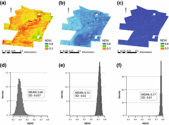
a–c RapidEye false-color subsets of field 100-01 (NIR-G-B); a 09-04-2011, wheat at tillering; b 28-06-2011, wheat at ripening; c 17-6-2010, canola at fruit development; d–f Histograms of NDVI of each subset raster, y-axes not graphically normalized due to value range of f to d and e

Classification of the averaged image
The NIR band of all remaining images was used to determine the final vegetation patterns, for the following two reasons:
-
(1)
NIR reflectance and yield relationship
Relative reflectance values in the NIR have been shown to quite adequately reveal patterns seen in yield maps. Reflectance in the NIR is an indicator of health for leaf tissue, cell structure and, therefore, the vitality of the plant (Gausman 1973, 1977; Jones and Vaughan 2010). Consequently, it is a major indicator for final yield. On a macro-scale, crops under advantageous growing conditions are more likely to grow taller and denser. They develop more biomass and leaves, which leads to increased NIR reflectance relative to the entire field. Leaf area index (LAI) is expected to be closely related to yield for certain crops, since grain yield is closely linked to crop growth (Serrano et al. 2000; Song et al. 2009). On the other hand, a reduction in LAI, similar to reduced chlorophyll content or surface temperature, is an expression of stress symptoms in plants (Baret et al. 2007). Reasons for stress symptoms are often water shortage, insufficient nutrient supply, and diseases like fungi or pests. Crops under stress often show decreased leaf area production and an increased senescence rate. On a micro-scale, the cell structure of the leaf is heavily altered, since the plant mobilizes all protein and minerals for the development of seeds. Senescence, either natural or stress-induced, is also accompanied by a decrease in leaf water content (Hurd-Karrer and Taylor 1929). This overall collapse of the leaf structure leads to decreased reflection in the NIR region, since the electromagnetic waves strongly scatter within healthy mesophyll tissue.
In conclusion, reflectance in the NIR is a very suitable indicator for field growing conditions and prospective yield. Naturally, the red-edge band as a chlorophyll indicator (Barnes et al. 2000) was also considered. However, empirical analysis of the data sets in this study did not show a strong correlation between reflection and yield as in the NIR band. Additionally, yield prediction on the basis of red-edge reflectance seems to be highly dependent on the phenological stage (He Ke-xun et al. 2013). In this study, the NIR reflectance values were converted into relative values, enhancing crop type and possibly regional independence.
-
(2)
Difficulties using vegetation indices for segmentation
The classification was not conducted using ratio images, such as NDVI, due to increased noise patterns and artefacts which are a common disadvantage of band ratios (Lillesand and Kiefer 1987). This effect is less desirable when a high degree of internal homogeneity is required for segmentation. The algorithm was nevertheless also tested by using NDVI images instead of NIR images. The results here were characterized by described noise patterns and numerous artefacts and did not lead to the same homogenous spatial patterns as when NIR is used.
Although precautions (single band basis, median filter) are taken to avoid small polygons in the end result, small features will still occur (< 3%). In agricultural practice, the user must decide how much detail is necessary and which features should be neglected.
Every NIR raster was normalized to a percentage, where 100% is equal to the average NIR value of each raster. To balance years with differing amounts of available satellite raster images, all rasters for each year were averaged (e.g. three rasters of 2009 become one average NIR raster). The resulting yearly average raster were also normalized. The subsequent raster was processed using a 7 × 7 median filter for six times to smooth boundaries and eliminate small fragments. Of course, the use of such intense smoothing filters had a strong impact on the level of detail and information in the image. However, the focus here was on the delineation of geometric zones. In precision agriculture applications, spatial zones do not necessarily benefit from small-scale details, since farming machinery has practical limits when it comes to fine-tuned control and implementation of highly-detailed GIS data.
The post-filter raster was classified into five value ranges, using quantiles of 10, 35, 65 and 90%. Due to the fact that every averaged NIR subset may have different value ranges, predefined values for separate classes are not feasible. The quantile values were chosen empirically on field 100-01 and others. The goal was to achieve class boundaries that generate well-balanced (amount of pixel) and clearly visual spatial classes. A change of the quantile values may lead, e.g. to a dominant ‘middle’ class and very marginal classes of very low and very high NIR values.
A cluster method (e.g. k-means) was not used at this point, because the generated clusters a) were not guaranteed to entail an “average” class with values around 100% NIR reflectance, b) lack of information about their relative sorting (“very low” to “very high” and c) therefore lack of a stable, re-occurring control factor like the preset quantile thresholds.
In the process of (visually) analyzing the yield maps and satellite images of field 100-01 and neighboring fields, the class number of five was found to be suitable to map and reflect the heterogeneity of especially large fields. The odd number ensures a resulting “average” middle class. In theory, every desirable class number can be accomplished by the algorithm. Less classes (3) could be considered for a broader overview or in the case of low-contrast patterns. More classes (7) would lead to a more fragmented result, which would be less feasible for technical implementation into current machine systems for fertilizer or seed distribution. These systems mostly work in increments (e.g. ± 20% grain), rather than with continuous rates, which justifies the decision on discrete classes. An odd number of classes is required to generate an average class.
Every class was exported into a polygon (not necessarily continuous), with which further analysis could be done. The resulting classes resembled zones of increasing vitality, relative to one another, which is why the five classes were named “very low” (1), “low” (2), “average” (3), “high” (4), “very high” (5) yield expectation.
Attributes of classes
To better assess the vitality status and yield expectancy of each class, and because the value range of the reflection within the NIR band seemed quite narrow, every class was additionally assigned a relative NDVI value and stored in a protocol. This value was generated by averaging all disturbance-free NDVI rasters with a NDVI between 0.3 and 0.78. For every class, the mean NDVI value within the class polygon was extracted, resulting in five relative NDVI values in percent. In this study, these NDVI values were highly linear (R2 > 0.9) to the relative yield values extracted from an interpolated yield map (average of multiple years, corresponding to satellite data selection). Since no universal, field-independent conversion equation from relative NDVI to relative yield could be determined, the results shown in this paper will refrain from focusing on these NDVI values.
Validation with yield data
The segmentation algorithm aims to give insights into yield distribution, especially for farmers lacking sufficient or total yield maps of their fields. In order to test the segmentation result in regard to yield expectancy zones, actual yield data were used for this validation (described in “Farm data”).
Stratified sampling
For validation, the concept of stratified sampling was preferred. As described in Webster and Oliver (1990), the sample points for validation were randomly distributed within regular grid cells, dividing the target raster area. Sample points within a 10 m buffer of the segmentation boundaries were eliminated. The sample size ranged around roughly 6%.
Yield values are based on point measurements, converted into relative values in % and averaged over the selected years. For each sample point, the relative yield value and the corresponding class id (1–5) were extracted.
The result was plotted as a boxplot, depicting relation and separability between each class. In addition, two statistical tests were applied: (a) the Kruskal–Wallis Test and (b) the Pairwise T Test (class ID versus relative yield value). The result with a p-value < 2.2e−16 confirmed the general separability of the five classes, even if run based on different sample points.
The pairwise T-Test applied compares each test series with one another and tests if there are statistically significant differences. This test normally requires normally distributed data, which is not necessarily given in this case. However, this condition may be violated if the number of sample points is high (Bartlett 1935) and the variance of the test series is comparable. With both of these being the case, the test was run a second time with logarithmic transformed values, to assure normality and test the validity. Additionally, the Pairwise Wilcox-Test for data without a normal distribution was run.
Results and discussion
After the automatic selection process, 14 out of 74 rasters for field 100-01 remained for segmentation (Table 2). Data from the years 2012 and 2013 were neglected by the algorithm, which will be examined later on. Therefore, the method is discussed based on a result from five non-continuous years (Table 2).
Figure 4 shows a final result of the segmentation process, compared to the averaged relative yield map of the corresponding years (2009, 2010, 2011, 2014, 2015). On first examination, the five classes resembling yield expectation zones (YEZ) moderately resemble the actual yield zones of high-, low- and medium yield.

Left: left Segmentation result; middle: relative yield map; right: histogram of yield raster. Average of years: 2009, 2010, 2011, 2014, 2015
Validation
All three statistical tests had p-values lower than the significance level (0.05), indicating a good separability of the five determined classes (Table 3).
Despite that, the boxplot (Fig. 5) still shows overlapping sampling values for every segment, whereas only segment 1, “very low yield expectancy”, appears to have slightly more discrete values than the other segments. Statistically, the Pairwise T-Test indicates independence between the classes.

Boxplot of sampling result, yield per segment
This overlapping of classes and left-skewed outliers is apparent in all segmentation test runs, even if the criteria (quantiles of class boundary; number of classes; NDVI thresholds as described above) for segment building are adjusted. Due to the overall high yield potential of field 100-01 (and therefore lack of strong contrast), the segmentation process has difficulties in distinguishing five apparently separated classes. An average yield map of the years 2009, 2010, 2011, 2014, 2015 does not present drastic yield variance over the field (Fig. 4), compared to fields in more vulnerable regions of Germany (Dobers 2005). The relative yield ranged from 25.0 to 141.9% (mean: 102.2, SD: 8.5%), whereas field 100-01 yields were above average and could be assumed to be relatively homogenous with a small yield variance.
Interpretation of results
NDVI and yield expectation relationship
The result shows the capacity of the method to form zones of different growth and yield levels for one field. However, it is problematic to reliably link these zones to percent-based relative yield values, and even more difficult to determine absolute yield values. A comparison of the five NDVI mean values with the actual yield values (mean value per class) reveals a highly linear relationship (R2 = 0.97), as well as NDVI values that are slightly lower (1–2%) than the mean relative yield values per class. Unfortunately, any empirical relationship determined for this field cannot be applied elsewhere, since a universal conversion from vegetation indices to yield values does not exist. Numerous efforts have been made to determine this relationship (Shanahan et al. 2001; Doraiswamy et al. 2003; Dalla Marta et al. 2013), with results indicating that replicability is mostly limited by crop type and climate zone. In this study, however, the focus is on identifying field zones of similar crop growth and vitality, regardless of the crop type cultivated. Therefore, the resulting crop patterns resemble a mixed signal of vitality patterns indicated by more than one crop type or even crop group. For absolute yield estimation, crop type knowledge as well as date and duration of critical phenological stages (Idso et al. 1980) are required in order to use the given satellite data and spectrally sensitive parameters impacting yield (Dalla Marta et al. 2013). This algorithm, however, seeks simplicity and functionality based on multispectral satellite images alone.
Disregard of crop type
The individual demands and phenological characteristics of crop types has not yet been considered by the algorithm. It can be argued that each crop type responds differently to field inventory and development prerequisites, and should therefore not be compared to other crop types. However, the analysis of satellite images, yield maps, soil and nutrient data of field 100-01 and the rest of the farm shows that the main drivers for re-occurring crop patterns are soil type and nutrient supply (Fig. 10). This observation is relevant for the crop types grown in the area: cereal, canola, maize and sugar beet. Vitality patterns are stronger in more sensitive crop types such as cereal, and more prominent under unfavorable weather conditions. Still, for the image segmentation, the crop cultivated is of no importance. The thresholds only select subsets with a certain amount of spectral heterogeneity. In most cases—at least during early phenological stages or at the transition between green and dry biomass—the plants reveal spatial patterns regardless of the type.
The algorithm currently yields good results even without the crop information, and can be validated even if the result shows a mixed crop signal. With an increasing number of satellite images and recorded years, the impact of specific phenological events, crop type specifications, or outstanding weather conditions would be alleviated However, it is equally true that the algorithm could be even better with knowledge of the crop type. Hence, future research could focus on adapting the algorithm to crop families (e.g. cereal; discussed further in the section “Outlook and Possibilities”).
Stability of the results
-
(1)
Variation of input years
Figure 6 shows the segmentation and validation results of three trial runs with different input years. Figure 6a is the result of the fully automated selection, which includes data from years 2009 to 2011 and 2014 to 2015. The result is similar to that of 2009–2011 (Fig. 6c). Figure 6b lacks year 2009, and appears to produce a much more homogenous result. The classes appear to be the most separable in Fig. 6c, the only test run without the year 2015. For this year, the yield data were only moderately reliable due to technical difficulties during harvest.

a–c Segmentation results of different test runs; a automatic selection (years 2009, 2010, 2011, 2014, 2015); b years 2010, 2011, 2014, 2015; c period of 2009–2011; d–f corresponding average yield maps; g–i Boxplots of sampling, yield per class; j–l histograms of average NIR raster, on which basis classification is done
It is clear that the segmentation results can differ depending on the selected satellite imagery. This is why the target parameter is yield expectancy and not yield potential. Additionally, the result has to be interpreted as average yield expectancy for the n number of years (which are selected for segmentation) under the conditions x (weather and growing conditions), which were present in the selected years. Consequently, the segmentation result is a reflection of spatial growth and vitality variability over plot 100-01.
Data from the year 2012 was not selected due to field partitioning in this year (wheat/sugar beet). For 2013 (wheat), an insufficient number of cloud-free images were available and the remaining images did not match the thresholds.
The year 2009 had an obvious impact on segment building, which is explained by the combination of crop type and nutrient supply. The rectangular patch of low yield expectancy in the NW corner of field 100-01 is lacking in several nutrients (Fig. 10), primarily indicated by wheat, as is the case in 2009 and in 2011 (Figs. 7, 10). If 2009 is not taken into account, the image changed (Fig. 6b) to a more homogenous result, showing less high-contrast nutrient patterns and more closely resembling soil type and relief patterns (Fig. 10).This change is explained by the dynamics of field 100-01. For one, the farmer was able to compensate the nutrient deficiencies from 2009 onwards (Fig. 10). Additionally, his precision farming management led to an increasing equalization of yields, represented in Fig. 8 by the decreasing value ranges in boxplots of 2009, 2011 and 2013 (all wheat).

Segmentation run on satellite data for each year, 2010 and 2015 are only based on one input image. The “mean result” is—as the automatic segmentation—based on all the displayed years

Upper row: validation boxplots; segments (2009–2011) versus average yield in % of single year yield maps; lower row: yield maps of years 2009–2015 (wheat, canola, wheat, wheat, canola, wheat); map 2009 includes data gaps; map 2015 is a little unreliable, due to technical problems during harvest, resulting in gaps in yield
This successful development in farming practice has the disadvantage of affecting the stability and reliability of this segmentation algorithm, when there are simply no high-contrast plant patterns on a field. The NIR image can still be classified by quantiles, but the resulting classes can no longer be successfully validated for their separability (Fig. 8). The value ranges of each class are very similar, and small segments with a low pixel count (e.g. class number 5) do not fit yield maps. This phenomenon is reflected in the histogram of the averaged NIR band subset (Fig. 6k), which is slightly less stretched than the other histograms. It can be concluded that the segmentation results following averaged NIR subset histograms with low scatter of values and high unimodality are not trustworthy. Classes with a very low number of pixels should also be evaluated with caution since they mostly do not coincide with the yield data.
For dynamic fields like 100-01, five or more growing seasons are required to depict average patterns and to compensate strong changes or high impacts of crop types and overall conditions. For other fields, a time frame of three years is enough to map out crop pattern.
-
(2)
Validation with single yield maps
In precision farming practice, the question arises as to the reliability of computed MZ, and whether they can be utilized for adapting management in future cultivation seasons. In principle, the presented segmentation algorithm can fulfil these requirements, if the crop patterns are more or less stable and high in contrast over multiple years. In the case study of field 100-01, this demand can only be met to a certain extent. Figure 8 shows the validation boxplots of the five segments (result of 2009–2011, Fig. 6c) versus the relative yield of single yield maps. Ideally, the order of the mean relative value continuously increases from segments 1 to 5. This is the case for the yield maps of 2009, 2011, 2013 and 2015—all of which were years of wheat cultivation. However, the range of yield values and the position of the boxes change. Despite yearly individual weather regimes, the strong crop patterns of 2009 and (partially) of 2011 decreased over time. This was due to the sustainable management of field 100-01 by the farmer, who constantly equalized nutrient deficiencies and optimized fertilization during the growing season. This explains why, in this case, the segmentation result is not always applicable for every year.
The greatest potential of the algorithm lies within fields where there is no comparable positive change, and crop patterns are more or less stable. Otherwise, the result has to be interpreted strictly as what it is: an averaged reflection of plant growth over multiple years. As Fig. 8 shows, the segmentation does not validate well with canola yield maps (2010, 2014). For a detailed analysis from a farmer’s perspective and the linked crop-type-specific measures, crop cycle information is needed.
However, the multi-year approach is still feasible because it does not favor crop specifications, but rather growth patterns with sufficient impact.
Method transferability to other fields
The automatic segmentation method was tested on three other farm fields, with varying areas and crop rotations (Table 4). Validation was likewise carried out with yield data (for the one season of sugar beet, yield data was not recorded).
The result (Fig. 9) shows the successful transferability of the method to other fields, which is attributable to the fact that all three plots show heterogeneous crop patterns for all years and are less dynamic than field 100-01. Test runs comparing the number of input years (3 vs. 6 years) resulted in similar results. The authors can therefore conclude that the algorithm performs well with a small amount of multi-temporal images (from 3 years)—if high contrast crop patterns predominate and if these are roughly spatially stable. This is mostly the case when crop patterns are mainly inherited by soil patterns, which is generally the case for these three fields (Fig. 9i). However, a large number of satellite images is still preferred, since the result is increasingly independent of crop type impact on patterns and temporal changes due to weather events.

a–c Segmentation result of field 200-01, 360-01, 270-01: 2009–2015; d–f validation boxplots; g–i soil map for each field
The size of a field does not matter. It can be up to the farmer in practice, as to whether five classes of yield expectancy are suitable for small fields like 270-01, or if three are sufficient.
Outlook and possibilities
Therefore, suggested future improvements include the implementation of a cloud mask and further testing of vegetation indices and existing studies for the derivation of yield values. This testing would require knowledge of the crop type and could be addressed by either a crop classification method (Itzerott and Kaden 2006; Foerster et al. 2012) or better yet by manual input of the potential user. These users are assumed to be farmers and agricultural consultants, interested in cultivating their crop with precision farming methods.
The method offers a quick delineation of the desired field, especially if yield maps are not or are insufficiently available. The segmentation could then be used for management decisions in fertilization, seeding or crop protection.
An upcoming milestone will be the coupling of the segmentation results with additional geospatial data, such as soil, relief and nutrient maps. This would allow for further optimization of the results and enable a transition from yield expectancy zones to yield potential zones. Additionally, the fusion of different multispectral sensor systems such as RapidEye, Sentinel-2 and Landsat could be an attractive method for further exploiting the big data pool and increasing the density of information for image segmentation.
With a vast data base and additional crop information from the user, the segmentation could also be computed for crop types or families, adding more stability and knowledge for crop-specific strategies.
Conclusion
This study presented a straightforward algorithm for the delineation of crop patterns on agricultural fields based solely on optical multispectral satellite data, but with certain limitations. The crop patterns can be interpreted as relative yield expectancy zones, and are influenced by prior growing conditions on a field. The result can be utilized as potential MZ, in order to implement and enhance precision farming practices. The algorithm operates with atmospherically-corrected remote sensing reflectance data, and does not need any further information besides the field outlines. Consequently, the method enables an effortless and quick overview of past averaged growing conditions, without manual work. As such, this algorithm addresses upcoming important developments of big data, open source satellite data access and digital/smart farming.
As a disadvantage, the method is unable to use partly cloud-covered images and suffers slightly from images with a strong tramline imprint, leading to noisy images which require smoothing filters. The result is also unreliable for fields lacking crop patterns and homogenous growing conditions, which is indicated by the output variables of the algorithm. As with numerous agricultural remote sensing methods, parameters and values are derived from image interpretation. Although the segmentation result could be validated with yield maps, it is also an interpretation of crop spectral characteristics. The gross division of crop patterns can be assumed to reflect overall growing conditions. However, small adjustments of the algorithm’s parameters are reflected in changes on a pixel scale, confirming the belief that actual crop can seldom be addressed by image interpretation on a detailed scale. Generally, algorithms based on optical remote sensing are always dependent on the availability of sensor data for the desired time frame and the quality of the data.
References
Ahamed, T., Tian, L., Zhang, Y., & Ting, K. C. (2011). A review of remote sensing methods for biomass feedstock production. Biomass and Bioenergy, 35(7), 2455–2469. https://doi.org/10.1016/j.biombioe.2011.02.028.
Ahn, C.-W., Baumgardner, M. F., & Biehl, L. L. (1999). Delineation of soil variability using geostatistics and fuzzy clustering analyses of hyperspectral data. Soil Science Society of America Journal, 63(1), 142. https://doi.org/10.2136/sssaj1999.03615995006300010021x.
Amt für Geoinformation Vermessungs- und Katasterwesen (Office for geoinformation, survey and land registry). (2011). DGM 5—Digitales Geländemodell Gitterweite 5 m (digital elevation model grid 5 m). Schwerin, Mecklenburg-Vorpommern, Germany. https://www.laiv-mv.de/Geoinformation/Geobasisdaten/Gelaendemodelle/.
Atzberger, C. (2013). Advances in remote sensing of agriculture: Context description, existing operational monitoring systems and major information needs. Remote Sensing, 5(2), 949–981. https://doi.org/10.3390/rs5020949.
Baret, F., Houlès, V., & Guérif, M. (2007). Quantification of plant stress using remote sensing observations and crop models: The case of nitrogen management. Journal of Experimental Botany, 58(4), 869–880. https://doi.org/10.1093/jxb/erl231.
Barnes, E. M., Clarke, T. R., Richards, S. E., Colaizzi, P. D., Haberland, J., Kostrzewski, M., et al. (2000). Coincident detection of crop water stress, nitrogen status and canopy density using ground-based multispectral data. In Proceedings of the 5th International Conference on Precision Agriculture and Other Resource Management (pp. 15). Madison, WI, USA: American Society of Agronomy, Crop Science Society of America, Soil Science Society of America.
Barnes, E., Sudduth, K., Hummel, J., Lesch, S., Corwin, D., Yang, C., et al. (2003). Remote- and ground-based sensor techniques to map soil properties. Photogrammetric Engineering and Remote Sensing, 69(6), 619–630.
Bartlett, M. S. (1935). The effect of non-normality on the t distribution. Mathematical Proceedings of the Cambridge Philosophical Society, 31(2), 223. https://doi.org/10.1017/S0305004100013311.
Basnyat, P., McConkey, B., Selles, F., & Meinert, L. (2005). Effectiveness of using vegetation index to delineate zones of different soil and crop grain production characteristics. Canadian Journal of Soil Science, 85(2), 319–328.
Behling, R., Roessner, S., Segl, K., Kleinschmit, B., & Kaufmann, H. (2014). Robust automated image co-registration of optical multi-sensor time series data: database generation for multi-temporal landslide detection. Remote Sensing, 6(3), 2572–2600. https://doi.org/10.3390/rs6032572.
Blackmore, B. S., & Marshall, C. J. (1996). Yield mapping; errors and algorithms. In P. C. Robert, et al. (Eds.), Precision Agriculture: Proceedings of the 3rd International Conference (pp. 403–416). Madison, WI, USA: American Society of Agronomy, Crop Science Society of America, Soil Science Society of America (ACSESS publications). https://doi.org/10.2134/1996.precisionagproc3.c44.
Boydell, B., & McBratney, A. B. (1999). Identifying potential within-field management zones from cotton-yield estimates. Precision Agriculture, 3(1), 9–23. https://doi.org/10.1023/A:1013318002609.
Bundesanstalt für Geowissenschaften und Rohstoffe. (2006). Bodenübersichtskarte (Soil overview map) 1:200.000 (BÜK200)—CC2342 Stralsund. Hannover, Germany.
Cambouris, A. N., Nolin, M. C., Zebarth, B. J., & Laverdiere, M. R. (2006). Soil management zones delineated by electrical conductivity to characterize spatial and temporal variations in potato yield and in soil properties. American Journal of Potato Research, 83(5), 381–395.
Cohen, S., & Levi, O. (2013). Combining spectral and spatial information from aerial hyperspectral images for delineating homogenous management zones. Biosystems Engineering, 114(4), 435–443. https://doi.org/10.1016/j.biosystemseng.2012.09.003.
Dalla Marta, A., Grifoni, D., Mancini, M., Orlando, F., Guasconi, F., & Orlandini, S. (2013). Durum wheat in-field monitoring and early-yield prediction: Assessment of potential use of high resolution satellite imagery in a hilly area of Tuscany, Central Italy. The Journal of Agricultural Science, 153(1), 68–77. https://doi.org/10.1017/S0021859613000877.
De Benedetto, D., Castrignanò, A., Rinaldi, M., Ruggieri, S., Santoro, F., Figorito, B., et al. (2013). An approach for delineating homogeneous zones by using multi-sensor data. Geoderma, 199, 117–127. https://doi.org/10.1016/j.geoderma.2012.08.028.
Dobers, E. S. (2005). Verbesserung und Erweiterung digitaler Bodenkarten unter Verwendung des Transferable Belief Models (Using the Transferable Belief Model for the improvement and extension of digital soil maps). In DBG-Workshop: Methoden zur Datenaggregierung und –regionalisierung in der Bodenkunde, der Bodengeographie und in Nachbardisziplinen 2005. Jena, Germany.
Doerge, T. (1999). Yield map interpretation. Journal of Production Agriculture, 12(1), 54–61.
Doraiswamy, P. C., Moulin, S., Cook, P. W., & Stern, A. (2003). Crop yield assessment from remote sensing. Photogrammetric Engineering and Remote Sensing, 69(6), 665–674.
Foerster, S., Kaden, K., Foerster, M., & Itzerott, S. (2012). Crop type mapping using spectral–temporal profiles and phenological information. Computers and Electronics in Agriculture, 89, 30–40.
Franzen, D. W., Hopkins, D. H., Sweeney, M. D., Ulmer, M. K. M. K., & Halvorson, A. D. (2002). Evaluation of soil survey scale for zone development of site-specific nitrogen management. Agronomy Journal, 94(2), 381–389. https://doi.org/10.2134/agronj2002.0381.
Fridgen, J., Kitchen, N., Sudduth, K., Drummond, S., Wiebold, W., & Fraisse, C. (2003). Management Zone Analyst (MZA): Software for subfield management zone delineation. Agronomy Journal, 96(1), 100–108.
Fu, Q., Wang, Z., & Jiang, Q. (2010). Delineating soil nutrient management zones based on fuzzy clustering optimized by PSO. Mathematical and Computer Modelling, 51(11), 1299–1305. https://doi.org/10.1016/j.mcm.2009.10.034.
Gausman, H. W. (1973). Photomicrographic record of light reflected at 850 nanometers by cellular constituents of Zebrina Leaf Epidermis. Agronomy Journal, 65(3), 504. https://doi.org/10.2134/agronj1973.00021962006500030045x.
Gausman, H. W. (1977). Reflectance of leaf components. Remote Sensing of Environment, 6(1), 1–9. https://doi.org/10.1016/0034-4257(77)90015-3.
Ge, Y., Thomasson, J. A., & Sui, R. (2011). Remote sensing of soil properties in precision agriculture: A review. Frontiers of Earth Science, 5(3), 229–238. https://doi.org/10.1007/s11707-011-0175-0.
Haas, T. C. (1990). Kriging and automated variogram modeling within a moving window. Atmospheric Environment, 24(7), 1759–1769. https://doi.org/10.1016/0960-1686(90)90508-K.
Hank, T., Bach, H., & Mauser, W. (2015). Using a remote sensing-supported hydro-agroecological model for field-scale simulation of heterogeneous crop growth and yield: Application for wheat in Central Europe. Remote Sensing, 7(4), 3934–3965. https://doi.org/10.3390/rs70403934.
Hornung, A., Khosla, R., Reich, R., Inman, D., & Westfall, D. G. (2006). Comparison of site-specific management zones: Soil-color-based and yield-based. Agronomy Journal, 98(2), 407. https://doi.org/10.2134/agronj2005.0240.
Hurd-Karrer, A. M., & Taylor, J. W. (1929). The water content of wheat leaves at flowering time. Plant Physiology, 4(3), 393–397.
Idso, S. B., Pinter, P. J., Jackson, R. D., & Reginato, R. J. (1980). Estimation of grain yields by remote sensing of crop senescence rates. Remote Sensing of Environment, 9(1), 87–91. https://doi.org/10.1016/0034-4257(80)90049-8.
Itzerott, S., & Kaden, K. (2006). Ein neuer Algorithmus zur Klassifizierung landwirtschaftlicher Fruchtarten auf Basis spektraler Normkurven (A new algorithm for the classification of agricultural crop on the basis of spectral standard curves). Photogrammetrie, Fernerkundung, Geoinformation: PFG, 6, 509–518.
Jensen, J. R. (2007). Remote sensing of the environment: An earth resource perspective (2nd ed.). Upper Saddle River, NJ, USA: Pearson Prentice Hall.
Jones, H. G., & Vaughan, R. A. (2010). Remote sensing of vegetation. New York: Oxford University Press.
Ke-xun, He, Shu-he, Zaho, Jian-bin, Lai, Yun-xiao, Luo, & Zhi-hao, Qin. (2013). Effects of water stress on red-edge parameters and yield in wheat cropping. Spectroscopy and Spectral Analysis, 33(8), 2143–2147. https://doi.org/10.3964/j.issn.1000-0593(2013)08-2143-05.
Kitchen, N. R., Sudduth, K. A., Myers, D. B., Drummond, S. T., & Hong, S. Y. (2005). Delineating productivity zones on claypan soil fields using apparent soil electrical conductivity. Computers and Electronics in Agriculture, 46(1–3), 285–308. https://doi.org/10.1016/j.compag.2004.11.012.
Lark, R. M. (1998). Forming spatially coherent regions by classification of multi-variate data: An example from the analysis of maps of crop yield. International Journal of Geographical Information Science., 12(1), 83–98. https://doi.org/10.1080/136588198242021.
Lark, R. M., & Stafford, J. V. (1997). Classification as a first step in the interpretation of temporal and spatial variation of crop yield. Annals of Applied Biology, 130(1), 111–121. https://doi.org/10.1111/j.1744-7348.1997.tb05787.x.
Lillesand, T. M., & Kiefer, R. W. (1987). Remote sensing and image interpretation (2nd ed.). New York, USA: Wiley.
Lobell, D. B., Thau, D., Seifert, C., Engle, E., & Little, B. (2015). A scalable satellite-based crop yield mapper. Remote Sensing of Environment, 164, 324–333. https://doi.org/10.1016/j.rse.2015.04.021.
Lu, D. (2006). The potential and challenge of remote sensing-based biomass estimation. International Journal of Remote Sensing, 27(7), 1297–1328. https://doi.org/10.1080/01431160500486732.
Lück, E., Gebbers, R., Ruehlmann, J., & Spangenberg, U. (2009). Electrical conductivity mapping for precision farming. Near Surface Geophysics, 7(32), 15–25. https://doi.org/10.3997/1873-0604.2008031.
MacMillan, R. A., Pettapiece, W. W., Watson, L. D., & Goddard, T. W. (1999). A landform segmentation model for precision farming. In Robert P. C., Rust R. H., & Larson W. E. (Eds.), Precision Agriculture (pp. 1335–1346). Madison, WI, USA: American Society of Agronomy, Crop Science Society of America, Soil Science Society of America. https://doi.org/10.2134/1999.precisionagproc4.c36b.
Moran, M. S., Inoue, Y., & Barnes, E. M. (1997). Opportunities and limitations for image-based remote sensing in precision crop management. Remote Sensing of Environment, 61, 319–346.
Mulla, D. J. (2013). Twenty five years of remote sensing in precision agriculture: Key advances and remaining knowledge gaps. Biosystems Engineering, 114(4), 358–371. https://doi.org/10.1016/j.biosystemseng.2012.08.009.
Pedroso, M., Taylor, J., Tisseyre, B., Charnomordic, B., & Guillaume, S. (2010). A segmentation algorithm for the delineation of agricultural management zones. Computers and Electronics in Agriculture, 70(1), 199–208. https://doi.org/10.1016/j.compag.2009.10.007.
R Core Team. (2012). R: A language and environment for statistical computing. Vienna, Austria: R Foundation for Statistical Computing. Available at http://www.r-project.org/.
Rees, W. G. (2001). Physical principles of remote sensing. Cambridge, UK: Cambridge University Press.
Ren, J., Li, S., Chen, Z., Zhou, Q., & Tang, H. (2007). Regional yield prediction for winter wheat based on crop biomass estimation using multi-source data. In IEEE International Geoscience and Remote Sensing Symposium 2007 (pp 805–808). New York, USA.
Richter, R. (2010). Atmospheric/topographic correction for satellite imagery. ATCOR-2/3 users guide, version 7.1. Switzerland: ReSe Applications Schläpfer.
Sakamoto, T., Gitelson, A. A., & Arkebauer, T. J. (2013). MODIS-based corn grain yield estimation model incorporating crop phenology information. Remote Sensing of Environment, 131, 215–231. https://doi.org/10.1016/j.rse.2012.12.017.
Schepers, A. R., Shanahan, J. F., Liebig, M. A., Schepers, J. S., Johnson, S. H., & Jr Luchiari, A. (2004). Appropriateness of management zones for characterizing spatial variability of soil properties and irrigated corn yields across years. Agronomy Journal, 96(1), 195–203.
Seelan, S. K., Laguette, S., Casady, G. M., & Seielstad, G. A. (2003). Remote sensing applications for precision agriculture: A learning community approach. Remote Sensing of Environment, 88(1–2), 157–169. https://doi.org/10.1016/j.rse.2003.04.007.
Serrano, L., Filella, I., & Pen, J. (2000). Remote sensing of biomass and yield of winter wheat under different nitrogen supplies. Crop Science, 40, 723–731.
Shaddad, S. M., Madrau, S., Castrignanò, A., & Mouazen, A. M. (2016). Data fusion techniques for delineation of site-specific management zones in a field in UK. Precision Agriculture, 17(2), 200–217. https://doi.org/10.1007/s11119-015-9417-6.
Shanahan, J. F., Schepers, J. S., Francis, D. D., Varvel, G. E., Wilhelm, W. W., Tringe, J. M., et al. (2001). Use of remote-sensing imagery to estimate corn grain yield. Agronomy Journal, 93(3), 583. https://doi.org/10.2134/agronj2001.933583x.
Simbahan, G., Dobermann, A., & Ping, J. (2004). Site-specific management—Screening yield monitor data improves grain yield maps. Agronomy Journal, 96(4), 1091–1102.
Song, X., Wang, J., Huang, W., Liu, L., Yan, G., & Pu, R. (2009). The delineation of agricultural management zones with high resolution remotely sensed data. Precision Agriculture, 10(6), 471–487. https://doi.org/10.1007/s11119-009-9108-2.
Thenkabail, P. S. (2003). Biophysical and yield information for precision farming from near-real-time and historical Landsat TM images. International Journal of Remote Sensing, 24(14), 2879–2904. https://doi.org/10.1080/01431160710155974.
Tyc, G., Tulip, J., Schulten, D., Krischke, M., & Oxfort, M. (2005). The RapidEye mission design. Acta Astronautica, 56(1), 213–219. https://doi.org/10.1016/j.actaastro.2004.09.029.
Ustin, S. (Ed.). (2004). Manual of Remote Sensing, Volume 4, Remote Sensing for Natural Resource Management and Environmental Monitoring (3rd ed.). Hoboken, NJ, USA: Wiley.
van Alphen, B. J., Stoorvogel, J. J. 1999. A methodology to define management units in support of an integrated, model-based approach to precision agriculture. In: P. C. Robert, R. H. Rust, & W. E. Larson (Eds.), Precision Agriculture (pp. 1267–1278), Madison, WI, USA: American Society of Agronomy, Crop Science Society of America, Soil Science Society of America. https://doi.org/10.2134/1999.precisionagproc4.c30b.
Webster, R., & Oliver, M. A. (1990). Statistical methods in soil and land resource survey. New York, USA: Oxford University Press.
Whelan, B. M., McBratney, A. B., & Minasny, B. (1996). Spatial prediction for precision agriculture. In Robert, P. C., Rust, R. H., Larson, W. E. (Eds.), Proceedings of the 3rd International Conference on Precision Agriculture 1996 (pp. 331–342). Madison, WI, USA: American Society of Agronomy, Crop Science Society of America, Soil Science Society of America.
Yao, R.-J., Yang, J.-S., Zhang, T.-J., Gao, P., Wang, X.-P., Hong, L.-Z., et al. (2014). Determination of site-specific management zones using soil physico-chemical properties and crop yields in coastal reclaimed farmland. Geoderma, 232–234, 381–393. https://doi.org/10.1016/j.geoderma.2014.06.006.
Acknowledgements
The authors would like to thank Climate-KIC for project funding, Edgar Zabel and the cooperating farm for data and support. Further, we would like to thank Katharina Heupel (GFZ) for programming support and Eike Stefan Dobers (Applied University of Neubrandenburg) for support on content and agricultural knowledge. We thank the German Aerospace Centre (DLR) for providing the data from the RapidEye Science Archive (RESA 617 FKZ).
Author information
Authors and Affiliations
Corresponding author
Appendix
Appendix

Left: RapidEye subset, false-color (NIR-G-B), 14-05-2012 wheat and bare soil; right: NDVI histogram of field raster with strong bimodality, which would not pass the selection process of the algorithm

a Segmentation for single years, no suitable images in 2012–2013; b precipitation and temperature 2009–2015, weather station Greifswald by Deutscher Wetterdienst “German Weather Service”; c interpolated nutrient data of field 100-01(potassium, magnesium, pH and phosphorus), August 2010; d soil map of field 100-01 e relief of field 100-01
Rights and permissions
Open Access This article is distributed under the terms of the Creative Commons Attribution 4.0 International License (http://creativecommons.org/licenses/by/4.0/), which permits unrestricted use, distribution, and reproduction in any medium, provided you give appropriate credit to the original author(s) and the source, provide a link to the Creative Commons license, and indicate if changes were made.
About this article

Cite this article
Georgi, C., Spengler, D., Itzerott, S. et al. Automatic delineation algorithm for site-specific management zones based on satellite remote sensing data. Precision Agric 19, 684–707 (2018). https://doi.org/10.1007/s11119-017-9549-y
Published:
Issue Date:
DOI: https://doi.org/10.1007/s11119-017-9549-y