Estimation of horizontal and vertical translations of large images based on columns and rows mean energy matching

Abstract

In this paper mean energy lateral histograms have been developed and used for the translation of frames detection and for the estimation of a shift vector in large image frames. 2-D translation problem is solved by two almost independent 1-D problems based on the mean energy lateral histograms. We formulate a simple optimization for estimating vertical or horizontal translations of the frame. The optimization goal is to find the best match between energies (squared norms) of rows (columns) of the image and the reference frame. The shift estimate is calculated as the minimizer of the least squares, maximum deviation or the sum of absolute deviations criterion. However, the first criterion is preferred, the last two almost always gave the same results when the noise level is low. The proposed method is faster than the FFT based phase–correlation approach. An iterative version of the algorithm is presented which is very reliable and usually converges in at most two iterations. A randomized version of the method which reduce further the computational cost for large images problems is also proposed. Experimental results are provided and discussed.

1 Introduction

A gray-scale image may be treated as an $m \times n$ matrix of pixels, which means that it consists of $m$ rows and $n$ columns. At present, images typically have 5–10 mega pixels and image processing tasks are often optimization problems of this order of dimension. However, many image processing techniques involve treating the image as a two-dimensional signal (Lim 1990) or as 2$-$D objects.

The image (video stream) representation depends strongly among other things on geometric transformations in spatial image space (Hoggar 2006; Velten and Kummert 2006)—translation, rotation, enlargement; and transformations in pixel function space, such as color or/and intensity corrections. Especially affine transformations are observed in image registration, image reconstruction, image recognition, motion detection, shape and deformation measurements and many others (Alliney 1993; Brunelli 2009; Malepati 2010; Jähne 2005; Park et al. 2003; Pratt 2001; Stone et al. 2001; Sutton et al. 2009).

Horizontal and vertical shifts estimation is a common problem in image stabilization, i.e., the process of removing effects of unwanted camera movements from the captured images (video) sequence. Digital image stabilization is the algorithmic process of removing such undesired translation and/or rotation effects present in the captured image sequence. We want to generate a compensated image sequence using digital image processing techniques without mechanical devices such as gyro sensors (Malepati 2010). Many image registration algorithms are related to the stabilization of image sequences, since it frequently occurs that a sequence of images is corrupted by movements of the camera and the scene (Alliney et al. 1996).

Thus, the digital image stabilization algorithm compensates these undesired effects by performing translations (both vertically and horizontally) or rotations of the main part of the image and stabilizing the current position of image objects. Rotation and translation forms affine image transformation which retain spatial inter-pixel relations.

Various techniques have been proposed for image shift detection. Spatial-temporal approaches include block matching techniques (Brunelli 2009; Goobic et al. 2005; Liu and Zaccarin 1993; Malepati 2010; Rehan and Watheq 2006) direct optical flow estimation (Chang et al. 2002; Gilbert and Johnson 2002; Sutton et al. 2009), bit-plane matching (Ko et al. 1999), feature tracking (Censi et al. 1999) among others.

The other possibility is a method based on translational motion estimation (Stiller and Konrad 1999). In general, motion estimation is based on several local motion vectors from sub-images in different positions of the frame using some kind of block matching algorithm. The image stabilization system determines the global motion of a frame by processing these local motion vectors, and decides whether the motion of a frame is caused by undesirable fluctuation and should be corrected.

Often the motion prediction with a Kalman filter can be used for smoothing the motion parameters to reduce the motion noises. A Kalman filter removes short-term image fluctuations with retained smooth gross movements (Chang and Lai 2006; Erturk 2003).

There are many possible choices for the similarity (dissimilarity) function for block template matching techniques. Normalized cross-correlation is one of the methods used for template matching, a process used for finding incidences of a pattern or object within an image. In translated images fitting, both a registered image and a template (a reference frame) are the same or similar size. In such a case normalized cross-correlation or cosine similarity (cross-correlation without pixel function centering) is often used in a frequency-domain. Phase correlation uses the FFT approach to estimate the relative translative offset between two similar images (Brunelli 2009; Reddy and Chatterji 1996). The method can be efficiently applied for large frame translations. Unfortunately, it can be easily applied for cyclic-translations only. Otherwise, some kind of Gibbs effect can be observed. Furthermore, ideally bandlimited images do not exist in practice and several enhancement techniques have to be used (see for example Altmann and Reitbock 1984; Pratt 2001; Stone et al. 2001). Moreover, for non-integer shifts inverse transforming the phase correlation matrix would yield a discrete Dirichlet function, that has many additional peaks, instead of a single impulse (Balci and Foroosh 2006).

The computational complexity of FFT and IFFT computations (Brunelli 2009; Bouguezal et al. 1999; Lewis 1995) is $30 n^2 \log _{2} n$ for images consisting of $n \times n$ pixels. In comparison, costs of strict cross-correlation computations are $O(n^4)$.

Line Radon transform is another method which can be used for image translation detection (Milanfar 1999; Robinson and Milanfar 2003). It consists of projection and integration of image function (illumination or gray scale intensity) along the line at a given angle. It is known that translational motion in the image domain results in translational motion in the projection domain, so the motion analysis is made in the transform domain. It should be noted that projections at angles $0^{\circ }$ and $90^{\circ }$ can be obtained by summing pixels along columns and along rows of the image respectively (Robinson and Milanfar 2003).

The similar method of projecting is proposed by Davies under the name of the lateral histogram technique (integral lateral histogram) (Davies 1985, 2008). Alliney and Morandi (1986), Alliney et al. (1996) and Sibiryakov (2007) have used horizontal and vertical projections (laterals histograms) and one-dimensional FFT for determination of the displacement of each image in the sequence with respect to the one chosen as a reference.

In the paper (Cain et al. 2001) the lateral histograms are analyzed in the space-domain using vertical and horizontal non-normalized cross-correlation functions.

We restrict our attention to the problem of 2-D translations. In many optical applications it is the main problem of image registration. Translations are rather small, but a large accuracy is desirable (Chen et al. 2009; Chen and Yap 2008; Goobic et al. 2005; Guizar-Sicairos et al. 2008; Foroosh et al. 2002; Karybali et al. 2008; Ren et al. 2010; Sibiryakov 2007; Sibiryakov and Bober 2006; Tejada et al. 2011). The method developed here is based on similar to the integral lateral histogram technique (Davies 2005) or a mentioned projection method (Alliney and Morandi 1986). It generalizes the method presented in Skubalska-Rafajlowicz (2011). In our approach we compute the energy of rows and columns by adding squared pixels values along rows and columns instead of the strict addition of pixel values. The energy matching is closely related to normalized cross-correlation and can be used in an iterative manner leading to precise solutions even when translations in both directions are relatively large. Furthermore, the method is often more sensitive to small shifts than the same method based on integral lateral histograms. We restrict our attention to integer (in pixels) translations thereby avoiding interpolation problems. These interpolation problems, however, can be solved independently assuming polynomial (or spline) representation of an image, but this outside the scope of this paper. The proposed method can be used as the first stage for a sub-pixel accuracy image registration, since in many such methods it is assumed that the integer shift has been (or can be) estimated by some other means (Stone et al. 1999, 2001). We also propose a randomized version of the algorithm that essentially samples the image’s columns (rows) for energy of the rows (columns) estimation and therefore reduces the computational burden introduced by large images. We assume, that a randomized algorithm is equipped with a random number generator producing a sequence of independent, uniformly distributed numbers indicated which columns and rows of the image under consideration should be chosen as a random representation of this image. Theoretical bounds on the number of elements used for energy estimation is similar to that obtained for random projections (Skubalska-Rafajlowicz 2011), but the method is about $n$ times faster than the previous one.

The rest of the paper is organized as follows: Sect. 2 defines the problem of fast similarity matching of image frames and templates using mean energy histograms. We propose here different criteria for comparison of mean energy projections of an image and a template. Computational costs of the method are analyzed. Section 3 outlines the iterative procedure for precise shift estimation and illustrates its very fast convergence. In Sect. 4 we discuss robustness of the method in the presence of an additive noise. To this end, we propose a randomized algorithm scheme in Sect. 5 which enables us to reduce the computational costs, especially in the case of large images. Section 6 provides simulations results performed both for mean energy lateral histograms and for internal lateral projections. Finally in Sect. 7 some concluding remarks are provided.

2 Detection of image translation

Let us assume that we have a reference frame $T=\{t(i,j)\}_{m,n}$, an image consisting of $m$ rows and $n$ columns, where $t(i,j) \in [0,1]$ is a pixel intensity in the location $(i,j)$.

The new image $F= \{f(i,j)\}_{m,n}$ is a part of a larger scene of the size $(m+2h \times n +2h)$, which can be used for the image stabilization, where $h$ is the maximal vertical and horizontal translation value measured in pixels. In the noiseless case we assume that there exist numbers $a,b \in [-h, -h+1, \ldots , 0, \ldots , h]$ such that $f(i-a,j-b)=t(i,j); \; i=1,\ldots ,m; \;j=1, \ldots , n$ or in a more general case, i.e., if we allow affine global changes of pixel intensity:

$$\begin{aligned} f(i-a,j-b)= \alpha t(i,j) + \beta ; \; i=1,\ldots ,m; \;j=1, \ldots , n. \end{aligned}$$

(1)

Different measures of similarity are used between the current frame and the template (Brunelli 2009). We can formulate the following normalized optimization problem.

Find $x,y \in [-h,h]$ such that

$$\begin{aligned} \min _{ x,y}P(x,y)=\min _{ x,y} \sum _{i=1}^{m} \sum _{j=1}^{n} \left( \frac{f(i-x,j-y)-\bar{f}(x,y)}{||f_{xy}-\bar{f}(x,y)||}-\frac{t(i,j)- \bar{t}}{||t- \bar{t}||} \right) ^2, \end{aligned}$$

(2)

where $\bar{f}(x,y)=\sum _{i=1}^{m} \sum _{j=1}^{n}f(i-x,j-y)/mn$,

$\bar{t}=\sum _{i=1}^{m} \sum _{j=1}^{n}t(i,j)/mn$ and

$$\begin{aligned} ||f_{xy}-\bar{f}(x,y)||=\sqrt{\sum _{i=1}^{m}\sum _{j=1}^{n} (f(i-x,j-y)-\bar{f}(x,y))^2} \end{aligned}$$

is the Frobenius norm of the centered (with respect to a mean pixel value) matrix $F$. Similarly, $||t- \bar{t}||$ is the Frobenius norm of the centered template $T$.

The goal function of the problem (2) equals to $0$, if $x=a$ and $y=b$. Simple reformulations of (2), i.e.,

$$\begin{aligned} P(x,y)&= \sum _{i=1}^{m} \sum _{j=1}^{n} \left( \left( \frac{f(i-x,j-y)-\bar{f}(x,y)}{||f_{xy}||}\right) ^2 +\left( \frac{t(i,j)- \bar{t}}{||t||}\right) ^2 \right) \nonumber \\&-2 \sum _{i=1}^{m} \sum _{j=1}^{n}\left( \frac{(f(i-x,j-y)-\bar{f}(x,y))(t(i,j)- \bar{t})}{||f_{xy}-\bar{f}(x,y)||\;||t- \bar{t}||}\right) \end{aligned}$$

(3)

lead to the well-known formula of the normalized cross-correlation (Brunelli 2009; Lewis 1995).

Thus, the problem of $C(x,y)$ maximization with respect to $x,y \in [-h,h]$, where

$$\begin{aligned} C(x,y)= \sum _{i=1}^{m} \sum _{j=1}^{n} \frac{\left( f(i-x,j-y)-\bar{f}(x,y))(t(i,j)- \bar{t}\right) }{||f_{xy}-\bar{f}(x,y)||\;||t -\bar{t}||}, \end{aligned}$$

(4)

which is the normalized cross-correlation formula (Brunelli 2009; Lewis 1995).

It is not exactly equivalent to (2), because it has the same optimal solution as the previous problems (2) and (3). The fact is elementary in image processing. One can check the claim just plugging-in adequate (i.e., with true shift values) images. If translations does not change the contents of the image, i.e., if $\bar{f}(x,y)=const$ for any $x$ and $y$, then we obtain $P(x,y)=2(1- C(x,y))$. Unfortunately, translations in the image coordinates introduce usually a part of new pixel values, thus this equivalence is only approximate. Cross correlation based methods are often preferred because they are more accurate (however slower) than the minimization of the sum of squared errors (2). Unfortunately, centering the pixel intensities with respect to their mean intensity value, i.e., the process of computing for every pixel its new value $(f(i-x,j-y)-\bar{f}(x,y)$, so that the new pixel intensity mean is zero after centering, is a rather time-consuming task (Lewis 1995). It can be avoided in phase-correlation based methods, but it happens on the costs of image windowing or filtration problems in frequency domain (see Hoggar 2006; Hoge 2003; Zhang et al. 2010 among many others).

2.1 Lateral mean energy histograms

Note, that one can also formulate alternative, simpler to compute, criteria functions which will attain their minima at the same values of $x=a$ and $y=b$. As a starting point we propose minimizing the goal function given by:

$$\begin{aligned} \sum _{i=1}^{m} \sum _{j=1}^{n} \left( \frac{f(i-x,j-y)-\bar{f}_{i-x.}}{||f_{r}||}-\frac{t(i,j)- \bar{t}_{i.}}{||t_{r}||}\right) ^2, \, \end{aligned}$$

(5)

where $\bar{f}_{i.}=\sum _{j=1}^{n} f(i-x,j-y)/n$ and similarly $\bar{t}_{i.}=\sum _{j=1}^{n} t(i,j)/n$ are the local means in the indicated rows $i.. ||f_{r}||$ and $||t_{r}||$ are the Frobenius norms of the matrices $\{f(i-x, j-y)-\bar{f}_{i-x.}\}_{mn}$ and $\{ t(i,j)- \bar{t}_{i.}\}_{mn}$, respectively.

A similar optimization problem can be stated by changing the order of summations and center within the image columns only.

$$\begin{aligned} \sum _{j=1}^{n} \sum _{i=1}^{m} \left( \frac{f(i-x,j-y)-\bar{f}_{.j-y}}{||f_{c}||}-\frac{t(i,j)- \bar{t}_{.j}}{||t_{c}||}\right) ^2, \, \end{aligned}$$

(6)

where $\bar{f}_{.j}=\sum _{i=1}^{m} f(i-x,j-y)/m$, similarly $\bar{t}_{.j}=\sum _{i=1}^{m} t(i,j)/m$ are the local means in the indicated columns $.j$. $||f_{c}||$ and $||t_{c}||$ are the Frobenius norms of the matrices $\{f(i-x,j-y)-\bar{f}_{.j-y}\}_{mn}$ and $\{ t(i,j)- \bar{t}_{.j}\}_{mn}$, respectively.

In all the above-mentioned problems a criterion function summarizes squared errors between pixel intensities of the image and corresponding pixels of the template. Furthermore, centering of the pixel intensity is done locally, separately for each row and each column of the image. As a consequence, two independent copies of an image have to be created. One of them, for the results of centering along rows and the other, for the results of centering along columns. We will explain further why this method of centering is convenient and leads to savings of computational costs when normalizing of data is necessary. We recall, that pixel intensity centering is advisable if and only if an offset ($\beta \ne 0$) in the pixel function can be expected. Similarly, a normalization (dividing by the Frobenius norm of the image intensity matrix) is necessary task only if changes in the piksel intensity scale ($\alpha \ne 1$) may happen.

From the optimization point of view it is possible to solve problems (5) and (6) parallely in an iterative and alternate manner, i.e., by optimizing successively in one direction at a time. Thus, we can solve problem (5) for vertical translation estimation and simultaneously problem (6) for horizontal translation estimation only. The optimization search can be performed in a form of successive or simultaneous iterations switched between vertical and horizontal search (usually referred to as Gauss–Seidel or Jacobi iterations). The first strategy means that a partial solution, a vertical translation estimate for example, is at once inserted into the horizontal optimization problem and so on. The Jacobi strategy seeks for vertical and horizontal translation estimates independently and after that adjusts both solutions.

It is assumed that during the one-dimensional optimization we have to match blocks consisting of image rows (columns) without changing pixels inside these blocks. In such a way, instead of pixel to pixel comparisons, it is faster to match some function values defined for image rows (columns).

Without loss of generality we can assume that each pixel value $x_{ij} \in [0,1]$. Let us define function $g(\mathbf x )=||\mathbf x ||_{p}^{p}$ which is relatively easy to compute and simultaneously can be used for distinguishing between vectors formed of an image rows (columns). If $g(\mathbf x )= ||\mathbf x ||_{1}$, i.e., we obtain (Alliney and Morandi 1986) vertical and horizontal projections obtained by summing pixels along columns and along rows of images respectively. Projections, in Davies’ terminology lateral histograms (Davies 2005), of an image are obtained by summing pixels along rows and along columns. Note, however, that a global centering is only allowed in this case, since centering in rows (columns) leads to a zero value in every centered sum along row (column).

In our approach $g(\mathbf x )=||\mathbf x ||_{2}^{2}$ is an energy of rows or columns, i.e., the function $g$ values are computed for every row and every column of the image under consideration and are obtained by adding squared pixel values (centered if necessary) along rows and columns, respectively.

Denote the mean energies of rows and columns of an image $X$ (centered if necessary) by

$$\begin{aligned} r_{i}(X)&= g(\mathbf x_{i.} )/n=\frac{1}{n} \sum _{j=1}^{n} x_{ij}^{2}, \; i=1, \ldots , m, \nonumber \\ c_{j}(X)&= g(\mathbf x_{.j} )/m=\frac{1}{m} \sum _{i=1}^{m} x_{ij}^{2}, \; j=1, \ldots , n, \end{aligned}$$

(7)

where $\mathbf x_{i.}$ and $\mathbf x_{.j}$ stand for $i$th row vector and $j$th column vector of image $X$, respectively. The factors $1/n$ and $1/m$ assert that $r_{i}(X), \;c_{j}(X) \le 1,$ $i=1, \ldots ,m$, $j=1,\ldots ,n$, $\; X \in [0,1]^{mn}$, where $X=F$ or $X=T$. So, after normalization we obtain the mean energy projection vectors in the following form:

$$\begin{aligned} \left\{ r_{i,norm}/n= \frac{ r_{i}(X)}{ n\sum _{i} r_{i}(X)} \right\} , \; \;\left\{ c_{j,norm}/m= \frac{ c_{j}(X)}{ m\sum _{j} c_{j}(X)} \right\} . \end{aligned}$$

(8)

One can verify that values of (8) do not dependent on $\alpha$ and $\beta$ (see (1) ) by substituting (1) and (7) into (8), where $\mathbf x_{i.}$ and $\mathbf x_{.j}$ stand for $i$-th centered row vector and $j$-th centered column vector, respectively. Row and column centering with respect to individual rows or columns means is performed in the same way as in (5) and (6).

Figure 1 shows non-normalized lateral energy histograms ($r_{i}$ and $c_{j}$) for a $2,300 \times 1,700$ image.

Fig. 1

Image ‘Grapes’ and its lateral energy histograms

2.2 Mean energy projections of image and template comparisons

Formally, there exist artificially constructed examples (e.g. chess board and its negative) such that two images have the same lateral histograms. Natural images are so rich in details that one can consider lateral histograms as their signatures.

We can formulate various simple criteria for comparisons of image $F$ histogram and a histogram of template $T$, instead of comparison of images pixel by pixel.

Note that the sequences $(r_{h+1}(T), \ldots , r_{m-h}(T))$ and $(c_{h+1}(T), \ldots , c_{n-h}(T))$, where $h >0$ is an integer denoting the maximal shift value, are similar to the parts of the lateral projections of the translated image $F$. So, these sequences should be matched with the mean energy lateral histograms $(r_{1}(F), \ldots , r_{m}(F))$ and $(c_{1}(F), \ldots , c_{n}(F))$ of image $F$. Alternatively, one can take the sequences $(r_{h+1}(f), \ldots , r_{m-h}(F))$ and $(c_{h+1}(F), \ldots , c_{n-h}(F))$ and look for the similar subsequences in histograms of template $T$, i.e., $(r_{1}(T), \ldots , r_{m}(T))$ and $(c_{1}(T), \ldots , c_{n}(T))$. This approach allows to reject new information introduced by a translated image. Thus, one may expect, that this method will be less robust to a translation in the other direction.

However, it should be indicated, that the method centering along rows and columns can be performed only once and does not need to be actualized. Furthermore, reorganization of adequate subsequences of lateral mean energy histograms can be performed very quickly using the partial sums of $r_{i}(F)$ and $c_{j}(F)$, respectively. For the sake of simplicity only, we will skip the normalization formulas in further considerations.

We propose here three different criteria for mean energy projections matching.

LS - least square error criteria

$$\begin{aligned}&\min \nolimits _{x } 1/(m-2h) \sum _{i=h+1}^{m-h} (c_{i-x}(F)-c_{i}(T))^2,\; x \in \{-h, \ldots , h\}, \nonumber \\&\min \nolimits _{y } 1/(n-2h) \sum _{j=h+1}^{n-h} (r_{j-y}(F)-r_{j}(T))^2,\; y \in \{-h, \ldots , h\}. \end{aligned}$$

(9)

Figure 2 shows LS values for vertical energy projections for image ‘Grapes’ and its copy translated by vector $(100,-1)$ (100 pixels horizontally to the right and $1$ pixel vertically down). Function (9) attains minimum for true vertical translation, i.e., $a=-1$, with minimum value equals to $0.519433$. The horizontal translation is the cause that this value is greater than $0$.

Fig. 2

LS criterion values for vertical shift estimation obtained for image ‘Grapes’ translated by vector $(100, -1)$

MAD - maximum of absolute deviation criteria

$$\begin{aligned}&min_{x } \max \nolimits _{i=h+1:m-h} |c_{i-x}(F)-c_{i}(T)|,\; x \in \{-h, \ldots , h\}, \nonumber \\&min_{y } \max \nolimits _{j=h+1:n-h} |r_{j-y}(F)-r_{j}(T)|,\; y \in \{-h, \ldots , h\}. \end{aligned}$$

(10)

Sum of absolute deviations criteria (SAD)

$$\begin{aligned}&min_{x } 1/(m-2h) \sum _{i=h+1}^{m-h} |c_{i-x}(F)-c_{i}(T)|,\; x \in \{-h, \ldots , h\}, \nonumber \\&min_{y } 1/(n-2h) \sum _{j=h+1}^{n-h} |r_{j-y}(F)-r_{j}(T)|,\; y \in \{-h, \ldots , h\}. \end{aligned}$$

(11)

2.3 Criteria analysis

Let ${\hat{a}}$ and $\hat{b}$ stand for estimated vertical and horizontal translations obtained by solving one of the optimization problems (9), (10) or (11). Note, that in the all cases the optimization process is very simple and independent from each other.

Figures 3 and 4 show values of criterion functions MAD, LS and SAD based on vertical energy (non-normalized) projections of template ‘Grapes’ and its copy translated by vector $(10,-10)$. Note that all the criteria indicate the true vertical shift ($a=-10$) in spite of the horizonal translation $10$. The formulas computed for normalized versions of images produce the same results (see Fig. 4 for comparisons).

Fig. 3

MAD (left panel) and SAD (right panel) criterion values for vertical shift estimation obtained for image ‘Grapes’ translated by vector $(10, -10)$

Fig. 4

LS criterion value for vertical shift estimation obtained for image ‘Grapes’ translated by vector $(10, -10)$ left panel—non-normalized data, right panel—normalized data

Nevertheless, the vertical translation estimate can be a little biased by the true horizontal shift and similarly, the horizontal translation estimate can be biased by the real vertical shift.

2.4 Errors introduced by orthogonal image translations

If vertical and horizontal translations are much smaller than dimensions $m,n$, their impact on mean energy values in columns and rows, respectively, is also small and an additive error can be bounded by $h/m$ or $h/n$, respectively. We recall that the pixel values are in $[0,1]$. The maximal difference in row (or column) energy introduced by replacing one pixel by another is $1^2=1$. So, replacing at most $h$ pixels by other pixels costs at most $h$ and a mean energy of given row (given column) changes at most by $h/m$ (or $h/n$).

Figure 5 presents vertical histograms (for non-normalized data) obtained for images ‘Grapes’ and its copy translated by vector $(-10,10)$. The histograms are almost the same, but a small translation between them can be observed.

Fig. 5

Vertical energy histogram obtained for images ‘Grapes’ and its copy translated by vector $(10, -10)$

3 Iterative procedure

Unfortunately, in general, the vertical translation estimate is biased by the true horizontal shift and simultaneously the horizontal translation estimate is biased by the real vertical shift.

An iterative procedure based on the successive, alternate estimation of a vertical and horizontal translation allows us to solve this problem. Of course, the consecutive iterations are possible, if one is able to obtain a new image corrected according to the last estimates. We prefer simultaneous corrections for both directions, because in most cases the precise estimate of a 2D shift was obtained at once (see Sect. 6).

Verification of the estimated shift. In the noiseless case criterions values close to zero indicate good position match. Nevertheless, it is advisable to perform a full matching formula for the core part of a template consisting of $m-2h$ central rows and $n-2h$ central columns and the best matched part of an image consisting of rows $h+1-{\hat{a}}, \ldots , m-h-{\hat{a}}$ and columns $h+1- \hat{b}, \ldots , n-h- \hat{b}$, i.e.,

$$\begin{aligned} V({\hat{a}}, \hat{b})=\frac{1}{(m-2h)(n-2h)} \sum _{i=h+1}^{m-h} \sum _{j=h+1}^{n-h}( t_{ij} -f_{i-{\hat{a}},j-\hat{b}})^2. \end{aligned}$$

(12)

In the case of an additive, independent with respect to an image and a template, Gaussian white noise with a covariance matrix $\sigma ^{2}I,\, V(a,b)/2$ estimates the noise variance $\sigma ^2$, so the variance of the observed noise should be taken into account in deciding about the acceptable error level $\epsilon$.

Algorithm To summarize, the algorithm for fast estimation of an image translation consists of the following steps.

• 1. (optional) Center rows and columns of image $F$ and template $T$.

• 2. Compute lateral mean energy histograms $\mathbf r$ and $\mathbf c$ according to (7).

• 3. (optional) Compute partial sums $pr(s)= \sum _{i=1}^{s} r_{i}, \;s=1,\ldots ,m$ and $pc(s)=\sum _{j=1}^{s} c_{j}, \;s=1,\ldots ,n$ and normalization factors for the template $(pr(m-h)-pr(h))^{-1}$ and $(pc(m-h)-pc(h))^{-1}$, respectively. Normalization factors for the image depend on $x$ or $y$ values and equal to $pr(m-h-x)-pr(h-x)$ or $pc(m-h-y)-pr(h-y)$, respectively.

• 4. Compute the values of the chosen criterion (9, 11 or 10) for vertical and horizontal histograms ($x=-h, -h+1, \dots , h$ or $y=-h, -h+1, \dots , h$, respectively). Optionally one can use normalizing factors according to:

  $$\begin{aligned} r_{i}(T)_{norm}&= \frac{r_{i}(T)}{pr(m-h)-pr(h)},\;i=h+1, \ldots , m-h,\\ r_{i-y}(F)_{norm}&= \frac{r_{i-y}(F)}{pr(m-h-y)-pr(h-y)},\;i=h+1, \ldots , m-h \end{aligned}$$

  for rows and according to

  $$\begin{aligned} c_{j}(T)_{norm}&= \frac{r_{j}(T)}{pc(m-h)-pc(h)},\;j=h+1, \ldots , m-h,\\ c_{j-x}(F)_{norm}&= \frac{c_{j-x}(F)}{pc(m-h-x)-pc(h-x)}, \;j=h+1, \ldots , m-h \end{aligned}$$

  for columns. This means, that instead of (9) the modified objective functions

  $$\begin{aligned}&\min _{x } 1/(m-2h) \sum _{i=h+1}^{m-h} (c_{i-x}(F)_{norm}-c_{i}(T)_{norm})^2,\; x \in \{-h, \ldots , h\},\\&\quad \min _{y } 1/(n-2h) \sum _{j=h+1}^{n-h} (r_{j-y}(F)_{{norm}}-r_{j}(T)_{norm})^2,\; y \in \{-h, \ldots , h\} \end{aligned}$$

  should be used. Similar changes should be done in formulas (11) and ( 10).

• 5. Find ${\hat{a}}$ which minimizes the chosen criterion for vertical mean energy histograms and find $\hat{b}$ which minimizes the chosen criterion for horizontal mean energy histograms.

• 6. If obtained optimization errors or value of (12) are not greater than the acceptable error level $\epsilon$, then STOP with ${\hat{a}}$ and $\hat{b}$ as the result. Otherwise, locate template in the position indicated by ${\hat{a}}$ and $\hat{b}$, adjust optimization limits, i.e., change from: $h+1$ and $m-h$ or $n-h$ (for rows and columns respectively) to $h+1+{\hat{a}}$ and $m-h +{\hat{a}}$ (or $n-h +\hat{b}$ and go to step $1$.

The algorithm can be used as direct non-recursive procedure. But, in some cases, iterative manner allows to reduce estimation errors. In such a case, iterate until convergence occurs, i.e., until optimization errors are smaller than $\epsilon$, or until (12) decreases. Other simple criteria combining vertical and horizontal matching errors, as for example, the sum of both of them, can be also applied.

The obtained solutions (estimated vertical and horizontal shifts) usually (for large images in low noise conditions) provide exact translations in one iteration. It can be verified in practice by checking the obtained criterion function values. If these values (for both directions) are close to zero (i.e., less than chosen level $\varepsilon$) then the algorithm stops. Otherwise we can repeat the algorithm starting from previously estimated positions. Formally, the algorithm stops when no improvement in criterion (12) is obtained. Monotonicity and boundedness from below of criterion values imply a convergence.

It should be indicated, the new iteration of the algorithm should start from recalculation of the image histograms. It can be done on the basis of reduced in the length (by translation of optimization limits) image rows and columns or adding additional new rows and columns from the image source. The last possibility means that the first iteration of the algorithm begins with $m \times n$ images taken from the center of larger images.

3.1 Computational complexity of the algorithm

The most expensive part of the algorithm is to compute energy histograms of an image and a template (see (7)). It consists of computing energy of each image pixel $x_{ij}^2 , \;i=1, \ldots , m \; j=1, \ldots , n$, i.e., it needs $m\,n$ multiplications. Computing both histograms costs $2\,m\,n$ additions.

Notice, that, if the algorithm is used for a sequence of images, the last image becomes a new template and its histograms are ready for use.

The optimization part of the algorithm is less costly. Namely, computing the chosen criterion value (9, 11 or 10) needs $3\,(n-2\,h)-1$ and $3\,(m-2\,h)-1$ elementary operations (addition, multiplications or comparisons) repeated $2\,h+1$ times. Summarizing, it is approximately $6\,(n+m)\,h$ elementary operations. Finding minimum among $2\,h+1$ values, when $h$ is small in comparison to $n$ and $m$, is negligible from the computational point of view.

Centering (along rows and columns separately) is performed twice with respect to all pixel values, so its computational complexity is $4\,n\,m$ per image. Thus, this procedure is more expensive than the process of computing energy histograms. Similarly as in spatial cross-correlation, it is not necessary, if no offset in pixel intensity is expected ( $\beta =0$ in (1)). Due this rather uncommon centering, the normalization of energy histograms (8) can be done relatively efficiently by using partial sums of appropriate histograms (see an optional part of Step 4). Namely, obtaining partial sums needs $n+m-2$ additions (Step 3). Further, the normalization is repeated $2\,h+2$ times, performing $2\,(m+n-4\,h)$ elementary operations. Summarizing, the normalization of histograms has $O(m+n)$ complexity. When $\alpha$ in (1) equals $1$, i.e., we do not expect changes in the pixel intensity scale, then the normalization should be avoided.

For comparison, $2$-D phase only correlation method has $O(n\,m (\log _{2}n + \log _{2}m))$ complexity with the implied constant depending on the method of counting operation in a complex domain (this constant equals $15$ if real operation are taken into account and complex operations are counted as adequately more costly than real, Brunelli 2009). This means that for $n=m=1,024$ we obtain $15\cdot 20\,n\,m$t. Notice, that we should add also the complexity of normalization and windowing. These costs are linear with respect to the number of image piksels $n\,m$.

Summarizing, the computational complexity of the proposed method is about $6\,n\,m+6\,(n+m)\,h$, assuming that the centering and normalization are avoided. Otherwise, one should add also $4\,n\,m$ and $4\,(h+1)\,(m+n)$. Thus, the ratio of the computational costs of our method to $2$-D phase only correlation method is equal to $0.036$ for $h=100$ and $n=m=1,024$.

4 Shift detection in the presence of an additive noise

The proposed methodology is robust to the moderate level of noise corrupting consecutive image frames. We assume that images are perturbed by a white Gaussian noise with a covariance matrix $\sigma ^2I$.

Theoretical analysis of behavior of formulas 9, 11 or 10 in the presence of noise is in general a very complicated task. Nevertheless, it is relatively easy to examine some crucial parts of these goal functions, namely the mean energy differences in the positions close to optimum. We restrict our attention to the energy of rows, because the energy of columns analysis is analogous. It is easy to see, that

$$\begin{aligned}&\Delta _{i}(F,T, noise)=r_{i}(F+ \varepsilon _{1})-r_{i}(T+ \varepsilon _{2})=r_{i}(F)-r_{i}(T) \nonumber \\&\quad +\frac{2}{n} \sum _{j=1}^{n}\left( f_{ij} \varepsilon _{1ij}-t_{ij} \varepsilon _{2ij} \right) + \frac{1}{n} \sum _{j=1}^{n} \left( \varepsilon _{1ij}^{2} -\varepsilon _{2ij}^{2} \right) . \end{aligned}$$

(13)

$\frac{1}{n} \sum _{j=1}^{n} \varepsilon _{1ij}^{2}$ and $\frac{1}{n} \sum _{j=1}^{n} \varepsilon _{2ij}^{2}$ follow $\sigma ^{2}/n \chi ^{2}_{n}$ distributions with the same means $\sigma ^{2}$ and the same variances $2 \sigma ^{4}$. Thus, the last summand in (13) is negligible, since the expectation of $\frac{1}{n}\sum _{j=1}^{n}(\varepsilon _{1ij}^{2}-\varepsilon _{2ij}^{2})$ equals zero and its variance is rather small for $\sigma ^{2}<1$. The second summand $\frac{2}{n} \sum _{j=1}^{n}(f_{ij}\varepsilon _{1ij}-t_{ij}\varepsilon _{2ij})$ follows the normal distribution $\mathcal N (0, \sigma \sqrt{2/n \sum _{i}(f_{ij}^2+t_{ij}^{2}})$, where $2/n \sum _{i}(f_{ij}^2+t_{ij}^{2} \le 4$.

Simplifying the analysis, we can assume that $\Delta _{i}(F,T, noise)=r_{i}(F)-r_{i}(T) + Z_{i}$, where each $Z_{i}$ is iid normal random variable with zero mean and the variance smaller than $4\sigma ^{2}$.

So, in the case of LS error function (9) for vertical direction, we have

$$\begin{aligned} E \left\{ 1/(m-2h) \sum _{i=h+1}^{m-h} \left[ \Delta _{i}(F,T, noise)^{2} - \left( r_{i}(F)-r_{i}(T)\right) ^{2} \right] \right\} \le 4\sigma ^{2}. \end{aligned}$$

(14)

The similar formula one can obtained for horizontal LS error function (9). The maximum absolute deviation objective (10) is non robust against noise.

5 Randomized algorithm

In the previous paper (Skubalska-Rafajlowicz 2011) we concentrate mostly on the problem of fast detection and estimation of translations in large image frames using random projections (Vempala 2004) which can be used for fast digital image stabilization, image registration etc. Recent results on random projections provide tools for dimensionality reduction, which retain (with prescribed accuracy and probability) the Euclidean norm of projected vectors and the Euclidean distances between pairs of these vectors. Random projection based image transformation is a linear projection from an image space to lower dimensional Euclidean space and may be treated as a kind of lossy compression (Jeong and Principe 2008; Tsagkatakis and Savakis 2009). However, the mentioned random projections have been found to be computationally efficient and sufficiently accurate when computationally time-consuming tasks are performed in an approximately isometrically equivalent Euclidean space (Skubalska-Rafajlowicz 2008), here we propose another method of defining a random projection based on uniform columns (rows) sub-sampling. Many randomized algorithms have been introduced for matrix approximation, matrix computation and image processing ( see for example Drinea et al. 2001; Woolfe et al. 2008; Xu et al. 1990, among many others). Uniform image columns and rows sampling during fast computing lateral energy projections $\mathbf r$ and $\mathbf c$ can be treated as a method of defining an approximate isometry with respect to row and columns vector norms. Instead of summing along all pixels in a row (in a column), we compute the mean energy of a row (a column) on the basis of randomly chosen pixels. Figure 6 shows horizontal mean energy projections for $100 \times 100$ image ‘Baboon’ obtained by summing along all rows and obtained by summing along uniformly sampled $50$ rows. Note, that a lateral histogram contains a lot of other information about the image structure. Here we can infer about the approximate column symmetry of ‘Baboon’.

Fig. 6

Horizontal mean energy projections for $100 \times 100$ image ‘Baboon’ obtained by summing along all rows and obtained by summing along uniformly sampled 50 rows

The method of randomization can be seen as sampling from a finite population. Let $Z$ be a discrete random variable which takes values from set $x_{1}^2, x_{2}^{2}, \ldots , x_{n}^{2}$ with equal probabilities $\frac{1}{n}$, where $x_{i} \in [0,1]$. Let $Z_{i}$ $i=1,\ldots , k$ be independent, identically distributed copies of $Z$. Using the well-known Hoeffding inequality (Hoeffding 1963) we obtain

$$\begin{aligned} \mathbf P \left\{ \left| \frac{1}{k} \sum _{i=1}^{k} Z_{i} -E[Z]\right| > \varepsilon \right\} \le 2 \exp { -2 \varepsilon ^{2}k}, \end{aligned}$$

(15)

where $E[Z]=\frac{1}{n} \sum _{i=1}^{n} x_{i}^{2}$. When $x_{i}^{2}$ stands for the energy of the $i$-th pixel in a row (alternatively column), then $E[Z]$ is the exact mean energy of that row (column) and $\frac{1}{k} \sum _{i=1}^{k} Z_{i}$ is its estimate. Let $\delta >0$ stands for an acceptable level of probability that the estimate differs from the true value $E[Z]$ by more than $\varepsilon >0$ for every row vector. Using the union bound we have

$$\begin{aligned} 2m \exp { -2 \varepsilon ^{2}k} \le \delta , \end{aligned}$$

(16)

Thus, we can expect that, if

$$\begin{aligned} k \ge \frac{\log 2m -\log \delta }{2\varepsilon ^{2}}, \end{aligned}$$

(17)

then with a probability of at least $1-\delta$ norms of any configuration of $m$ vectors will be approximated with $\varepsilon$ accuracy. Notice, that inequality (17) is formulated for $m$ rows of the image under consideration and subsampling is performed with respect to columns (we take $k$ from $n$ columns). If $\varepsilon$ is too small than it can happen that $k > n$. In such a case the required accuracy could not be guaranteed. Nevertheless, if the image is large, then the randomized algorithm allows us to obtain a good estimate of the mean energy histogram.

6 Experiments

In this section, we experimentally analyze the performance of the proposed method of image displacement estimation based on energy lateral histograms and compare it with the similar approach based on integral lateral histograms (Alliney and Morandi 1986; Davies 2005).

The images used for simulations are:

• 1. ‘Krill’ – Antarctic krill ommatidia.jpg ($1{,}158 \times 1{,}123$ pixels). Ommatidia of eye of Antarctic krill. We have used a gray level part of that image of the size $1{,}000 \times 1{,}000$ pixels, mean pixel intensity $0.235$ in $[0,\,1]$ scale.

• 2. ‘Grapes’ – image size $2{,}500 \times 1{,}700$ pixels, gray level scale, mean pixel intensity $0.45$ in $[0,\,1]$ scale (see Fig. 1).

• 3. ‘Polio’ – Polio EM PHIL 1875 lores.PNG. Electron micrograph of the poliovirus; image size $724 \times 1{,}000$ pixels ($700 \times 900$ pixels used), gray level scale, mean piksel intensity $0.584$ in $[0,\,1]$ scale.

• 4. ‘Struvite’ – Struvite crystals dog with scale 1.jpg, Struvite (magnesium ammonium phosphate) crystals found microscopically; image size $1{,}427 \times 1{,}175$ pixels ($1{,}000 \times 1{,}000$ pixels used), gray level scale, mean pixel intensity $0.847$ in $[0,\,1]$ scale.

• 5. ‘Baboon’ – image size $150 \times 150$ pixels ($100 \times 100$ pixels used), gray level scale, mean pixel intensity $0.503$ in $[0,\,1]$ scale (see Fig. 7).

  Fig. 7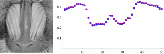

  

  $100 \times 100$ image ‘Baboon’ (left panel). Matching of horizontal energy histograms between ‘Baboon’ and its copy translated by (5, $-$5) pixels (right panel)

• 6. ‘Star1’ – artificial image of the size $1{,}050 \times 1{,}050$ piksels, the bright circle of radius $10$ px on dark ($0.3$) background.

• 7. ‘Star2’ – artificial image of the size $550 \times 550$ piksels, the bright circle of radius 10 px on dark ($0.3$) background.

• 8. ‘Uniform noise’ – artificial image of the size $1{,}050 \times 1{,}050$ piksels. Intensity image piksels were independently generated from the continuous uniform distribution on the unit interval $[0, 1]$. Five different images were generated.

In simulations translation values are chosen at random according to the discrete uniform distribution on $[-10,10]$, i.e., a replica of the image can be shifted at most by $(10, 10)$ or by $(-10,-10)$.

The operation of generating randomly shifted versions of the image was repeated 1,000 times for each test image (in the noiseless circumstances and with additive white Gaussian noise) and shift estimates are calculated by both the histogram-based methods that are used in combination with LS, SAD and MAD objective functions. The root mean square error (RMSE) was employed as a criterion for evaluating the accuracy of the image shift estimation in both directions.

6.1 Noiseless conditions

We have examined the performance of all version of the proposed algorithm for all combinations of possible integer shifts in both directions, taken from the interval $[-10,10]$. In noiseless case, the proposed method provides non erroneous shift estimates – one iteration was sufficient for all test images, except ‘Baboon’ image.

For ‘Baboon’ , when only one iteration of the algorithm has been performed, some estimation errors occurred. Namely, the obtained RMSE errors (in piksels) are: $0.44$ (MAD), $0.76$ (SAD) and $0.62$ (LS) for energy histograms and $0.65$ (MAD), $1.66$ (SAD) and $1.50$ (LS) for integral histograms, respectively. After two iterations of the algorithm equipped with LS criterion (for both types of histogram, i.e., energy and integral histograms) we have obtained perfect (no errors) shift estimates.

6.2 Shift estimation under noisy condition—experiments

We apply the method to the situation, when images are disturbed by an additive white Gaussian noise, different for an image and for a template. Figure 8 demonstrates that white Gaussian noise with the dispersion $\sigma =0.1$ added to “Grapes” test image does not degrade the method performance (see also Figs. 4, 5 for comparisons).

Fig. 8

LS (left panel) MAD and SAD (right panel) criteria values for vertical shift estimation obtained for image ‘Grapes’ translated by vector $(10, -10)$ and corrupted by a white noise with dispersion $\sigma =0.1$

The similar experiments with the noise dispersion $\sigma =0.2$ demonstrate also robustness of the method. See Fig. 9 for details.

Fig. 9

LS (left panel) MAD and SAD (right panel) criteria values for vertical shift estimation obtained for image ‘Grapes’ translated by vector $(10, -10)$ and corrupted by a white noise with dispersion $\sigma =0.2$

However, the variability of the mean energy projections introduced by the noise is easily visible (Fig. 10), but additive criteria, especially LS, easily eliminate this variability and lead to good translation estimates.

Fig. 10

Vertical mean energy projections obtained for images ‘Grapes’ and its copy translated by vector $(10, -10)$ in the presence of a white Gaussian noise with $\sigma =0.2$

Tables 1 and 2 present the results of our estimation procedure applied to each test image and various noise variance. The results were averaged over 1,000 trials in each case. The test images can be divided into two groups. The first one (see Table 1) contains images for which the algorithm is relatively robust to the noise. The second one consists of test problems for which the estimates can be degraded by an additive noise. As previously, translations ranges from $-10$ to $10$ pixels in both directions.

Table 1 RMSE error [in piksels] of shift estimates (obtained in one iteration of the algorithm) using energy histograms (eh) and integral histograms (ih) with different levels of noise—“easy” problems

Table 2 RMSE error [in piksels] of shift estimates (obtained in one iteration of the algorithm) using energy histograms (eh) and integral histograms (ih) with different levels of noise—“hard” problems

The analysis of Tables 1 and 2 leads to the conclusion that LS method is superior in almost all cases. The other two criteria (SAD and MAD) are useful in specific cases, e.g., when we expect outliers (rarely occurring large errors). In many cases both types of the histograms provide comparable accuracy, but a closer look reveals that the energy histogram is more robust against noise (see Table 2). It can be observed also that the accuracy of the shift estimation depends more on the image contents than on signal to noise ratio (SNR). For example, SNR for test image ‘Struvite’ and $\sigma =0.15$ equals 15.03 dB and SNR for test image ‘Grapes’ and $\sigma =0.3$ equals 3.55 dB. Although SNR’s of these two images differ essentially, in both cases we have obtained similar errors (see Tables 1, 2).

Experiments—randomized version of computing energy histograms Larger images like ‘Grapes’ allow for essential dimensionality reduction. Figure 11 demonstrates the almost exact effects of the proposed reduction of dimensionality method (see Sect. 5) when only 80 of 1,700 columns and 100 of 2,300 were used for building mean energy histograms. In the next iteration of the algorithm exact shifts were estimated using a $LS$ criterion function (see Fig. 12). The same solution can be obtained performing 1 iteration of the non-randomized algorithm. Thus, the randomized method leads in this example to over 10 times lower computational costs.

Fig. 11

LS functions for shift estimation for image ‘Grapes’ translated by vector $(50, -50)$ on the basis of randomly chosen 80 columns and 100 rows: estimated vertical shift (left panel), estimated horizontal shift (right panel)

Fig. 12

LS functions for shift estimation for image ‘Grapes’ translated by vector $(50, -50)$ on the basis of randomly chosen 80 columns and 100 rows (second iteration) : estimated vertical shift (left panel), estimated horizontal shift (right panel)

Systematic experiments have been performed on test image “Grapes” in order to determine the influence of reduction of dimensions according to the method proposed in Sect. 5. Results of the simulations are presented in Table 3. Usually, only the first iteration of the algorithm has been performed. The respective results obtained for two iterations of the algorithm are shown in brackets when such simulations has been performed. The randomized algorithm is a way to reduce further the computational cost, which is important, especially for large images. The random selection of $k$ rows and columns that are used for calculating approximate histograms allows to reduce the computational costs from $3\,m\,n$ to $2\,k\,(m+n)$ per image. Simultaneously, the analysis of Table 3 reveals that there is almost no lost in the accuracy for small noise variance. For $k=800$ (obtained from (17) for $\delta =0.1$ and $\varepsilon =0.1$) we observe that RMSE error is zero or very small for $\sigma =0.1$.

Table 3 RMSE error [in piksels] of shift estimation obtained using energy histograms in noiseless conditions and with different levels of white Gaussian noise with objective function LS

7 Conclusions

In this work mean energy lateral histograms have been developed and used for translation of frames detection and to the estimation of a shift vector. In most cases it is sufficient to use only one iteration of the algorithm for obtaining the best possible translation estimates. The next iterations can lead to better shift detection only if the noise level is relatively low. Unfortunately, this level of noise can not be defined in the terms of image SNR. The reason follows from the fact, that the accuracy of the shift estimation depends more on the image contents than on SNR.

The mean energy histogram can be seen as a second moment based method. The lateral image histogram exploited method (Alliney and Morandi 1986) is, in this context, a first moment based method, which is computationally very efficient but not so accurate in the presence of noise.

The proposed algorithm is characterized by its low computational costs in comparison to correlation based methods. Its computational complexity is $O(m\,n)$ which is much smaller than computational complexity of the $2$-D phase only correlation method. The randomized algorithm is a way to reduce further the computational cost, which is important, especially for large images. Dimensionality reduction in image processing (and in general in signal processing) is one of the most important problems which need further development.

The presented method is designed for images translations, but one can expect that a mean energy histograms contain enough information for analysis of other specific affine transformations of large images, which indicate also future research directions.

References

Alliney, S., & Morandi, C. (1986). Digital image registration using projections. IEEE Transactions on Pattern Analysis and Machine Intelligence, 8(2), 222–233.
Alliney, S. (1993). Digital analysis of rotated images. IEEE Transactions on Pattern Analysis and Machine Intelligence, 15, 499–504.
Alliney, S., Cortelazzo, G., & Mian, G. A. (1996). On the registrations of an object translating on a static background. Pattern Recognition, 29(1), 131–141.
Altmann, J., & Reitbock, H. J. P. (1984). A fast correlation method for scale and translation invariant pattern recognition. IEEE Transactions on Pattern Analysis and Machine Intelligence, 6(1), 46–57.
Balci, M., & Foroosh, H. (2006). Subpixel estimation of shifts directly in the fourier domain. IEEE Transactions on Image Processing, 15(7), 1965–1972.
Bouguezal, S., Chikouche, D., & Khellaf, A. (1999). An efficient algorithm for the computation of the multidimensional discrete fourier transform. Multidimensional Systems and Signal Processing, 10(3), 275–304.
Brunelli, R. (2009). Template matching techniques in computer vision. Theory and practice. Southern Gate, Chichester: Wiley.
Cain, S., Hayat, M., & Armstrong, E. (2001). Projection-based image registration in the presence of fixed-pattern noise. IEEE Transactions on Image Processing, 10(12), 1860–1872.
Censi, A., Fusiello, A., & Roberto, V. (1999). Image stabilization by features tracking. In Proceedings of the 10th international conference on image analysis and processing ICIAP ’99, p. 665.
Chang, J., Hu, W., Cheng, M., & Chang, B. (2002). Digital image translational and rotational motion stabilization using optical flow technique. IEEE Transactions on Consumer Electronics, 48(1), 108–115.
Chang, H.-C., Lai, S.-H., & Lu, K.-R. (2006). A robust real-time video stabilization algorithm. Journal of Visual Communication and Image Representation, 17, 659–673.
Chen, L., & Yap, K.-H. (2008). An effective technique for subpixel image registration under noisy conditions. IEEE Transactions on Systems, Man and Cybernetics, Part A: Systems and Humans, 38(4), 881–887.
Chen, Y., Jin, W., Zhao, L., & Li, F. (2009). A subpixel motion estimation algorithm based on digital correlation for illumination variant and noise image sequences. Optic, 120, 835–844.
Davies, E. R. (1985). A comparison of methods for the rapid location of products and their features and defects. In P. A. McKeown (Ed.). Proceedings of the 7th international conference on automated inspection and product control. Birmingham, AL (March 26–28), pp. 111–120.
Davies, E. R. (2005). Machine vision: Theory, algorithms, practicalities. San Francisco: Morgan Kaufmann Publishers Inc.
Davies, E. R. (2008). A generalised approach to the use of sampling for rapid object location. International Journal of Applied Mathematics of Computer Science, 18(1), 7–19.
Drinea, E., Drineas, F., & Huggins, P. (2001). A randomized singular value decomposition algorithm for image processing applications. In Proceedings of the 8th panhellenic conference on informatics, pp. 278–288.
Erturk, S. (2003). Digital image stabilization with sub-image phase correlation based global motion estimation. IEEE Transactions on Consumer Electronics, 49(4), 1320–1325.
Foroosh, H., Zerubia, J., & Berthod, M. (2002). Extension of phase correlation to sub-pixel registration. IEEE Transactions on Image Processing, 11(3), 188–200.
Gilbert, R., & Johnson, D. A. (2002). Evaluation of FFT-based cross-correlation algorithms for PIV in a periodic grooved channel. Experiments in Fluids, 34, 473–483.
Goobic, A. P., Tang, J., & Acton, S. T. (2005). Image stabilization and registration for tracking cells in the microvasculature. IEEE Transactions on Biomedical Engineering., 52(2), 287–299.
Guizar-Sicairos, M., Thurman, S. T., & Fienup, J. R. (2008). Efficient subpixel image registration algorithms. Optics Letters, 33(2), 156–158.
Hoeffding, W. (1963). Probability inequalities for sums of bounded random variables. Journal of the American Statistical Association, 58, 13–30.
Hoge, W. S. (2003). A subspace identification extension to the phase correlation method. IEEE Transactions on Medical Imaging, 22(10), 277–280.
Hoggar, S. G. (2006). Mathematics of digital images. Creation, compression, restoration, recognition. Cambridge, New York: Cambridge University Press.
Jähne, B. (2005). Digital image processing. New York: Springer.
Jeong, K., & Principe, J. C. (2008). Enhancing the corr entropy MACE filter with random projections. Neurocomputing, 72, 102–111.
Karybali, I. G., Psarakis, E. Z., Berberidis, K., & Evangelidis, G. D. (2008). An efficient spatial domain technique for subpixel image registration. Signal Processing: Image Communication, 23, 711–724.
Ko, S., Lee, S., Jeon, S., & Kang, E. (1999). Fast digital image stabilizer based on gray-coded bit-plane matching. IEEE Transactions on Consumer Electronics, 45(3), 598–603.
Lewis, J. P. (1995). Fast template matching. Vision interface 95. Quebec City, Canada: Canadian image processing and pattern recognition society, pp. 120–123.
Lim, J. S. (1990). Two-dimensional signal and image processing. Upper Saddle River, NJ: Prentice- Hall, Inc.
Liu, B., & Zaccarin, A. (1993). New fast algorithms for the estimation of block motion vectors. IEEE Transactions on Circuits and Sydems for Video Technology, 3(2), 148–157.
Malepati, H. (2010). Digital media processing : DSP algorithms using C. Burlington, MA: Elsevier Inc.
Milanfar, P. (1999). A model of the effect of image motion in the radon transform domain. IEEE Transactions on Image Processing, 8(9), 1281–1296.
Park, S. C., Park, M. K., & Kang, M. G. (2003). Super-resolution image reconstruc- tion: A technical overview. IEEE Signal Processing Magazine, 20(3), 21–36.
Pratt, W. K. (2001). Digital image processing wyd.3. London: Wiley.
Reddy, B. S., & Chatterji, B. N. (1996). An FFT-based technique for translation, rotation, and scale-invariant image registration. IEEE Transactions on Image Processing, 5(8), 1266–1271.
Rehan, M., Watheq, El-Kharashi M., & Gebali, F. (2006). A hierarchical design methodology for full-search block matching motion estimation. Multidimensional Systems and Signal Processing, 17(4), 327–341.
Ren, J., Jiang, J., & Vlachos, T. (2010). High-accuracy sub-pixel motion estimation from noisy images in fourier domain. IEEE Transactions on Image Processing, 19(5), 1379–1384.
Robinson, D., & Milanfar, P. (2003). Fast local and global projection-based methods for affine motion estimation. Journal of Mathematical Imaging and Vision, 18, 35–54.
Sibiryakov, A. (2007). Sparse projection and motion estimation in colour filter arrays. In 15th European signal processing conference (EUSIPCO 2007), Poznan, Poland, September 3–7.
Sibiryakov, A., & Bober, M. (2006). Real-time multi-frame analysis of dominant translation. In Proceedings of the 18th international conference on pattern recognition (ICPR’O6).
Skubalska-Rafajlowicz, E. (2011). Detection and estimation translations of large images using random projections. In 7th International workshop on multidimensional (nD) systems (nDs), Poitiers 5–7 Sept. 2011, doi:10.1109/nDS.2011.6076838.
Skubalska-Rafajlowicz, E. (2008). Random projection RBF nets for multidimensional density estimation. International Journal of Applied Mathematics of Computer Science, 18(4), 455–464.
Stiller, C., & Konrad, J. (1999). Estimating motion in image sequences—a tutorial on modeling and computation of 2d motion. IEEE Signal Processing Magazine, 16(4), 70–91.
Stone, H.S., Orchard, M. T., & Chang, E. (1999). Subpixel registration of images. In Proceedings of the 1999 asilomar conference on signals, systems, and computers.
Stone, H. S., Orchard, M. T., Chang, E., & Martucci, S. A. (2001). A fast direct fourier-based algorithm for subpixel registration of images. IEEE Transactions on Geoscience and Remote Sensing, 39(10), 2235–2243.
Sutton, M. A., Orteu, J. J., & Schreier, H. W. (2009). Image correlation for shape, motion and deformation measurements basic concepts, theory and applications. New York: Springer Science+Business Media, LLC.
Tejada, A., Pauline Vos, P., & den Dekker, A. J. (2011). Towards an adaptive minimum variance control scheme for specimen drift compensation in transmission electron microscopes. In 7th International workshop on multidimensional (nD) systems (nDs), Poitiers 5–7 Sept. 2011.
Tsagkatakis, G., & Savakis, A. (2009). A random projections model for object tracking under variable pose and multi-camera views. In Proceedings of the third ACM/IEEE international conference on distributed smart cameras, 2009. ICDSC, 2009, pp. 1–7. doi:10.1109/ICDSC.2009.5289384.
Velten, J., & Kummert, A. (2006). A multi-dimensional systems theory framework for binary mathematical morphology. Multidimensional Systems and Signal Processing, 17(2–3), 211–217.
Vempala, S. (2004). The random projection method. Providence, RI: American Mathematical Society.
Woolfe, F., Liberty, E., Rokhlin, V., & Tygert, M. (2008). A fast randomized algorithm for the approximation of matrices. Applied and Computational Harmonic Analysis, 25, 335–366.
Xu, L., Oja, E., & Kultanan, P. (1990). A new curve detection method: Randomized hough transform (RHT). Pattern Recognition Letters, 11, 331–338.
Zhang, X., Abe, M., & Kawamata, M. (2010). An efficient subpixel image registration based on the phase-only correlations of image projections. In Proceedings of IEEE international symposium on communications and information technologies 2010, pp. 997–1001.
Acknowledgments
The authors would like to thank the anonymous referees for their helpful comments and valuable suggestions. The following images used for simulations presented in the paper are from the Wikimedia Commons: Polio EM PHIL 1875 lores—image from the CDC Public Health Image Library Photo Credit: Content Providers(s): CDC/ Dr. Fred Murphy, Sylvia Whitfield. Struvite crystals dog with scale 1.JPG—own work of Joel Mills. Antarctic krill ommatidia.jpg—author Uwe Kils.
Author information
Authors and Affiliations
Corresponding author
Rights and permissions
Open Access This article is distributed under the terms of the Creative Commons Attribution License which permits any use, distribution, and reproduction in any medium, provided the original author(s) and the source are credited.
About this article
Cite this article
Skubalska-Rafajłowicz, E. Estimation of horizontal and vertical translations of large images based on columns and rows mean energy matching. Multidim Syst Sign Process 25, 273–294 (2014). https://doi.org/10.1007/s11045-013-0247-2
Received:
Revised:
Accepted:
Published:
Issue Date:
DOI: https://doi.org/10.1007/s11045-013-0247-2