A memetic NSGA-II for the multi-objective flexible job shop scheduling problem with real-time energy tariffs

Abstract

Rising costs for energy are increasingly becoming a vital factor for the production planning of manufacturing companies. Manufacturers face the challenge to react to dynamic energy prices and design energy cost efficient schedules in their production planning. In the literature, the energy cost-aware Flexible Job Shop Scheduling Problem addresses minimization of both makespan and energy costs. Recent studies provide multi-objective approaches to model the trade-off of minimizing makespan and energy costs. However, the literature is limited to coarse-grained time periods and does not consider dynamic tariffs where costs change at short intervals, so that production schedules may fall short on energy costs. We aim to close this research gap by considering frequently changing real-time energy tariffs. We propose a multi-objective memetic algorithm based on the non-dominated sorting genetic algorithm (NSGA-II) with both makespan and energy cost minimization as the objectives. We evaluate our approach by conducting computational experiments using prominent FJSP-benchmark instances from the literature, which we supplement with empiric dynamic energy prices. We show results on method performance and compare the memetic NSGA-II with the results of an exact state-of-the-art solver. To investigate the trade-off between a short makespan and low energy costs, we present solutions on the approximated Pareto front and discuss our results.

1 Introduction

To address the challenges of climate change, many countries are setting targets for reducing carbon emissions. For example, the European Green Deal aims to reduce net greenhouse gas emissions by at least 55% by 2030 and ultimately have zero net emissions by 2050 (European Commission 2019). Today, a major part of carbon emissions is caused by the energy sector for the production of electricity and heat (Dhakal et al. 2022). Therefore, many countries are introducing larger shares of Renewable Energy Sources (RES) for energy production, such as wind power and solar power, for a transition to a low-carbon or even carbon-neutral energy system (International Energy Agency 2022).

The challenge of an energy system based on RES is that the energy production from wind and solar is intermittent and introduces more volatility in energy production (Abujarad et al. 2017; Gandhi et al. 2016). In the traditional carbon-based energy system using gas- and coal-fired power plants, the energy production could be scheduled according to the demand of energy consumers (Gandhi et al. 2016). This changes in a renewable energy system where the share of production that can be controlled becomes smaller. To further ensure a match between supply and demand, the energy system needs flexibility. This can be achieved, for example, by highly flexible dispatchable production units (Abujarad et al. 2017), by storing energy until it is needed (Gandhi et al. 2016), or by responding flexibly to demand by shifting consumption to hours with high levels of electricity production from RES (D'Ettorre et al. 2022).

In this paper, we address the latter aspect by scheduling a manufacturer’s production based on dynamic energy tariffs. This corresponds to the concept of demand response, where energy consumers adjust their production based on the needs of the energy system (D'Ettorre et al. 2022). More specifically, we consider the case of implicit demand response, where the manufacturer responds to an energy price signal by scheduling production jobs in hours with low energy costs (D'Ettorre et al. 2022).

Historically, optimizing energy cost has not been a major concern for manufacturers because energy cost have been constant throughout the day or based on time-of-use (TOU) rates that differentiate longer periods of time, such as day, night, and peak hours. In recent years, the introduction of smart meters and other devices offers the possibility of more dynamic real-time pricing (RTP) (Eid et al. 2016). In the future, manufacturers could not only react to dynamic prices, but also explicitly offer their flexibility by participating in demand response programs through markets (D'Ettorre et al. 2022). Since a pure minimization of energy costs would lead to a long total processing time of the jobs (makespan), a challenge is the simultaneous minimization of energy costs and makespan.

As we show in Sect. 2, several approaches to energy cost-based scheduling have been studied in the literature. However, the previous work reviewed is limited to fixed or TOU rates or neglects the optimization of the makespan when considering RTP rates. To guide manufacturers, we combine energy cost minimization with makespan minimization in a multi-objective optimization problem and investigate the trade-off between the two objectives. The aim of this work is to propose a methodology that allows manufacturers to schedule their production taking into account dynamic energy cost. In this paper, we show results using historical energy market prices at hourly resolution to simulate realistic assumptions for RTP tariffs. However, the input data for dynamic cost can be determined or even predicted by e.g. the market, a demand response aggregator (offering flexibility of multiple consumers to the energy system), or the distribution system operator, depending on the future application scenario.

In the field of operations research, job-shop scheduling problems deal with production planning and assigning different jobs with different processing times to a machine on which they will be processed. A common goal is to minimize the makespan. If the model is a multi-stage model, a job consists of different operations that must be processed sequentially. The flow store problem (FSP) specifies that multiple machine are specialized in exactly one type of operation, while in a Flexible Job Shop Scheduling Problem (FJSP) an operation can be processed by any machine from a given set. Because of its flexibility, an FJSP formulation is suitable for representing a wide variety of practical problems. The focus of this paper is to enable the FJSP to handle dynamic energy cost in an efficient way as a basis for future applications of demand side flexibility. In the future, the method can be used e.g. in a rolling horizon setting to react to updated price information in defined time steps.

The contribution of our work is composed of (1) the formulation of a linear optimization model that considers a FJSP with dynamic energy cost, (2) the design of a novel memetic algorithm based on Non-dominated Sorting Genetic Algorithm II (NSGA-II), and (3) the analysis of the performance and practicality of the proposed algorithm based on computational experiments. Due to the complexity of the problem, we use a memetic algorithm based on NSGA-II in order to approximate the Pareto front representing the trade-off between energy cost and makespan in reasonable computational time. The concept of NSGA-II has be proven successful in many applications with multiple objectives (Verma et al. 2021) in particular also for scheduling problems (Rahimi et al. 2022). By presenting solutions on the approximated Pareto front, the manufacturer may select a solution based on their preferences.

The remainder of this paper is structured as follows. Section 2 presents related work on FSJP and dynamic energy tariffs as well as our contribution. Section 3 introduces the mathematical formulation for FJSP with dynamic energy cost. In Sect. 4, we propose a memetic NSGA-II to solve the FJSP with dynamic energy cost. Section 5 describes the experimental setting and shows results on method performance and comparison as well as trade-off between makespan and energy costs. Finally, Sect. 6 summarizes our work and gives an outlook for future research.

2 Related work

There is a considerable amount of literature on energy cost-aware scheduling optimization. We classify the related works based on the energy cost tariffs considered, their objectives, decision variables, the problem type, and other energy-related aspects included in the model. In addition, we add information about the formulated mathematical model as well as the applied solution method. To discuss the area of energy cost-aware FJSPs, we focus on research that minimizes the makespan as well as the energy consumption or energy cost.

Table 1 Recent research

In the literature reviewed in Table 1, we distinguish three different rate structures: A fixed rate, a time-of-use (TOU) rate, and a real-time pricing (RTP) rate. (1) In a fixed rate, a consumer is charged a predetermined price for the energy consumed, regardless of the time of consumption. (2) A TOU rate distinguishes between different time periods and assesses different costs for the consumption during those periods. (3) An RTP rate is based on the current market value of energy, so costs may change at intervals of one hour or 15 min.

• (1) With a fixed rate, the energy cost depends on the amount of energy consumed. Carlucci et al. (2021), Tang and Dai (2015) and Kemmoé et al. (2015) aim at minimizing of the makespan while limiting the energy consumption. They take advantage of the ability to control energy consumption, e.g. by varying production speeds or idle times. Gong et al. (2018a), Gong et al. (2021), Yin et al. (2017), Wu and Sun (2018), Lu et al. (2021), Dai et al. (2019) and Vallejos-Cifuentes et al. (2019) take a multi-objective perspective and minimize both makespan and energy consumption. They adjust idle times, machine shutdowns, or production speeds. Piroozfard et al. (2018) and Fang et al. (2011) pursue the objective of minimizing the peak consumption, since they choose a different view on energy costs: instead of focusing on a fixed tariff per unit of electrical work consumed (€/kWh), they focus on a tariff that prices the peak power (€/kW). All fixed rate problems are formulated as FSP or FJSP, and thus consider multi-stage scheduling.

• (2) When considering TOU rates, the energy cost are no longer only consumption-based, but also time-based. Zhang et al. (2014), Biel et al. (2018), Moon and Park (2014) and Che et al. (2017) formulate a single-objective model to minimize the TOU energy cost. They divide the time horizon into two or more time periods of different lengths associated with different costs (e.g., off-peak, mid-peak, and on-peak). Unlike fixed rates, energy consumption can be reduced by shifting the process time so that energy-intensive processes are performed during off-peak periods and vice versa. Wang et al. (2020a), Wang et al. (2020b), and Masmoudi et al. (2019) additionally include minimization of makespan as a second optimization objective. Masmoudi et al. (2019) also reduce energy costs by limiting the maximum total peak power.

• (3) When considering RTP rates, energy costs are taken into account in a fine-grained manner. Fazli Khalaf and Wang (2018), Zhang et al. (2015), Abikarram et al. (2019), Shrouf et al. (2014), Gong et al. (2015) and Gong et al. (2016) use RTP tariffs at hourly resolution and model single objective models to minimize energy costs. The studies are able to account for the day-ahead electricity market and reflect volatile electricity generation and fluctuations in electricity market supply and demand. Shrouf et al. (2014), Gong et al. (2015) and Gong et al. (2016) design a single-objective model with due dates. Equivalent to the single-objective approaches with fixed energy rates, they minimize the energy costs while ensuring sufficient makespan quality via bounds.

The models used in the literature reviewed are Mixed Integer Linear Problems (MILP). The papers predominantly make deterministic assumptions about incoming jobs, energy consumption, emissions, and energy costs. Biel et al. (2018) and Wang et al. (2020b) formulate two-stage stochastic MILPs. They consider several available energy sources, such as the electric grid and self-generated renewable energy. In the first stage, Biel et al. (2018) minimize the total weighted makespan and the expected energy cost simultaneously, while Wang et al. (2020b) minimize only the makespan. In the second stage, both studies adjust energy supply decisions to minimize energy costs under a TOU tariff.

The reviewed literature places different emphases in the area of energy cost-aware scheduling. We identify the research gap that recent research is limited to multi-objective models considering fixed or TOU rates. Few researchers address RTP rates, but formulate single-criteria decision models that neglect makespan. However, simultaneous consideration of makespan and energy cost is important to explore the trade-off and make a holistic decision. As a second research gap, we see that studies considering RTP rates focus on single-stage job shop or flow shop scheduling problems. We aim to extend the research of energy cost-aware scheduling by formulating a multi-objective FJSP with dynamic energy cost. Our goal is to minimize both makespan and energy costs and to study the trade-off. We propose an extended MILP formulation that considers makespan and RTP rates for multi-stage job shop scheduling in a bi-objective setting. We focus on a deterministic model so that a schedule is computed using known or predicted energy prices.

Methodologically, we choose to design an algorithm that generates an (approximated) Pareto front, i.e., a set of solutions for the decision maker to select from a posteriori. Scalarization-based methods, such as defining partial orders and thresholds or specifying objective weights, generate single solutions. However, these approaches require a priori input from the decision maker, which requires domain knowledge, and small variations can result in significant changes in the solution obtained (Vamplew et al. , 2008).

NSGA-II by Deb et al. (2002) is a multi-objective algorithm for computing Pareto fronts. There are NSGA-II extensions for many-objective optimization problems (i.e. four and more objectives). Deb and Jain (2013) present the NSGA-III as an improved version, in which the diversity of the population is promoted. Yuan et al. (2015) extend this approach and design the $\theta$-DEA, that benefits from an improved dominance relation to rank individuals already in the environment selection phase in order to enhance the convergence to the optimal Pareto front. Since we consider only two objectives and are not in the realm of many-objective optimization, and the NSGA-II has already been successfully applied to fixed-rate FJSP formulations (Gong et al. 2018a; Wu and Sun 2018), we base our approach on NSGA-II. Furthermore, extensions to a memetic NSGA-II led to favorable results for similar scheduling problems, e.g., in the work of Gong et al. (2018b) or Wang et al. (2018).

3 Optimization model

In this section, we present our mathematical model for the multi-objective FJSP with dynamic energy cost. The set $J=\{1,...,\mu \}$ contains $\mu$ jobs that need to be processed. Each job $i\in J$ is divided into $\nu _i$ operations $O_i=\{(i,1),...,(i,\nu _i)\}$ that must be processed in sequence. Set $O=\bigcup \limits _{i\in J} O_i$ unites all sets of operations. The set $M=\{1,..., \xi \}$ contains all available machines. The parameter $\tau _{ijk}$ specifies the process time of the operation $(i,j)\in O$ on machine k. The set $T=\{1,...,\theta \}$ contains the time steps. The parameter $\eta _{ijkt}$ specifies the energy cost of processing the operation $(i,j)\in O$ on machine k when the operation is started at time $t\in T$. Table 2 presents the notation for the mathematical formulation.

Table 2 Notation for the mathematical formulation

Equation (1) defines the two objective functions of the model and minimizes the variables $c^{max}$ and $p^{sum}$, which represent the maximum makespan and the sum of all energy costs, respectively. Equation (2) assigns the latest completion time $c_{ijk}$ of all operations (i, j) on all machines k to the variable $c^{max}$. Equation (3) summarizes the energy cost $\eta _{ijkt}$ of all operations (i, j) on all machines k at all time steps t to $p^{sum}$. Appendix 1 provides an example of how $\eta _{ijkt}$ is calculated.

The first part of the mathematical model formulation with Eqs. (4)–(9) is based on the MILP formulation for the general FJSP by Özgüven et al. (2010). Equation (4) ensures that each operation (i, j) is assigned to exactly one machine k. Equation (5) ensures that the start and end times $s_{ijk}$ and $c_{ijk}$ of the operation (i, j) are only set if and only if the operation is assigned to machine k. Equation (6) ensures that the machine-dependent process time $\tau _{ijk}$ elapses between the start and end of an operation. Equation (7) ensures that the start of an operation $s_{ijk}$ is after the completion of the previous job’s operation $c_{i,j-1,k}$. Similarly, the Eqs. (8) and (9) ensure that no more than one operation is being processed on a machine at a time.

To link the allocation of operations to individual energy costs, we add the Eqs. (10)–(12). Equation (10) forces the sum of the binary indicator $p_{ijkt}$ over all time steps t to be one if the operation (i, j) is assigned to machine k. Equations (11) and (12) ensure that the binary indicator $p_{ijkt}$ is set to one for the time t at which the operation (i, j) starts.

$$\begin{aligned} \text {min } \quad&(c^{max}, p^{sum}) \quad&\quad \end{aligned}$$

(1)

$$\begin{aligned} \text {s.t.} \quad&c^{max} \ge c_{ijk} \quad&\quad \forall i,j,k \end{aligned}$$

(2)

$$\begin{aligned}&p^{sum} \ge \sum _{i,j,k,t} \eta _{ijkt} p_{ijkt} \quad&\end{aligned}$$

(3)

$$\begin{aligned}&\sum _k x_{ijk} = 1 \quad&\quad \forall i,j \end{aligned}$$

(4)

$$\begin{aligned}&s_{ijk} + c_{ijk} \le x_{ijk}L\quad&\quad \forall i,j,k \end{aligned}$$

(5)

$$\begin{aligned}&c_{ijk} \ge s_{ijk} + \tau _{ijk} - (1-x_{ijk})L \quad&\quad \forall i,j,k \end{aligned}$$

(6)

$$\begin{aligned}&\sum _k s_{ijk}\ge \sum _k c_{i,j-1,k} \quad&\quad \forall i,j \end{aligned}$$

(7)

$$\begin{aligned}&s_{ijk} \ge c_{i'j'k} - y_{iji'j'k}L \quad&\quad \forall i,j,i',j',k \end{aligned}$$

(8)

$$\begin{aligned}&s_{i'j'k} \ge c_{ijk} - (1-y_{iji'j'k})L \quad&\quad \forall i,j,i',j',k \end{aligned}$$

(9)

$$\begin{aligned}&x_{ijk} = \sum _t p_{ijkt} \quad&\quad \forall i,j,k \end{aligned}$$

(10)

$$\begin{aligned}&s_{ijk} - t \ge -(1-p_{ijkt})L \quad&\quad \forall i,j,k,t \end{aligned}$$

(11)

$$\begin{aligned}&s_{ijk} - t \le (1-p_{ijkt})L \quad&\quad \forall i,j,k,t \end{aligned}$$

(12)

$$\begin{aligned}&c^{max}, p^{sum}, s_{ijk}, c_{ijk} \in \mathbb {R}_+ , \quad&\nonumber \\&x_{ijk}, y_{iji'j'k}, p_{ijkt} \in \{0,1\}&\quad \forall i,j,i',j',k,t \end{aligned}$$

(13)

The model consists of binary and continuous variables used in convex and linear constraints. Thus, the model is an MILP. The size of the model depends on the cardinality of the sets of operations O, machines M and time steps T. The number of variables is $\vert O\vert ^2\cdot \vert M\vert +\vert O\vert \cdot \vert M\vert \cdot \vert T\vert + 3\cdot \vert O\vert \cdot \vert M\vert +2$. The number of constraints is $2\cdot \vert O\vert ^2\cdot \vert M\vert +2\cdot \vert O\vert \cdot \vert M\vert \cdot \vert T\vert + 4\cdot \vert O\vert \cdot \vert M\vert + 2\cdot \vert O\vert + 1$. The set of jobs J does not directly affect the size of the model, since the number of constraints associated with a job i is measured by the operations $(i,j)\in O$.

A Pareto front for the bicriteria objective function can be computed using the epsilon-constraint method (Haimes 1971). In the epsilon-constraint method, when the objective is bicriteria, the value of one objective function is bounded by a value epsilon in an additional constraint, while the other objective function is minimized.

$$\begin{aligned} \text {min } \quad&p^{sum} \quad&\quad \end{aligned}$$

(14)

$$\begin{aligned} \text {s.t.} \quad&c^{max} \le \varepsilon \nonumber \\&(2)-(13) \end{aligned}$$

(15)

For the problem at hand, the objective function in Eq. (1) can be reduced to the minimization of $p^{sum}$ (Eq. 14). A new Eq. (15) is added to the model to limit the maximum makespan. To approximate the Pareto front, the $\varepsilon$ can be iteratively reduced by a delta and the model is solved again. The different solutions of the model can then be combined to form a Pareto front.

4 Memetic NSGA-II

In this section, we present the memetic algorithm. Memetic algorithms are hybrid evolutionary algorithms that improve individuals by incorporating local refinement strategies (Urselmann et al. 2011). The design of the evolutionary algorithm is based on the NSGA-II developed by Deb et al. (2002).

To enable the application in the scheduling domain and to minimize both the makespan and the energy costs, we implement several problem-specific adaptations. We follow a decoder-based representation to model schedules, where encoded solutions are denoted as genotypes and the decoded corresponding solution are referred to as phenotypes (Gendreau et al. 2010). In Sect. 4.1, we explain the design of genotypes and how they represent phenotypes that model schedules with manufacturing orders, machine assignments, and energy prices. In Sect. 4.2, we introduce the design of the NSGA-II and elaborate on population initialization, non-dominated sorting, selection, crossover and mutation. Here we use customized crossing and mutation operators. In Sect. 4.3, we present the proposed extension resulting in a memetic NSGA-II, in which we use a greedy strategy to improve the energy cost of individuals.

4.1 Representation

In this section, we introduce the problem-specific genotype and how it is decoded into a phenotype. Our approach builds on the work of Dai et al. (2019), who encode each solution of the FJSP as a bipartite chromosome with a sequence gene string and a machine gene string. We add a third part for energy cost modeling to this representation and use this triple as our genotype.

Fig. 1

Example genotype

Figure 1 illustrates the tripartite encoding of a genotype. The sequence gene string specifies the order in which the jobs and their operations are scheduled. The value of a gene represents the respective job that will be scheduled next. The machine gene string determines the machine on which an operation is scheduled. The genes of the machine gene string are sorted according to the jobs and their operations. In the example of Fig. 1, the first three genes of machine gene string map the three operations of the first job, the following two genes map the two operations of the second job and the final three genes map the operations of the third job. The energy cost gene string specifies the maximum allowed average energy cost per time unit for the execution of an operation. Similar to the machine gene string, it is sorted according to their jobs and operations.

Fig. 2

Representation of the example genotype as a phenotype

Figure 2 shows the representation of the genotype shown in Fig. 1 as a phenotype, illustrated as a Gantt chart at given exemplary energy costs. According to the sequence and machine gene string, operation (1, 1) is the first one to be scheduled and is allocated on the second machine. The energy cost gene string specifies maximum average energy costs of one cost unit per time step. This condition allows the earliest possible scheduling at time step four. The machine-dependent associated process time and preceding operations, if any, are also considered during scheduling. Since operation (1, 1) has no predecessor, it is scheduled at time step four. The other operations are scheduled the same way. A notable aspect is that the specification of the energy cost gene string makes it possible for operations to be scheduled before others that have already been scheduled: For example, operation (3, 2) on machine 2 is sorted after operation (1, 1), but is scheduled earlier at time step 1 because its energy cost gene string value has a higher tolerance.

If an operation can not be scheduled in the considered time horizon, for example because the values of the energy cost string are too restrictive, there are two options: (1) either extend the time horizon or (2) increase the costs specified by the energy cost string. While the former leads to schedules with long makespan and low energy cost, the latter is able to produce short schedules with high energy cost. To avoid creating an algorithmic bias, we alternate options (1) and (2) in each generation.

The genotype and its phenotype are customized to the FJSP with dynamic energy cost. They are able to represent the entire solution space because all possible sequences, machine assignments, and tolerated energy costs can be expressed using the three gene strings. Also, all genotypes represent feasible phenotypes as long as (1) the sequence gene string contains each job in the number of its operations, (2) the machine gene string contains only existing machines, and (3) the energy cost gene string contains energy costs that can be met.

4.2 Framework of the NSGA-II

In this section, we introduce the NSGA-II. Figure 3 shows a flow chart diagram of the algorithm. Table 3 presents the parameters of the algorithm. We explain the algorithm and our problem-specific adaptations in Sects. 4.2.1 through 4.2.4.

Fig. 3

Flow chart of the memetic NSGA-II

Table 3 Parameters for the memetic evolutionary algorithm

4.2.1 Initialization

In the first step (1), the algorithm creates a population of n individuals. We ensure that the selected individuals are feasible by considering the choice of admissible values for the genotype: For the sequence gene string, the available jobs are sorted randomly. For the machine gene string, random numbers are generated from the set of available machines. For the energy cost gene string, the values are randomly set based on given known or estimated future prices. Random values are used to create diversity in the population.

4.2.2 Non-dominated sorting

In step (2), the population is sorted and reduced to its target size of n individuals. First, individuals that occur more than once are removed to maintain population diversity. That is, if an offspring has the same two objective function values as an individual of the parent generation, the parent is removed. Then, the population is partitioned into fronts $F_1, F_2, F_{...}$ using the non-dominated and crowding distance sorting taken from the NSGA-II procedure by Deb et al. (2002). As illustrated in Fig. 4, for each individual p the algorithm counts the number of individuals $n_p$ that dominate p and forms a set $S_p$ of individuals dominated by p. All non-dominated individuals form the first front $F_1$. The procedure then decreases the domination count for all individuals in the set $S_p$ and assigns all new non-dominated individuals to the next front. This is repeated until all individuals are assigned to a front.

Fig. 4

NSGA-II Procedure, based on Deb et al. (2002)

Fronts are added to the new generation $P_{t+1}$ in ascending order until the selected population size n is reached. If the last front to be added to $P_{t+1}$ has more individuals than can be added, only a part is selected. The crowding distance shown in Fig. 5 is used for this purpose. It is initialized with 0 for every individual. The best and the worst individual per objective have a crowding distance of infinity. For all other individuals, the ratio of the sum of the objective function values of the predecessor and successor to the difference of the maximum and minimum objective function value is added to their crowding distance. Individuals from less crowded regions are favored to maintain diversity when forming the final front.

Before proceeding to step (3), the algorithm checks the termination criteria. For our implementation, we have chosen a time limit t to ensure that when the method is used productively, decisions about schedules can be made in a timely manner, taking into account changing energy market prices. Other termination criteria are also conceivable, such as limiting the number of generations or considering the relative improvement of the best found Pareto front.

Fig. 5

NSGA-II Crowding Distance, based on Deb et al. (2002)

4.2.3 Generating offspring

To generate offspring, we use a two-point crossover operator (3) adapted to our problem-specific genotype. The algorithm randomly takes ts individuals from the population and sorts them as part of a tournament according to their front affiliation and crowding distance. It chooses tw winning individuals by selecting an individual p at position i in the sorted list with a probability of $pt(1-pt)^{i}$. The winners of the selection produce two offspring with a two-point crossover, which is shown in Fig. 6. While high quality individuals are more likely to be selected for reinforcement, random selection for the tournament ensures that attributes of weaker individuals are not completely neglected.

For the two-point crossover, two individuals are chosen as parents. Two different positions of the gene strings are selected randomly and the genes located in the space in between are swapped for each gene string. While the machine and energy cost gene string always remain feasible, the sequence gene string may become infeasible. This is the case if the sequence gene string contains the wrong total number of operations of each job. In this case, we implement a repair operation to replace surplus jobs with missing ones. The selected positions for swapping genes are the same for all three gene strings to preserve the structure of the solution.

Fig. 6

Two-point Crossover

4.2.4 Mutation

In step (4), the algorithm applies problem-specific mutation operators to support population diversification. We use separate custom mutation operators for the sequence, machine, and energy cost gene strings: In the case of the sequence mutation, two genes of a sequence gene string are swapped for ms individuals in the population. In the case of the machine mutation, the gene for the assignment of an operation to a machine is changed for mm individuals in the population. In the case of the energy cost mutation, the genes of the energy cost string are reassigned in two different ways for me individuals in the population: First, it chooses values close to low energy costs to generate a low-cost schedule, and second, it chooses values with high energy cost tolerance to promote low-makespan schedules. The mutation procedure is explained in more detail in the Appendix 2.

After mutation, the algorithm randomly selects ls individuals for a local refinement strategy (5). Refinement strategies can include local search techniques, special recombination operators, or truncated exact methods (Moscato and Cotta 2003). As a local refinement strategy, we design a custom greedy heuristic, which is discussed in more detail in Sect. 4.3. After all operators have been applied, step (2) is repeated, and then the new iteration starts if the termination criteria have not yet been met.

4.3 Greedy refinement strategy

In this section, we describe our greedy refinement strategy. The greedy refinement strategy is adapted to the FJSP with dynamic energy cost and aims to improve the values of the energy cost gene string while maintaining the makespan.

Fig. 7

Flow chart of the greedy refinement strategy

Figure 7 shows a flowchart of the greedy refinement strategy. In step (1), all operations of a selected individual are sorted in descending order by their energy consumption in a list L. In step (2), the minimum and maximum scheduling times $l_{ij}$ and $u_{ij}$ are calculated for each operation (i, j). This is done by summing the duration of all previous and subsequent operations of the respective machine and the respective jobs to determine when the operation (i, j) must start at the earliest or latest in order for all dependent operations to be completed within the specified makespan. In step (3), the algorithm takes the operation with the highest energy consumption L[0] and schedules it in step (4) at the time of minimum energy cost between $l_{ij}$ and $u_{ij}$. In step (5), the values of $l_{ij}$ and $u_{ij}$ are adjusted for all previous and subsequent jobs. In a final step (6), L[0] is dequeued and the algorithm continues with the next operation L[0] with the highest consumption until all operations are scheduled and L is empty.

5 Computational experiments

In this section, we introduce the setting of our computational experiments, present the instances, and show our results. Section 5.1 introduces the experiment setting. Section 5.2 presents the benchmark instances used and their extension to include energy costs. The structure of our results is divided into three parts: Sect. 5.3 compares the NSGA-II with the memetic NSGA-II to evaluate the benefit of the memetic extension. Section 5.4 compares the solutions of memetic NSGA-II with exact solutions of the state-of-the-art solver Gurobi to evaluate the quality of the solutions. Section 5.5 demonstrates the practicality of our approach and explains how a decision maker can weigh a trade-off using computed schedules of an exemplary instance.

5.1 Experimental setting

For the experiments, we assume a day-ahead energy market with hourly changing energy costs. Given a known order situation and known hourly prices or their forecasts, the memetic NSGA-II approximates a Pareto front. Decision makers can then analyze the trade-off and individually weigh which schedule they want to use for their production.

For the computational experiments, the memetic NSGA-II is implemented in C# 10 within the .NET 6 software framework. The problem is solved on a Red Hat Enterprise Linux 8.5 (Oopta) operating system with an Intel Xeon Gold 6148 CPU, 20x2.4GHz, and 190 GByte main memory. For exact computations, we use the state-of-the-art solver Gurobi 10.0.0 with 20 threads and a relative MIP optimality gap of 0.005.

Table 4 Parameterization for the memetic NSGA-II

Table 4 shows the parameter configuration of the memetic NSGA-II. To be able to react in case of hourly energy cost changes and later use our approach in a rolling horizon setting, we use a time limit t of 45 min as termination criterion. For the remaining parameters, we test different parameter configurations to avoid randomly choosing a bad parameter configuration. We test different parameter configurations with combinations of population sizes n, tournament sizes ts, number of tournament winners tw, and number of mutations ms, mm, and me, and choose a satisfactory configuration. We explain the choice of our parameter configuration in more detail in Appendix 3. We choose a population n of 700 individuals. For the crossover, we choose a relative tournament participant size ts of 0.6, a probability tp of 0.5 to be selected for the tournament and a proportion of tournament winners tw of 0.3. The mutation operators ms, mm and me are applied to 20% of the population. For the memetic NSGA-II, we select 20 individuals ls for the greedy refinement, each processed with one processor.

5.2 Instances

For the evaluation of our memetic NSGA-II, we use the benchmark set of Brandimarte (1993). The benchmark set shown in Table 5 consists of 15 different instances with 10 to 30 jobs, which in turn consist of 5 to 15 different operations and can be run on up to 15 different machines.

Table 5 Benchmark instances by Brandimarte (1993)

The instances are suitable for solving the FJSP, but they do not include energy costs. Therefore, we extend the instances to include the day-ahead prices of the German electricity market from February 1^st to June 30^th, 2022. The data is published by the Federal Network Agency Germany (2022) and visualized in Fig. 8.

The energy cost are given in Euro per MWh and change hourly. Since the instances contain operations with up to 30 generic time steps, we decide to scale a time step to a duration of 15 min so that we can consider operations with durations of up to 7.5 h, which can be the length of a typical work shift. For each instance, we assume that the start time is February 1^st at 12:00 a.m. The operations of a job $i\in J$ are assigned an energy consumption of $\frac{i}{\vert J \vert }$ MW. The given data is deterministic and known at the beginning of the computation.

Fig. 8

German Wholesale Electricity Price

5.3 Performance of the memetic extension

In this section, we compare the NSGA-II to the memetic NSGA-II to analyze the efficiency of the greedy refinement strategy. To ensure that the results are not based on random outliers, the procedures are run 10 times each.

Table 6 shows the results of all 15 benchmark instances for both the NSGA-II and the memetic NSGA-II. The Generations column shows how many generations were created. For the Improvements column, Avg # indicates the average number of energy cost improvements made, while Avg % indicates the average relative improvement of an individual’s energy cost value. To calculate the average relative improvement, neutral or negative improvements (degradations) were excluded, which can occur when the greedy method constructs a worse individual. The column Minimum makespan gives the minimum makespan of the best found Pareto front in the best, average, and worst runs. Similarly, the column Minimum energy cost gives the minimum energy cost of the best found Pareto front in the best, average, and worst runs.

Table 6 Results for benchmark instances

Table 6 shows that the NSGA-II creates more generations than the memetic NSGA-II. For instances mk01 to mk07, the NSGA-II has up to 10% more generations than the memetic NSGA-II, and for instances mk08 to mk15, the NSGA-II generates between 18% and 35.5% more generations. The decrease in the number of generations created is related to the fact that the memetic NSGA-II needs more computational resources for the greedy algorithm.

In terms of improvements, the greedy refinement consumes hardly any computational resources and can improve several thousand individuals per run and per instance (Avg #). When greedy refinement improves an individual, it improves the individual’s energy cost by an average of 10.26% (instance mk11) to 40.63% (instance mk02).

In terms of minimum makespan and minimum energy cost, the memetic NSGA-II outperforms the NSGA-II: For six different instances, both methods find the same values for the best makespan, on average the memetic NSGA-II is better for 13 out of 15 instances. For the energy costs, the memetic NSGA-II calculates better results for all instances, in the best case as well as in the average case. Despite less generations, the greedy refinement strategy of the memetic NSGA-II manages to improve individuals, thereby strengthening the population and building a Pareto front with better extremes.

5.4 Comparison of memetic NSGA-II and exact solver

In this section, we compare the memetic NSGA-II with the state-of-the-art solver Gurobi to analyze the solution quality of the memetic NSGA-II. Based on the results in the previous section, we compare only the memetic version NSGA-II due to its superiority. In Sect. 5.4.1, we limit the runtime of Gurobi to 12 h to estimate the optimal Pareto front and to evaluate the quality of our heuristic. In Sect. 5.4.2, we limit the runtime of Gurobi to 45 min to evaluate how our heuristic compares to the incumbents found by Gurobi with the same available computational time.

5.4.1 Solution quality of memetic NSGA-II

In this section, we evaluate the quality of the memetic NSGA-II by comparing the computed Pareto fronts with optimal Pareto fronts estimated using Gurobi. To estimate the optimal Pareto front we use the epsilon-constraint method described in Sect. 3. For every instance, we set the epsilon to the minimum makespan found by the metaheuristics and increment it to the maximum makespan found.

Figures 9 and 10 show the Pareto fronts of 10 different runs for instances mk09 and mk14. We choose these instances because mk09 is an instance of medium size and mk14 is the largest instance of the benchmark set. Diagrams of the remaining instances can be found in Appendix 4. The solutions on the Pareto front of the memetic NSGA-II are marked with a $+$. Different color gradients distinguish the different runs. The x-axis shows the makespan in 15-minute increments, while the y-axis shows the energy cost of each solution. Orange downward triangles mark the best solution (incumbent) found by Gurobi with the epsilon-constraint method, while red upward triangles mark the best bound found. A red mark on the x-axis means that no result could be computed for this x-axis section.

Fig. 9

Pareto front of mk09

As expected, the Pareto front compute by Gurobi in Fig. 9 dominates the solutions of our approach. However, it can also be seen that the shape of the best Pareto fronts of the memetic NSGA-II is similar to the Pareto front estimated by the incumbents. The results illustrate the complexity of the problem: For each incumbent, the lower bound is also included in Fig. 9. The distance between lower bound and incumbent shows a large remaining gap at the end of the runtime. For the cases with the lowest makespan, no incumbent was found in the available runtime.

Fig. 10

Pareto front of mk14

The results in Fig. 10 confirm that memetic NSGA-II has a good performance also in more complex instances. The results show that the memetic NSGA-II is able to find solutions, where Gurobi fails to find a feasible solution. For example, several solutions with a makespan of less than 800 time steps ($8\frac{1}{3}$ days) can be found for which Gurobi cannot find incumbents despite a considerably longer runtime. The computation of the instance mk14 with the epsilon of 2128 time steps ($22\frac{1}{6}$ days) was aborted due to insufficient memory.

5.4.2 Comparison at same runtime

In this section, we compare the use of the memetic NSGA-II and Gurobi under more operational conditions. Thus, we limit the runtime to 45 min for both methods. The runtime limitation is intended to simulate that the method is used as part of a rolling horizon approach, when schedules are adjusted hourly to reflect new energy price changes as described in Sect. 5.1. This helps us evaluate the benefit of a metaheuristic approach over an exact procedure by examining how the solution of the memetic NSGA-II differs from the best incumbent found in the same runtime.

Table 7 presents an overview of the results for all instances. For the best found Pareto front of the memetic NSGA-II, we compare the values at the location of (1) the minimum makespan, (2) the knee point, and (3) the minimum energy cost with the incumbents calculated by Gurobi. The knee point denotes the point of the Pareto front which has a minimum distance to the utopian point for normalized scales (Das 1999).

Table 7 Results for benchmark instances

(1) For solutions with minimum makespan, Gurobi computes an incumbent for 3 out of 15 instances. The incumbent outperforms the result of the memetic NSGA-II for instances mk01, mk02 and mk04, with a gap of 0.06%, 0.58% and 2.07%, respectively. For all other instance, Gurobi could not calculate an incumbent in a runtime of 45 min, meaning that the memetic algorithm offers the only solution here. (2) For solutions at the knee point, Gurobi computes an incumbent for 9 out of 15 instances. For the instances mk02, mk04, mk05, mk07 and mk11, the incumbents are better than the results of the memetic NSGA-II with a gap of 0.83% to a maximum of 18.51%. For the instances mk01, mk03, mk06 and mk14, the memetic NSGA-II outperforms Gurobi’s incumbents with a gap of − 0.98% to − 94.57%. (3) For instances with minimum energy cost, Gurobi finds solutions for 12 out of 15 instances. However, only for 5 instances the solutions found by Gurobi are better than those found by the memetic NSGA-II, with gaps ranging from 8.05% to 143.27%. For the gap of 143.27% for instance mk01, both computed schedules are associated with very low energy costs and the absolute gap is only €1.49. For the instances mk10, mk06, and mk03, the memetic NSGA-II outperforms the incumbent of Gurobi with a gap of − 77.47%, − 88.70%, and − 94.29%, respectively. For the instances mk13 to mk15, Gurobi cannot compute an incumbent.

The results show that mathematical models for instances with a short makespan appear to be more complex than those with low energy costs, since Gurobi can hardly find incumbents. Gurobi offers an increasing number of solutions as the focus shifts from low makespan to low energy cost. The memetic NSGA-II proves to be more suitable for solving the FJSP with dynamic energy costs, as it reliably computes solutions for all instances and outperforms the incumbent in 13 out of 24 cases. Also, the memetic NSGA-II has the advantage of computing several solutions on the Pareto front in one run compared to the exact approach that needs one run per epsilon value. Decision makers benefit from an overview of possible schedules without having to commit to an epsilon a priori.

5.5 Trade-off between makespan and energy cost

In this section, we provide more details about the generated schedules, discuss the trade-off between makespan and energy cost, and emphasize the applicability of our memetic NSGA-II to practice. Since a complete Pareto front with a large number of schedules is computed for each instance, we show example schedules using results for the instance mk06. We present schedules for the instance mk06 because it is a medium instance with 10 jobs and 15 operations each that must be assigned to 10 machines. This allows us to visualize and discuss the resulting schedules.

Figures 11, 12 and 13 show three different schedules for decision makers who (1) place a very high value on fast production, (2) strive for low energy cost but still fast production, or (3) prioritize low energy cost production. The schedules are taken from the best Pareto front found by the memetic NSGA-II. The x-axis shows the time of day of the schedule, while the first y-axis lists the machines to which jobs 0 through 9 are assigned. The second y-axis shows historical energy prices in Euro per MWh with a dashed line.

Fig. 11

Gantt diagram for mk06 with a makespan of 69 and €8355.56 energy costs

• (1) In the case of decision makers who want a low makespan, Fig. 11 shows the Gantt diagram of a solution for instance mk06 with a minimum found makespan of 69 time steps (17.25 h). If only the makespan were to be minimized, a decision maker would choose this schedule as the fastest one and incur energy costs of €8355.56. To achieve the minimum makespan goal, machines 01, 04, and 06 process operations almost continuously. However, the schedule in Fig. 11 also shows that the scheduling process has taken advantage of available slack to reduce energy costs. Machines are often paused before cost reduction. This indicates that the memetic NSGA-II is able to detect price reductions and accordingly recommends waiting for them in order to process operations more economically. This can be seen, for example, at 1 a.m. on machine 09 or at 10 a.m. on machine 01. These wait times did not result in an increase in the makespan.

  Fig. 12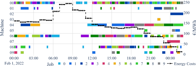

  

  Gantt diagram for mk06 with a makespan of 104 and €5053.61 energy costs

• (2) If decision makers are willing to accept a longer makespan in favor of lower energy costs, the potential of the memetic NSGA-II for reducing energy costs becomes more apparent. Figure 12 shows a solution for the instance mk06 with a makespan of 104 time steps (26 h), which is about 50% more time than in the schedule of Fig. 11. While the latter allows only small shifts of operations to favorable time periods, the solution with 104 time steps has a larger action space for shifting operations to times of favorable energy prices. Machines 01, 04, and 06 are still highly utilized, except that during the most expensive period between 6 and 11 a.m., only a few operations are processed. During the most expensive period between 7 and 9 a.m., there is no production on any machine. The schedule reduces the total energy costs to €5053.61, which is a saving of almost 40% compared to the schedule shown in Fig. 11.

  Fig. 13

  

  Gantt diagram for mk06 with a makespan of 512 and €745.70 energy costs

• (3) If decision makers place little emphasis on makespan and more on low energy costs, Fig. 13 shows a schedule with a makespan of 512 (5 days and 4 h), i.e. almost a whole week is available for production planning. In February, days 2nd, 5th and 6th have the most favorable energy prices for production in the period under consideration. All production is assigned to these days, while there is no production on other days. While the processing time increases by 642% compared to the schedule in Fig. 11, the total energy cost decreases by 91.1% to €745.70.

Overall, the results show how decision makers can use the different schedules to shape their production according to their interests. The Pareto front for the instance mk06 generated by the NSGA-II includes schedules for both time and energy cost-oriented objectives, allowing individual emphasis to be taken into account. If decision makers prefer to complete jobs quickly, they can select an appropriate production schedule from the Pareto front in the minimum makespan region and benefit from early completion. If decision makers prefer low energy cost production and can compensate for lower utilization, they can choose from schedules with longer makespan and higher energy cost savings. In both cases, decision makers can use the Pareto front to choose the schedule that meets their preferences.

6 Conclusion

In this section, we summarize our contribution and its limitation and provide an outlook on future research avenues.

6.1 Summary

Our study addresses the challenge of manufacturers to schedule their production according to both, minimum makespan and minimum energy costs assuming RTP tariffs. Based on requirements from literature and data from the German wholesale energy market, we formulate a linear optimization model that considers an FJSP with dynamic energy cost. To guide decision makers, we design a novel memetic NSGA-II that provides Pareto fronts for given orders and energy prices. In computational experiments, we analyze the effect of the memetic extension of the NSGA-II and compare the solution quality of the memetic NSGA-II with an exact state-of-the-art solver. We found the proposed greedy heuristic as a local refinement strategy helps to improve the calculated Pareto fronts of the memetic NSGA-II. Thereby, its Pareto fronts estimated in 45 min contain solutions that Gurobi does not find even after 12 h of runtime. Finally, we also show how manufacturers can set different emphases in terms of makespan and energy costs for their schedules by weighing the trade-off. This enables manufacturers to shape their production schedule according to individual demands and to process their jobs according within the preferred makespan and energy costs.

6.2 Limitations and future research

Based on the insights from this work, we have the following suggestions for future research. First, we recommend to identifying and integrating additional requirements from manufacturers and evaluating the memetic NSGA-II on real instances. In their review, Zhang et al. (2019) list studies in the field of job shop scheduling that consider requirements such as due dates, maximum delays, or material availability. Requirements can be extracted from interviews with manufacturers and added to the model as new constraints. While we evaluate the memetic NSGA-II using benchmark instances with real energy prices, further work can evaluate the NSGA-II using real-world instances. A case study could conclude potential savings and derive implications for practitioners on how they can benefit from an energy cost-aware scheduling.

A second avenue of research can explore alternative objectives for the FJSP. While we focus on energy costs from an economic point of view, we do not consider the sources of the energy consumed. Although a high level of energy production from sustainable sources could provide incentives for consumption through low costs, we see potential for a more precise consideration of the energy mix from an environmental point of view. In terms of green scheduling, Zheng and Wang (2016) and Xue et al. (2019) minimize makespan along with carbon emissions. Modifying our objective functions or expanding the problem to include a third objective could minimize the emissions caused by production, thus helping to find both economically and environmentally preferable solutions.

A third line of research may extend our approach to include a stochastic treatment of energy prices. Golari et al. (2017) addresses a scheduling problem for a production facility that minimizes the production costs. They formulate a stochastic model to account for uncertainties in renewable energy production. Bohlayer et al. (2018) consider large price fluctuations in energy markets and investigate how a stochastic MILP could be used to minimize the expected cost of purchasing energy. Similar to these approaches, our model could be extended to include energy price uncertainty. Further research could investigate how an improved energy price assumption affects the eventual cost of production. The results could guide manufacturers to design low energy cost schedules under consideration of uncertain fluctuating energy prices.

A fourth line of research can elaborate on the choice of algorithm. It can be investigated how further specializations of the memetic NSGA-II change the solution behaviour, such as a higher degree of customisation regarding the selection of individuals for crossover or the mutations. The algorithm can also be compared against with algorithms, such as SPEA2+ (Kim et al. 2004) or NTGA2 (Myszkowski and Laszczyk 2021). Further work could analyze which solution method is superior depending on the instance properties.

Appendices

Appendix 1 Energy cost calculation

In this section, we explain the design of the energy cost parameter $\eta _{ijkt}$, which specifies the individual energy costs for a given operation (i, j) on a machine k for a start time t. For the example calculation, we assume that one hour consists of four time steps. In Fig. 14, an example wholesale price for electricity $\kappa _t$ in Euros per MWh is plotted as a dashed line, with the price changing every four time steps (i.e., every hour). An operation (i, j) is assumed to be processed on a given machine k, which is associated with process time and energy consumption. The process time is given by the parameter $\tau _{ijk}$. For the example, the energy consumption of the machine k is assumed to be one megawatt for the operation (i, j).

Fig. 14

Example for calculating individual energy costs $\eta _{ijkt}$

To determine the individual price for the operation (i, j), the costs of each time step are added together and averaged, see Eq. (16). In addition, the resulting energy cost must be adjusted for the duration of the process, since the cost per megawatt-hour is given, but the process duration $\tau _{ijk}$ may be different. If the process duration $\tau _{ijk}$ exceeds the maximum time $t^{max}$ when started at t, $\eta _{ijkt}$ is infinite (or a very high value). So we allow infeasible solutions, but any other solution without exceeding the time limit is preferred.

$$\begin{aligned} \eta _{ijkt} = {\left\{ \begin{array}{ll} \frac{\sum _t^{\tau _{ijk}} \kappa _t}{\tau _{ijk}} \cdot \frac{\tau _{ijk}}{4} = \frac{\sum _t^{\tau _{ijk}} \kappa _t}{4}, &{} \text {if } t + \tau _{ijk} \ge t^{max} \\ \infty , &{} \text {otherwise} \end{array}\right. } \end{aligned}$$

(16)

In the example in Fig. 14, the operation (i, j) has a process time $\tau _{ijk}$ of 2, which is half an hour. Therefore, the price per megawatt-hour is halved. The solid line of Fig. 14 gives the resulting energy cost $\eta _{ijkt}$ for the operation (i, j) in machine k for each time step $t\in [0,20]$. As a parameter, $\eta _{ijkt}$ is customizable, so that individual machine costs, a base consumption, setup costs or other factors can be included as desired.

Appendix 2 Mutation operators

In this section, we explain the mutation operators used. In total, we use four different mutation operators: one each for the sequence and machine gene strings, and two for the energy cost gene string.

Fig. 15

Mutation of sequence and machine gene strings

Figure 15 shows the mutation operators for the sequence and machine gene strings. In the case of the sequence gene string, two genes with different values are randomly selected and swapped with each other. This affects the order in which the operations of the jobs are decoded into a schedule. For the machine gene string, one gene that specifies the machine assignment is randomly selected and replaced by another permissible machine. This can change the associated process time and the associated energy costs. Depending on the machine utilization, this can also lead to a changed makespan.

Fig. 16

Mutation of energy gene strings

For the energy cost string, replacing one gene of the energy cost gene string has little effect, so the entire energy cost string is replaced here. Figure 16 shows the two mutation operators. The energy cost gene mutation I has the goal of specifying the low cost values in order to generate low cost schedules. Conversely, the energy cost gene mutation II prefers high values to enable faster scheduling during decoding and to generate schedules with low makespan.

Fig. 17

Triangle distribution for mutating energy gene strings

When mutating the energy cost gene string, we use a triangular distribution to generate small and large values as shown in Fig. 17. The dashed line indicates the distribution for generating low energy costs, while the dotted line indicates that for generating high energy costs. The lower bound a is the minimum energy cost value $\eta _{ijkt}$ over all time steps t for a given operation (i, j) on a given machine k. The value b is the maximum energy cost value. The upper bound used for the triangular distribution is 0.75b and 1.5b for the energy cost gene string mutations I and II, respectively.

Appendix 3 Parameter configuration

The choice of parameters affects the solution quality of evolutionary algorithms. To prevent arbitrary parameter choices, tuning algorithms can be used to guide parameter choices and achieve better results. Tuning parameters is time- and resource-intensive and is especially suitable for repetitive problems, e.g. when decision makers have to solve almost the same problem instance every day (Eiben and Smit 2011).

Since we use different instances in our experiments and do not solve the same instance frequently, we do not perform parameter tuning. However, to avoid randomly choosing a bad parameterization, we test different parameter configurations beforehand using instance mk05. We choose instance mk05 because it is a medium-sized instance with 15 jobs and 5–10 operations per job. Table 8 shows the values used for the parameter configuration tests. We test all combinations of different specifications of population size n, tournament size ts, tournament winners tw, and mutation rates ms, mm, and me. In total, $3 \cdot 3 \cdot 2 \cdot 3 = 54$ different configurations were tested.

Table 8 Parameter configurations

To evaluate the quality of the parameter configuration, we consult the extrema of the generated best found Pareto fronts, i.e. the minimum makespan and energy cost per run. Both objective values are normalized to a scale of 0 to 1 and summed to give each solution a score ranging from 0 to 2.

For the 54 parameter configuration tests, solutions with population sizes n of 300, 700, and 1000 individuals have an average score of 1.01, 0.95, and 1.11, respectively. Solutions with a tournament size ts of 0.5, 0.6, and 0.7 have an average score of 1.12, 0.95, and 1.00, respectively. Solutions with a relative tournament size tw of 0.15 and 0.3 have an average score of 1.06 and 0.99. Solutions with a mutation rate ms, mm and me have an average score of 1.06, 0.97 and 1.04.

Overall, among all tested solutions, those with a parameter configuration of $n=700$, $ts=0.6$, $tw=0.3$, and $ms, mm, me=0.2$ score the lowest, so we adopted this parameter configuration for our experimental settings (cf. Sect. 5.1).

Appendix 4 Pareto fronts

In this section, we present the Pareto fronts of all instances as a complement to Sect. 5.4. The solutions on the Pareto front of the memetic NSGA-II are marked with $+$. Different color gradients distinguish the different runs. The x-axis shows the makespan in 15-minute increments, while the y-axis shows the energy cost of each solution. To determine the distance of a solution from the optimum, we estimate an optimal Pareto front using the epsilon-constraint method described in Sect. 3. We estimate the optimal Pareto front by setting the epsilon to the fastest makespan found by the memetic algorithm after 45 min and incrementing it to the slowest makespan found. The estimation of the optimal Pareto front consists of 15 x-axis sections. Orange downward triangles mark the best solution (incumbent) found by Gurobi, while red upward triangles mark the best bound found. A red mark on the x-axis means that no result could be computed with the epsilon-constraint method for this x-axis segment.

See Figs. 18, 19, 20, 21, 22, 23, 24, 25, 26, 27, 28, 29, 30, 31 and 32.

Fig. 18

Pareto front of mk01

Fig. 19

Pareto front of mk02

Fig. 20

Pareto front of mk03

Fig. 21

Pareto front of mk04

Fig. 22

Pareto front of mk05

Fig. 23

Pareto front of mk06

Fig. 24

Pareto front of mk07

Fig. 25

Pareto front of mk08

Fig. 26

Pareto front of mk09

Fig. 27

Pareto front of mk10

Fig. 28

Pareto front of mk11. The computations of the instance mk11 with the epsilons of 693 and 769 time steps were aborted early due to insufficient memory

Fig. 29

Pareto front of mk12

Fig. 30

Pareto front of mk13. The computations of the instance mk13 with the epsilons of 438 and 608 time steps were aborted early due to insufficient memory

Fig. 31

Pareto front of mk14. The computations of the instance mk14 with the epsilon of 2128 time steps was aborted early due to insufficient memory

Fig. 32

Pareto front of mk15. The computations of the instance mk15 with the epsilons of 389, 471, and 2036 time steps were aborted early due to insufficient memory

References

Abikarram JB, McConky K, Proano R (2019) Energy cost minimization for unrelated parallel machine scheduling under real time and demand charge pricing. J Clean Prod 208:232–242. https://doi.org/10.1016/j.jclepro.2018.10.048
Abujarad SY, Mustafa M, Jamian J (2017) Recent approaches of unit commitment in the presence of intermittent renewable energy resources: a review. Renew Sustain Energy Rev 70:215–223. https://doi.org/10.1016/j.rser.2016.11.246
Biel K, Zhao F, Sutherland JW et al (2018) Flow shop scheduling with grid-integrated onsite wind power using stochastic MILP. Int J Prod Res 56(5):2076–2098. https://doi.org/10.1080/00207543.2017.1351638
Bohlayer M, Fleschutz M, Braun M et al (2018) Demand side management and the participation in consecutive energy markets-a multistage stochastic optimization approach. In: 2018 15th international conference on the european energy market (EEM). IEEE, pp 1–5. https://doi.org/10.1109/EEM.2018.8469912
Brandimarte P (1993) Routing and scheduling in a flexible job shop by tabu search. Ann Oper Res 41(3):157–183. https://doi.org/10.1007/BF02023073
Carlucci D, Renna P, Materi S (2021) A job-shop scheduling decision-making model for sustainable production planning with power constraint. IEEE Trans Eng Manag. https://doi.org/10.1109/TEM.2021.3103108
Che A, Zhang S, Wu X (2017) Energy-conscious unrelated parallel machine scheduling under time-of-use electricity tariffs. J Clean Prod 156:688–697. https://doi.org/10.1016/j.jclepro.2017.04.018
Dai M, Tang D, Giret A et al (2019) Multi-objective optimization for energy-efficient flexible job shop scheduling problem with transportation constraints. Robot Comput Integr Manuf 59:143–157. https://doi.org/10.1016/j.rcim.2019.04.006
Das I (1999) On characterizing the "knee’’ of the pareto curve based on normal-boundary intersection. Struct Optim. 18:107–115. https://doi.org/10.1007/BF01195985
Deb K, Jain H (2013) An evolutionary many-objective optimization algorithm using reference-point-based nondominated sorting approach, part I: solving problems with box constraints. IEEE Trans Evol Comput 18(4):577–601. https://doi.org/10.1109/TEVC.2013.2281535
Deb K, Pratap A, Agarwal S et al (2002) A fast and elitist multiobjective genetic algorithm: NSGA-II. IEEE Trans Evol Comput 6(2):182–197. https://doi.org/10.1109/4235.996017
D’Ettorre F, Banaei M, Ebrahimy R et al (2022) Exploiting demand-side flexibility: state-of-the-art, open issues and social perspective. Renew Sustain Energy Rev 165(112):605. https://doi.org/10.1016/j.rser.2022.112605
Dhakal S, Minx J, Toth F et al (2022) IPCC, 2022: Climate Change 2022: Mitigation of Climate Change. Contribution of Working Group III to the Sixth Assessment Report of the Intergovernmental Panel on Climate Change. Cambridge University Press, chap Emissions Trends and Drivers. https://doi.org/10.1017/9781009157926.004
Eiben AE, Smit SK (2011) Parameter tuning for configuring and analyzing evolutionary algorithms. Swarm Evol Comput 1(1):19–31. https://doi.org/10.1016/j.swevo.2011.02.001
Eid C, Koliou E, Valles M et al (2016) Time-based pricing and electricity demand response: existing barriers and next steps. Util Policy 40:15–25. https://doi.org/10.1016/j.jup.2016.04.001
European Commission (2019) The European Green Deal. Communication from the Commission to the European Parliament, the European Council, the Council, the European Economic and Social Committee and the Committee of the Regions COM (2019) 640 final
Fang K, Uhan N, Zhao F et al (2011) A new approach to scheduling in manufacturing for power consumption and carbon footprint reduction. J Manuf Syst 30(4):234–240. https://doi.org/10.1016/j.jmsy.2011.08.004
Fazli Khalaf A, Wang Y (2018) Energy-cost-aware flow shop scheduling considering intermittent renewables, energy storage, and real-time electricity pricing. Int J Energy Res 42(12):3928–3942. https://doi.org/10.1002/er.4130
Federal Network Agency Germany (2022) SMARD market data. https://www.smard.de/en/downloadcenter/download-market-data
Gandhi O, Rodríguez-Gallegos CD, Srinivasan D (2016) Review of optimization of power dispatch in renewable energy system. In: 2016 IEEE innovative smart grid technologies—Asia (ISGT-Asia), pp 250–257. https://doi.org/10.1109/ISGT-Asia.2016.7796394
Gendreau M, Potvin JY et al (2010) Handbook of metaheuristics, vol 2. Springer, Berlin. https://doi.org/10.1007/978-1-4419-1665-5
Golari M, Fan N, Jin T (2017) Multistage stochastic optimization for production-inventory planning with intermittent renewable energy. Prod Oper Manag 26(3):409–425. https://doi.org/10.1111/poms.12657
Gong G, Deng Q, Gong X et al (2018) A new double flexible job-shop scheduling problem integrating processing time, green production, and human factor indicators. J Clean Prod 174:560–576. https://doi.org/10.1016/j.jclepro.2017.10.188
Gong G, Deng Q, Gong X et al (2021) A non-dominated ensemble fitness ranking algorithm for multi-objective flexible job-shop scheduling problem considering worker flexibility and green factors. Knowl Based Syst 231(107):430. https://doi.org/10.1016/j.knosys.2021.107430
Gong X, De Pessemier T, Joseph W et al (2015) An energy-cost-aware scheduling methodology for sustainable manufacturing. Procedia CIRP 29:185–190. https://doi.org/10.1016/j.procir.2015.01.041
Gong X, De Pessemier T, Joseph W et al (2016) A generic method for energy-efficient and energy-cost-effective production at the unit process level. J Clean Prod 113:508–522. https://doi.org/10.1016/j.jclepro.2015.09.020
Gong X, Deng Q, Gong G et al (2018) A memetic algorithm for multi-objective flexible job-shop problem with worker flexibility. Int J Prod Res 56(7):2506–2522. https://doi.org/10.1080/00207543.2017.1388933
Haimes Y (1971) On a bicriterion formulation of the problems of integrated system identification and system optimization. IEEE Trans Syst Man Cybern SMC 1(3):296–297. https://doi.org/10.1109/TSMC.1971.4308298
International Energy Agency (2022) Renewables 2022. https://www.iea.org/reports/renewables-2022. Accessed 13 Mar 2023
Jiang T, Zhang C, Sun QM (2019) Green job shop scheduling problem with discrete whale optimization algorithm. IEEE Access 7:43153–43166. https://doi.org/10.1109/ACCESS.2019.2908200
Kemmoé S, Lamy D, Tchernev N (2015) A job-shop with an energy threshold issue considering operations with consumption peaks. IFAC PapersOnLine 48(3):788–793. https://doi.org/10.1016/j.ifacol.2015.06.179
Kim M, Hiroyasu T, Miki M, et al (2004) Spea2+: improving the performance of the strength pareto evolutionary algorithm 2. In: Parallel problem solving from nature-PPSN VIII: 8th international conference, Birmingham, UK, 18–22 Sept, 2004. Proceedings 8. Springer, pp 742–751. https://doi.org/10.1007/978-3-540-30217-9_75
Lu C, Zhang B, Gao L et al (2021) A knowledge-based multiobjective memetic algorithm for green job shop scheduling with variable machining speeds. IEEE Syst J 16(1):844–855. https://doi.org/10.1109/JSYST.2021.3076481
Masmoudi O, Delorme X, Gianessi P (2019) Job-shop scheduling problem with energy consideration. Int J Prod Econ 216:12–22. https://doi.org/10.1016/j.ijpe.2019.03.021
Moon JY, Park J (2014) Smart production scheduling with time-dependent and machine-dependent electricity cost by considering distributed energy resources and energy storage. Int J Prod Res 52(13):3922–3939. https://doi.org/10.1080/00207543.2013.860251
Moscato P, Cotta C (2003) A gentle introduction to memetic algorithms. Handbook of metaheuristics. Springer, Berlin, pp 105–144. https://doi.org/10.1007/0-306-48056-5_5
Myszkowski PB, Laszczyk M (2021) Diversity based selection for many-objective evolutionary optimisation problems with constraints. Inf Sci 546:665–700. https://doi.org/10.1016/j.ins.2020.08.118
Özgüven C, Özbakır L, Yavuz Y (2010) Mathematical models for job-shop scheduling problems with routing and process plan flexibility. Appl Math Model 34(6):1539–1548. https://doi.org/10.1016/j.apm.2009.09.002
Piroozfard H, Wong KY, Wong WP (2018) Minimizing total carbon footprint and total late work criterion in flexible job shop scheduling by using an improved multi-objective genetic algorithm. Resour Conserv Recycl 128:267–283. https://doi.org/10.1016/j.resconrec.2016.12.001
Rahimi I, Gandomi AH, Deb K et al (2022) Scheduling by NSGA-II: review and bibliometric analysis. Processes. https://doi.org/10.3390/pr10010098
Shrouf F, Ordieres-Meré J, García-Sánchez A et al (2014) Optimizing the production scheduling of a single machine to minimize total energy consumption costs. J Clean Prod 67:197–207. https://doi.org/10.1016/j.jclepro.2013.12.024
Tang D, Dai M (2015) Energy-efficient approach to minimizing the energy consumption in an extended job-shop scheduling problem. Chin J Mech Eng 28(5):1048–1055. https://doi.org/10.3901/CJME.2015.0617.082
Urselmann M, Barkmann S, Sand G et al (2011) Optimization-based design of reactive distillation columns using a memetic algorithm. Comput Chem Eng 35(5):787–805. https://doi.org/10.1016/j.compchemeng.2011.01.038
Vallejos-Cifuentes P, Ramirez-Gomez C, Escudero-Atehortua A et al (2019) Energy-aware production scheduling in flow shop and job shop environments using a multi-objective genetic algorithm. Eng Manag J 31(2):82–97. https://doi.org/10.1080/10429247.2018.1544798
Vamplew P, Yearwood J, Dazeley R et al (2008) On the limitations of scalarisation for multi-objective reinforcement learning of pareto fronts. In: AI 2008: advances in artificial intelligence: 21st Australasian joint conference on artificial intelligence, Auckland, New Zealand, 1–5 Dec, 2008. Proceedings 21. Springer, pp 372–378. https://doi.org/10.1007/978-3-540-89378-3_37
Verma S, Pant M, Snasel V (2021) A comprehensive review on NSGA-II for multi-objective combinatorial optimization problems. IEEE Access 9:57757–57791. https://doi.org/10.1109/ACCESS.2021.3070634
Wang B, Xie H, Xia X et al (2018) A NSGA-II algorithm hybridizing local simulated-annealing operators for a bi-criteria robust job-shop scheduling problem under scenarios. IEEE Trans Fuzzy Syst 27(5):1075–1084. https://doi.org/10.1109/TFUZZ.2018.2879789
Wang L et al (2020) Multi-objective optimization based on decomposition for flexible job shop scheduling under time-of-use electricity prices. Knowl Based Syst 204(106):177. https://doi.org/10.1016/j.knosys.2020.106177
Wang S, Mason SJ, Gangammanavar H (2020) Stochastic optimization for flow-shop scheduling with on-site renewable energy generation using a case in the united states. Comput Ind Eng 149(106):812. https://doi.org/10.1016/j.cie.2020.106812
Wu X, Sun Y (2018) A green scheduling algorithm for flexible job shop with energy-saving measures. J Clean Prod 172:3249–3264. https://doi.org/10.1016/j.jclepro.2017.10.342
Xue Y, Rui Z, Yu X et al (2019) Estimation of distribution evolution memetic algorithm for the unrelated parallel-machine green scheduling problem. Memet Comput 11:423–437. https://doi.org/10.1007/s12293-019-00295-0
Yin L, Li X, Gao L et al (2017) A novel mathematical model and multi-objective method for the low-carbon flexible job shop scheduling problem. Sustain Comput Inf Syst 13:15–30. https://doi.org/10.1016/j.suscom.2016.11.002
Yuan Y, Xu H, Wang B et al (2015) A new dominance relation-based evolutionary algorithm for many-objective optimization. IEEE Trans Evol Comput 20(1):16–37. https://doi.org/10.1109/TEVC.2015.2420112
Zhang H, Zhao F, Fang K et al (2014) Energy-conscious flow shop scheduling under time-of-use electricity tariffs. CIRP Ann 63(1):37–40. https://doi.org/10.1016/j.cirp.2014.03.011
Zhang H, Zhao F, Sutherland JW (2015) Energy-efficient scheduling of multiple manufacturing factories under real-time electricity pricing. CIRP Ann 64(1):41–44. https://doi.org/10.1016/j.cirp.2015.04.049
Zhang J, Ding G, Zou Y et al (2019) Review of job shop scheduling research and its new perspectives under industry 4.0. J Intell Manuf 30:1809–1830. https://doi.org/10.1007/s10845-017-1350-2
Zheng XL, Wang L (2016) A collaborative multiobjective fruit fly optimization algorithm for the resource constrained unrelated parallel machine green scheduling problem. IEEE Trans Syst Man Cybern Syst 48(5):790–800. https://doi.org/10.1109/TSMC.2016.2616347
Funding
Open Access funding enabled and organized by Projekt DEAL. The authors gratefully acknowledge the financial support provided by the state of North Rhine-Westphalia, Germany, as part of the progres.nrw program area, in the framework of Re²Pli (project number EFO 0127A) and the funding of this project by computing time provided by the Paderborn Center for Parallel Computing (PC²).
Author information
Authors and Affiliations
Corresponding author
Ethics declarations
Conflict of interest
The authors have no relevant financial or non-financial interests to disclose.
Additional information
Publisher's Note
Springer Nature remains neutral with regard to jurisdictional claims in published maps and institutional affiliations.
The article has been corrected to update fig 18 and some information for specific instances (mk11, mk13, mk14, mk15).