
Abstract
Current interest into past climate change and its potential role for changes in the environment call for spatially distributed climate datasets of high temporal resolution and extending over several decades. To foster such research, we present a new gridded dataset of daily minimum and maximum temperature covering Austria at 1-km resolution and extending back till 1961 at daily time resolution. To account for the complex and highly variable thermal distributions in this high-mountain region, we adapt and employ a recently published interpolation method that estimates nonlinear temperature profiles with altitude and accounts for the non-Euclidean spatial representativity of station measurements. The spatial analysis builds upon 150 station series in and around Austria (homogenised where available), all of which extend over or were gap-filled to cover the entire study period. The restriction to (almost) complete records shall avoid long-term inconsistencies from changes in the station network. Systematic leave-one-out cross-validation reveals interpolation errors (mean absolute error) of about 1 °C. Errors are relatively larger for minimum compared to maximum temperatures, for the interior of the Alps compared to the flatland and for winter compared to summer. Visual comparisons suggest that valley-scale inversions and föhn are more realistically captured in the new compared to existing datasets. The usefulness of the presented dataset (SPARTACUS) is illustrated in preliminary analyses of long-term trends in climate impact indices. These reveal spatially variable and eventually considerable changes in the thermal climate in Austria.
1 Introduction
1.1 Context
There is a brisk demand on national meteorological services and other data providers to offer spatially comprehensive datasets of the observed climate in daily time resolution and extending over several decades. Applications in environmental planning and climate impact research require knowledge of the temporal course of a climate variable either at specific locations remote from observation stations or averaged over defined geographic entities. This type of climate information is required as input for quantitative models of environmental or societal systems. Common applications in climate impact research, official planning and hazard management include modelling, reanalysis, monitoring or forecasting of drought and fire danger (e.g. Haslinger et al. 2014; Petritsch and Hasenauer 2014), of snow cover, glacier mass balance and runoff (e.g. Olefs et al. 2013; Huss et al. 2008; Massmann and Holzmann 2012) and of vegetation growth, crop growth and pest spread (e.g. Kapeller et al. 2012; Seidl et al. 2009). In climate research itself, gridded datasets provide a basis to monitor and analyse trends and variations of basic climate variables including impact-related climate indices (e.g. Chimani et al. 2013; Donat et al. 2013), they serve as reference for evaluating regional climate models (e.g. Haslinger et al. 2013) and they are an important ingredient in the development of high-resolution regional climate change scenarios (e.g. Themeßl et al. 2011). In all the mentioned applications, near-surface air temperature is an indispensable quantity.
Meteorological services of many European countries now offer area-covering data products in the form of a chronology of regular grids. These supplement the traditional in situ data products consisting of observational time series at climate stations. To interpolate climate variables from in situ temperature measurements onto a continuous grid, spatialisation methods have been designed over the last decades, which take account of the peculiarities of climate variables. Frequently used methods for (temperature) interpolation on a regional and daily basis are the following: (1) The method PRISM (parameter-elevation relationships on independent slopes model) has been developed by Daly et al. (1994; 2008). It relies on localised, geographically weighted regressions, with piecewise linear parameter-altitude relationships estimated at each grid point of a digital elevation model (DEM). The regression involves the most representative observation stations for the target grid point, via a weighting scheme taking into account several physiographic conditions. (2) Bénichou and Le Breton (1987) presented the AUREHLY (analyse utilisant le relief pour l’hydrométéorologie) method, which, apart from elevation, also uses patterns of the neighbourhood topography in the form of principal components as predictors in a multiple linear regression. The remaining station residuals are interpolated by kriging. The method has been applied in numerous applications at monthly, yearly and climatological time resolutions. (3) MISH (meteorological interpolation based on surface homogenised data basis) by Szentimrey et al. (2011) is a regression- and kriging-based method. The climate statistical parameters that determine the favourable interpolation parameters by error reduction are modelled with the help of auxiliary variables like horizontal distance, topography and principal component fields of topography. Its characteristic feature lies in the application of the whole climate series for modelling, i.e. considering a sample in time and space. (4) The interpolation tool Daymet was introduced by Thornton et al. (1997). It combines local multilinear regression with a Gaussian distance weighting, somewhat similar to PRISM, but with less sophistication in physiographic predictors. Daymet is targeted for daily time resolution and is used a lot in agricultural and ecosystem applications (e.g. Hasenauer et al. 2003; Ruefenacht et al. 2008). (5) VERA (Vienna enhanced resolution analysis) is a multiparameter mesoscale analysis tool developed with a focus on data quality control and model evaluation in mountain regions (Steinacker et al. 2011; Bica et al. 2007). It is based on a variational approach using thin-plate splines and fingerprint patterns that represent small-scale thermal effects from typical mountain weather phenomena (Steinacker et al. 2006). (6) Recently, Frei (2014) presented a method, specifically developed for the interpolation of temperature in mountainous study regions. It superimposes macroclimatic background fields based on nonlinear vertical profiles with mesoclimatic residual fields based on non-Euclidean distance weighting. This method is described in more detail in Section 3.1. (7) Analyses (or reanalyses) based on dynamic meteorological models are an alternative data source on spatially complete climate information (e.g. Haiden et al. 2011; Luhamaa et al. 2011; Rienecker et al. 2011). Physical and dynamical equations as well as the volume of observational input provide additional constraints that are not exploited in a purely statistical interpolation. The resolution of currently available regional reanalyses is still coarse and their consistency regarding long-term climatic variations has yet to be verified (e.g. Bukovsky and Karoly 2007; Isotta et al. 2014).
During the last years, several gridded temperature datasets have been created for the territory of Austria by adaption of the above methods: (1) Schöner and Dos Santos Cardoso (2004) applied the AUREHLY procedure upon about 70 quality-controlled, continuous station series. The resulting StartClim dataset has daily resolution and extends over the period 1948–2007. (2) Hasenauer et al. (2003) adapted the Daymet method in Austria, mainly for purposes of local forest ecosystem modelling and fire danger assessment. The dataset starts in 1960 and has been updated until 2012, relying on a temporarily variable network of between 192 and 285 stations. (3) INCA (Integrated nowcasting through comprehensive analysis) is the numerical weather analysis and nowcasting model of the Austrian meteorological service ZAMG (Haiden et al. 2011). Output is available for the period since 2006, yet it is subject to frequent variations in data input (including up to 550 temperature observations) and changes in algorithm. It has served as a valuable reference for cross-checking grid datasets based purely on statistical interpolation.
All existing datasets provide valuable data sources for numerous applications. However, for the analysis of weather-scale temperature variations over climatological time scales, they are either too short in extent (e.g. INCA), lack daily resolution (e.g. monthly in HISTALP; Chimani et al. 2013), are not continuously updated (e.g. StartClim) or they are subject to large variations in input data and/or methods that compromise their long-term consistency (e.g. Daymet, INCA).
1.2 Concept
In a situation with temporally highly variable station networks, there arise difficulties in meeting the two primary requirements of best possible spatial resolution and long-term consistency with one single grid dataset. High spatial resolution calls for integrating all available observational information at any particular point in time. But the associated variations in network density are likely to lead to temporal variations in the error structure of the interpolation, which can result in artificial trends or step inhomogeneities. Examples of such artefacts are illustrated, for example, in Frei (2014) and Masson and Frei (2014). Alternatively, interpolation methods that ought to be resistant against large variations in station density (e.g. Masson and Frei 2014) are unlikely to exploit the full spatial information available during periods with dense observation.
These circumstances led to the development of the new temperature dataset for Austria, presented in this article. The primary ambition is to achieve best possible consistency over climatological time scales while making compromises to effective spatial resolution. This is attempted by restricting to observational series that are almost complete over the targeted period (1961 to present), by adopting a procedure to fill remaining data gaps and, finally, by interpolating from the resulting stationary station network. The parameters of interest are daily minimum (Tn) and maximum temperature (Tx) and the grid spacing is 1 km. The daily temperature extremes are important inputs for the study of climate sensitivities in environmental systems (e.g. vegetation, glaciers), they are the basis for many derived climate change indices (cf. Klein Tank et al. 2009) and they permit for an approximate estimate of daily mean temperature (cf. section 2.2 in Hiebl et al. 2009). The dataset will be updated continuously and, hence, provides an ideal element of a national climate service to monitor the evolution in surface temperature, including the occurrence of extreme conditions, and to relate this to the past.
As method of spatial interpolation, we have chosen the methodology of Frei (2014). This is motivated by the fact that the complex topography of Austria spawns similar mountain-related weather phenomena like in Switzerland, the area this method has been originally developed for. Its construction principles are made to account for sharp across-ridge contrasts, nonlinear vertical profiles, valley-scale cold-pools and föhn, challenges similarly met in Austria. However, the method required considerable configuration work and adaptations to the geographic conditions and network density in Austria.
In the reminder of the paper, we describe the dataset and the gap-filling procedure adopted (Section 2). Section 3 explains the principles of the interpolation method and details the configuration and adaptations made for the territory of Austria. In Section 4, we present the example of a challenging thermal distribution to illustrate the working of the interpolation, discuss results from a systematic cross-validation and compare results from the newly developed dataset to existing datasets. As an illustration of its potential applications, we discuss trends in selected climate impact indicators derived from the new dataset. The paper concludes with Section 5.
2 Data
2.1 Station selection
Like in many other countries, the climatological measurement network in Austria exhibits substantial variations in station density over time. This is illustrated in Fig. 1, showing the evolution of available daily Tn observations (a similar situation is found for daily Tx), During the period 1961–2012, between 180 and 275 stations were in operation at any particular day (black line). But the total station number is only partly indicative of the numerous closings and new installations. The number of stations with a continuous series over the 52 years is only 98 (full green line). And the total count of stations operated at any instant in the period is as large as 428 (dashed red line). The rate of station closings (slope of dashed red line) and the rate of station openings (slope of dashed green line) are approximately constant over time. There are many practical reasons for changes in a station network but over time this imposes a significant limitation for the quality of climatological analyses. For our application, a compromise had to be found between affordable gaps in time (to be filled later) and desired resolution in space. Our conservative choice (small rate of gaps) was to incorporate all series with less than 5 % missing values during the 52 years 1961–2012 considered. This resulted in a total of 112 stations from which both Tn and Tx were used in the construction of the daily grids. At ZAMG, daily Tn and Tx are defined to be the extremes over the 24-h-span between 19:00 of the previous day and 19:00 of the current day.

Number of daily minimum temperature (Tn) observations available from the Austrian meteorological station network between 1961 and 2012. The total number of Tn stations in operation each year is depicted as black line. Solid coloured lines indicate the number of stations with continuous measurements (less than 15 days missing per year) since the beginning (1961, green) and until the end (2012, red). Dashed lines indicate the number of stations with at least some measurements since the beginning (1961, green) and until the end (2012, red). Decreases in the red lines exhibit discontinuations of stations, increases in the green lines exhibit new installations
All the data from the selected stations have been tested by the operational data quality control procedures at ZAMG. Moreover, 52 out of the 112 station series were subject to detailed tests and adjustments for climatological inhomogeneities. These station series were taken from Nemec et al. (2013), who compiled a dataset of homogenised daily Tn and Tx (and precipitation sum) observations by applying the homogenisation procedures by Caussinus and Mestre 2004 (PRODIGE) and Mestre et al. 2011 (SPLIDHOM) to Austrian station series. The remaining data series remain unhomogenised.
To avoid degradation in mapping quality in border-near regions of Austria, it was necessary to include daily observations from the eight neighbouring countries. For the period 1961–2012, another 38 daily station series obtained from foreign institutions could be integrated in our processing. From 2013 onwards, these series are updated by taking advantage of the regular international data exchange between meteorological services (SYNOP).
Altogether, the final input station dataset consists of 150 Tn and Tx (112 domestic and 38 foreign) series (Fig. 2). Metadata reviewing revealed that almost all series are subject to relocations. For those 25 Austrian series, which underwent an altitude shift by 30 m or more, the altitudinal shifts cannot be neglected. A correction of these shifts was made by estimating the mean annual course of the attendant inhomogeneity by comparison to a reference time series from high-correlated non-shifted stations in the neighbourhood. The data segment of the candidate station before the elevation shift was then adjusted by this mean signal to become more consistent with the more recent segment. Further potentially disturbing effects of station relocations have not been considered separately. Moreover, the daily data series have been adjusted such that their linear temporal trends for the period 1961–2010 are consistent to trends of the corresponding monthly series of the homogenised HISTALP dataset (Auer et al. 2007). If the linear trend estimated from the daily series deviates by more than 0.3 °C (over the 50-year period 1961–2010) from that of the corresponding monthly HISTALP series, an adjustment was made to the daily series, linear across the period and on the basis of yearly adjustment values, so that their linear trend is consistent with the HISTALP trend.

Network of daily Tn and Tx series used in and near Austria. Downward triangles mark stations at locations prone to cold-pool formation, upward triangles stations at summit locations, diamonds stations at inner-city locations and circles stations at all other locations. The subregions used for the vertical temperature profiles are mapped in colour (northwest green, northeast orange, south red). Colour intensity represents region weight (see Section 3.2)
2.2 Gap-filling
The consideration of almost complete time series in our application implies that there is considerable overlap of the fragmented time series with observations at neighbouring stations. As a result, there is scope to fill in these gaps more accurately by exploiting the joint observations compared to spatial interpolation alone. In order to keep the filling procedure flexible and repeatable, its design is simple and uses the complete temperature stations only. Gap-filling is operationally repeated after data enquiry every day over the entire study period, by removing previously gap-filled values and refilling all gaps considering the newly added observations.
Gap-filling is accomplished separately for Tn and Tx. The series are distinguished into reference series (almost) without any missing data and candidate series. For each candidate series, the three best correlated reference series are selected, whose (correlation-weighted) mean series serves as the actual reference series. Correlation on basis of the entire daily series proves to be an effective measure for the selection of close-by stations in a similar mesoclimatic setting (prone to cold-pools, on mountain summits, etc.). Next, the daily differences between the candidate and the actual reference series are averaged over the individual years to obtain a mean annual course of differences. The mean annual course of differences it smoothed using the mean over a 21-day running window. In case of a daily missing value in the candidate series, the value of the respective calendar day out of the smoothed mean annual course of differences is added on the daily value from the actual reference series, in order to fill the gap.
The gap-filling procedure was tested and evaluated by experiments where observed but retained observations were reconstructed. For both Tn and Tx, evaluation revealed no systematic bias with both the mean and the standard deviation of station-wise mean errors (ME) being smaller than 0.01 °C. The mean absolute error (MAE) is 1.0 °C and the mean root-mean-square error (RMSE) is 1.3 °C. The mentioned figures apply to the 112 Austrian stations. Errors tend to be slightly larger especially at relatively remote stations in the southern neighbouring countries. Gap-filling possibly leads to a smoothing of gap-filled in comparison to original data with possible implications for threshold-based climate indices. Over the entire length of the series, this effect is, however, small as the mean temperature standard deviation is reduced by only 0.05 %. Comparing gap-filled data sequences of sufficient length (>500 values) to original data sequences, the change in standard deviation comes to −2.1 %.
3 Interpolation
3.1 Method principles
The spatial analysis of daily Tn and Tx station observations onto the regular 1-km grid over Austria was accomplished by the interpolation method of Frei (2014), reconfigured for the territory of Austria. The method combines a macroclimatic background field, representing large-scale horizontal and basin-scale vertical temperature variations, with a mesoclimatic residual field, representing more local phenomena such as valley-scale cold-pools and warm föhn air layers in Alpine valleys.
The background field is constructed from a large-scale vertical temperature profile, varying smoothly in the horizontal and allowing for nonlinear vertical dependence, characteristic of basin-scale inversion layers and boundary-layer signatures (see Eq. (1) and Fig. 4 in Frei (2014)). The vertical profiles are determined for predefined but gradually overlapping subregions of the study domain. There is considerable flexibility in the parametric profile function that allows to model multilinear stratifications and inversions of different strength, height, and thickness. Valley stations, known to be frequently affected by smaller-scale cold-pools, are deliberately ignored in the estimation of the background profiles. Similar to Frei (2014), these cold-pool stations were identified by inspecting the mean diurnal temperature range (Tx minus Tn; cf. Fig. 2).
The residual field is constructed by weighting the station residuals from the background field. The weighting scheme is not strictly distance-related (Euclidean), but uses a predefined set of generalised distance fields determined from a non-Euclidean distance metric that takes account of the topographic obstruction of air-flows (see Eq. (4) and Fig. 5 in Frei (2014)). The metric has a free parameter, the layering coefficient λ. It describes the additional penalty in distance, incurred from changes in elevation and is expressed in meters per meter (i.e. dimensionless). The parameter varies from day to day and is determined in an error reduction procedure. The larger λ is, the stronger are topographic imprints in the residual interpolation. The case λ = 0 marks the Euclidean limit and is included in the set. Background and residual fields are finally superimposed to obtain the final temperature field.
Figure 3 depicts maps of the generalised distance valid for four example stations in Austria and for a layering coefficient of λ = 100 (i.e. a horizontal penalty of +100 m per 1 m elevation change). The corresponding Euclidean distance (λ = 0) is depicted for comparison. As for a valley floor station, locations along valley axis receive much smaller generalised distances than locations at the valley slopes and adjacent ridges (Fig. 3a). As a result, measurements from this station have a stronger influence in the interpolation at grid points along the valley than at grid points on slopes and ridges, even if the latter are much closer to the station in terms of Euclidean distance. For a summit station, the generalised distance field shows an interrupted pattern, with areas at comparable elevations being closer (Fig. 3b). Information from this station will be weighted more favourably at adjacent mountains massifs but strongly downweighted for locations in nearby valleys. In the case of a lowland station outside the Alps, the generalised distance field roughly keeps the concentric (Euclidean) structure in the open foreland, but distances are rapidly increased at the edge of the mountain ridge (Fig. 3c).

Generalised distance fields for layering coefficient λ = 100 for a valley station (a), a summit station (b), a foreland station (c) and an inner-city station (d). In the latter case, urban representativity has been integrated. Intense colouring means smaller generalised distance from the station. For comparison, Euclidean distance (λ = 0, in steps of 20 km) is drawn as grey circles. The map sections encompass areas of 200 × 200 km
This is just a brief outline of the interpolation method that should help to understand its configuration and procedural adaptations. A detailed description of the method with example applications is given in Frei (2014, see especially Sections 3 and 4.1).
3.2 Configuration and adaptations
The application of the interpolation method in this study could build on the original implementation of the software for Switzerland. The implementation is written in programming language R (R Core Team 2011). The transfer of the interpolation method to the situation in Austria, however, called for a careful configuration and several procedural adaptations that were found essential for the quality of temperature interpolations in Austria. In the following, we describe the configuration and method adaptations point by point:
-
Subregions of the background field: The background field of the method is based on vertical profiles estimated for subjectively predefined subregions and subsequently merged via gradual blending. The configuration in Austria therefore called for a suitable regional subdivision. It turned out that the simple north–south separation across the main Alpine crest, chosen in the application for Switzerland, was not satisfactory. Austria’s larger west-to-east extension called for a more refined regionalisation of the vertical temperature dependence in the background field. This was essential to avoid that horizontal temperature gradients spoil the vertical dependence. Therefore, the domain was zoned into three subregions, by dividing the area north of the main crest in the west–east direction. This was done by implementing a linear transition of subregion weights between the western and eastern edges of the domain. The resulting subregions are called northwest, northeast and south, respectively, and are depicted in Fig. 2. The three-part division clearly improves the result when there are larger-scale temperature patterns with marked longitudinal contrasts, such as those occurring with the passage of fronts.
-
Vertical profile fitting: The original scheme for estimating the parameters of the nonlinear vertical temperature profile proceeds in several steps towards minimising squared differences (nonlinear least squares). A critical point in the process is the estimation of a lapse rate for the top-most layer (i.e. above inversions). In the implementation for Switzerland, this was achieved in an iterative procedure from dedicated high-level stations, but with the possibility that some of them could be discarded when there were nonlinearities high up. This procedure turned out to be unfavourable for the application in Austria due to station distribution in combination with the country’s geography. The common problem that low-level stations are overrepresented is augmented by the instance, that Austria’s mean altitude decreases and its north-to-south extension increases from west to east. As a result, low-level stations in the eastern part of Austria are overrepresented. In cases of strong west-to-east temperature contrasts, this leads to a misinterpretation of zonal temperature gradients as vertical temperature gradients (Fig. 4a). As remedy, we altered the discarding procedure in the estimation of the top-most linear lapse rate by checking progressively omissions from lower to higher altitudes. This ensured that observations from the Sonnblick observatory, the only station above 3000 m a.s.l. and centrally located in Austria, is always taken into account (i.e. never discarded). An example for the estimation of a more valid vertical profile in terms of the whole subregion under consideration is shown in Fig. 4b.
Fig. 4 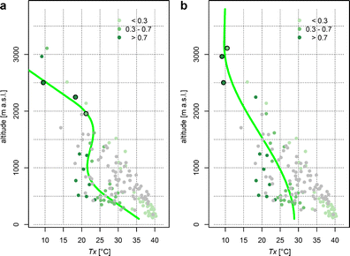
Vertical profile for subregion northwest on a day with a strong west–east temperature gradient (Tx, 08.08.2013), points for station observations, lines for the fitted profile. Subregional weighting of stations is depicted by colour strength (see inset). Cold-pool stations omitted from profile fitting are shown as grey dots. Summit stations selected to estimate the linear lapse rate γ are marked by circled dots. a. Arbitrary selection of summit stations for lapse rate estimation. b. Progressive selection of summit stations for lapse rate estimation
-
Generalised distance fields: Applying the interpolation method over a larger region, with a denser grid spacing and with more stations introduced substantially higher computational costs in the derivation of the generalised distance fields (note that these calculations are needed only once and prior to the actual interpolation). To limit computation times, the domain, over which the generalised distance fields are calculated, was confined to a square area of 200 × 200 km. The map sections shown in Fig. 3 depict the results over these computation domains (Frei (2014) was calculating these fields over the entire domain). This adaptation is purely technical. It does not constrain the number of stations available for any target grid point beyond other imposed constraints. Similarly to the original application (Frei 2014), the four closest stations are used for residual weighting. This choice provides a reasonable compromise between resolution of regional detail and robustness of interpolation.
-
Set of layering coefficient: In contrast to the original application, where the residual weighting (employed layering coefficient λ) is selected on a day-by-day basis, we decided for a constant of λ = 100 for all cases. This decision is motivated by the frequency distribution of λ-values obtained with the original flexible λ-procedure (Fig. 5). For both Tn and Tx, there seems to be a strong topographic influence (λ = 100) in the residual patterns for most of the days. Closer inspection of cases when the flexible procedure decided for a low value of λ (e.g. between 0 and 30) revealed that many of them were more plausibly interpolated with a higher λ instead. This happened because conditions over the large lowland areas of Austria are overrepresented. As a result, strong topographic residual signals, e.g. from night-time cooling or day-time heating in Alpine valleys, were, in some cases, dominated by the flatland conditions. For this reason, we decided to disable the feature of a flexible distance metric and to impose a fixed value of λ = 100 throughout. It resolves the described problem, but no adverse effects were evident in other cases. Frei (2014) showed that the difference in cross-validation error between using a variable or a constant setting of λ was very small in Switzerland (see his Fig. 13).
Fig. 5 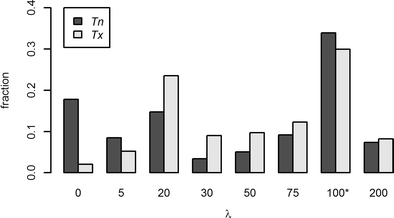
Histogram of layering coefficients λ, which the method would choose when a flexible (data driven) choice of λ would be allowed. Histograms are displayed for Tn and Tx and were obtained from an experiment over all days of 2011 and 2012. For the final gridded dataset, a fixed value of λ = 100 (marked with asterisk) was applied in all cases
-
Urban heat island: Due to the usage of inner-city stations and a high spatial resolution, we decided to model the urban heat island effect in the interpolation. This should also avoid confusion of urban thermal anomalies with topographic patterns. An urban thermal pattern was estimated from the inner-city stations of the three largest Austrian cities, namely Vienna, Graz and Linz. Firstly, the urban area was identified out of the Austrian CORINE Land Cover model (Umweltbundesamt 2014). Secondly, the grid points within the urban area were subjectively distance-weighted with values between 0 at the location of the inner-city station and 10 at the city’s edge. This procedure is motivated by urban climatologies (Auer et al. 1989) and results from modelling studies on urban climate (Žuvela-Aloise et al. 2014). Thirdly, the regularly calculated generalised distance field of the inner-city station was gradually upscaled to a new minimum of 50 (scaled) km. Finally, the urban representativity field of step 2 and the rescaled generalised distance field of step 3 were superimposed. The resulting modified generalised distance field for the inner-city station of Vienna is depicted in Fig. 3d. Even if urban effects may be present in smaller cities as well (cf. Wienert et al. 2013), these are not estimated here due to the lack of corresponding inner-city observations.


4 Results
After implementation and adaptation, the interpolation method was processed over the entire study period. The final dataset consists of more than 38,000 daily Tn- and Tx-fields starting in 1961. In addition to these original grids, aggregates at a monthly, seasonal and annual time resolution were produced. The grids were also used to calculate anomalies with respect to the long-term mean of the reference period 1961–1990, again at daily, monthly, seasonal and annual resolutions. Altogether, the data product encompasses about 61,000 fields. In internal project and product administration, the presented dataset is referred to as SPARTACUS (spatiotemporal reanalysis dataset for climate in Austria).
The following subsections summarise results from a detailed visual inspection (Section 4.1) and from a systematic evaluation of the procedures by means of cross-validation (Section 4.2). We then compare several examples of the newly produced temperature dataset against existing datasets in Austria (Section 4.3). Was the quality of this new analysis compromised by the constraint to fewer, yet complete station series? If so, this may be visible in a lack of spatial detail compared to datasets that have exploited more (all) available information. In the final Subsection 4.4, we test how well the interpolation can reproduce long-term trends and provide example results from its application in quantifying long-term trends in impact-related climate indices.
4.1 Example
Extensive visual inspections of the temperature fields for variable weather conditions were conducted to obtain confidence in the overall performance of the employed methods. One such example case is shown in Fig. 6. The figure depicts results from all major interpolation steps for the construction of the Tn field on a winter day with marked valley-scale cold-pools. The upper panels (Fig. 6a) show the estimation of the three nonlinear subregional vertical profiles on basis of the weighted station measurements. It should be noted that the temperature profiles are representative at a larger scale (background field) and, hence, they do not replicate the cold conditions met at stations in Alpine valleys. Valley stations prone to cold-pools are discarded from the estimation of the background field anyway. In subregion south, which includes the Klagenfurt and Graz basins, a moderate inversion layer is visible both in the station data and the fitted profile. Together, the three subregion profiles define the background field. Residuals at stations from this background field are occasionally quite large (exceeding 8 °C for several stations, Fig. 6b). These are stations in Alpine valleys, obviously affected by the formation of a valley-scale cold-pool. Note that magnitude of the residuals varies between different valleys and that only small, mainly positive residuals are found over the foreland regions. The residual interpolation plausibly distributes these anomalies (Fig. 6b). It extends cold-pool residuals along the valley axes and even penetrates them into nearby tributaries. The non-Euclidean distance weighting scheme is crucial for this distribution. Indeed, if these residuals would have been interpolated with a Euclidean distance weighting instead, the cross-validation error (over all stations) would have been 20 % larger. The final temperature interpolation is shown in Fig. 6c. It is the result from superimposing the background and the residual fields. A complex temperature pattern emerges, with differently cold Alpine valleys and basins (−15 to −2 °C), temperate mid- and high-altitudes (−10 to 0 °C), a cold Graz basin (around −6 °C) and rather mild conditions in the Rhine valley and in the northern Alpine foreland (−2 to 6 °C) peaking in the city centre of Vienna (7 °C). There is a good correspondence with the in situ observations, lending credibility to the inferred temperature field.

Illustration of the calculation steps and intermediate results obtained for the analysis of Tn on 05.01.1992. a. Profiles: Vertical profiles for subregions northwest, northeast and south, points for station observations, lines for the fitted profile. Subregional weighting of stations is depicted by colour strength (see inset). Cold-pool stations omitted from profile fitting are shown as grey dots. Summit stations selected to estimate the linear lapse rate at high elevations are marked by circles. b. Residuals: Station residuals (colour-filled circles) and interpolated residual field (in °C). c. Analysis: Station observations (colour-filled circles) and resulting Tn field (in °C)
Investigation of several other meteorological situations revealed that the method is capable of producing plausible temperature fields. Cases studied include situations with almost linear altitude-temperature relationship, basin-scale inversions over the foreland regions, föhn and strong horizontal gradients. Frei (2014) has illustrated the working of the adopted interpolation scheme for several such cases in Switzerland (see his Figs. 7, 8 and 9) and we therefore renounce here from depicting additional examples from Austria.
4.2 Systematic evaluation
For the purpose of a quantitative assessment of the interpolation errors, we have conducted a systematic cross-validation by omitting each of the 150 stations in turn. The validation was conducted for the 10 years from 2003 to 2012. We start by considering error metrics averaged over the 112 stations within Austrian borders, both for Tn and Tx (Table 1). The compound mean error (ME, error averaged over time and space) measures overall bias. It is very close to 0 °C, indicating that there is no systematic under- or overestimation (bias) of temperature by the interpolation method. The mean absolute error (MAE), again averaged over time and space, is 1.1 and 1.0 °C for Tn and Tx, respectively. The root-mean-square error (RMSE) is around 1.4 °C. Further validation (not shown) over the entire study period and with a small sample of test stations indicates that the error statistics tend to gradually decrease over the study period. But these trends are small compared to the absolute value (less than 10 % change), which implies that the error figures reported here can be considered representative for the entire period.
Figure 7 depicts maps of the station-wise error measures ME and MAE for both Tn and Tx. It reveals that there is a tendency to overestimate Tn at locations prone to cold-pool formation (Fig. 7a). The bias is around 0.5–2.5 °C and indicates that the intensity of valley-scale cold anomalies is underestimated by the method in valleys without a station observation. Conversely, inner-city stations are subject to a slight systematic underestimation of Tn, again suggesting an underestimation of urban warm anomalies when stations are omitted. Comparing ME values between Tn and Tx reveals that the range of ME values is considerably smaller for Tx (Fig. 7b). Tx is overestimated at summit stations, possibly due to an underestimation of boundary-layer effects in the vertical profiles. Similar maps for the random errors (MAE, Figs. 7c, d) show that the largest MAE values are met at stations outside of Austria. This is not surprising considering their larger distance to neighbours and it justifies the effort made in this study to include foreign stations in the analysis. Without this, the degraded performance would probably have been imported to the core study region. Within the country, larger MAE are typically found for cold-pool stations in case of Tn and at summit stations in case of Tx. Note that random errors at such sites can be as large as 1.5–3 °C, whereas they are frequently below 1 °C at less exposed sites.

Error measures from leave-one-out cross-validation for individual stations. Shown are mean error (ME, bias, in °C) and mean absolute error (MAE, in °C) for minimum (Tn) and maximum (Tx) temperature. Downward triangles mark stations at locations prone to cold-pool formation, upward triangles stations at summit locations, diamonds stations at inner-city locations and circles stations at all other locations. Values are averaged over the years from 2003 to 2012, for which the cross-validation was conducted
Figure 8 depicts the annual course of the MAE stratified by five geographical subentities of Austria. Considering Tn (Fig. 8a), both inner-Alpine valley and summit stations exhibit a weak seasonal course with higher error values in late autumn and winter and lower error values in summer. This is likely related to the seasonal frequency and intensity of valley-scale cold-pools. Stations in the Bohemian Massif and, to some extent, also in the northern foreland exhibit two annual maxima in MAE in spring and autumn. The reason for this behaviour is not entirely clear. Possibly, the spatial variance of temperatures is relatively larger in these periods, as a result of larger dynamic activity and the frequent occurrence of föhn.

Annual course of the mean absolute error (MAE, in °C) averaged over stations in geographical subentities for Tn (a) and Tx (b). Values are averaged over the years from 2003 to 2012, for which the cross-validation was conducted. Results include within-Austria stations only
For Tx (Fig. 8b), there is much smaller variation of MAE values over the year in all regions, except for inner-Alpine valley stations. MAE peaks in December or January in all lowland regions inside and outside of the Alps. However, the figure reveals the consistently higher error level at summit stations, which in part may be related to biases from the extrapolation of boundary-layer conditions from lower levels, but it is certainly also due to the fact that stations at similar altitude are usually much more distant for summit than for low-level stations.
Due to different topographical and climatological conditions, observational input data, network densities and test procedures, it is difficult to compare error metrics between different spatial interpolation datasets reported in the literature. At this point, it is, nevertheless, worth mentioning that the cross-validation errors found with the presented interpolation in Austria are similar compared to those reported for other interpolation procedures, which are based on a larger number of input stations. The MAE values of Tn and Tx in this study are slightly lower compared to those listed in Hasenauer et al. (2003) for the Daymet interpolation applied over Austria. Moreover, MAE values are approximately the same like those obtained with the numerical weather model-based analysis system INCA (however, for hourly temperature there; Haiden et al. 2011). In its original application in Switzerland, the interpolation method produces even about 10 % smaller errors compared to Austria. The difference between the Swiss and the Austrian applications can be explained by the following facts: The statistics reported in Frei (2014) for Switzerland refer to daily mean temperature. Minimum and maximum temperatures, considered in this study, are subject to higher variability, expose more complex and less structured relationships to topography and are susceptible to larger measurement errors. Furthermore, the Swiss application relies on a denser station network, using 1 station per 375–590 km2 compared to 1 station per 749 km2 in Austria.
4.3 Qualitative comparison with other gridded datasets
For the presented grid dataset, we have chosen to utilise observational time series only that have an almost complete coverage over the study period. The restriction is meant to improve consistency in sampling conditions over time, which is essential when using the dataset for climate monitoring, such as for the identification of long-term trends. Evidently, there is a compromise incurred. The approach does not exploit the full volume of observational information at any particular instant, which may affect plausibility and accuracy of the resulting interpolation.
In this subsection, we illustrate that the volume of available station observations utilised in our interpolation, although reduced, renders temperature patterns that are at least similarly realistic compared to existing temperature datasets over Austria, generated with other interpolation methods and, eventually, incorporating more station data. Grids from the present dataset (SPARTACUS), which is based on 150 station observations, are compared against grids of daily temperature from INCA (about 550 stations), against Daymet (between 192 and 285 stations, depending on year) and against StartClim datasets (about 70 stations) (see Section 1.1 for a short description of the datasets). Note that some differences between analyses may also be due to differences in the underlying DEM (only minor effect here) and between analysed parameters (Tm in StartClim).
-
Inner-Alpine valley-scale inversions (Tn, 14.01.2006): Reproduction of small-scale cold-pools in individual valleys and basins requires a high degree of spatial differentiation. Figure 9a compares results for such a case between the INCA grid and the SPARTACUS grid. In INCA, the cold-pools are evident as locally confined cold spots and warm upper-level conditions as warm anomalies around single summit stations. In the SPARTACUS dataset, the temperature distribution appears considerably more stratified. Cold-pool-affected valleys and basins are completely filled with cold anomalies and warm conditions at higher altitudes are spatially more extended than in INCA. In Daymet (not shown), the same case exhibits a rather implausible temperature distribution with strong horizontal gradients across mountains and valleys. With a much smaller number of stations, StartClim (not shown) accomplishes a more topography-bound spatial distribution in this particular case.
Fig. 9 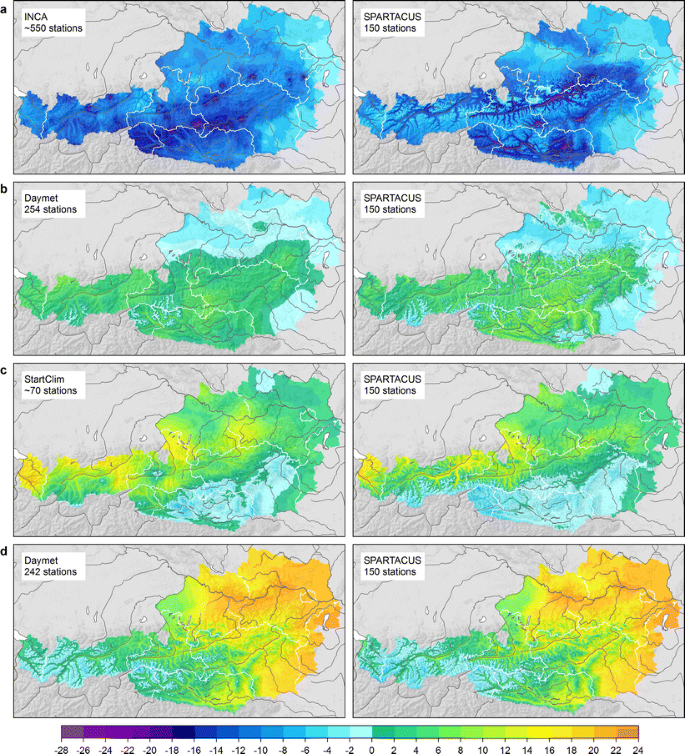
Comparison of temperature analyses in Austria as derived by SPARTACUS and several existing gridded datasets (in °C). The depicted cases represent conditions with temperature patterns that are challenging for spatial analysis. a Inner-Alpine valley-scale inversions, Tn on 14.01.2006. b Extra-Alpine basin-scale inversions, Tx on 31.01.2006. c Föhn, Tm (SPARTACUS: (Tn + Tx) / 2 for comparability) on 08.11.1982. d Strong horizontal gradients, Tx on 06.04.1975
-
Extra-Alpine basin-scale inversions (Tx, 31.01.2006): On this day, all four gridding products consistently show an extensive shallow inversion layer over the northern and eastern forelands (related to low stratus) and warm mid-altitudes (related to mainly clear sky conditions). A visual comparison of the Daymet and SPARTACUS grids is depicted in Fig. 9b. Like in the previous case, INCA (not shown) exhibits a pattern with localised cold and warm anomalies within the Alps, centred at station locations. Such a pattern can also be seen in Daymet, but with much smoother horizontal gradients. Several important spatial anomalies are poorly structured or missing, such as the warm anomaly in the uplands of the Bohemian Massif or the cold anomaly in the Klagenfurt basin. The SPARTACUS grid shows a topographically strongly structured temperature distribution. Frosty areas at the northern fringe of the Alps penetrate from the forelands into the valleys. This pattern seems unlikely in view of additional station observations that day. However, both INCA and Daymet miss much of the spatial detail, although the station data utilised is considerably denser than in SPARTACUS.
-
Föhn (Tm, 08.11.1982): The temperature distributions for this day are very similar for INCA, Daymet and SPARTACUS. There are warm anomalies in northbound Alpine valleys and along the northern fringes of the ridge, a pattern characteristic for föhn. Figure 9c depicts the StartClim and SPARTACUS grids. Although the StartClim grid resembles the overall pattern and range of temperature in SPARTACUS, it expands positive anomalies across mountain ranges. Also, it seems to contain implausible features like the cold anomaly in western Salzburg and the warm anomaly in western Lower Austria, which are not supported by additional station observations. High altitudes are generally warmer in the StartClim grid compared to SPARTACUS. It seems that StartClim is suffering from the constrained observational input in weather situations with pronounced topographic effects.
-
Strong horizontal gradients (Tx, 06.04.1975): Situations with strong horizontal gradients, for example related to a front’s westward passage, are usually captured well by all four spatial datasets. The Daymet and the SPARTACUS grids are depicted in Fig. 9d. Daymet and StartClim (not shown) picture a noticeable west-to-east temperature gradient in Upper Austria on this day. This is also evident in SPARTACUS, but here the contrasts are also evident within the ridge. The known phenomenon that warmer air lasts somewhat longer, possibly supported by föhn effects as well, in inner-Alpine valleys (like the Upper Salzach and Upper Enns Valleys in this situation) becomes apparent in the SPARTACUS grid.

4.4 Analysis of long-term trends
In the construction of the present gridded dataset, a particular effort was made to avoid temporal inconsistencies due to variations in the station network and, hence, to permit for a more robust analysis of long-term trends than is currently possible with existing grid datasets for Austria. Later in this subsection, we will illustrate this application by depicting long-term trends for several temperature-based climate indices, derived from SPARTACUS. Adequate interpretation of such trend results shall, however, be guided by knowledge about the reliability of long-term trends inferred from a grid dataset. Magnitude and spatial pattern of trends may be affected by interpolation errors and remaining inhomogeneities (which have not or insufficiently been removed by the correction procedures) in the utilised station time series. Our discussion of trend results shall therefore be preceded by an estimation of trend errors to be expected in the gridded dataset for locations (grid points) without direct observation.
The assessment of trend accuracy builds on a leave-one-out cross-validation conducted for all 112 stations within Austria, day-by-day over the entire period from 1961 to 2013. The results are independent time series of temperature estimates as predicted by the interpolation method, just like for an ungauged site. Comparison of the long-term trends between the predicted and the observed daily series yields estimates of trend errors that have to be expected when calculating trends from the grid dataset grid point by grid point.
Figure 10 depicts scatterplots of the observed and predicted trends, each point representing the results for one of the stations. Results are shown for the trend in mean annual temperature estimated by linear regression (Fig. 10a) and for the trend in the annual number of freeze-thaw days (Tn < 0 °C and Tx > 0 °C, Fig. 10b). In the latter case, trends were determined by logistic regression and are expressed as odds ratio (e.g. Frei and Schär 2001). In the case of rare occurrence, the odds ratio is approximately equal to the ratio of annual freeze-thaw days between the end and the beginning of the period. Odds ratios smaller (larger) than 1 indicate a decrease (increase) over time.

Scatterplots of observed trends versus predicted trends as estimated by the interpolation method from a leave-one-out cross-validation. Shown are linear trends of the annual mean of air temperature (mean of Tn and Tx, a) and odds ratios from a logistic trend analysis of the annual sum of freeze-thaw-days (b) over the period 1961–2013. Results from station series (partly) homogenised on a daily basis are shown in green, those from all other stations in black
The results reveal that there is correspondence between predicted and observed trends in that there is a positive correlation between the two. In the case of mean annual temperature (Fig. 10a), differences between estimated and observed trend are mostly smaller than 0.1 °C per 10 years and, hence, trend errors are clearly smaller than the average trend over the region. However, the spatial variation of the trend (observed) is smaller than the average trend and, hence, the magnitude of trend errors can influence the spatial pattern. The best linear fit between predicted and observed trends has a slope smaller than 1, indicating that the spatial contrast of trends is underestimated by the gridded dataset, likely an effect of the smoothing inherent to spatial interpolation. Closer inspection revealed that many stations where the observed trend was overestimated are inner-Alpine valley stations, prone for valley-scale cold-pools. Also, many outliers in the scatterplot could be attributed to stations that experienced major relocations, i.e., the observed trend may be affected by residual inhomogeneity. Good agreement between predicted and observed trends in annual mean temperature was found for the high-Alpine summit stations. The present analysis suggests that interpolation errors (and residual inhomogeneities) indeed pose a certain limitation on the accuracy, with which the SPARTACUS grid dataset can represent details in the spatial pattern of long-term trends. Nevertheless, the Pearson correlation of 0.53 also suggests that major spatial contrasts are qualitatively trustworthy. It is interesting to compare this with results from a similar cross-validation exercise conducted for Switzerland (Frei 2014). Despite a slightly denser station network, the correlation was only 0.12 and there were instances with much larger trend errors (see Fig. 15 in Frei 2014). However, the station network utilised for the interpolation in Switzerland varies over time. The better correspondence found here suggests that the accuracy of spatial trend mapping has indeed benefited from reducing variations in the station network.
The results of a similar assessment of trend accuracy for freeze-thaw days (Fig. 10b) are qualitatively similar to those for mean temperature, i.e. good agreement in trend magnitude but restricted correspondence in spatial patterns (Pearson correlation 0.41). Again, the spatial contrasts in the predictions are smaller than those in the observations, likely due to smoothing. The case of trends in freeze-thaw days is challenging, because threshold-based climate indices (counts) are particularly sensitive to interpolation errors and temporal inhomogeneities when the threshold is at the tail of the distribution (Katz and Brown 1992). Indeed, there are a few individual stations, for which the correspondence is particularly poor and these have a strong effect on the correlation coefficient.
The distinction between conventional series and series homogenised on a daily basis (black and green symbols in Fig. 10) does not indicate a clear difference between them. For trends in air temperature, the interpolation at locations with homogenised series performs better in terms of correlation, but the opposite is true for trends in freeze-thaw days. One could have expected that the different data quality level between the two groups may become apparent in the comparison with predicted series, however, it seems that other influences, like site peculiarities and interpolation errors, have a large influence too.
Our assessment suggests that the daily SPARTACUS dataset can reasonably represent the typical magnitude of trends in climate indices over Austria. It may also reproduce the major spatial pattern of trends qualitatively, but spatial contrasts are likely underestimated and more regional features may be distorted by interpolation errors. Particular caution is required in the interpretation of trend results for inner-Alpine valleys when these are not explicitly sampled in the station network.
Bearing these precautions in mind, we turn to illustrate the utility of the SPARTACUS dataset for climate monitoring and climate impact research by analysing trends for three selected climate indices and, hence, exploiting the daily time resolution available with this new dataset. All three indices are counts of days per year. To be consistent with the discrete nature of count data, our analysis builds on logistic regression with maximum likelyhood estimation, a 5 % significance level and correction for overdispersion when testing against the null hypothesis “no trend” (see Frei and Schär 2001 for details). The trend magnitude is expressed as odds ratio over the 53-year period 1961–2013 (Fig. 11).

Trend in three temperature-based climate indices, derived from the daily SPARTACUS dataset over the 53-year period 1961–2013. The trend magnitude (in colour) is expressed as odds ratio estimated from logistic regression of the annual counts. Hatching denotes areas where trends are significant at the 5 % level. a Freeze-thaw days. b Cold spell duration index. c Bark beetle activity period
-
Freeze-thaw days: The annual number of days, on which temperature passes the freezing point, is an indicator for the climatic exposure of constructions and the stability of permafrost areas. In most regions of Austria, there is a clear decrease in the odds of the occurrence of freeze-thaw days over the period 1961–2013 (Fig. 11a). The largest decreases are found in the Lower Inn Valley and generally north of the Alps. In these areas, the trend is statistically significant. In contrast, the frequency of freeze-thaw days remained widely unchanged in high-Alpine regions and also in the Klagenfurt basin and parts of the Graz basin. Increases are found in few well-known cold-pool locations. However, these are not statistically significant. Both decreases and increases are plausibly explained by a general shift towards higher temperatures.
-
Cold spell duration index: The annual count of days, which are part of an outstandingly cold episode (at least 6 days where Tn is below the calendar day’s 10th percentile), has been calculated accordingly to Klein Tank et al. (2009). The occurrence of days within a cold spell has decreased almost everywhere in Austria during the 53-year period (Fig. 11b). Apparently, there is a horizontal gradient from small changes in the eastern part of the country towards significant decreases in the northwest of Austria. Strong decreases are also found in the Rhine valley, the Lower Inn Valley and at low altitudes in southern Austria.
-
Bark beetle activity period: Outbreaks of bark beetles are forest-damaging and can entail serious ecological and economical consequences. The calculation of the annual duration of the insect’s activity period involves a threshold check (Tx > 20 °C) and the definition of core and partial periods (similar to common definitions of vegetation period). The period of activity became significantly longer over most parts of Austria over the years from 1961 to 2013 (Fig. 11c). In large parts of the northern Alpine foreland, in the Inn Valley and at the edge of the Graz basin, the frequency of days within an activity period increased by up to three times and more.
5 Conclusions
This paper presents the methodology and example analyses of a new spatial dataset of daily minimum and maximum temperature covering the territory of Austria with a resolution of 1 km and extending over a period of more than 53 years starting in 1961. While several temperature datasets already exist for this region, our development was guided by two specific advancements. Firstly, weather in the Alpine region is frequently accompanied by complex and nontrivial temperature distributions and this calls for an interpolation method dedicated to complex terrain. Secondly, actual interest of many users into temperature variations and trends calls for particular attention into long-term consistency and this meant to account for difficulties arising with the changes in observational coverage (station density) and measurement inhomogeneities.
As for the first requirement, we chose a recently developed interpolation method (Frei 2014) that deals explicitly with common nonlinearities in the vertical temperature structure and with topographical imprints in the spatial representativity of station observations. Several adaptations of the method were necessary to cope with peculiarities of the physiography and station distribution in Austria. Notably, the number of subdomains was increased, the estimation of vertical profiles improved and a module for urban heat island effects was integrated. Several example cases suggest that there is a clear benefit from the more versatile interpolation method. Especially during challenging weather conditions (valley-scale inversions and föhn), the results turned out to be more plausible (at least not inferior) than those found in existing datasets, even though the latter eventually use more station observations.
As for the long-term consistency, we chose to run the interpolation with data from a time-invariant station network. The common principle to use all observational information when it is available was abandoned to avoid inhomogeneities in sampling conditions that bear on interpolation error statistics and ultimately compromise the long-term consistency of the dataset. To sidestep excessive loss of utilisable data, time series with a short missing period were complemented with a standalone gap-filling procedure. Homogenised daily station data were utilised when they were available. For stations that were not (yet) subjected formally to a daily homogenisation, more ad hoc corrections were made for known station relocations in altitude and known inhomogeneities in the monthly time series. Cross-validation experiments support the role of these efforts for improving long-term consistency, but the resulting dataset is not entirely free of inhomogeneities. Future improvements of the dataset will therefore focus on the homogenisation of the full input dataset (Tn and Tx series) at the daily time scale.
Leave-one-out cross-validation reveals that the interpolation error (mean absolute error averaged over all stations) is 1.1 °C for daily minimum and 1.0 °C for maximum temperature. Larger errors must be expected in the gridded dataset for unsampled inner-Alpine valleys, where minimum temperatures tend to be systematically overestimated and random errors are larger, notably during episodes with valley-scale cold-pools. Error measures found in our tests are comparable to similar measures reported for already existing gridded temperature datasets for Austria. Comparability of these error measures is limited, given the differences in test samples, but visual comparisons also suggest that the present dataset improves particularly in situations with complex mesoscale temperature distributions like valley-scale inversions and föhn. Furthermore, the method’s tendency to vertically constrain temperature anomalies appears as an evident advantage in the comparisons. It is noteworthy that the present interpolation method utilises observations and a digital elevation model only, but its results are qualitatively similarly plausible like those of a comprehensive analysis (INCA) with a numerical weather forecasting model and many more station observations.
A key novelty of the present dataset is the combination of daily time resolution, coverage of minimum and maximum temperatures and multidecadal extent. This opens a wide range of possible applications, concerned with the long-term variation of temperatures over the past decades. Operational climate monitoring, climate change detection, the evaluation of climate models and climate services for resources planning and natural hazard protection are example areas where this dataset can be adopted. It may also advance climate impact research in many disciplines (agronomy, forestry, hydrology, glaciology, pedology, etc.), because it describes the climatic conditions that have accompanied changes in many natural systems over the past decades. Several of these systems involve nonlinear dependencies on temperature. The daily time resolution of the present dataset permits for their explicit modelling or for simplified quantifications through dedicated impact indices. A set of preliminary analysis in this study suggests that Austria experienced significant changes in impact-related thermal conditions over the past 50 years.
The SPARTACUS dataset comprises, at present, around 61,000 grids and is operationally updated on a daily basis to facilitate operational climate monitoring applications. The dataset is available from ZAMG for scientific applications in climate (impact) research, official planning and hazard management. It is envisaged to complement this temperature dataset with similar daily gridded datasets for other climate parameters like precipitation and sunshine duration.
Change history
05 November 2022
A Correction to this paper has been published: https://doi.org/10.1007/s00704-022-04250-x
References
Auer I, Böhm R, Mohnl H (1989) Klima von Wien. Eine anwendungsorientierte Klimatographie. Magistrat der Stadt Wien, Vienna
Auer I, Böhm R, Jurkovic A, Lipa W, Orlik A, Potzmann R, Schöner W, Ungersböck M, Matulla C, Briffa K, Jones PD, Efthymiadis D, Brunetti M, Nanni T, Maugeri M, Mercalli L, Mestre O, Moisselin JM, Begert M, Müller-Westermeier G, Kveton V, Bochnicek O, Stastny P, Lapin M, Szalai S, Szentimrey T, Cegnar T, Dolinar M, Gajic-Capka M, Zaninovic K, Majstorovic Z, Nieplova E (2007) HISTALP—historical instrumental climatological surface time series of the Greater Alpine Region 1760–2003. Int J Climatol 27:17–46. doi:10.1002/joc.1377
Bénichou P, Le Breton O (1987) Prise en compte de la topographie pour la cartographie des champs pluviométrique. La Météorologie 7:23–34
Bica B, Steinacker R, Lotteraner C, Suklitsch M (2007) A new concept for high resolution temperature analysis over complex terrain. Theor Appl Climatol 90:173–183. doi:10.1007/s00704-006-0280-2
Bukovsky MS, Karoly DJ (2007) A brief evaluation of precipitation from the North American regional reanalysis. J Hydrometeorol 8:837–846. doi:10.1175/JHM595.1
Caussinus H, Mestre O (2004) Detection and correction of artificial shifts in climate series. J R Stat Soc Ser C Appl Stat 53:405–425. doi:10.1111/j.1467-9876.2004.05155.x
Chimani B, Matulla C, Böhm R, Hofstätter M (2013) A new high resolution absolute temperature grid for the Greater Alpine Region back to 1780. Int J Climatol 33:2129–2141. doi:10.1002/joc.3574
Daly C, Neilson RP, Phillips DL (1994) A statistical-topographical model for mapping climatological precipitation over mountainous terrain. J Appl Meteorol 33:140–158. doi:10.1175/1520-0450(1994)033<0140:ASTMFM>2.0.CO;2
Daly C, Halbleib M, Smith JI, Gibson WP, Doggett MK, Taylor GH, Curtis J, Pasteris PP (2008) Physiographically sensitive mapping of climatological temperature and precipitation across the conterminous United States. Int J Climatol 28:2031–2064. doi:10.1002/joc.1688
Donat MG, Alexander LV, Yang H, Durre I, Vose R, Dunn RJH, Willett KM, Aguilar E, Brunet M, Caesar J, Hewitson B, Jack C, Klein Tank AMG, Kruger AC, Marengo J, Peterson TC, Renom M, Oria Rojas C, Rusticucci M, Salinger J, Elrayah AS, Sekele SS, Srivastava AK, Trewin B, Villarroel C, Vincent LA, Zhai P, Zhang X, Kitching S (2013) Updated analyses of temperature and precipitation extreme indices since the beginning of the twentieth century: the HadEX2 dataset. J Geophys Res Atmos 118:2098–2118. doi:10.1002/jgrd.50150
Frei C (2014) Interpolation of temperature in a mountainous region using nonlinear profiles and non-Euclidean distances. Int J Climatol 34:1585–1605. doi:10.1002/joc.3786
Frei C, Schär C (2001) Detection probability of trends in rare events: theory and application to heavy precipitation in the Alpine region. J Clim 14:1564–1584. doi:10.1175/1520-0442(2001)014<1568:DPOTIR>2.0.CO;2
Haiden T, Kann A, Wittmann C, Pistotnik G, Bica B, Gruber C (2011) The integrated nowcasting through comprehensive analysis (INCA) system and its validation over the Eastern Alpine Region. Weather Forecast 26:166–183. doi:10.1175/2010WAF2222451.1
Hasenauer H, Merganicova K, Petritsch R, Pietscha SA, Thornton PE (2003) Validating daily climate interpolations over complex terrain in Austria. Agric For Meteorol 119:87–107. doi:10.1016/S0168-1923(03)00114-X
Haslinger K, Anders I, Hofstätter M (2013) Regional climate modelling over complex terrain: an evaluation study of COSMO-CLM hindcast model runs for the Greater Alpine Region. Clim Dyn 40:511–529. doi:10.1007/s00382-012-1452-7
Haslinger K, Koffler D, Schöner W, Laaha G (2014) Exploring the link between meteorological drought and streamflow: effects of climate-catchment interaction. Water Resour Res 50:2468–2487. doi:10.1002/2013WR015051
Hiebl J, Auer I, Böhm R, Schöner W, Maugeri M, Lentini G, Spinoni J, Brunetti M, Nanni T, Perčec-Tadić M, Bihari Z, Dolinar M, Müller-Westermeier G (2009) A high-resolution 1961–1990 monthly temperature climatology for the greater Alpine region. Meteorol Z 18:507–530. doi:10.1127/0941-2948/2009/0403
Huss M, Farinotti D, Bauder A, Funk M (2008) Modelling runoff from highly glacierized alpine drainage basins in a changing climate. Hydrol Process 22:3888–3902. doi:10.1002/hyp.7055
Isotta FA, Vogel R, Frei C (2014) Evaluation of European regional reanalyses and downscalings for precipitation in the Alpine region. Meteorol Z. doi:10.1127/metz72014/0584
Kapeller S, Lexer MJ, Geburek T, Hiebl J, Schueler S (2012) Intraspecific variation in climate response of Norway spruce in the eastern Alpine range: selecting appropriate provenances for future climate. For Ecol Manag 271:46–57. doi:10.1016/j.foreco.2012.01.039
Katz RW, Brown BG (1992) Extreme events in a changing climate: variability is more important than averages. Clim Chang 21:289–302. doi:10.1007/BF00139728
Klein Tank AMG, Zwiers FW, Zhang X (2009) Guidelines on analysis of extremes in a changing climate in support of informed decisions for adaptation. World Meteorol Organ. http://eca.knmi.nl/documents/WCDMP_72_TD_1500_en_1.pdf. Accessed 18 Sept 2014
Luhamaa A, Kimmel K, Männik A, Rõõm R (2011) High resolution re-analysis for the Baltic Sea region during 1965–2005 period. Clim Dyn 36:727–738. doi:10.1007/s00382-010-0842-y
Massmann C, Holzmann H (2012) Analysis of the behavior of a rainfall-runoff model using three global sensitivity analysis methods evaluated at different temporal scales. J Hydrol 475:97–110. doi:10.1016/j.jhydrol.2012.09.026
Masson D, Frei C (2014) Long-term variations and trends of mesoscale precipitation in the Alps: Recalculation and update for 1901–2008. Int J Climatol (submitted)
Mestre O, Gruber C, Prieur C, Caussinus H, Jourdain S (2011) SPLIDHOM, a method for homogenization of daily temperature observations. J Appl Meteorol Climatol 50:2343–2358. doi:10.1175/2011JAMC2641.1
Nemec J, Gruber C, Chimani B, Auer I (2013) Trends in extreme temperature indices in Austria based on a new homogenised dataset. Int J Climatol 33:1538–1550. doi:10.1002/joc.3532
Olefs M, Schöner W, Suklitsch M, Wittmann C, Niedermoser B, Neururer A, Wurzer A (2013) SNOWGRID—a new operational snow cover model in Austria. International Snow Science Workshop Proceedings 2013:38–45. http://arc.lib.montana.edu/snow-science/item/1785. Accessed 18 Sept 2014
Petritsch R, Hasenauer H (2014) Climate input parameters for real-time online risk assessment. Nat Hazards 70:1749–1762. doi:10.1007/s11069-011-9880-y
R Core Team (2011) R: a language and environment for statistical computing. R Foundation for Statistical Computing, Vienna. ISBN: 3-900051-07-0. http://www.R-project.org. Accessed 18 Sept 2014
Rienecker MM, Suarez MJ, Gelaro R, Todling R, Bacmeister J, Liu E, Bosilovich MG, Schubert SD, Takacs L, Kim GK, Bloom S, Chen J, Collins D, Conaty A, da Silva A, Gu W, Joiner J, Koster RD, Lucchesi R, Molod A, Owens T, Pawson S, Pegion P, Redder CR, Reichle R, Robertson FR, Ruddick AG, Sienkiewicz M, Woollen J (2011) MERRA: NASA’s modern-era retrospective analysis for research and applications. J Clim 24:3624–3648. doi:10.1175/JCLI-D-11-00015.1
Ruefenacht B, Finco MV, Nelson MD, Czaplewski R, Helmer EH, Blackard JA, Holden GR, Lister AJ, Salajanu D, Weyermann D, Winterberger K (2008) Conterminous U.S. and Alaska forest type mapping using forest inventory and analysis data. Photogramm Eng Remote Sens 74:1379–1388
Schöner W, Dos Santos Cardoso E (2004) Datenbereitstellung, Entwicklung von Regionalisierungstools und einer Schnittstelle zu den regionalen Klimamodellen. Zentralanstalt für Meteorologie und Geodynamik. http://foresight.ait.ac.at/SE/projects/reclip/reports/report6_Regionalisierung_ZAMG.pdf. Accessed 18 Sept 2014
Seidl R, Schelhaas MJ, Lindner M, Lexer MJ (2009) Modelling bark beetle disturbances in a large scale forest scenario model to assess climate change impacts and evaluate adaptive management strategies. Reg Environ Chang 9:101–119. doi:10.1007/s10113-008-0068-2
Steinacker R, Ratheiser M, Bica B, Chimani B, Dorninger M, Gepp W, Lotteraner C, Schneider S, Tschannett S (2006) A mesoscale data analysis and downscaling method over complex terrain. Mon Weather Rev 134:2758–2771. doi:10.1175/MWR3196.1
Steinacker R, Mayer D, Steiner A (2011) Data quality control based on self-consistency. Mon Weather Rev 139:3974–3991. doi:10.1175/MWR-D-10-05024.1
Szentimrey T, Bihari Z, Lakatos M, Szalai S (2011) Mathematical, methodological questions concerning the spatial interpolation of climate elements. Időjárás 115:1–11
Themeßl MJ, Gobiet A, Leuprecht A (2011) Empirical-statistical downscaling and error correction of daily precipitation from regional climate models. Int J Climatol 31:1530–1544. doi:10.1002/joc.2168
Thornton PE, Running SW, White MA (1997) Generating surfaces of daily meteorological variables over large regions of complex terrain. J Hydrol 190:214–251
Umweltbundesamt (2014) CORINE Land Cover. http://www.umweltbundesamt.at/umweltsituation/raumordnung/flchen-entw/grundlagen/erdbeobachtung/corine. Accessed 18 Sept 2014
Wienert U, Kreienkamp F, Spekat A, Enke W (2013) A simple method to estimate the urban heat island intensity in data sets used for the simulation of the thermal behaviour of buildings. Meteorol Z 22:179–185. doi:10.1127/0941-2948/2013/0397
Žuvela-Aloise M, Koch R, Neureiter A, Böhm R, Buchholz S (2014) Reconstructing urban climate of Vienna based on historical maps dating to the early instrumental period. Urban Clim 10:490–508. doi:10.1016/j.uclim.2014.04.002
Acknowledgments
Special thanks are given to Michael Hofstätter for thematic discussion, to Walter Pawlica, Irena Grubi-Tonkovic, Marc Olefs and Ivonne Anders (all ZAMG) for technical support, to Christopher Thurnher and Hubert Hasenauer (Institute of Silviculture, BOKU) for customised provision of gridded data and to the ZAMG’s sister institutes in the neighbouring countries for unbureaucratic provision of station data: Luca Maraldo and Günther Geier (Hydrographisches Amt der autonomen Provinz Bozen – Südtirol), Daniel Wolf (MeteoSchweiz), Hermann Mächel (DWD), Petr Skalak (CHMI), Pavol Nejedlík (SHMU), Zita Bihari (OMSZ), Gregor Vertačnik and Mojca Dolinar (ARSO) and Andrea Cicogna (ARPA-OSMER FVG). Furthermore, we thank two anonymous reviewers for their constructive suggestions. The project SPARTACUS was funded by the Austrian Federal Ministry of Science and Research.
Author information
Authors and Affiliations
Corresponding author
Additional information
The original online version of this article was revised due to a retrospective Open Access order.
Rights and permissions
Open Access This article is licensed under a Creative Commons Attribution 4.0 International License, which permits use, sharing, adaptation, distribution and reproduction in any medium or format, as long as you give appropriate credit to the original author(s) and the source, provide a link to the Creative Commons licence, and indicate if changes were made. The images or other third party material in this article are included in the article's Creative Commons licence, unless indicated otherwise in a credit line to the material. If material is not included in the article's Creative Commons licence and your intended use is not permitted by statutory regulation or exceeds the permitted use, you will need to obtain permission directly from the copyright holder. To view a copy of this licence, visit http://creativecommons.org/licenses/by/4.0/.
About this article

Cite this article
Hiebl, J., Frei, C. Daily temperature grids for Austria since 1961—concept, creation and applicability. Theor Appl Climatol 124, 161–178 (2016). https://doi.org/10.1007/s00704-015-1411-4
Received:
Accepted:
Published:
Issue Date:
DOI: https://doi.org/10.1007/s00704-015-1411-4